On the degree of the colored Jones polynomial

Abstract.

The extreme degrees of the colored Jones polynomial of any link are bounded in terms of concrete data from any link diagram. It is known that these bounds are sharp for semi-adequate diagrams. One of the goals of this paper is to show the converse; if the bounds are sharp then the diagram is semi-adequate. As a result, we use colored Jones link polynomials to extract an invariant that detects semi-adequate links and discuss some applications.

1. Introduction

The Jones polynomial and the colored Jones polynomials of semi-adequate links have been studied considerably in the literature [19, 18, 21] and [2, 1, 3, 7, 15, 14, 13] and they have been shown to capture deep information about incompressible surfaces and geometric structures of link complements [8, 9, 10, 12, 11].

The extreme degrees of the colored Jones polynomial of any link are bounded in terms of concrete data from any link diagram. It is known that these bounds are sharp for semi-adequate diagrams. One of the goals of this paper is to show the converse; if the bounds are sharp then the diagram is semi-adequate. As an application we extract a link invariant, out of the colored Jones polynomial of a link, that detects precisely when the link is semi-adequate. We discuss how this invariant can be thought of as generalizing certain stable coefficients of the colored Jones polynomials of semi-adequate links, studied by Armond [1], Dasbach and Lin [7], and Garoufalidis and Le [13], to all links. We also discuss how, combined with work of Futer, Kalfagianni and Purcell [10, 12], our invariant detects certain incompressible surfaces in link complements and their geometric types.

To describe the results and the contents of the paper in more detail, recall that a link is called semi-adequate if it admits a link diagram that is $A$-adequate or $B$-adequate; see Definition 2.3 for more details. The colored Jones polynomial of a link $K$ is a sequance of Laurent polynomial invariants $\{J_{K}(n+1,q)\}_{n}$ such that $J_{K}(2,q)$ is the ordinary Jones polynomial. Let $d(n)$ and $d^{*}(n)$ denote the minimum and maximum degree of $J_{K}(n+1,q)$ in $q$, respectively. It is known that for any link diagram $D$ of $K$, there exists explicit functions $h_{n}(D)$ and $h^{*}_{n}(D)$ such that $d(n)\geq h_{n}(D)$ and $d^{*}(n)\leq h^{*}_{n}(D)$; see §3.1 for more details. If $D$ is an $A$-adequate diagram then the lower bounds are sharp for all $n>1$ and similarly the upper bounds are sharp if $D$ is $B$-adequate. It is known [20] that there exist infinitely many links $K$ that admit diagrams $D$ with $d(1)=h_{1}(D)$ but $D$ or $K$ are not $A$-adequate. Thus the degree of the Jones polynomial alone doesn’t detect semi-adequate links. Our main result in this paper is the following theorem stating that the degee of the colored Jones polynomial detects semi-adequate links.

Theorem 1.1.

Let $D$ be a diagram of a link $K$ and let $h_{n}(D)$, $d(n)$ $h^{*}_{n}(D)$, $d(^{*}n)$ and $J_{K}(n+1,q)$ be as above. Then, $D$ is $A$-adequate if and only if we have $d(n)=h_{n}(D)$, for some $n\geq 2$.

Similarly, $D$ is $B$-adequate if and only if we have $d^{*}(n)=h^{*}_{n}(D)$, for some $n\geq 2$.

Using Theorem 1.1 and properties of semi-adequate diagrams we define a linear polynomial in $q$, $T_{K}(q):=\alpha_{K}+\beta_{K}q$, that is determined by $J_{K}(n+1,q)$, and detects precisely when $K$ is $A$-adequate. More specifically we have the following:

Corollary 1.2.

There exists a link invariant $T_{K}(q)$, that is determined by the colored Jones polynomial of $K$, such that $T_{K}(q)\neq 0$ if and only $K$ is $A$-adequate. Furthermore, if $T_{K}(q)=1$, then $K$ is fibered.

Similarly, one can obtain a linear polynomial in $q$, $H_{K}(q)$, that is determined by $J_{K}(n+1,q)$, and detects precisely when $K$ is $B$-adequate.

To simplify the exposition, throughout the paper we will only deal with $A$-adequate links. In Section two we state the definitions and recall the background and results from [5] that we need in this paper. We also prove some technical lemmas needed for the proofs of the main results. In Section three we prove the above results and discuss some corollaries and applications.

2. Ribbon graphs and Jones polynomials

A ribbon graph is a multi-graph (i.e. loops and multiple edges are allowed) equipped with a cyclic order on the edges at every vertex. Isomorphisms between ribbon graphs are isomorphisms that preserve the given cyclic order of the edges. A ribbon graph can be embedded on an orientable surface such that every region in the complement of the graph is a disk [4]. We call the regions the faces of the ribbon graph. For a ribbon graph ${\mathbb{G}}$ we define the following quantities:

$$e({\mathbb{G}}) =\text{the number of edges of ${\mathbb{G}}$}$$

$$v({\mathbb{G}}) =\text{the number of vertices of ${\mathbb{G}}$}$$

$$f({\mathbb{G}}) =\text{the number of faces of ${\mathbb{G}}$}$$

$$k({\mathbb{G}}) =\text{the number of connected components of ${\mathbb{G}}$}$$

$$g({\mathbb{G}}) =\frac{2k({\mathbb{G}})-v({\mathbb{G}})+e({\mathbb{G}})-f({\mathbb{G}})}{2},\text{the {genus} of ${\mathbb{G}}$}$$

A Kauffman state $\sigma$ on a link diagram $D$ is a choice of $A$–resolution or $B$–resolution at each crossing of $D$. For each state $\sigma$ of a link diagram a ribbon graph is constructed as follows: The result of applying $\sigma$ to $D$ is a collection of non-intersecting circles in the plane, together with embedded arcs that record the crossing splice. See Figure 1. We orient these circles in the plane by orienting each component clockwise or anti-clockwise according to whether the circle is inside an odd or even number of circles, respectively. The vertices, of the ribbon graph correspond to the collection of circles and the edges to the crossings. The orientation of the circles defines the orientation of the edges around the vertices. Throughout the paper we will adapt the convention that the vertices of ribbobn graphs are state circles rather than points. Furthermore we will often use the term ribbon graph for the state graph; the underlying graph with the orientations of the state circles ignored. It is with this understanding that the examples shown in the third panel of Figure 1 as well as the graphs of Figures 3 and 4 are called ribbon graphs.

We will denote the ribbon graph associated to state $\sigma$ by ${\mathbb{G}}_{\sigma}$. For more details we refer the reader to [5]. Of particular interest for us will be the ribbon graphs ${\mathbb{G}_{A}}$ and ${\mathbb{G}_{B}}$ coming from the states with all-$A$ splicings and all-$B$ splicings.

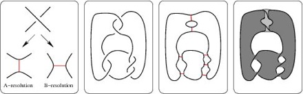
Figure 1. From left to right: $A$– and $B$–resolutions of a crossing, a link diagram, the ribbon graph ${\mathbb{G}_{A}}$ and the surface $S_{A}$. (Graphics by Jessica S. Purcell.)

Definition 2.1.

A spanning sub-graph ${\mathbb{H}}\subset{\mathbb{G}}$ of a ribbon graph is obtained by removing edges from ${\mathbb{G}}$.

With this setting we recall the following spanning sub-graph expansion of the Kauffman bracket proven by Dasbach, Futer, Kalfagianni, Lin and Stoltzfus [5].

Theorem 2.2.

[5] Let ${\mathbb{G}_{A}}$ be the ribbon graph obtained from the all $A$-resolution of a connected link diagram $D(L)$. Then the Kauffman bracket of $D$ is given by

$$\langle D\rangle =\sum_{\mathbb{H}\subset{\mathbb{G}_{A}}}A^{e({\mathbb{G}_{A}})-2e(\mathbb{H})}(-A^{2}-A^{-2})^{f(\mathbb{H})-1},\textflorin$$

where $\mathbb{H}\subset{\mathbb{G}_{A}}$ ranges over all spanning sub-graphs of ${\mathbb{G}_{A}}$.

2.1. Semi-adequate links and ribbon graphs

Lickorish and Thistlethwaite introduced the notion of $A$ and $B$-adequate links and studied the properties of their link polynomials [19, 18].

Definition 2.3.

A link diagram $D$ is called $A$–adequate if the ribbon graph ${\mathbb{G}_{A}}$ corresponding to the all–$A$ state contains no 1–edge loops. A link is called $A$-adequate if it admits an $A$-adequate link diagram.

Similarly, $D$ is called $B$–adequate if the all–$B$ graph ${\mathbb{G}_{B}}$ contains no 1–edge loops. A link is called $B$-adequate if it admits an $B$-adequate link diagram.

A link is called semi-adequate if it is $A$-adequate or $B$-adequate.

Definition 2.4.

For a connected link diagram $D$ and $n>1$ let $D^{n}$ denote the diagram obtained from $D$ by taking $n$ parallel copies of $D$. Here the convention is that $D=D^{1}$. See Figure 2 for an example. Define

$$M(D):=e({\mathbb{G}_{A}})+2v({\mathbb{G}_{A}})-2,\ \ {\rm and}\ \ m(D):=-e({\mathbb{G}_{B}})-2v({\mathbb{G}_{B}})+2.$$

Figure 2. A link diagram and its 2-parallel

With the notation of Definition 2.4, it is known that, for every diagram $D$, the highest degree (resp. the lowest degree ) of $\langle D\rangle$ is bounded above by $M(D)$ (resp. $m(D)$). Moreover, if $D$ is $A$-adequate (resp. $B$-adequate) then this bound is sharp. See, for example, [18].

For $l\geq 0$, let $a_{M-l}{(D^{n})}$ denote the $l+1$-th coefficient $\langle D^{n}\rangle$, starting from the maximum possible degree $M(D^{n})$. In this paper we are interested in the first two coefficients $a_{M}{(D^{n})}$ and $a_{M-1}{(D^{n})}$. For $A$-adequate links we have $a_{M}{(D^{n})}=\pm 1$, for all $n>0$. On the other hand, Manchon [20] shows that all integers can be realized as $a_{M}{(D)}$ for some link diagram. Thus for $a_{M}{(D)}\neq 0,1,-1$, Manchon’s construction gives non $A$-adequate diagrams for which the upper bound on the degree of the Kauffman bracket $\langle D\rangle$ is sharp. In contrast to this, we show the following lemma which implies that the degree upper bound of $\langle D^{n}\rangle$ is sharp, for some $n>1$, if and only if $D$ is $A$-adequate.

Lemma 2.5.

We have that $a_{M}{(D^{n})}\neq 0$, for some $n>1$, if and only if $D$ is $A$-adequate. Equivalently, the diagram $D$ is not $A$-adequate if and only if $a_{M}{(D^{n})}=0$, for all $n>1$.

Proof.

It is known that if $D$ is $A$-adequate then $a_{M}{(D^{n})}=\pm 1$; hence one direction of the lemma follows. We will show that if $D$ is not $A$-adequate then $a_{M}{(D^{n})}=0$, for all $n>1$. For $n>1$ let ${\mathbb{G}_{A}}^{n}$ denote the all-$A$ ribbon graph corresponding to $D^{n}$. By Theorem 2.2, the contribution of a spanning sub-graph $\mathbb{H}\subset{\mathbb{G}_{A}}^{n}$ to $\langle D^{n}\rangle$ is given by

(1) $$X_{{\mathbb{H}}}:=A^{e({\mathbb{G}_{A}}^{n})-2e(\mathbb{H})}(-A^{2}-A^{-2})^{f(\mathbb{H})-1}.$$

A typical monomial of $X_{{\mathbb{H}}}$ is of the form $A^{e({\mathbb{G}_{A}}^{n})-2e({\mathbb{H}})+2f({\mathbb{H}})-2-4s}$, for $0\leq s\leq f({\mathbb{H}})-1$. For a monomial to contribute to $a_{M}(D)$ we must have

$$e({\mathbb{G}_{A}}^{n})-2e({\mathbb{H}})+2f({\mathbb{H}})-2-4s=e({\mathbb{G}_{A}}^{n})+2v({\mathbb{G}_{A}}^{n})-2,$$

or equivalently $f({\mathbb{H}})=v({\mathbb{G}_{A}}^{n})+e({\mathbb{H}})+2s.$ Now we have

$$2g({\mathbb{H}}) = 2k({\mathbb{H}})-v({\mathbb{G}_{A}}^{n})+e({\mathbb{H}})-f({\mathbb{H}})$$

$$= 2k({\mathbb{H}})-2v({\mathbb{G}_{A}}^{n})-2s,$$

or $g({\mathbb{H}})=k({\mathbb{H}})-v({\mathbb{G}_{A}}^{n})-s\geq 0$. But since $v({\mathbb{G}_{A}}^{n})\geq k({\mathbb{H}})$ (every component must have a vertex) and $s\geq 0$ we conclude that for a monomial of $X_{{\mathbb{H}}}$ to contribute to $a_{M}(D)$ we must have $s=g({\mathbb{H}})=0$ and $v({\mathbb{G}_{A}}^{n})=k({\mathbb{H}})$. Since $f({\mathbb{H}})=v({\mathbb{G}_{A}}^{n})+e({\mathbb{H}})$, the contribution of ${\mathbb{H}}$ to $a_{M}(D)$ is

(2) $$(-1)^{f({\mathbb{H}})-1}=(-1)^{v({\mathbb{G}_{A}}^{n})+e({\mathbb{H}})-1}.$$

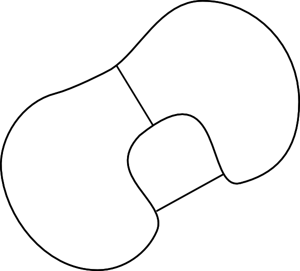
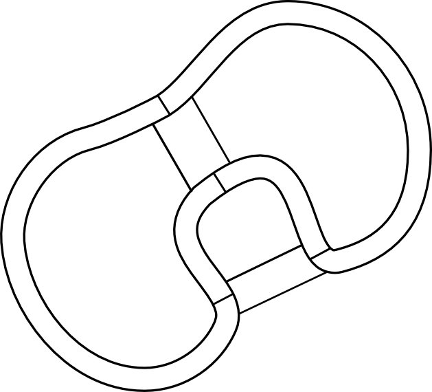
Figure 3. An example of ribbon graphs ${\mathbb{G}_{A}}$ and ${\mathbb{G}_{A}}^{2}$.

Since $D$ is not $A$-adequate, ${\mathbb{G}_{A}}$ must contain some loop edges. Thus $D^{n}$ also contains loop edges. Note that a sub-graphs of ${\mathbb{G}_{A}}$ all of whose edges are loops may have positive genus. Nevertheless for $n>1$ every sub-graph of ${\mathbb{G}_{A}}^{n}$ with only loop edges, must have genus zero as all the loop edges lie disjointly embedded on the same side of the vertex they are attached to. See Figure 3 for an example: The graph ${\mathbb{G}_{A}}$ in Figure 3 has genus one, since the two edges cannot be disjointly embedded on one side of the vertex. On the other hand in the graph ${\mathbb{G}_{A}}^{2}$ all the loop edges are embedded on one side of some loop; thus every subgraph with only loop edges has genus zero. Thus, if we let $\mathbb{L}_{n}\subset{\mathbb{G}_{A}}^{n}$ denote the maximal spanning sub-graph whose edges are all the loops of ${\mathbb{G}_{A}}^{n}$ then the sub-graphs of ${\mathbb{G}_{A}}^{n}$ that contribute to $a_{M}{(D^{n})}$ are in one to one correspondence with the sub-graphs of $\mathbb{L}_{n}$. Using equation 2, It follows that, for $n>1$,

(3) $$a_{M}{(D^{n})}=\sum_{\mathbb{H}\subset\mathbb{L}_{n}}(-1)^{e({\mathbb{H}})+v({\mathbb{G}_{A}}^{n})-1}=(-1)^{v({\mathbb{G}_{A}}^{n})-1}\left(\sum_{j=0}^{e(\mathbb{L}_{n})}{e(\mathbb{L}_{n})\choose j}(-1)^{j}\right)=0.$$

∎

Next we turn our attention to the second coefficient $a_{M-1}{(D^{n})}$. We have the following.

Lemma 2.6.

Suppose that $a_{M}{(D)}\neq 0$ and that $D$ is not $A$-adequate. Then we have $a_{M-1}{(D^{n})}=0$, for all $n>2$.

Proof.

For $n>2$ let ${\mathbb{G}_{A}}^{n}$ denote the all-$A$ ribbon graph corresponding to $D^{n}$.

As in [6], using Theorem 2.2, we see that a spanning sub-graph $\mathbb{H}\subset{\mathbb{G}_{A}}^{n}$ contributes to the term $a_{M-1}{(D^{n})}$ if and only if one of the following is true:

1. $v({\mathbb{H}})=k({\mathbb{H}})$ and $g({\mathbb{H}})=1$.

2. $v({\mathbb{H}})=k({\mathbb{H}})+1$ and $g({\mathbb{H}})=0$.

3. $v({\mathbb{H}})=k({\mathbb{H}})$ and $g({\mathbb{H}})=0$.

If $v({\mathbb{H}})=k({\mathbb{H}})$ then all the edges of ${\mathbb{H}}$ are loops. Since $n>2$, as in the proof of Lemma 2.5, subgraphs with only loop edges have genus 0. Thus we cannot have any ${\mathbb{H}}$ as in (1) above. Before we turn our attention to types (2) or (3) we need the following:

Claim. Let $\mathbb{H}\subset{\mathbb{G}_{A}}^{n}$ be a spanning subgraph that contains edges only on two vertices, say $v,v^{\prime}$, and such that $v({\mathbb{H}})=k({\mathbb{H}})+1$. Then, there is a spanning sub-graph $\mathbb{L}_{{\mathbb{H}}}\subset{\mathbb{G}_{A}}^{n}$ all of whose edges are loops and none of the edges is attached to the vertices $v,v^{\prime}$. See Figure 4 for an example of sub-graphs ${\mathbb{H}}$ and $\mathbb{L}_{{\mathbb{H}}}$.

Proof of Claim. Since $D$ is not $A$-adequate, ${\mathbb{G}_{A}}$ must contain some loop edges. Thus $D^{n}$ also contains loop edges. Since $a_{M}{(D)}\neq 0$, ${\mathbb{G}_{A}}$ contains a vertex, say $v_{1}$, that has loop edges attached to both sides; there are edges inside in $v_{1}$ and some loop edges outside of $v_{1}$, otherwise $a_{M}(D)$ would be equal to 0 (compare left picture of Figure 3). In ${\mathbb{G}_{A}}^{n}$, $v_{1}$ will correspond to $n$ state circles (resp. vertices) and two of those state circles will have loops on them: one set of loops, originally coming from inside of the state circle corresponding to $v_{1}$ in $D$, will be on the innermost state circle, while the loops coming from outside of $v_{1}$ will be on the outermost state circle (compare right picture of Figure 3). We will denote the two vertices corresponding to these state circles by $v_{I}$ and $v_{O}$, respectively. Since $n>2$, in ${\mathbb{G}_{A}}^{n}$ we have at least one vertex $v\neq v_{I},v_{O}$ that also comes from cabling $v_{1}$. Moreover, there are no edges of ${\mathbb{G}_{A}}^{n}$ with one end point on $v_{I}$ and the second on $v_{O}$.

Let $\mathbb{H}\subset{\mathbb{G}_{A}}^{n}$ be a spanning subgraph that contains edges only between two vertices, say $v,v^{\prime}$. By our discussion above, at least one of $v_{I}$ and $v_{O}$, say $v_{I}$, is different from $v,v^{\prime}$, and the claim follows.

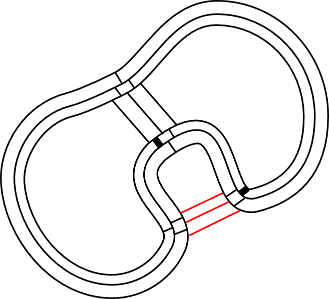
Figure 4. An example a ribbon graphs ${\mathbb{G}_{A}}^{3}$: The edges of a spanning sub-graph $H$ with $v({\mathbb{H}})=k({\mathbb{H}})+1$ are drawn thicker. The edges of the corresponding sub-graph $\mathbb{L}_{{\mathbb{H}}}$ are shown in red.

Now we show that the contribution of all sub-graphs satisfying (2) above to $a_{M-1}(D^{n})$ vanishes: The condition $v({\mathbb{H}})=k({\mathbb{H}})+1$ means that there are exactly two vertices in ${\mathbb{H}}$ with edges in ${\mathbb{H}}$ joining them. Consider the set $\mathcal{H}$ of sub-graphs of ${\mathbb{G}_{A}}^{n}$ with edges on exactly two vertices, where we must have edges joining these two vertices, and possibly loops on one of the vertices. Given ${\mathbb{H}}\in\mathcal{H}$, let $\mathbb{L}_{{\mathbb{H}}}\subset{\mathbb{G}_{A}}^{n}$ denote the maximal (i. e. the one with the most edges) sub-graph obtained from the claim above. That is, all the edges of $\mathbb{L}_{{\mathbb{H}}}$ are loops that are attached to vertices disjoint from the two vertices containing the edges of ${\mathbb{H}}$. Hence adding any subset of edges of $\mathbb{L}_{{\mathbb{H}}}$ to ${\mathbb{H}}$ also produces a subgraph of type (2) above. Moreover, all the sub-graphs of type (2) are obtained from an element of $\mathcal{H}$ in this fashion. The contribution of all type (2) subgraphs to $a_{M-1}{(D^{n})}$ is

$$\sum_{{\mathbb{H}}\in\mathcal{H}}\left(\sum_{j=0}^{e(\mathbb{L}_{{\mathbb{H}}})}{e(\mathbb{L}_{{\mathbb{H}}})\choose j}(-1)^{f({\mathbb{H}})+j}\right)=\sum_{{\mathbb{H}}\in\mathcal{H}}(-1)^{f({\mathbb{H}})}\left((1+(-1))^{e(\mathbb{L}_{{\mathbb{H}}})}\right)=0.$$

We now show that the contribution of type (3) sub-graphs to $a_{M-1}{(D^{n})}$ is also zero. As in the proof of Lemma 2.5, let $\mathbb{L}_{n}\subset{\mathbb{G}_{A}}^{n}$ denote the maximal spanning sub-graph whose edges are all the loops of ${\mathbb{G}_{A}}^{n}$. The subgraphs of type (3) are in one to one correspondence with the sub-graphs of $\mathbb{L}_{n}$. The contribution of these graphs is

(4) $$(-1)^{v({\mathbb{G}_{A}}^{n})-1}\sum_{\mathbb{H}\subset{\mathbb{G}_{A}}}e({\mathbb{H}})(-1)^{e({\mathbb{H}})},$$

where ${\mathbb{H}}$ ranges over all sub-graphs of ${\mathbb{G}_{A}}^{n}$. We have

$$\sum_{\mathbb{H}\subset{\mathbb{G}_{A}}}e({\mathbb{H}})(-1)^{e({\mathbb{H}})} = \sum_{j=0}^{e(\mathbb{L}_{n})}\left(e(\mathbb{L}_{n})-j\right){e(\mathbb{L}_{n})\choose j}(-1)^{e(\mathbb{L}_{n})-j}$$

$$= e(\mathbb{L}_{n})\sum_{j=0}^{e(\mathbb{L}_{n})}{e(\mathbb{L}_{n})\choose j}(-1)^{e(\mathbb{L}_{n})-j}-\sum_{j=1}^{e(\mathbb{L}_{n})}j{e(\mathbb{L}_{n})\choose j}(-1)^{e(\mathbb{L}_{n})-j}$$

$$= (-1)^{e(\mathbb{L}_{n})}\left(e(\mathbb{L}_{n})\sum_{j=0}^{e(\mathbb{L}_{n})}{e(\mathbb{L}_{n})\choose j}(-1)^{j}+\sum_{j=1}^{e(\mathbb{L}_{n})}j{e(\mathbb{L}_{n})\choose j}(-1)^{j-1}\right)$$

$$= (-1)^{e(\mathbb{L}_{n})}\left(e(\mathbb{L}_{n})f(-1)+f^{\prime}(-1)\right)=0,$$

where $f(x):=(1+x)^{{e(\mathbb{L}_{n})}}$ and $f^{\prime}(x)=e(\mathbb{L}_{n})(1+x)^{{e(\mathbb{L}_{n})-1}}$, the first derivative of $f(x)$. Thus the quantity in equation 4 is zero as desired.

∎

Remark 2.7.

The assumption $a_{M}{(D)}\neq 0$ in the statement of Lemma 2.6 is not necessary. However the proof given above does not go through without the restriction that $a_{M}{(D)}\neq 0$ . In the general case the proof will follow from the arguments in [16].

3. Colored Jones polynomial relations

A good reference for the following discussion is Lickorish’s book [18]. The colored Jones polynomials of a link $K$ have a convenient expression in terms of Chebyshev polynomials. For $n\geq 0$, the polynomial $S_{n}(x)$ is defined recursively as follows:

(5) $$S_{n+1}(x)=xS_{n}(x)-S_{n-1}(x),\qquad S_{1}(x)=x,\qquad S_{0}(x)=1.$$

Let $D$ be a diagram of a link $K$. Recall that for an integer $m>0$, $D^{m}$ denotes the diagram obtained from $D$ by taking $m$ parallel copies of $K$. This is the $m$–cable of $D$ using the blackboard framing; if $m=1$ then $D^{1}=D$. Recall that $\langle D^{m}\rangle$ denotes the Kauffman bracket of $D^{m}$. Let $c_{+}=c_{+}(D)$ and $c_{-}=c_{-}(D)$ denote the number of positive and negative crossings of $D$ and let $w=w(D)=c_{+}-c_{-}$ denote the writhe of $D$. Then we may define the function

(6) $$G_{D}(n+1,A):=\left((-1)^{n}A^{n^{2}+2n}\right)^{-w}(-1)^{n-1}\langle S_{n}(D)\rangle,$$

where $S_{n}(D)$ is a linear combination of blackboard cabling of $D$, obtained via equation (5) and the bracket is extended linearly. For the results below, the important corollary of the recursive formula for $S_{n}(x)$ is that

(7) $$S_{n}(D)=D^{n}+(1-n)D^{n-2}+\mbox{lower degree cablings of }D.$$

The reduced $(n+1)$–colored Jones polynomial of $K$, denoted by $J_{K}(n+1,q)$, is obtained from $\left(\frac{A^{4}-A^{-4}}{A^{2n}-A^{-2n}}\right)G(n+1,A)$ by substituting $q:=A^{-4}$. The ordinary Jones polynomial corresponds to $n=1$.

3.1. Bounds on the degree of colored Jones polynomials

Given a link diagram $D(L)$, let $v_{A}(D)$ denote the number of components resulting from $D$ by applying the all-$A$ Kauffman state. For $n\in{\mathbb{N}}$ let

$$h_{n}(D):=2{c_{-}(D)}n^{2}+2\left(v_{A}(D)-w(D)\right)n-2.$$

Let $d(n)$ denote the maximum degree in $A$ of $G_{D}(n+1,A)$ . It is know that, for every $n>0$, $d(n)\leq h_{n}(D)$ and that if $D$ is a $A$-adequate diagram then

(8) $$d(n)=h_{n}(D)=2{c_{-}(D)}n^{2}+2\left(v_{A}(D)-w(D)\right)n-2,$$

and the coefficient of this leading terms is known to be $\pm 1$. For $n=1$ the equation 8 is not enough to characterize $A$-adequate diagrams: Manchon [20] shows that all non-zero integers can be realized as leading coefficients of Jones polynomials of knots with diagrams satisfying equation 8. Links realizing integers $a_{M}\neq-1,1$ will necessarily be non $A$-adequate. It follows that there exist infinitely many links $L$ that admit diagrams $D$ with $d(1)=h_{1}(D)$ but $D$ or $L$ is non-adequate. In contrast to this, in this paper we have:

Theorem 3.1.

Let $D$ be a diagram of a link $K$ and let $h_{n}(D)$, $d(n)$ and $G_{D}(n+1,A)$ be as above. Then, $D$ is $A$-adequate if and only if we have $d(n)=h_{n}(D)$, for some $n\geq 2$.

Furthermore, we have $d(n)=h_{n}(D)$, for every $n\geq 2$, if and only if $d(2)=h_{2}(D)$.

Proof.

By equations 6 and 7 the coefficient of $A^{h_{n}(D)}$ in $G_{D}(n+1,A)$ is the same, in absolute value, as $a_{M(D^{n})}$. Thus, the theorem follows immediately by Lemma 2.5. ∎

Remark 3.2.

Theorem 3.1 should be compared with the main results of [22] where Thistlethwaite shows that part of the 2-variable Kauffman polynomial where the total degree is the number of crossings in a link diagram, is non-zero if and only if the diagram is $A$-adequate.

3.2. Stable invariants

On the set of oriented link diagrams consider the complexity

$$\left(c_{-}(D),\ c(D),\ v_{A}(D)-w(D)\right),$$

ordered lexicographically. For a link $K$ define ${\mathcal{D}}(K)$ to be the set of diagrams representing $K$ and minimize this complexity. More specifically, we define ${\mathcal{D}}(K)$ as follows: First consider the set of all diagrams of $K$ that minimize the number of negative crossings $c_{-}$; call this minimum number $c_{-}(K)$. Then, within this set restrict to the subset say $X_{K}$ of diagrams that have minimum crossing number: that is $D\in X_{K}$ if and only if $c(D)\leq c(D^{\prime})$, for all diagrams of $K$ with $c_{-}(D)=c_{-}(K)$. Since there are only finitely many diagrams of bounded crossing number, given a link $K$, the set $X_{K}$ is finite. Thus we may define

$${\mathcal{D}}(K):=\{D\in X_{K}\ |\ v_{A}(D)-w(D)\leq v_{A}(D^{\prime})-w(D^{\prime}),{\rm for}\ {all}\ D^{\prime}\in X_{K}\}.$$

Lemma 3.3.

Suppose that for a link $K$, there is $D\in{\mathcal{D}}(K)$ that is $A$-adequate. Then, all the diagrams in ${\mathcal{D}}(K)$ are $A$-adequate.

Proof.

Suppose that $D\in{\mathcal{D}}(K)$ is $A$-adequate and let $D^{\prime}$ be another diagram in $D\in{\mathcal{D}}(K)$. Since $D,D^{\prime}\in{\mathcal{D}}(K)$, we have $c_{-}(D)=c_{-}(D^{\prime})$ and $v_{A}(D)-w(D)=v_{A}(D^{\prime})-w(D^{\prime})$. Thus $h_{n}(D)=h_{n}(D^{\prime})$. Since $D$ is $A$-adequate, we have $d(n)=h_{n}(D)=h_{n}(D^{\prime})$, for all $n>0$. Thus, by Theorem 3.1, $D^{\prime}$ is $A$-adequate. ∎

Definition 3.4.

Given a link $K$ and a link diagram $D\in{\mathcal{D}}(K)$ we define $T_{(D,n)}(q)$ as follows: For $n>2$, define

(9) $$\alpha(D,n):={\left|a_{M}{(D)}a_{M}{(D^{n})}\right|}\ \ \ \ {\rm and}\ \ \ \ \beta(D,n):={\left|a_{M}{(D)}a_{M-1}(D^{n})\right|}.$$

Now let $T_{(D,n)}(q):=\alpha(D,n)+\beta(D,n)q$.

Now we will show that the quantities defined in equation 9 are in fact independent of $n$ and of the diagram $D$.

Corollary 3.5.

The quantities, $\alpha(D,n)$ and $\beta(D,n)$ defined above are independent of the diagram $D\in{\mathcal{D}}(K)$ and of $n$. Thus they are invariants of $K$ denoted by $\alpha_{K}$ and $\beta_{K}$.

Proof.

Suppose that $K$ is not $A$-adequate and let $D\in{\mathcal{D}}(K)$. Then by Theorem 3.1 we have $a_{M}{(D^{n})}=0$ for every $n>1$ and every $D\in{\mathcal{D}}(K)$. Thus by equation 9 we have $\alpha(D,n)=0$. If $a_{M}(D)=0$, then equation 9 implies $\beta(D,n)=0$. Suppose $a_{M}(D)\neq 0$. Then by Lemma 3.3, $a_{M-1}{(D^{n})}=0$, thus $\beta(D,n)=0$. Thus, in this case, the definition $\alpha(D,n)=\beta(D,n)=0$, for every $n>1$ and $D\in{\mathcal{D}}(K)$.

Suppose now that $K$ is $A$-adequate. By Lemma 3.3, for every $D\in{\mathcal{D}}(K)$, $D$ is an $A$-adequate diagram. Then, by [18] we have $\alpha(D,n)=1$, for all $n>0$. Similarly $\beta(D,n)$ is the absolute value of the penultimate coefficient of $J_{K}(n+1,q)$ and thus an invariant of $K$. By [7], $\beta(D,n)$ is also independent of $n$. ∎

Define the linear polynomial in $q$, $T_{K}(q):=\alpha_{K}+\beta_{K}q$. This is an invariant of $K$ that detects exactly when $K$ is $A$-adequate. More specifically we have the following:

Corollary 3.6.

We have $T_{K}(q)\neq 0$ if and only $K$ is $A$-adequate. Furthermore, if $T_{K}(q)=1$, then $K$ is fibered.

Proof.

As already mentioned in the proof of Corollary 3.5, if $K$ is not $A$-adequate, then $T_{K}(q)=0$. On the other hand, if $K$ is $A$-adequate then we know that $\alpha_{K}=1$ and thus $T_{K}(q)\neq 0$.

Suppose now that $T_{K}(q)=1$. Then, in particular, $\beta_{K}=0$. By Corollary 9.16, of [10], $K$ has to be fibered. ∎

3.3. Stabilization properties of Jones polynomials

The coefficients of the colored Jones polynomials of $A$-adequate links have stabilization properties that have been studied by several authors in the recent years [7, 1, 13]. Dasbach and Lin observed that the last three coefficients of $J_{K}(n+1,q)$ stabilize. Armond [1] and Garoufalidis and Le [13] generalized this phenomenon to show the following: For every $i>0$ the $i$-th to last coefficient of $J_{K}(n+1,q)$, stabilizes for $i\geq n$. These coefficients can be put together to form the tail of the colored Jones polynomial. In the case of $A$-adequate links the invariants $\beta_{K},\alpha_{K}$ defined above, are the last couple of stable coefficients. In fact, Garoufalidis and Le have studied the “higher order” stability properties of the colored Jones polynomials and they showed that the stable coefficients of the polynomials $J_{K}(n+1,q)$ give rise to infinitely many $q$-series with interesting number theoretic and physics connections. On the other hand, the work of Futer, Kalfagianni and Purcell [8, 9, 10, 12, 11] showed that certain stable coefficients of $J_{K}(n+1,q)$ encode information about incompressible surfaces in knot complements and their geometric types and have direct connections to hyperbolic geometry. See also discussion below. Rozansky [17] showed that the stability behavior also appears in the categorifications of the colored Jones polynomials [17].

The structure of the colored Jones polynomials of non-semi-adequate links and its geometric content are much less understood. In a forthcoming paper [16], C. Lee generalizes Theorem 3.1 to show the following: If $D$ is not $A$-adequate, then, we have $d(n)\leq h_{n}(D)-(n-1)$, for every $n\geq 2$. This implies that the first $n-1$ coefficients of $G_{D}(n+1,A)$, starting from the one for degree $h_{n}(D)$, are zero, for every $n\geq 2$. Given a link $K$ and a link diagram $D\in{\mathcal{D}}(K)$ one can define a power series $J^{0}=J^{0}(D)$ as follows: Define $\beta_{1}=\beta_{1}(D)$ to be the coefficient of $A^{h_{2}(D)}$ in $G_{D}(3,A)$. For $i>1$, define $\beta_{i}=\beta_{i}(D)$ to be the coefficient of $A^{h_{i+1}(D)-4(i-1)}$. Now let

$$J^{0}_{K}(q)=\sum_{i=1}^{\infty}\beta_{i}q^{i-1}.$$

Lee shows that $J^{0}_{K}(q)\neq 0$, if and only if $K$ is $A$-adequate. This shows that the coefficients of $J_{K}(n+1,q)$, at the level where the tail of semi-adequate links occurs, also stabilize but the corresponding tail is trivial. This was conjectured by Rozansky in [17] where he also conjectures that this behavior should persist in the setting of categorification (Conjecture 2.13 of [17]).

3.4. Detecting incompressible surfaces and their geometric types

For every $D\in{\mathcal{D}}(K)$ we obtain a surface $S_{A}$, as follows. Each state circle of $v_{A}(D)$ bounds a disk in $S^{3}$. This collection of disks can be disjointly embedded in the ball below the projection plane. At each crossing of $D$, we connect the pair of neighboring disks by a half-twisted band to construct a surface $S_{A}\subset S^{3}$ whose boundary is $K$. See Figure 1 for an example. By the work of the first author with Futer and Purcell [10, 12], the invariant $T_{K}(q)$ detects the geometric types of the surface $S_{A}(D)$ and contains a lot of information about the geometric structures of of the complements $S^{3}{\backslash\backslash}S_{A}(D)$ and $S^{3}{\smallsetminus}K$. For example, combining Corollary 3.6 with results of [10, 12] we have the following; for terminology and more details the reader is referred to the original references.

Corollary 3.7.

The invariant $T_{K}(q)$ has the following properties:

1. For every $D\in{\mathcal{D}}(K)$, the surface $S_{A}(D)$ is essential (i.e. $\pi_{1}$-injective) in $S^{3}{\smallsetminus}K$ if and only if $T_{K}(q)\neq 0$.

2. For every $D\in{\mathcal{D}}(K)$, the surface $S_{A}(D)$ is a fiber in the complement $S^{\smallsetminus}K$ if and only if $T_{K}(q)=1$.

3. Suppose that $K$ is hyperbolic. Then, for every $D\in{\mathcal{D}}(K)$, the surface $S_{A}(D)$ is quasifuschian $S^{3}{\smallsetminus}K$ if and only if $T_{K}(q)\neq 0,1$.

Proof.

By Theorem 3.19 of [10] $S_{A}(D)$ is essential precisely when $D$ is $A$-adequate. Thus part (1) follows from Corollary 3.6. For part (2), first note that if $T_{K}(q)=1$ then, by Theorem 3.1, $K$ is $A$-adequate. Thus, $\beta_{K}$ is, in absolute value, the penultimate stable coefficient of the colored Jones polynomial in the sense of [7]. Now by [10], $\beta_{K}=0$ if and only if $S_{A}(D)$ is a fiber in the complement $S^{\smallsetminus}K$ . Finally for (3) we note that $T_{K}(q)\neq 0$, then again by Theorem 3.1, if and only if $K$ is $A$-adequate. Now $T_{K}(q)\neq 1$, if and only $\beta_{K}\neq 0$. Then, by Theorem 1.4 of [12] $\beta_{K}\neq 0$ if and only if the surface $S_{A}(D)$ is quasifuchsian for every $A$-adequate diagram $D$. ∎

Acknowledgement. This work started while the authors were attending the conference Quantum Topology and Hyperbolic Geometry in Nha Trang, Vietnam (May 13-17, 2013). We thank the organizers, Anna Beliakova, Stavros Garoufalidis, Phung Hai, Vu Khoi, Thang Le, Chu Loc, and Phan Phien for their hospitality and for providing excellent working conditions. We also thank Lev Rozansky for a useful conversation during the same conference.

References

- [1] Cody Armond, The head and tail conjecture for alternating knots., arXiv:1112.3995.
- [2] Cody Armond and Oliver T. Dasbach, The head and tail of the colored jones polynomial for adequate knots, arXiv:1310.4537.
- [3] by same author, Rogers–Ramanujan type identities and the head and tail of the colored Jones polynomial, arXiv:1106.3948.
- [4] Béla Bollobás and Oliver Riordan, A polynomial invariant of graphs on orientable surfaces, Proc. London Math. Soc. (3) 83 (2001), no. 3, 513–531.
- [5] Oliver T. Dasbach, David Futer, Efstratia Kalfagianni, Xiao-Song Lin, and Neal W. Stoltzfus, The Jones polynomial and graphs on surfaces, Journal of Combinatorial Theory Ser. B 98 (2008), no. 2, 384–399.
- [6] by same author, Alternating sum formulae for the determinant and other link invariants, J. Knot Theory Ramifications 19 (2010), no. 6, 765–782.
- [7] Oliver T. Dasbach and Xiao-Song Lin, On the head and the tail of the colored Jones polynomial, Compositio Math. 142 (2006), no. 5, 1332–1342.
- [8] David Futer, Efstratia Kalfagianni, and Jessica S. Purcell, Dehn filling, volume, and the Jones polynomial, J. Differential Geom. 78 (2008), no. 3, 429–464.
- [9] by same author, Slopes and colored Jones polynomials of adequate knots, Proc. Amer. Math. Soc. 139 (2011), 1889–1896.
- [10] by same author, Guts of surfaces and the colored Jones polynomial, Lecture Notes in Mathematics, vol. 2069, Springer, Heidelberg, 2013.
- [11] by same author, Jones polynomials, volume, and essential knot surfaces: a survey, Proceedings of Knots in Poland III, Banach Center Publications (to appear), arXiv:1110.6388.
- [12] by same author, Quasifuchsian state surfaces, Trans. Amer. Math. Soc. (to appear), arXiv:1209.5719.
- [13] Stavros Garoufalidis and Thang T. Q. Lê, Nahm sums, stability and the colored jones polynomial, arXiv:1112.3905.
- [14] Stavros Garoufalidis, Sergei Norin, and Thao Vong, Flag algebras and the stable coefficients of the jones polynomial, arXiv:1309.5867.
- [15] Stavros Garoufalidis and Thao Vong, A stability conjecture for the colored jones polynomial.
- [16] Christine Ruey Shan Lee, Stabillity properties of the colored jones polynomial, in preparation.
- [17] Rozansky Lev, Khovanov homology of a unicolored b-adequate link has a tail., arXiv:1203.5741.
- [18] W. B. Raymond Lickorish, An introduction to knot theory, Graduate Texts in Mathematics, vol. 175, Springer-Verlag, New York, 1997.
- [19] W. B. Raymond Lickorish and Morwen B. Thistlethwaite, Some links with nontrivial polynomials and their crossing-numbers, Comment. Math. Helv. 63 (1988), no. 4, 527–539.
- [20] P. M. G. Manchón, Extreme coefficients of Jones polynomials and graph theory, J. Knot Theory Ramifications 13 (2004), no. 2, 277–295.
- [21] Alexander Stoimenow, Coefficients and non-triviality of the jones polynomial, J. Reine Angew. Math. (2011), DOI: 10.1515/CRELLE.2011.047.
- [22] Morwen B. Thistlethwaite, On the Kauffman polynomial of an adequate link, Invent. Math. 93 (1988), no. 2, 285–296.