PACS: 42.50.-p, 03.67.-a, 03.65.Sq, 03.67.Dd

Acknowledgements The authors would like to thank Prof. E. Santos for revising the manuscript, and for helpful suggestions and comments on the work. A. Casado acknowledges the support from the Spanish MCI Project no. FIS2011-29400.

Abstract

We apply the Wigner formalism of quantum optics in the Heisenberg picture to study the role of the zeropoint field fluctuations in entanglement swapping produced via parametric down conversion. It is shown that the generation of mode entanglement between two initially non interacting photons is related to the quadruple correlation properties of the electromagnetic field, through the stochastic properties of the vacuum. The relationship between the process of transferring entanglement and the different zeropoint inputs at the nonlinear crystal and the Bell-state analyser is emphasized.

Keywords: Entanglement swapping, Bell-state analysis, teleportation, parametric down conversion, Wigner representation, zeropoint field.

1 Introduction

The theory of quantum information in quantum optics is supported by the phenomena of entanglement [1, 2] and hyperentanglement [3, 4, 5] produced via parametric down conversion (PDC) [6, 7, 8, 9]. These phenomena constitute a very important experimental arena for quantum cryptography [10, 11], dense coding [12], superdense coding [13] and teleportation [14, 15, 16, 17]. The ultimate goal would be to build a quantum computer network for the transmission and reconstruction over an arbitrary distance of a quantum state, but for the latter, it would be necessary to build a network of repeaters [18, 19, 20, 21, 22, 23] whose physical base is the process known as entanglement swapping [24]. This implies that two particles which have never interacted are entangled as a consequence of a Bell state measurement (BSM) [25, 26], involving two Einstein-Podolsky-Rosen (EPR) pairs [1]. In 2000, Asher Peres [27] put forward the paradoxical idea that entanglement could be produced after the entangled particles have been measured, even if they no longer exist. This can also be viewed as quantum steering into the past. Recent studies appear to confirm this paradox [28]. More recently, it has been demonstrated that entanglement can be transferred to two photons that exist at separate times [29].

The Wigner formalism constitutes a complementary approach to the standard Hilbert-space formulation for the study of optical quantum information processing and for its practical implementation using PDC. In the Wigner representation within the Heisenberg picture (WRHP), the Wigner function is time independent, it corresponds to the Wigner distribution of the initial state of the electromagnetic field, and the dynamics is contained in the electric field amplitudes. The analysis of the generation and propagation of PDC light with this formalism was treated in a series of papers using a Hamiltonian approach [30, 31] and also by starting from the Maxwell equations inside the crystal [32]. The WRHP approach resembles classical optics, in the sense that the light emitted by the crystal is generated via the coupling between the zeropoint field (ZPF) and the laser beam entering the nonlinear medium, which gives rise to an amplification of vacuum fluctuations. The Wigner function is positive in this case, it corresponds to the Gaussian Wigner distribution of the vacuum amplitudes. Finally, the zeropoint fluctuations are subtracted at the detectors, and the theory of detection in the Wigner approach shows how the signal is separated from the ZPF background. These two features, zeropoint field and its subtraction in the detection process, constitute the main differences with respect to classical optics, and give rise to the typical results within the quantum domain.

The WRHP formalism has been applied recently to the study of experiments on quantum communication using PDC. For instance, quantum cryptography with entangled photons [33], partial Bell-state measurement [34], and polarization-momentum hyperentanglement and its application to complete Bell-state measurement [35]. The essential point of the WRHP formalism is that it focuses on the relationship between the correlation properties of the light field in a concrete experiment, through the propagation of the zeropoint field amplitudes, and the corresponding optical quantum communication protocol. As a matter of fact, a key point of this approach is that entanglement can be seen just as an interplay of correlated waves, which sharply contrasts to the usual Hilbert-space or more particle-based formalism [30]. Also there is a double role of the zeropoint field in this kind of experiments: it carries the quantum information that is extracted at the source and introduces a fundamental noise at the idle channels of the analysers, which limits the information that can be efectively measured [35]. Hence, the WRHP formalism offers a complementary wave-like reinterpretation of experiments on quantum communication involving PDC light, to the one provided by the standard Hilbert-space description based on the concept of qubit, in which the corpuscular aspect of light is emphasized.

In this paper we shall analyze the relationship between entanglement swapping using PDC and the zeropoint field fluctuations by using the WRHP formalism. As we shall show throughout this document, the fundamental concept for understanding the phenomenon of teleportation of entanglement, is the quadruple correlation of the electromagnetic field. Our analysis using the WRHP approach will contrast, apparently, to the usual explanation in terms of the collapse of the state vector at the Bell-state analyser. The link between both formalisms is found to be in the zeropoint field amplitudes, but the importance of this work goes beyond the mathematical aspects, giving rise to new results.

This paper is organised as follows: In Section 2 we shall give the WRHP description of the basic quantum state for entanglement swapping [36], and we shall calculate the field amplitudes at the detectors. We shall show that, in order to generate the two pair of entangled beams, eight sets of independent zeropoint modes (four sets for each emission) are necessary. In Subsection 2.1 we shall calculate the cross-correlation properties of the light field. In Section 3 the quadruple correlations leading to four fold-coincidence will be analysed, and the intrinsic nature of teleportation based in the zeropoint field amplitudes will be revealed. Finally, in Section 4 we shall discuss the main results of this work, and we shall present the conclussions and further steps of this research line. In Appendix A we present a brief summary of the most important concepts and results of the WRHP formalism of PDC, which are used in this paper. In addition, we have included in Appendix B the calculation of the quadruple detection probability in the WRHP approach.

2 Entanglement Swapping in the WRHP formalism

Entanglement swapping [24, 37, 38, 39, 40] provides a method of entanglement of two particles that do not interact. Let us review the basic aspects of this process in the Hilbert space [41]. Two EPR sources generate, independently, two pairs of entangled particles, pair $1$-$2$ and pair $3$-$4$, being each pair described by a singlet state. Particles $2$ and $3$ are subjected to a Bell state analysis as shown in Figure 1. The collapse of the state vector to a given eigenstate of particles $2$ and $3$ gives rise to an entanglement between particles $1$ and $4$, which is called entanglement teleportation or entanglement swapping.

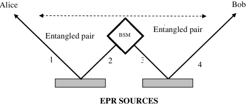
Figure 1: Principle of entanglement swapping.

The total state describes the fact that particles $1$ and $2$ ($3$ and $4$) are entangled in a singlet state. For instante, if we are dealing with polarization entanglement, we have:

$$|\Pi\rangle_{1234}=|\Psi^{-}\rangle_{12}|\Psi^{-}\rangle_{34}$$

$$=\frac{1}{2}(|\Psi^{+}\rangle_{14}|\Psi^{+}\rangle_{23}-|\Psi^{-}\rangle_{14}|\Psi^{-}\rangle_{23}-|\Phi^{+}\rangle_{14}|\Phi^{+}\rangle_{23}+|\Phi^{-}\rangle_{14}|\Phi^{-}\rangle_{23}),$$ (1)

where

$$|\Psi^{\pm}\rangle_{ij}=\frac{1}{\sqrt{2}}(|H\rangle_{i}|V\rangle_{j}\pm|V\rangle_{i}|H\rangle_{j})\,\,\,;\,\,\,|\Phi^{\pm}\rangle_{ij}=\frac{1}{\sqrt{2}}(|H\rangle_{i}|H\rangle_{j}\pm|V\rangle_{i}|V\rangle_{j}),$$ (2)

are the polarization Bell base states. Factoring is a consequence of the pairs being independent. Nevertheless, a BSM on particles $2$ and $3$ will leave particles $1$ and $4$ entangled in the same state as the corresponding to the projective measurement on the pair $2-3$. In this way, particles $1$ and $4$ will end up in one of the four Bell states: $|\Psi_{14}^{+}\rangle$, $|\Psi_{14}^{-}\rangle$, $|\Phi_{14}^{+}\rangle$ and $|\Phi_{14}^{-}\rangle$, with the same $1/4$ probability. In the case of light, it is well known that the four Bell states are not distinguishable when entanglement in only one degree of freedom is considered [42]. In the last decade, the problem of performing complete Bell-state measurement with photons has been solved using hyperentanglement [5].

The quantum predictions corresponding to the state $|\Pi\rangle_{1234}=|\Psi^{-}\rangle_{12}|\Psi^{-}\rangle_{34}$ are reproduced in the WRHP approach (see Appendix A) via the consideration of the following four beams (see Fig. 2), which are generated from the coupling inside the nonlinear medium between the laser field and the ZPF inputs (see Eqs. (A.13) and (A.14)):

$$\begin{array}[]{l}{\bf{F}}_{1}^{(+)}({\bf r}_{S_{1}},t)={F^{\prime}}_{s}^{(+)}({\bf r}_{S_{1}},t;\{\alpha_{{\bf{k}}_{1},H};\alpha^{*}_{{\bf{k}}_{2},V}\}){\bf{i}}_{1}+{F^{\prime}}_{p}^{(+)}({\bf r}_{S_{1}},t;\{\alpha_{{\bf{k}}_{1},V};\alpha^{*}_{{\bf{k}}_{2},H}\}){\bf{j}}_{1},\end{array}$$ (3)

$$\begin{array}[]{l}{\bf{F}}_{2}^{(+)}({\bf r}_{S_{1}},t)={F^{\prime}}_{q}^{(+)}({\bf r}_{S_{1}},t;\{\alpha_{{\bf{k}}_{2},H};\alpha^{*}_{{\bf{k}}_{1},V}\}){\bf{i}}_{2}-{F^{\prime}}_{r}^{(+)}({\bf r}_{S_{1}},t;\{\alpha_{{\bf{k}}_{2},V};\alpha^{*}_{{\bf{k}}_{1},H}\}){\bf{j}}_{2},\end{array}$$ (4)

$$\begin{array}[]{l}{\bf{F}}_{3}^{(+)}({\bf r}_{S_{2}},t)=F_{s}^{(+)}({\bf r}_{S_{2}},t;\{\alpha_{{\bf{k}}_{3},H};\alpha^{*}_{{\bf{k}}_{4},V}\}){\bf{i}}_{3}+F_{p}^{(+)}({\bf r}_{S_{2}},t;\{\alpha_{{\bf{k}}_{3},V};\alpha^{*}_{{\bf{k}}_{4},H}\}){\bf{j}}_{3},\end{array}$$ (5)

$$\begin{array}[]{l}{\bf{F}}_{4}^{(+)}({\bf r}_{S_{2}},t)=F_{q}^{(+)}({\bf r}_{S_{2}},t;\{\alpha_{{\bf{k}}_{4},H};\alpha^{*}_{{\bf{k}}_{3},V}\}){\bf{i}}_{4}-F_{r}^{(+)}({\bf r}_{S_{2}},t;\{\alpha_{{\bf{k}}_{4},V};\alpha^{*}_{{\bf{k}}_{3},V}\}){\bf{j}}_{4},\end{array}$$ (6)

where we have considered that the center of the first (second) nonlinear source is located at position ${\bf r}_{S_{1}}$ (${\bf r}_{S_{2}}$). We have included the sets of zeropoint modes that appear in each electric field component [34]. The only non-null cross-correlations are those concerning the labels $(p,q)$ and $(r,s)$ of beams $1-2$, and the same for the beams $3-4$, i.e. the non-null cross-correlations correspond to different polarization components, and there is a sign difference between the two correlations involving the couple of beams $1-2$ ($3-4$), as it can be seen from Eqs. (3) and (4) [(5) and (6)]. On the other hand, there is no cross-correlation involving any of the primed amplitudes (beams $1-2$) with the unprimed ones (beams $3-4$).

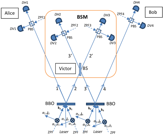
Figure 2: Entanglement swapping via two nonlinear crystals. Each couple of down converted photons is generated through the coupling inside the nonlinear source between the laser and four sets of independent zeropoint modes. This is an essential aspect in the WRHP description for PDC experiments.

Taking into account the propagation of the field amplitudes [see Eq. (A.3)] we can express all the cross-correlations, at any position and time, in terms of the corresponding ones at the center of the nonlinear sources [31]. For instance (see Eq. (A.15)):

$$\langle F^{(+)}_{p}({\bf r}_{S_{2}},t)F^{(+)}_{q}({\bf r}_{S_{2}},t^{\prime})\rangle=gV\nu(t^{\prime}-t).$$ (7)

A similar expression holds for $\langle F^{(+)}_{r}({\bf r}_{S_{2}},t)F^{(+)}_{s}({\bf r}_{S_{2}},t^{\prime})\rangle$, and also for the corresponding primed amplitudes, which are emitted at the first crystal.

Let us emphasize that beams $1$ and $2$ are completely uncorrelated with beams $3$ and $4$, given that the vacuum modes that are involved in the couple $1-2$ share no correlation with the corresponding vacuum modes in the couple $3-4$, as it can be easily seen from Eq. (A.5). This is closely related to the factorization in Eq. (1).

Where is the origin of entanglement swapping in the WRHP formalism? The answer to this question is centralised in how the correlations change, after beams $2$ and $3$ cross the balanced beam-splitter (BS). The action of the BS on beams $2$ and $3$ produces beams ${\bf{F}}_{3^{\prime}}^{(+)}$ and ${\bf{F}}_{2^{\prime}}^{(+)}$:

$${\bf{F}}_{3^{\prime}}^{(+)}({\bf r}_{BS},t)=\frac{1}{\sqrt{2}}[i{F^{\prime}}_{q}^{(+)}({\bf r}_{BS},t)+F_{p}^{(+)}({\bf r}_{BS},t)]{\bf{i}}_{3^{\prime}}$$

$$+\frac{1}{\sqrt{2}}[i{F^{\prime}}_{r}^{(+)}({\bf r}_{BS},t)+F_{s}^{(+)}({\bf r}_{BS},t)]{\bf{j}}_{3^{\prime}},$$ (8)

$${\bf{F}}_{2^{\prime}}^{(+)}({\bf r}_{BS},t)=\frac{1}{\sqrt{2}}[{F^{\prime}}_{q}^{(+)}({\bf r}_{BS},t)+iF_{p}^{(+)}({\bf r}_{BS},t)]{\bf{i}}_{2^{\prime}}$$

$$+\frac{1}{\sqrt{2}}[{F^{\prime}}_{r}^{(+)}({\bf r}_{BS},t)+iF_{s}^{(+)}({\bf r}_{BS},t)]{\bf{j^{\prime}}}_{2^{\prime}},$$ (9)

with ${\bf r}_{BS}$ being the position of the beam-splitter where the two beams are recombined. Now, we shall consider that the polarization beam splitters (PBS) transmit (reflect) horizontal (vertical) polarization. The electric field amplitude at the detectors will include the superposition of a zeropoint field component coming from the idle channels of the PBSs. We shall use unprimed (primed) space-time variables for characterizing the field amplitude at the detector corresponding to horizontal (vertical) polarization:

$$({\bf r}_{DHi},t_{DHi})\equiv({\bf r}_{i},t_{i})\,\,\,\,;\,\,\,\,({\bf r}_{DVi},t_{DVi})\equiv({\bf r^{\prime}}_{i},t^{\prime}_{i})\,\,\,\,;\,\,\,\,i=1,2,3,4.$$ (10)

In this way, the field amplitudes at the Bell-state analyser are:

$$\begin{array}[]{l}{\bf{F}}_{DH2}^{(+)}({\bf{r}}_{2},t_{2})=\frac{1}{\sqrt{2}}[i{F^{\prime}}_{q}^{(+)}({\bf{r}}_{2},t_{2})+F_{s}^{(+)}({\bf{r}}_{2},t_{2})]{\bf{i}}+i[{\bf{F}}_{ZPF2}^{(+)}({\bf{r}}_{2},t_{2})\cdot{\bf{j}}]{\bf{j}},\end{array}$$ (11)

$$\begin{array}[]{l}{\bf{F}}_{DV2}^{(+)}({\bf{r^{\prime}}}_{2},t^{\prime}_{2})=\frac{i}{\sqrt{2}}[i{F^{\prime}}_{r}^{(+)}({\bf{r^{\prime}}}_{2},t^{\prime}_{2})-F_{p}^{(+)}({\bf{r^{\prime}}}_{2},t^{\prime}_{2})]{\bf{j}}+[{\bf{F}}_{ZPF2}^{(+)}({\bf{r^{\prime}}}_{2},t^{\prime}_{2})\cdot{\bf{i}}]{\bf{i}},\end{array}$$ (12)

$$\begin{array}[]{l}{\bf{F}}_{DH3}^{(+)}({\bf{r}}_{3},t_{3})=\frac{1}{\sqrt{2}}[{F^{\prime}}_{q}^{(+)}({\bf{r}}_{3},t_{3})+iF_{s}^{(+)}({\bf{r}}_{3},t_{3})]{\bf{i^{\prime}}}+i[{\bf{F}}_{ZPF3}^{(+)}({\bf{r}}_{3},t_{3})\cdot{\bf{j^{\prime}}}]{\bf{j^{\prime}}},\end{array}$$ (13)

$$\begin{array}[]{l}{\bf{F}}_{DV3}^{(+)}({\bf{r^{\prime}}}_{3},t^{\prime}_{3})=\frac{i}{\sqrt{2}}[{F^{\prime}}_{r}^{(+)}({\bf{r^{\prime}}}_{3},t^{\prime}_{3})-iF_{p}^{(+)}({\bf{r^{\prime}}}_{3},t^{\prime}_{3})]{\bf{j^{\prime}}}+[{\bf{F}}_{ZPF3}^{(+)}({\bf{r^{\prime}}}_{3},t^{\prime}_{3})\cdot{\bf{i}}^{\prime}]{\bf{i^{\prime}}},\end{array}$$ (14)

On the other hand, the detector outputs which are located in beams $1$ and $4$, are:

$$\begin{array}[]{l}{\bf{F}}_{DH1}^{(+)}({\bf{r}}_{1},t_{1})={F^{\prime}}_{s}^{(+)}({\bf{r}}_{1},t_{1}){\bf{i}}+i[{\bf{F}}_{ZPF1}^{(+)}({\bf{r}}_{1},t_{1})\cdot{\bf{j}}]{\bf{j}},\end{array}$$ (15)

$$\begin{array}[]{l}{\bf{F}}_{DV1}^{(+)}({\bf{r^{\prime}}}_{1},t^{\prime}_{1})=-i{F^{\prime}}_{p}^{(+)}({\bf{r^{\prime}}}_{1},t^{\prime}_{1}){\bf{j}}+[{\bf{F}}_{ZPF1}^{(+)}({\bf{r^{\prime}}}_{1},t^{\prime}_{1})\cdot{\bf{i}}]{\bf{i}},\end{array}$$ (16)

$$\begin{array}[]{l}{\bf{F}}_{DH4}^{(+)}({\bf{r}}_{4},t_{4})=F_{q}^{(+)}({\bf{r}}_{4},t_{4}){\bf{i^{\prime}}}+i[{\bf{F}}_{ZPF4}^{(+)}({\bf{r}}_{4},t_{4})\cdot{\bf{j^{\prime}}}]{\bf{j^{\prime}}},\end{array}$$ (17)

$$\begin{array}[]{l}{\bf{F}}_{DV4}^{(+)}({\bf{r^{\prime}}}_{4},t^{\prime}_{4})=iF_{r}^{(+)}({\bf{r^{\prime}}}_{4},t^{\prime}_{4}){\bf{j^{\prime}}}+[{\bf{F}}_{ZPF4}^{(+)}({\bf{r^{\prime}}}_{4},t^{\prime}_{4})\cdot{\bf{i^{\prime}}}]{\bf{i^{\prime}}}.\end{array}$$ (18)

The beams given in Eqs. (3), (4), (5) and (6) allow for a wave-like description which reproduces the same results that the corresponding to the use of (1). Nevertheless, one of the critical matters related to this description is that PDC light generally have higher-order correlated photons and the assumption of having the singlet state is very limited. For low values of the intensity of the laser only one pair of photons is generated with a probability much lower than unity, so that a higher photon number of contributions are insignificant. When increasing the intensity of the laser, higher pair generation rates are possible, but also higher order components are increased [43]. Nevertheless, the WRHP approach can be adequate to take into consideration higher-order processes into the crystal: all the information is included in the polarization components of the field, which could be calculated to higher orders in the coupling constant, allowing for a description of higher-order correlated photons.

2.1 Cross-correlations

Now, let us study the cross-correlation properties of the light field. Each detector is reached by the two polarization components, one of them being zeropoint radiation which is transmitted (reflected) at the vertical (horizontal) outgoing channel of the corresponding PBS, which does not correlate with any other amplitude. In this way, the field amplitude at each detector has two components, $x\equiv horizontal$, $y\equiv vertical$, so that:

$${\bf F}_{DHi}^{(+)}=F_{DHi,x}^{(+)}{\bf i}_{i}+F_{DHi,y}^{(+)}{\bf j}_{i}\,\,\,\,;\,\,\,\,{\bf F}_{DVi}^{(+)}=F_{DVi,x}^{(+)}{\bf i}_{i}+F_{DVi,y}^{(+)}{\bf j}_{i}\,\,\,\,;\,\,\,\,i=\{1,2,3,4\}.$$ (19)

For notation simplicity, we shall make the change:

$$F_{z}^{(+)}({\bf r}_{i},t_{i})\equiv F_{z,i}^{(+)}\,\,\,\,;\,\,\,\,F_{z}^{(+)}({\bf r^{\prime}}_{i},t^{\prime}_{\i})\equiv F_{z,i^{\prime}}^{(+)}\,\,\,\,;\,\,\,\,z=\{p,q,r,s\}\,\,;\,\,i=\{1,2,3,4\},$$ (20)

and the same holds for the primed amplitudes.

Taking into consideration that there is no cross-correlation linked to the couple of beams $1-4$, nor to the couple $2-3$, and that there is no cross-correlation concerning two amplitudes with the same polarization, there are only eight pairs of correlated amplitudes. The effect of the BS is to duplicate the number of cross-correlations corresponding to the outgoing beams given in Eqs. (3) to (6). We have:

• ${\bf{F}}_{DH2}^{(+)}$ is correlated to ${\bf{F}}_{DV1}^{(+)}$ and ${\bf{F}}_{DV4}^{(+)}$:

  $$\langle F_{DH2,x}^{(+)}F_{DV1,y}^{(+)}\rangle=\frac{1}{\sqrt{2}}\langle{F^{\prime}}_{q,2}^{(+)}{F^{\prime}}_{p,1^{\prime}}^{(+)}\rangle\,\,\,\,;\,\,\,\,\langle F_{DH2,x}^{(+)}F_{DV4,y}^{(+)}\rangle=\frac{i}{\sqrt{2}}\langle F_{s,2}^{(+)}F_{r,4^{\prime}}^{(+)}\rangle.$$ (21)

• ${\bf{F}}_{DV2}^{(+)}$ is corretaled to ${\bf{F}}_{DH1}^{(+)}$ and ${\bf{F}}_{DH4}^{(+)}$:

  $$\langle F_{DV2,y}^{(+)}F_{DH1,x}^{(+)}\rangle=\frac{-1}{\sqrt{2}}\langle{F^{\prime}}_{r,2^{\prime}}^{(+)}{F^{\prime}}_{s,1}^{(+)}\rangle\,\,\,\,;\,\,\,\,\langle F_{DV2,y}^{(+)}F_{DH4,x}^{(+)}\rangle=\frac{-i}{\sqrt{2}}\langle F_{p,2^{\prime}}^{(+)}F_{q,4}^{(+)}\rangle.$$ (22)

• ${\bf{F}}_{DH3}^{(+)}$ is correlated to ${\bf{F}}_{DV1}^{(+)}$ and ${\bf{F}}_{DV4}^{(+)}$:

  $$\langle F_{DH3,x}^{(+)}F_{DV1,y}^{(+)}\rangle=\frac{-i}{\sqrt{2}}\langle{F^{\prime}}_{q,3}^{(+)}{F^{\prime}}_{p,1^{\prime}}^{(+)}\rangle\,\,\,\,;\,\,\,\,\langle F_{DH3,x}^{(+)}F_{DV4,y}^{(+)}\rangle=\frac{-1}{\sqrt{2}}\langle F_{s,3}^{(+)}F_{r,4^{\prime}}^{(+)}\rangle.$$ (23)

• ${\bf{F}}_{DV3}^{(+)}$ is correlated to ${\bf{F}}_{DH1}^{(+)}$ and ${\bf{F}}_{DH4}^{(+)}$:

  $$\langle F_{DV3,y}^{(+)}F_{DH1,x}^{(+)}\rangle=\frac{i}{\sqrt{2}}\langle{F^{\prime}}_{r,3^{\prime}}^{(+)}{F^{\prime}}_{s,1}^{(+)}\rangle\,\,\,\,;\,\,\,\,\langle F_{DV3,y}^{(+)}F_{DH4,x}^{(+)}\rangle=\frac{1}{\sqrt{2}}\langle F_{p,3^{\prime}}^{(+)}F_{q,4}^{(+)}\rangle.$$ (24)

The values of the above cross-correlations depend on the values of the space-time variables related to each detector amplitude, as it can be seen from Eqs. (A.3) and (A.15). For instance, by considering $t_{i}=t^{\prime}_{j}$ and that there is an identical distance from each source to the detectors, the following result is obtained (see Eq. (A.8)):

$$\frac{P_{DHi,DVj}}{K_{DHi}K_{DVj}}=\frac{g^{2}|V|^{2}}{2}\left|\nu(0)\right|^{2}\,\,\,;\,\,\,i\neq j\,\,\,;\,\,\,(i,j)\neq(1,4),(2,3),$$ (25)

where $K_{DHi}$ and $K_{DVj}$ are constants related to the detection efficiency.

3 Quadruple correlations

The aim of this section is the understanding of the physics of entanglement swapping, through the calculation of the quadruple correlation properties of the electric field. The quadruple detection probability [see Eq. (A.11)] is expressed in terms of quadruple correlations of the type $\langle{F}_{a,\lambda}^{(+)}{F}_{b,\lambda^{\prime}}^{(+)}{F}_{c,\lambda^{\prime\prime}}^{(+)}{F}_{d,\lambda^{\prime\prime\prime}}^{(+)}\rangle$. Taking into account that we are dealing with a Gaussian process, and using Eq. (A.10), we have

$$\begin{array}[]{l}{\langle{F}_{a,\lambda}^{(+)}{F}_{b,\lambda^{\prime}}^{(+)}{F}_{c,\lambda^{\prime\prime}}^{(+)}{F}_{d,\lambda^{\prime\prime\prime}}^{(+)}\rangle=\langle{F}_{a,\lambda}^{(+)}{F}_{b,\lambda^{\prime}}^{(+)}\rangle\langle{F}_{c,\lambda^{\prime\prime}}^{(+)}{F}_{d,\lambda^{\prime\prime\prime}}^{(+)}\rangle}\\ {\,\,\,\,\,\,\,\,\,\,\,\,\,\,\,\,\,\,\,\,\,\,\,\,\,\,\,\,\,\,\,\,\,\,\,\,\,\,\,\,\,\,\,\,\,\,\,\,\,\,\,\,\,\,\,\,\,\,\,\,\,\,\,+\langle{F}_{a,\lambda}^{(+)}{F}_{c,\lambda^{\prime\prime}}^{(+)}\rangle\langle{F}_{b,\lambda^{\prime}}^{(+)}{F}_{d,\lambda^{\prime\prime\prime}}^{(+)}\rangle+\langle{F}_{a,\lambda}^{(+)}{F}_{d,\lambda^{\prime\prime\prime}}^{(+)}\rangle\langle{F}_{b,\lambda^{\prime}}^{(+)}{F}_{c,\lambda^{\prime\prime}}^{(+)}\rangle}.\end{array}$$ (26)

Let us study the situation described in figure 2, and we shall consider that a (d) is a label for a given detector in beam area $1$ ($4$), and that $b$ and $c$ are referred to the detectors at the Bell-state analyser. On the other hand, $\lambda$, $\lambda^{\prime}$, $\lambda^{\prime\prime}$ and $\lambda^{\prime\prime\prime}$ will label the corresponding polarization of the field amplitude at the detector, i.e. $\{\lambda,\lambda^{\prime},\lambda^{\prime\prime},\lambda^{\prime\prime\prime}\}=\{x,y\}$. Because of beams $1$ and $4$ are uncorrelated, as well as $2$ and $3$, we can observe that the last addend of (26) is zero, so that

$$\langle{F}_{a,\lambda}^{(+)}{F}_{b,\lambda{{}^{\prime}}}^{(+)}{F}_{c,\lambda{{}^{\prime}}{{}^{\prime}}}^{(+)}{F}_{d,\lambda{{}^{\prime}}{{}^{\prime}}{{}^{\prime}}}^{(+)}\rangle=\langle{F}_{a,\lambda}^{(+)}{F}_{b,\lambda{{}^{\prime}}}^{(+)}\rangle\langle{F}_{c,\lambda{{}^{\prime}}{{}^{\prime}}}^{(+)}{F}_{d,\lambda{{}^{\prime}}{{}^{\prime}}{{}^{\prime}}}^{(+)}\rangle+\langle{F}_{a,\lambda}^{(+)}{F}_{c,\lambda{{}^{\prime}}{{}^{\prime}}}^{(+)}\rangle\langle{F}_{b,\lambda{{}^{\prime}}}^{(+)}{F}_{d,\lambda{{}^{\prime}}{{}^{\prime}}{{}^{\prime}}}^{(+)}\rangle,$$ (27)

which shows that the quadruple correlation is generally different from zero, even if there are two pairs of detector amplitudes which are uncorrelated.

Now we shall analyse, for each possible joint detection concerning the BSM of photons $2$ and $3$, the associated quadruple correlations:

1. Let us first analyse the eight quadruple correlations in which both detectors of the same area, $DH2$ and $DV2$, or $DH3$ and $DV3$, are involved [44]. By using Eq. (27), and taking into consideration that the cross-correlations corresponding to the same polarization are zero, only four correlations are different from zero, those concerning different polarization at detectors in beam areas $1$ and $4$. We have, for $i=2,3$:

   $$\langle{F}_{DH1,x}^{(+)}{F}_{DHi,x}^{(+)}{F}_{DVi,y}^{(+)}{F}_{DV4,y}^{(+)}\rangle=-\frac{i}{2}\langle{F^{\prime}}_{s,1}^{(+)}{F^{\prime}}_{r,i^{\prime}}^{(+)}\rangle\langle{F}_{s,i}^{(+)}{F}_{r,4^{\prime}}^{(+)}\rangle,$$ (28)

   $$\langle{F}_{DV1,x}^{(+)}{F}_{DHi,x}^{(+)}{F}_{DVi,y}^{(+)}{F}_{DH4,y}^{(+)}\rangle=-\frac{i}{2}\langle{F^{\prime}}_{p,1^{\prime}}^{(+)}{F^{\prime}}_{q,i}^{(+)}\rangle\langle{F}_{p,i^{\prime}}^{(+)}{F}_{q,4}^{(+)}\rangle.$$ (29)

2. Now we shall study the eight quadruple correlations in which the detectors $DH2$ and $DV3$, or $DV2$ and $DH3$, are involved. By using Eq. (27), only four correlations are different from zero:

   $$\langle{F}_{DH1,x}^{(+)}{F}_{DH2,x}^{(+)}{F}_{DV3,y}^{(+)}{F}_{DV4,y}^{(+)}\rangle=-\frac{1}{2}\langle{F^{\prime}}_{s,1}^{(+)}{F^{\prime}}_{r,3^{\prime}}^{(+)}\rangle\langle{F}_{s,2}^{(+)}{F}_{r,4^{\prime}}^{(+)}\rangle,$$ (30)

   $$\langle{F}_{DH1,x}^{(+)}{F}_{DV2,y}^{(+)}{F}_{DH3,x}^{(+)}{F}_{DV4,y}^{(+)}\rangle=+\frac{1}{2}\langle{F^{\prime}}_{s,1}^{(+)}{F^{\prime}}_{r,2^{\prime}}^{(+)}\rangle\langle{F}_{s,3}^{(+)}{F}_{r,4^{\prime}}^{(+)}\rangle,$$ (31)

   $$\langle{F}_{DV1,x}^{(+)}{F}_{DH2,x}^{(+)}{F}_{DV3,y}^{(+)}{F}_{DH4,y}^{(+)}\rangle=+\frac{1}{2}\langle{F^{\prime}}_{p,1^{\prime}}^{(+)}{F^{\prime}}_{q,2}^{(+)}\rangle\langle{F}_{p,3^{\prime}}^{(+)}{F}_{q,4}^{(+)}\rangle,$$ (32)

   $$\langle{F}_{DV1,x}^{(+)}{F}_{DV2,y}^{(+)}{F}_{DH3,y}^{(+)}{F}_{DH4,y}^{(+)}\rangle=-\frac{1}{2}\langle{F^{\prime}}_{p,1^{\prime}}^{(+)}{F^{\prime}}_{q,3}^{(+)}\rangle\langle{F}_{p,2^{\prime}}^{(+)}{F}_{q,4}^{(+)}\rangle.$$ (33)

   Let us note that there is a difference of signs in the two correlations that result in a concrete joint detection in areas $2$ and $3$, as it can be seen by comparing the equations (30) and (32), or (31) and (33). The same relation can be found between the two correlations that result in a concrete joint detection in areas $1$ and $4$, as it can be seen by comparing Eqs. (30) and (31), and also Eqs. (32) and (33). Nevertheless, there is no sign difference in the whole set of correlations given in Eqs. (28) and (29), in which two detectors of the same area, $DH2$ and $DV2$, or $DH3$ and $DV3$, are involved (see Eqs. (A.13) and (A.14)). On the other hand, in both cases, the detections concerning areas $1$ and $4$ correspond to orthogonal polarizations. This is a key point in our treatment: the intrinsic nature of entanglement swapping is related to the quadruple correlation properties of the electromagnetic field, through the stochastic properties of the zeropoint radiation. Hence, Eqs. (28) and (29) represent the contribution of the addend $(1/2)|\psi^{+}\rangle_{14}|\psi^{+}\rangle_{23}$ in Eq. (1), and Eqs. (30) to (33) the contribution of the singlet states $(1/2)|\psi^{-}\rangle_{14}|\psi^{-}\rangle_{23}$.

   Let us emphasize that, although quadruple correlations can be obtained from the cross-correlations due to the Gaussian behaviour of the light field, there is no possibility to understand this phenomenon only by the consideration of Eqs. (21) to (24), because these cross-correlations are associated with joint detections concerning a given detector at the BSM station, with another one of areas $1$ or $4$.

   Let us now compute the four fold detection probabilities, for which we shall use Eq. (A.11). In each case, when we take into account all the values of the polarization indices $\lambda$, $\lambda^{\prime}$, $\lambda^{\prime\prime}$ and $\lambda^{\prime\prime\prime}$, $15$ addends are zero, precisely those ones that contain an amplitude coming from the zero point which enters the idle channel of the PBS. The only non zero term corresponds to one of the quadruple correlations given in equations (28) and (29) ((30) to (33)), in the case of the four probabilities $P_{DH1,DH2,DV2,DV4}$, $P_{DH1,DH3,DV3,DV4}$, $P_{DV1,DH2,DV2,DH4}$ and $P_{DV1,DH3,DV3,DH4}$ ($P_{DH1,DH2,DV3,DV4}$, $P_{DH1,DV2,DH3,DV4}$, $P_{DV1,DH2,DV3,DH4}$ and $P_{DV1,DV2,DH3,DH4}$). For example, it can be easily shown that:

   $$\frac{P_{{DV1,DHi,DVi,DH4}}}{{K_{{DV1\;}}K_{{DHi\;}}K_{{DVi\;}}K_{{DH4\;}}}}=\frac{1}{4}|\langle{F^{\prime}}_{p,1^{\prime}}^{(+)}{F^{\prime}}_{q,i}^{(+)}\rangle|^{2}|\langle{F}_{p,i^{\prime}}^{(+)}{F}_{q,4}^{(+)}\rangle|^{2}\,\,\,;\,\,\,i=2,3,$$ (34)

   with similar expressions for the rest of the probabilities. Now, by considering the situation in which there is an identical distance from each source to the detectors, and the ideal situation of instantaneous four fold detection at a given time, we have

   $$\frac{P_{{DV1,DHi,DVi,DH4}}}{{K_{{DV1\;}}K_{{DHi\;}}K_{{DVi\;}}K_{{DH4\;}}}}=\frac{g^{4}|V|^{4}}{4}|\nu(0)|^{4}\,\,\,;\,\,\,i=2,3.$$ (35)

   An identical result is obtained for the rest of the quadruple probabilities.

3. Now we shall analyse the eight quadruple correlations corresponding to the situation in which the detections in areas $2$ and $3$ correspond to the same polarization. Using (27) and equations (21) to (24), there are six cuadruple correlations that vanish, those concerning three or four detectors with the same polarization. On the other hand, we have:

   $$\langle{F}_{DH1,x}^{(+)}{F}_{DV2,y}^{(+)}{F}_{DV3,y}^{(+)}{F}_{DH4,x}^{(+)}\rangle$$

   $$=\frac{-1}{2}\left[\langle{F^{\prime}}_{s,1}^{(+)}{F^{\prime}}_{r,2^{\prime}}^{(+)}\rangle\langle{F}_{p,3^{\prime}}^{(+)}{F}_{q,4}^{(+)}\rangle+i^{2}\langle{F^{\prime}}_{s,1}^{(+)}{F^{\prime}}_{r,3^{\prime}}^{(+)}\rangle\langle{F}_{p,2^{\prime}}^{(+)}{F}_{q,4}^{(+)}\rangle\right].$$ (36)

   $$\langle{F}_{DV1,y}^{(+)}{F}_{DH2,x}^{(+)}{F}_{DH3,x}^{(+)}{F}_{DV4,y}^{(+)}\rangle$$

   $$=\frac{-1}{2}\left[\langle{F^{\prime}}_{p,1}^{(+)}{F^{\prime}}_{q,2^{\prime}}^{(+)}\rangle\langle{F}_{s,3}^{(+)}{F}_{r,4^{\prime}}^{(+)}\rangle+i^{2}\langle{F^{\prime}}_{p,1^{\prime}}^{(+)}{F^{\prime}}_{q,3}^{(+)}\rangle\langle{F}_{s,2}^{(+)}{F}_{r,4^{\prime}}^{(+)}\rangle\right].$$ (37)

   The factor $i^{2}$ that appears in equations (36) and (37) implies that, in the case in which there is an identical distance from the sources to the detectors, and we consider instantaneous four fold detection at a given time, such correlations are null. In that case, there is a cancellation due to the action of the BS, through the factors $(+i^{2}/2)$ (two reflections) and $1/2$ (two transmissions).

4. In the above situation, the two addens $-(1/2)|\Phi^{+}\rangle_{14}|\Phi^{+}\rangle_{23}$ and $(1/2)|\Phi^{-}\rangle_{14}|\Phi^{-}\rangle_{23}$ cannot be distinguished via single photon detectors, so that a double detection occurs at a given detector placed in beam areas $2$ or $3$. In order to analyse this possibility in the WRHP in terms of the quadruple correlations, we shall study the situations that result in a double screening in one of the detectors corresponding to areas $2$ or $3$. This corresponds to the calculation of the four quadruple correlations of the type $\langle{F}_{a}^{(+)}{F}_{b}^{(+)}{F}_{b}^{(+)}{F}_{c}^{(+)}\rangle$, where $b\equiv\{DH2,x;DV2,y;DH3,x;DV3,y\}$, and $a$ and $c$ are referred to detectors in areas $1$ and $4$ respectively, corresponding to the same polarization, and with the same polarization component of the field, i.e. $(a,c)=(DH1,x;DH4,x)$ or $(a,c)=(DV1,y;DV4,y)$. In this situation, if we consider the same position and time for the “double” detection at detector “$b$”, we have:

   $$\langle{F}_{a}^{(+)}{F}_{b}^{(+)}{F}_{b}^{(+)}{F}_{c}^{(+)}\rangle=2\langle{F}_{a}^{(+)}{F}_{b}^{(+)}\rangle\langle{F}_{b}^{(+)}{F}_{c}^{(+)}\rangle.$$ (38)

   By using Eq. (38) and the cross-correlation properties given in Eqs. (21) to (24) we easily reach:

   $$\langle{F}_{DV1,y}^{(+)}{F}_{DH2,x}^{(+)}{F}_{DH2,x}^{(+)}{F}_{DV4,y}^{(+)}\rangle=i\langle{F^{\prime}}_{p,1^{\prime}}^{(+)}{F^{\prime}}_{q,2}^{(+)}\rangle\langle{F}_{s,2}^{(+)}{F}_{r,4^{\prime}}^{(+)}\rangle,$$ (39)

   $$\langle{F}_{DH1,x}^{(+)}{F}_{DV2,y}^{(+)}{F}_{DV2,y}^{(+)}{F}_{DH4,x}^{(+)}\rangle=i\langle{F^{\prime}}_{s,1}^{(+)}{F^{\prime}}_{r,2^{\prime}}^{(+)}\rangle\langle{F}_{p,2^{\prime}}^{(+)}{F}_{q,4}^{(+)}\rangle,$$ (40)

   $$\langle{F}_{DV1,y}^{(+)}{F}_{DH3,x}^{(+)}{F}_{DH3,x}^{(+)}{F}_{DV4,y}^{(+)}\rangle=i\langle{F^{\prime}}_{p,1^{\prime}}^{(+)}{F^{\prime}}_{q,3}^{(+)}\rangle\langle{F}_{s,3}^{(+)}{F}_{r,4^{\prime}}^{(+)}\rangle,$$ (41)

   $$\langle{F}_{DH1,x}^{(+)}{F}_{DV3,y}^{(+)}{F}_{DV3,y}^{(+)}{F}_{DH4,x}^{(+)}\rangle=i\langle{F^{\prime}}_{s,1}^{(+)}{F^{\prime}}_{r,3^{\prime}}^{(+)}\rangle\langle{F}_{p,3^{\prime}}^{(+)}{F}_{q,4}^{(+)}\rangle.$$ (42)

   By inspection of Eqs. (39) to (42) we see that each of these expressions correspond to the factorization of the two cross-correlations that appear in Eqs. (21) to (24) respectively. The information contained into the signs $+$ or $-$ in Eqs. (21) to (24) is erased via this factorization. This justifies that the addends $-(1/2)|\Phi^{+}\rangle_{14}|\Phi^{+}\rangle_{23}$ and $(1/2)|\Phi^{-}\rangle_{14}|\Phi^{-}\rangle_{23}$ cannot be distinguished.

A quick look at Eqs. (28) and (29), and (30) to (33) shows that each of these eight correlations is expressed in terms of one of the two products: $\langle{F^{\prime}}_{s}^{(+)}{F^{\prime}}_{r}^{(+)}\rangle\langle{F}_{s}^{(+)}{F}_{r}^{(+)}\rangle$ or $\langle{F^{\prime}}_{p}^{(+)}{F^{\prime}}_{q}^{(+)}\rangle\langle{F}_{p}^{(+)}{F}_{q}^{(+)}\rangle$, evaluated at different positions and times. On the other hand, by inspection of Eqs. (39) to (42) we see that each correlation contains the product $\langle{F^{\prime}}_{s}^{(+)}{F^{\prime}}_{r}^{(+)}\rangle\langle{F}_{p}^{(+)}{F}_{q}^{(+)}\rangle$ or $\langle{F^{\prime}}_{p}^{(+)}{F^{\prime}}_{q}^{(+)}\rangle\langle{F}_{s}^{(+)}{F}_{r}^{(+)}\rangle$. These four products of cross-correlations have their origin in the quadruple correlation properties of the beams outgoing the crystals, given in Eqs. (3), (4), (5) and (6), so that (for simplicity we discard the dependence on position and time):

$$\langle{F}_{1,x}^{(+)}{F}_{2,y}^{(+)}{F}_{3,x}^{(+)}{F}_{4,y}^{(+)}\rangle=\langle{F^{\prime}}_{s}^{(+)}{F^{\prime}}_{r}^{(+)}\rangle\langle{F}_{s}^{(+)}{F}_{r}^{(+)}\rangle,$$ (43)

$$\langle{F}_{1,x}^{(+)}{F}_{2,y}^{(+)}{F}_{3,y}^{(+)}{F}_{4,x}^{(+)}\rangle=\langle{F^{\prime}}_{s}^{(+)}{F^{\prime}}_{r}^{(+)}\rangle\langle{F}_{p}^{(+)}{F}_{q}^{(+)}\rangle,$$ (44)

$$\langle{F}_{1,y}^{(+)}{F}_{2,x}^{(+)}{F}_{3,x}^{(+)}{F}_{4,y}^{(+)}\rangle=\langle{F^{\prime}}_{p}^{(+)}{F^{\prime}}_{q}^{(+)}\rangle\langle{F}_{s}^{(+)}{F}_{r}^{(+)}\rangle,$$ (45)

$$\langle{F}_{1,y}^{(+)}{F}_{2,x}^{(+)}{F}_{3,y}^{(+)}{F}_{4,x}^{(+)}\rangle=\langle{F^{\prime}}_{p}^{(+)}{F^{\prime}}_{q}^{(+)}\rangle\langle{F}_{p}^{(+)}{F}_{q}^{(+)}\rangle,$$ (46)

where we have used Eq. (A.10) and considering that beams $1-2$ are uncorrelated with beams $3-4$. The propagation of these quadruple correlations through the experimental setup allows for the possibility of transferring entanglement.

4 Discussion and Conclussions

Entangling particles that have never interacted is one of the most interesting applications of entanglement to quantum information. Nowadays, the idea of transmitting entanglement using the properties of quantum correlations is a very important theoretical tool for the development of quantum computer science. In this paper, the application of the Wigner formalism to the theory of entanglement swapping with photons generated via PDC opens a new framework for a deeper understanding of this phenomenon and its applications to quantum communication and conceptual problems of quantum mechanics. The WRHP formalism gives a full quantum electrodynamical description of entanglement teleportation, which contrasts to the usual particle-like description using the qubit formalism and the striking application of the projection postulate. The wavelike aspect of light is emphasized throughout the role of the zeropoint field fluctuations in the generation and measurement of quantum correlations.

We have applied the WRHP approach to analyse entanglement swapping, first calculating the quadruple correlations of the field amplitudes that characterize the horizontal and vertical components of the beams $1$, $2^{\prime}$, $3^{\prime}$ and $4$ at the detectors, as functions of space-time variables. From the analysis of these correlations, we can explain how, although the cross-correlations between the pairs of beams $(1,4)$, $(2,3)$ and $(2^{\prime},3^{\prime})$ are zero, a Bell measurement on beams $2^{\prime}$ and $3^{\prime}$ produces an entanglement swapping, according to the outcome of Bell measurement on $2^{\prime}$ and $3^{\prime}$, to beams $1$ and $4$. In this way, the correlation properties given in equations (28) and (29) are associated to the state $|\Psi^{+}_{23}\rangle|\Psi^{+}_{14}\rangle$, in such a way that these four correlations keep the same sign relations. In contrast, equations (30) to (33) represent the four correlations that account for the state $|\Psi^{-}_{23}\rangle|\Psi^{-}_{14}\rangle$, and the “$+$” and “$-$” signs that appear in these equations are closely related to the intrinsic nature of the singlet state. Hence, the quadruple correlations corresponding to the projection onto $|\Psi^{+}_{23}\rangle|\Psi^{+}_{14}\rangle$ or $|\Psi^{-}_{23}\rangle|\Psi^{-}_{14}\rangle$ characterize the exchange of properties between the two couple of beams (1, 2) and (3, 4), to the couples (2, 3) and (1, 4), which occurs in $50\%$ of cases. On the other hand, each of the addends $-(1/2)|\Phi^{+}\rangle_{14}|\Phi^{+}\rangle_{23}$ and $(1/2)|\Phi^{-}\rangle_{14}|\Phi^{-}\rangle_{23}$ is represented by the same set of four correlations, just the corresponding to Eqs. (39) to (42), which represent a possible double detection in one of the detectors at the Bell state analyser. For this reason, these states cannot be distinguished.

What is remarkable about our formalism is that the modes involved in beams $1$ and $4$ continue to be uncorrelated after the Bell measurement on photons $2^{\prime}$ and $3^{\prime}$. In this way, these beams do not change in the “non-local” form after a Bell measurement, which justifies the necessity of investigating the quadruple correlations of the light field. This is a common feature to any experiment using the Wigner function of PDC, and it contrasts to the analysis within the Hilbert space, where the collapse of the state vector, expressed in the Bell base of photons $2^{\prime}$ and $3^{\prime}$, gives rise to an entangled state in the Hilbert space of photons $1$ and $4$.

Another crucial point of the WRHP of PDC is the relationship between the zeropoint field inputs at the experimental setup and the information that can be obtained in a concrete experiment of quantum communication. This possibility opens a way for a better understanding of quantum communication using quantum optics. In [34] it was stressed that two-photon entanglement in one degree of freedom (polarization) implies the “activation” of four independent sets of zeropoint modes at the source, throughout a coupling with the laser inside the crystal. In [35] we have demonstrated that, for a given number of degrees of freedom $n$, the maximal distinguishability in a Bell-like experiment is bounded by the number of independent vacuum sets of modes which are extracted at the source. The use of Hilbert spaces of higher dimensions is related, within the WRHP approach, to the inclusion of more sets of vacuum modes entering the source/s in which the light is produced. With an increasing number of vacuum inputs, the possibility for extracting more information from the zeropoint field also increases, and also the capacity for using the zeropoint amplitudes in quantum communication schemes.

Concretely, the generation of the product state of four photons (see Eq. (1)) is represented, in the context of the WRHP approach, via the consideration of eight sets of independent vacuum modes, four corresponding to each pair emission, which are amplified for a further registration at the detectors. Let us note that the eight sets of amplified modes are included at the field amplitudes of beams $2^{\prime}$ and $3^{\prime}$, as it can be seen from Eqs. (4) and (5). The beam-splitter does not introduce additional zeropoint amplitudes, so that the information concerning the eight sets of amplified modes enter the BSM analyser. There, the idle channels of the PBSs constitute a fundamental input of noise in order to “brake” the beams $2^{\prime}$ and $3^{\prime}$ before the projective measurement. Each idle channel introduces two sets of vacuum modes, each corresponding to a given polarization, as it can be seen from Eqs. (11) to (14). Let us note that the difference between the total number of zeropoint sets of modes which are amplified at the two crystals (eight) and the number of sets of vacuum modes entering the idle channels at the BSM station (four), gives the four sets of vacuum modes which are necessary for the description of an entangled pair of photons. In this sense, the zeropoint field has a double role: on the one hand, it is the “carrier” of the quantum information which is stored in the field amplitudes; on the other hand, the vacuum inputs at the analyser introduce a fundamental noise giving rise to the projective measurement. After the communication via classical information, four sets of “useful” amplified zeropoint amplitudes remain, just the number for the description of entanglement in one degree of freedom [34].

Besides, the correlation properties of the electromagnetic field can be changed by means of local operations in order to establish an entanglement swapping teleportation protocol. For instance, taking into account that equations (28) and (29) establish the correlation properties corresponding to the projection onto the state $|\Psi^{+}_{23}\rangle|\Psi^{+}_{14}\rangle$, a simple phase shift $\alpha=\pi$ among vertical and horizontal components in beam $4$, which produces the change $F_{r,4^{\prime}}^{(+)}\rightarrow-F_{r,4^{\prime}}^{(+)}$, triggers a change of sign in equation (28), being reflected in the change $|\Psi^{+}_{23}\rangle|\Psi^{+}_{14}\rangle\rightarrow|\Psi^{+}_{23}\rangle|\Psi^{-}_{14}\rangle$. Victor (at the BSM station) must only inform Bob about the result, and Bob would modify beam $4$, in order to let beams $1$ and $4$ entangled in the singlet state. It is important to stress that this phase change acts directly on the field amplitudes, so that the unitary operation performed by Bob, within the Hilbert-space description, is closely linked to the modification of the properties of the “amplified” vacuum, through the action of optical devices operating in these experiments, resembling classical optics.

In general, the theoretical study of a given experimental arrangement of entanglement swapping using the WRHP approach, for instance the ones included in Refs. [26], [28], and [29], should take into account Eqs. (3) to (6) corresponding to the light beams outgoing the crystals, and the calculation of the quadruple correlation properties of the electric field when the beams are propagated from the source to the detectors. From the analysis of these correlations, the use of the four fold detection probability given in Eq. (A.11), and the study of the different zeropoint entries at the experimental setup, this formalism can give a new perspective to these experiments. Concretely, the idea of transferring entanglement between two initially non interacting particles is, not only an important theoretical tool for quantum computing, but also the starting point for the so called delayed-choice entanglement swapping paradox [27]. Also, in a recent paper it has been demonstrated that entanglement can be generated between timelike separated quantum systems [29]. The WRHP approach allows for an explanation of these phenomena, in which there is no quantum steering into the past, but a causal one based on the correlation properties of the light field in terms of space and time variables. For instance, in Ref. [28] the measurements performed by Alice and Bob are completely uncorrelated, because the beams $1$ and $4$ do not share the same zeropoint amplitudes. Nevertheless, the total information stored in the electromagnetic field is finally extracted when Victor measures photons $2$ and $3$, so that the classical communication of Victor’s results to Alice and Bob allows them to divide their results into subsets, which can be used for Bell tests. On the other hand the idea of producing an entanglement of a “non-existing” particle with another one [29], can be understood in a wave-like argument based on the ZPF. In this way, the idea that photons are just an amplified vacuum, and behave like waves until they are detected, is the key for understanding that photon entanglement is just the evidence of the possibility for manipulating the amplified vacuum, which is supported by the quadruple correlations of the field. A deeper treatment of these aspects will be made in further works.

Appendix A Appendix A: General aspects of the WRHP formalism

In this appendix, a brief review of the WRHP approach of PDC is provided. The concepts and expressions presented in this appendix are used extensively throughout this paper.

In the Heisenberg picture the electric field is represented by a time-independent density operator corresponding to the initial state. The electric field operator contains all the dynamics of the process, through the time-dependent annihilation and creation operators $\hat{a}_{{\bf k},\lambda}(t)$ and $\hat{a}^{\dagger}_{{\bf k},\lambda}(t)$. When passing to the Wigner representation, the Wigner transformation establishes a correspondence between the field operator and a time-dependent complex amplitude of the field, through the substitution $\hat{a}_{{\bf k},\lambda}(t)\rightarrow\alpha_{{\bf k},\lambda}(t)$, $\hat{a}^{\dagger}_{{\bf k},\lambda}(t)\rightarrow\alpha_{{\bf k},\lambda}^{*}(t)$. The Wigner function is time-independent, and corresponds to the Wigner distribution of the initial state.

In the context of PDC the initial state is the vacuum, being the Wigner distribution for the vacuum field amplitudes [30]:

$$W_{\it ZPF}(\{\alpha\})={\prod_{{\bf[k]},\lambda}}\frac{2}{\pi}{\rm e}^{-2|\alpha_{{\bf k},\lambda}|^{2}},$$ (A.1)

where $\alpha_{{\bf k},\lambda}$ represents the zeropoint amplitude corresponding to the mode $\{{\bf k},\lambda\}$, and $\{\alpha\}$ represents the set of zeropoint amplitudes.

The electric field corresponding to a signal beam generated by the nonlinear source (placed at ${\bf r}=0$) is represented by a slowly varying amplitude [31]:

$${\bf F}^{(+)}({\bf r},t)=i{\rm e}^{\omega_{s}t}\sum_{{\bf k}\in[{\bf k}]_{s},\lambda=H,V}\left(\frac{\hbar\omega_{{\bf k}}}{2\epsilon_{0}L^{3}}\right)^{\frac{1}{2}}\alpha_{{\bf k},\lambda}(0){\bf u}_{{\bf k},\lambda}{\rm e}^{i({\bf k}\cdot{\bf r}-\omega_{\bf k}t)},$$ (A.2)

where $[{\bf k}]_{s}$ represents a set of wave vectors centered at ${\bf k}_{s}$, and $\omega_{s}$ is the average frequency of the beam. ${\bf u}_{{\bf k},\lambda}$ is a unit polarization vector. On the other hand, $\alpha_{{\bf k},\lambda}(0)$ is a linear transformation, to second order in the coupling constant ($g$) of the zeropoint field entering the nonlinear crystal, which interacts with the laser beam between $t=-\Delta t$ and $t=0$, $\Delta t$ being the interaction time. For $t>0$ there is a free evolution.

The field amplitude ${\bf F}^{(+)}$ propagates through free space according to the following expression [30]:

$${\bf F}^{(+)}({\bf{r}}_{2},t)={\bf F}^{(+)}({\bf{r}}_{1},t-\frac{r_{12}}{c}){\rm e}^{i\omega_{s}\frac{r_{12}}{c}}\,\,\,\,;\,\,\,\,{\bf{r}}_{12}=|{\bf{r}}_{2}-{\bf{r}}_{1}|.$$ (A.3)

Given two complex amplitudes, $A({\bf r},t;\{\alpha\})$ and $B({\bf r^{\prime}},t^{\prime};\{\alpha\})$, the correlation between them is given by:

$$\langle AB\rangle\equiv\int W_{\it ZPF}(\{\alpha\})A({\bf r},t;\{\alpha\})B({\bf r^{\prime}},t^{\prime};\{\alpha\})d\{\alpha\}.$$ (A.4)

For instance, from (A.1) the well known correlation properties hold:

$$\langle\alpha_{{\bf k},\lambda}\alpha_{{\bf k^{\prime}},\lambda^{\prime}}\rangle=\langle\alpha^{*}_{{\bf k},\lambda}\alpha^{*}_{{\bf k^{\prime}},\lambda^{\prime}}\rangle=0\,\,\,\,;\,\,\,\,\,\langle\alpha_{{\bf k},\lambda}\alpha^{*}_{{\bf k^{\prime}},\lambda^{\prime}}\rangle=\frac{1}{2}\delta_{{\bf k},{\bf k^{\prime}}}\delta_{\lambda,\lambda^{\prime}}.$$ (A.5)

The single and joint detection probabilities in PDC experiments are calculated, in the Wigner approach, by means of the expressions [31]:

$$P_{a}\propto\langle I_{a}-I_{ZPF,a}\rangle,$$ (A.6)

$$P_{ab}\propto\langle(I_{a}-I_{ZPF,a})(I_{b}-I_{ZPF,b})\rangle,$$ (A.7)

where $I_{i}\propto{\bf F}_{i}^{(+)}{\bf F}_{i}^{(-)}$, $i=a,b$, is the intensity of light at the position of the $i$-detector, and $I_{ZPF,i}$ is the corresponding intensity of the zeropoint field. In actual experiments the expressions given by (A.6) and (A.7) must be integrated over appropriate detection windows and the surface of the detectors.

In experiments involving polarization, the following simplified expression for the joint detection probability will be used for practical matters:

$$P_{ab}\left({\bf{r}},t;{\bf{r^{\prime}}},t^{\prime}\right)\propto\sum_{\lambda,\lambda^{\prime}}\left|\left\langle F_{a,{\lambda}}^{\left(+\right)}\left(\phi_{a};{\bf{r}},t\right)F_{b,{\lambda^{\prime}}}^{\left(+\right)}\left(\phi_{b};{\bf{r^{\prime}}},t^{\prime}\right)\right\rangle\right|^{2},$$ (A.8)

where and $\phi_{A}$ and $\phi_{B}$ are controllable parameters of the experimental setup.

In experiments involving two pairs of photons emitted by independent sources, the quadruple correlation between four complex amplitudes $A({\bf{r}},t;\alpha)$, $B({\bf{r}}^{\prime},t^{\prime};\alpha)$, $C({\bf{r}}^{\prime\prime},t^{\prime\prime};\alpha)$ and $D({\bf{r}}^{\prime\prime\prime},t^{\prime\prime\prime};\alpha)$, is given by:

$$\langle ABCD\rangle\equiv\int W_{ZPF}(\alpha)A({\bf{r}},t;\alpha)B({\bf{r}}^{\prime},t^{\prime};\alpha)C({\bf{r}}^{\prime\prime},t^{\prime\prime};\alpha)D({\bf{r}}^{\prime\prime\prime},t^{\prime\prime\prime};\alpha)d\alpha.$$ (A.9)

In the case of PDC light, and taking into account that we are dealing with a Gaussian process, each quadruple correlation is expressed in terms of double correlations as:

$$\begin{array}[]{l}{\left\langle ABCD\right\rangle=\left\langle AB\right\rangle\left\langle CD\right\rangle+}\left\langle AC\right\rangle\left\langle BD\right\rangle+\left\langle AD\right\rangle\left\langle BC\right\rangle.\end{array}$$ (A.10)

Finally, the quadruple detection probabilities, which are necessary in experiments on teleportation, are given by (see Appendix B):

$$P_{abcd}({\bf{r}},t;{\bf{r}}^{\prime},t^{\prime};{\bf{r}}^{\prime\prime},t^{\prime\prime};{\bf{r}}^{\prime\prime\prime},t^{\prime\prime\prime})$$

$$\propto\sum_{\lambda,\lambda^{\prime},\lambda^{\prime\prime},\lambda^{\prime\prime\prime}}|\langle{F}_{a,\lambda}^{(+)}(\phi_{a};{\bf{r}},t){F}_{b,\lambda{{}^{\prime}}}^{(+)}(\phi_{b};{\bf{r}}^{\prime},t^{\prime}){F}_{c,\lambda{{}^{\prime}}{{}^{\prime}}}^{(+)}(\phi_{c};{\bf{r}}^{\prime\prime},t^{\prime\prime}){F}_{d,\lambda{{}^{\prime}}{{}^{\prime}}{{}^{\prime}}}^{(+)}(\phi_{d};{\bf{r}}^{\prime\prime\prime},t^{\prime\prime\prime})\rangle|^{2}.$$ (A.11)

The role of the zeropoint field as a threshold for detection can be put explicitly, by taking into account that Eq. (A.11) coincides with the following expression, for PDC experiments:

$$\begin{array}[]{l}{P_{abcd}\propto\langle\left(I_{a}-I_{ZPF,a}\right)\left(I_{b}-I_{ZPF,b}\right)\left(I_{c}-I_{ZPF,c}\right)\left(I_{d}-I_{ZPF,d}\right)\rangle.}\\ \end{array}$$ (A.12)

A key point of the WRHP formalism of PDC is the description of entanglement. In this approach, entanglement appears just as an interplay of correlated waves, through the distribution of the vacuum amplitudes in the different polarization components of the field [31]. For instance, quantum predictions corresponding to the states $|\Psi^{\pm}\rangle$ are reproduced in the Wigner framework by considering the following two correlated beams outgoing the crystal [34]:

$${\bf F}_{1}^{(+)}({\bf r},t)=F_{s}^{(+)}({\bf r},t;\{\alpha_{{\bf k}_{1},H};\alpha^{*}_{{\bf k}_{2},V}\}){\bf i}+F_{p}^{(+)}({\bf r},t;\{\alpha_{{\bf k}_{1},V};\alpha^{*}_{{\bf k}_{2},H}\}){\bf j},$$ (A.13)

$${\bf F}_{2}^{(+)}({\bf r},t)=F_{q}^{(+)}({\bf r},t;\{\alpha_{{\bf k}_{2},H};\alpha^{*}_{{\bf k}_{1},V}\}){\bf i^{\prime}}\pm F_{r}^{(+)}({\bf r},t;\{\alpha_{{\bf k}_{2},V};\alpha^{*}_{{\bf k}_{1},H}\}){\bf j^{\prime}},$$ (A.14)

where ${\bf i}$ and ${\bf i^{\prime}}$ (${\bf j}$ and ${\bf j^{\prime}}$) are unit vectors representing horizontal (vertical) linear polarization at beams “$1$” and “$2$”, and $\{\alpha_{{\bf k}_{i},V};\alpha_{{\bf k}_{i},H}\}$ ($i=1,2$) represent four sets of relevant zeropoint amplitudes entering the crystal. The four set of modes $\{{\bf k}_{i,\lambda}\}$ ($i=1,2$; $\lambda\equiv H,V$) are “activated” and coupled with the laser beam inside the nonlinear medium. In expressions (A.13) and (A.14), the only non vanishing correlations are those involving the combinations $r\longleftrightarrow s$ and $p\longleftrightarrow q$. Hence, the non-null cross-correlations correspond to different polarization components, the only difference being the minus sign that appears in the case of $|\Psi^{-}\rangle$. These correlations are directly related to the way in which the vacuum components are distributed inside the total field amplitudes (see Eq. A.5).

By using Eq. (A.3) the cross-correlations, at any position and time, can be expressed in terms of the corresponding ones at the center of the nonlinear source [31]. We have:

$$\langle F^{(+)}_{p}({\bf 0},t)F^{(+)}_{q}({\bf 0},t^{\prime})\rangle=gV\nu(t^{\prime}-t),$$ (A.15)

where $V$ is the amplitude of the laser beam. $\nu(t^{\prime}-t)$ is a function which vanishes when $|t^{\prime}-t|$ is greater than the correlation time between the amplitudes $F^{(+)}_{p}$ and $F^{(+)}_{q}$ [32]. Similar expression holds for $\langle F^{(+)}_{r}({\bf 0},t)F^{(+)}_{s}({\bf 0},t^{\prime})\rangle$.

Finally, the beams corresponding to the states $|\Phi^{\pm}\rangle$ are:

$${\bf F}_{1}^{(+)}({\bf r},t)=F_{s}^{(+)}({\bf r},t;\{\alpha_{{\bf k}_{1},H};\alpha^{*}_{{\bf k}_{2},V}\}){\bf i}+F_{p}^{(+)}({\bf r},t;\{\alpha_{{\bf k}_{1},V};\alpha^{*}_{{\bf k}_{2},H}\}){\bf j},$$ (A.16)

$${\bf F}_{2}^{(+)}({\bf r},t)=F_{r}^{(+)}({\bf r},t;\{\alpha_{{\bf k}_{2},V};\alpha^{*}_{{\bf k}_{1},H}\}){\bf i^{\prime}}\pm F_{q}^{(+)}({\bf r},t;\{\alpha_{{\bf k}_{2},H};\alpha^{*}_{{\bf k}_{1},V}\}){\bf j^{\prime}}.$$ (A.17)

In this case, the non vanishing correlations correspond to the same polarization components, the only difference being the minus sign that appears in the case of $|\Phi^{-}\rangle$.

Appendix B Appendix B: The quadruple detection probability in the WHRP

The four-fold detection probability is usually expressed, in the Hilbert space, by means of the following expectation value of a normally ordered expression of electric field operators:

$$P_{abcd}=K_{a}K_{b}K_{c}K_{d}\sum_{\lambda,\lambda^{\prime},\lambda^{\prime\prime},\lambda^{\prime\prime\prime}}\langle\hat{F}_{a,\lambda}^{(-)}\hat{F}_{b,\lambda^{\prime}}^{(-)}\hat{F}_{c,\lambda^{\prime\prime}}^{(-)}\hat{F}_{d,\lambda^{\prime\prime\prime}}^{(-)}\hat{F}_{d,\lambda^{\prime\prime\prime}}^{(+)}\hat{F}_{c,\lambda^{\prime\prime}}^{(+)}\hat{F}_{b,\lambda^{\prime}}^{(+)}\hat{F}_{a,\lambda}^{(+)}\rangle,$$ (B.1)

where $\lambda$, $\lambda^{\prime}$, $\lambda^{\prime\prime}$ and $\lambda^{\prime\prime\prime}$ are polarization indices, and $K_{a}$, $K_{b}$, $K_{c}$ and $K_{d}$ are constants related to the detection efficiency. For simplicity, we shall use the following notation

$$\hat{F}_{\alpha,\nu}^{(-)}\equiv\alpha\,\,\,;\,\,\,\hat{F}_{\alpha,\nu}^{(+)}\equiv\alpha^{\prime}\,\,\,,\,\,\,\alpha=\{a,b,c,d\}\,\,\,,\,\,\,\nu=\{\lambda,\lambda^{\prime},\lambda^{\prime\prime},\lambda^{\prime\prime\prime}\},$$ (B.2)

so that the four-fold detection probability is expressed by means of the average $\langle abcdd^{\prime}c^{\prime}b^{\prime}a^{\prime}\rangle$. By using the Wick’s theorem [45] we should have to consider, in principle, $105$ addends, each of them consisting on the product of four cross-correlations. In case the correlation $\langle\hat{F}_{\alpha,\lambda}^{(+)}\hat{F}_{\beta,\lambda^{\prime}}^{(-)}\rangle$ ($\langle\hat{F}_{\alpha,\lambda}^{(+)}\hat{F}_{\beta,\lambda^{\prime}}^{(+)}\rangle$) is not null, it is of order $g^{2}$ ($g$) in PDC experiments. By retaining up to fourth order terms in $g$, we have:

$$\begin{array}[]{l}{\langle abcdd^{\prime}c^{\prime}b^{\prime}a^{\prime}\rangle}\\ {=\langle ab\rangle\left[\left\langle cd\right\rangle\left(\left\langle d{{}^{\prime}}c{{}^{\prime}}\right\rangle\left\langle b{{}^{\prime}}a{{}^{\prime}}\right\rangle+\left\langle d{{}^{\prime}}b{{}^{\prime}}\right\rangle\left\langle c{{}^{\prime}}a{{}^{\prime}}\right\rangle+\left\langle d{{}^{\prime}}a{{}^{\prime}}\right\rangle\left\langle c{{}^{\prime}}b{{}^{\prime}}\right\rangle\right)\right.}{\left.\right]}\\ {+\left\langle ac\right\rangle\left[\left\langle bd\right\rangle\left(\left\langle d{{}^{\prime}}c{{}^{\prime}}\right\rangle\left\langle b{{}^{\prime}}a{{}^{\prime}}\right\rangle+\left\langle d{{}^{\prime}}b{{}^{\prime}}\right\rangle\left\langle c{{}^{\prime}}a{{}^{\prime}}\right\rangle+\left\langle d{{}^{\prime}}a{{}^{\prime}}\right\rangle\left\langle c{{}^{\prime}}b{{}^{\prime}}\right\rangle\right)\right.}{\left.\right]}\\ {{\kern 1.0pt}+\left\langle ad\right\rangle\left[\left\langle bc\right\rangle\left(\left\langle d{{}^{\prime}}c{{}^{\prime}}\right\rangle\left\langle b{{}^{\prime}}a{{}^{\prime}}\right\rangle+\left\langle d{{}^{\prime}}b{{}^{\prime}}\right\rangle\left\langle c{{}^{\prime}}a{{}^{\prime}}\right\rangle+\left\langle d{{}^{\prime}}a{{}^{\prime}}\right\rangle\left\langle c{{}^{\prime}}b{{}^{\prime}}\right\rangle\right)\right.}{\left.\right]}{\kern 1.0pt}.\end{array}$$ (B.3)

In order to go to the Wigner representation, we shall use the fact that the field operators $\hat{F}_{\alpha,\lambda}^{(+)}$ and $\hat{F}_{\beta,\lambda^{\prime}}^{(+)}$ commute, so that the following relation holds

$$\langle\hat{F}_{\alpha,\lambda}^{(+)}\hat{F}_{\beta,\lambda^{\prime}}^{(+)}\rangle=\langle S\left(\hat{F}_{\alpha,\lambda}^{(+)}\hat{F}_{\beta,\lambda^{\prime}}^{(+)}\right)\rangle=\langle{F}_{\alpha,\lambda}^{(+)}{F}_{\beta,\lambda^{\prime}}^{(+)}\rangle_{W},$$ (B.4)

where $S()$ means symmetrization [30], and $\langle\rangle_{W}$ represents an average with the Wigner function of the quantum state of the electromagnetic field. After some easy algebra, we arrive to the following expression:

$$\begin{array}[]{l}{P_{abcd}=K_{a}K_{b}K_{c}K_{d}\left[P_{ab}P_{cd}+{\kern 1.0pt}P_{ac}P_{bd}+P_{ad}P_{bc}\right.}\\ {+\sum_{\lambda,\lambda^{\prime},\lambda^{\prime\prime},\lambda^{\prime\prime\prime}}\left(\left\langle{F}_{a,\lambda}^{(-)}{F}_{b,\lambda{{}^{\prime}}}^{(-)}\right\rangle_{W}\left\langle{F}_{c,\lambda{{}^{\prime}}{{}^{\prime}}}^{(-)}{F}_{d,\lambda{{}^{\prime}}{{}^{\prime}}}^{(-)}\right\rangle_{W}\left\langle{F}_{b,\lambda{{}^{\prime}}}^{(+)}{F}_{d,\lambda{{}^{\prime}}{{}^{\prime}}{{}^{\prime}}}^{(+)}\right\rangle_{W}\left\langle{F}_{a,\lambda}^{(+)}{F}_{c,\lambda{{}^{\prime}}{{}^{\prime}}}^{(+)}\right\rangle_{W}\right.}\\ {+\left\langle{F}_{a,\lambda}^{(-)}{F}_{b,\lambda{{}^{\prime}}{{}^{\prime}}}^{(-)}\right\rangle_{W}\left\langle{F}_{c,\lambda{{}^{\prime}}{{}^{\prime}}}^{(-)}{F}_{d,\lambda{{}^{\prime}}{{}^{\prime}}{{}^{\prime}}}^{(-)}\right\rangle_{W}\left\langle{F}_{d,\lambda{{}^{\prime}}{{}^{\prime}}{{}^{\prime}}}^{(+)}{F}_{a,\lambda}^{(+)}\right\rangle_{W}\left\langle{F}_{c,\lambda{{}^{\prime}}{{}^{\prime}}}^{(+)}{F}_{b,\lambda{{}^{\prime}}}^{(+)}\right\rangle_{W}}\\ {+\left.\langle{F}_{a,\lambda}^{(-)}{F}_{c,\lambda{{}^{\prime}}{{}^{\prime}}}^{(-)}\right\rangle_{W}\left\langle{F}_{b,\lambda{{}^{\prime}}}^{(-)}{F}_{d,\lambda{{}^{\prime}}{{}^{\prime}}{{}^{\prime}}}^{(-)}\right\rangle_{W}\left\langle{F}_{d,\lambda{{}^{\prime}}{{}^{\prime}}{{}^{\prime}}}^{(+)}{F}_{a,\lambda}^{(+)}\right\rangle_{W}\left\langle{F}_{b,\lambda{{}^{\prime}}}^{(+)}{F}_{c,\lambda{{}^{\prime}}{{}^{\prime}}}^{(+)}\right\rangle_{W}}{\left.\left.+c.c.\right)\right].}\end{array}$$ (B.5)

A deeper inspection of (B.5) gives us the final expression:

$$P_{abcd}=K_{a}K_{b}K_{c}K_{d}\sum_{\lambda,\lambda^{\prime},\lambda^{\prime\prime},\lambda^{\prime\prime\prime}}\left|\langle{F}_{a,\lambda}^{(+)}{F}_{b,\lambda{{}^{\prime}}}^{(+)}{F}_{c,\lambda{{}^{\prime}}{{}^{\prime}}}^{(+)}{F}_{d,\lambda{{}^{\prime}}{{}^{\prime}}{{}^{\prime}}}^{(+)}\rangle_{W}\right|^{2}.$$ (B.6)

References

• [1] Einstein A, Podolsky B and Rosen N 1935 Phys. Rev. 47 777
• [2] Bell J S 1964 Physics 1 195
• [3] Kwiat P G 1997 Mod. Opt. 44 2173
• [4] Kwiat P G, Waks E, White A G, Appelbaum I and Eberhard P H 1999 Phys. Rev. A 60 R773
• [5] Walborn S P, Pádua S and Monken C H 2003 Phys. Rev. A 68 042313
• [6] Shih Y H and Alley C O 1988 Phys. Rev. Lett. 61 2921
• [7] Rarity J G and Tapster P R 1990 Phys. Rev. Lett. 64 2495
• [8] Shih Y H, Sergienko A V, Rubin, M H, Kiess T E, and Alley C O 1994 Phys. Rev. A 50 23
• [9] Kwiat P G, Mattle K, Weinfurter H, Zeilinger A, Sergienko V and Shih Y 1995 Phys. Rev. Lett. 75 4337
• [10] Ekert A K 1991 Phys. Rev. Lett. 67 661
• [11] Gisin N, Ribordy G, Tittel W and Zbinden H 2002 Rev. Mod. Phys. 74 145
• [12] Bennett C H and Wiesner S J 1992 Phys. Rev. Lett. 69 2881
• [13] Wei T C, Barreiro J T, and Kwiat P G 2007 Phys. Rev. A 75 060305(R)
• [14] Bennett G H, Brassard C, Crepeau R, Jozsa A, Peres W and Wootters W K 1993 Physical Review Letters 70 1895
• [15] Bouwmeester D, Pan J-W, Mattle K, Eilb M, Weinfurter H and Zeilinger A 1997 Nature 390 575
• [16] Boschi D, Branca S, De Martini F, Hardy L and Popescu S 1998 Phys. Rev. Lett. 80 1121
• [17] Karlsson A and Bourennane M 1998 Phys. Rev. A 58 4394
• [18] Sangouard N, Simon C, Gisin N, Laurat J, Tualle-Brouri R and Grangier P 2010 J. Opt. Soc. Am. B 27 A137
• [19] Shahriar S M 2011 Physics 4 58
• [20] Sangouard N, Simon CH, de Riedmatten H and Gisin H, 2011 Rev. Mod. Phys. 83 33
• [21] Usmani I, Clausen C, Bussières F, Sangouard N, Afzelius M and Gisin N 2012 Nature Photonics 6 234
• [22] Gündoğan M, Ledingham M P, Almasi A, Cristiani M and de Riedmatten H 2012 Phys. Rev. Lett. 108 190504
• [23] Ying Y, Jenny K, Lars R, Andreas W, Diana S, David L, Mats-erik P, Stefan K, Philippe G, Lihe Z and Jun X 2013 Phys. Rev. B 87 184205
• [24] Yurke B and Stoler D 1992 Phys. Rev. Lett. 68 1251
• [25] Mattle K, Weinfurter H, Kwiat P G and Zeilinger A 1996 Phys. Rev.Lett. 76 4656
• [26] Kaltenbaek R, Prevedel R, Aspelmeyer M and Zeilinger A 2009 Phys. Rev. A 79 040302(R)
• [27] Peres A 2000 Journal of Modern Optics 47 139
• [28] Ma X, Zotter S, Kofler J, Ursin R, Jennewein T, Brukner C and Zeilinger A 2012 Nature Physics 8 479
• [29] Megidish E, Halevy A, Shacham T, Dvir T, Dovrat L, and Eisenberg H S 2013 Phys. Rev. Lett. 110, 210403
• [30] Casado A, Fernández-Rueda A, Marshall T, Risco-Delgado R and Santos E 1997 Phys. Rev. A 55 3879
• [31] Casado A Marshall T and Santos E 1998 J. Opt. Soc. Am. B 15 1572
• [32] Casado A, Fernández-Rueda A, Marshall T, Martínez J, Risco-Delgado R and Santos E 2000 Eur. Phys. J. D 11 465
• [33] Casado A, Guerra S and Plácido J 2008 J. Phys. B: At. Mol. Opt. Phys. 41 045501
• [34] Casado A, Guerra S and Plácido J 2010 Advances in Mathematical Physics 2010 501521
• [35] Casado A, Guerra S and Plácido J, Wigner representation for polarization-momentum hyperentanglement generated in parametric down-conversion, and its application to complete Bell-state measurement (in press)
• [36] Zukowski M, Zeilinger A, Horne M A and Ekert A K 1993 Phys. Rev. Lett. 71 4287
• [37] Bose S, Vedral V and Knight P L 1998 Phys. Lett. A 57 822
• [38] Bose S, Vedral V and Knight P L 1999 Phys. Lett. A 60 194
• [39] Zukowski M and Kaszlikowski D 2000 Acta Phys. Slovaca 49 621
• [40] Zhang J, Xie C and Peng K 2002 Phys. Lett. A 299 427
• [41] Pan J-W Bouwmeester D Weinfurter H and Zeilinger A 1998 Phys. Rev. Lett. 80 3891
• [42] Mattle K, Weinfurter H, Kwiat P G and Zeilinger A 1996 Phys. Rev. Lett. 76 4656
• [43] Christ A, Brecht B, Mauerer W, and Silberhorn C 2013 arxiv: 1210.8342v2
• [44] Bennett C H and Wiesner S J 1992 Phys. Rev. Lett. 69 2881
• [45] Wick G 1950 Phys. Rev. 80 268