Sparse CCA via Precision Adjusted Iterative Thresholding

Abstract

Sparse Canonical Correlation Analysis (CCA) has received considerable attention in high-dimensional data analysis to study the relationship between two sets of random variables. However, there has been remarkably little theoretical statistical foundation on sparse CCA in high-dimensional settings despite active methodological and applied research activities. In this paper, we introduce an elementary sufficient and necessary characterization such that the solution of CCA is indeed sparse, propose a computationally efficient procedure, called CAPIT, to estimate the canonical directions, and show that the procedure is rate-optimal under various assumptions on nuisance parameters. The procedure is applied to a breast cancer dataset from The Cancer Genome Atlas project. We identify methylation probes that are associated with genes, which have been previously characterized as prognosis signatures of the metastasis of breast cancer.

1 Introduction

Last decades witness the delivery of an incredible amount of information through the development of high-throughput technologies. Researchers now routinely collect a catalog of different measurements from the same group of samples. It is of great importance to elucidate the phenomenon in the complex system by inspecting the relationship between two or even more sets of measurements. Canonical correlation analysis is a popular tool to study the relationship between two sets of variables. It has been successfully applied to a wide range of disciplines, including psychology and agriculture, and more recently, information retrieving (Hardoon et al., 2004), brain-computer interface (Bin et al., 2009), neuroimaging (Avants et al., 2010), genomics (Witten and Tibshirani, 2009) and organizational research (Bagozzi, 2011).

In this paper, we study canonical correlation analysis (CCA) in the high-dimensional setting. The CCA in the classical setting, a celebrated technique proposed by Hotelling (1936), is to find the linear combinations of two sets of random variables with maximal correlation. Given two centered random vectors $X\in\mathbb{R}^{p_{1}}$ and $Y\in\mathbb{R}^{p_{2}}$ with joint covariance matrix

$$\Sigma=\begin{pmatrix}\Sigma_{1}&\Sigma_{12}\\ \Sigma_{21}&\Sigma_{2}\end{pmatrix},$$ (1)

the population version of CCA solves

$$(\theta,\eta)=\arg\max_{(a,b)}\left\{a^{T}\Sigma_{12}b:a^{T}\Sigma_{1}a=1,b^{T}\Sigma_{2}b=1\right\}.$$ (2)

The optimization problem (2) can be solved by applying singular value decomposition (SVD) on the matrix $\Sigma_{1}^{-1/2}\Sigma_{12}\Sigma_{2}^{-1/2}$. In practice, Hotelling (1936) proposed to replace $\Sigma_{1}^{-1/2}\Sigma_{12}\Sigma_{2}^{-1/2}$ by the sample version $\hat{\Sigma}_{1}^{-1/2}\hat{\Sigma}_{12}\hat{\Sigma}_{2}^{-1/2}$. This leads to consistent estimation of the canonical directions $(\theta,\eta)$ when the dimensions $p_{1}$ and $p_{2}$ are fixed and sample size $n$ increases. However, in the high-dimensional setting, when the dimensions $p_{1}$ and $p_{2}$ are large compared with sample size $n$, this SVD approach may not work. In fact, when the dimensions exceed the sample size, SVD cannot be applied because the inverse of the sample covariance does not exist.

The difficulty motivates people to impose structural assumptions on the canonical directions in the CCA problem. For example, sparsity has been assumed on the canonical directions (Wiesel et al., 2008; Witten et al., 2009; Parkhomenko et al., 2009; Hardoon and Shawe-Taylor, 2011; Lê Cao et al., 2009; Waaijenborg and Zwinderman, 2009; Avants et al., 2010). The sparsity assumption implies that most of the correlation between two random vectors can be explained by only a small set of features or coordinates, which effectively reduces the dimensionality and at the same time improves the interpretability in many applications. However, to our best knowledge, there is no full characterization of the probabilistic CCA model that the canonical directions are indeed sparse. As a result, there has been remarkably little theoretical study on sparse CCA in high-dimensional settings despite recent active developments in methodology. This motivates us to find a sufficient and necessary condition on the covariance structure (1) such that the solution of CCA is sparse. We show in Section 2 that $(\theta_{1},\eta_{1})$ is the solution of (2) if and only if (1) satisfies

$$\Sigma_{12}=\Sigma_{1}\left(\sum_{i=1}^{r}\lambda_{i}\theta_{i}\eta_{i}^{T}\right)\Sigma_{2},$$ (3)

where $\lambda_{i}$ decreases $\lambda_{1}>\lambda_{2}\geq\ldots\geq\lambda_{r}>0$, $r=\text{rank}\left(\Sigma_{12}\right)$, and $\left\{(\theta_{i},\eta_{i})\right\}$ are orthonormal w.r.t. metric $\Sigma_{1}$ and $\Sigma_{2}\$respectively. i.e. $\theta_{i}^{T}\Sigma_{1}\theta_{j}=\mathbb{I}\{i=j\}$ and $\eta_{i}^{T}\Sigma_{2}\eta_{j}=\mathbb{I}\{i=j\}$. With this characterization, the canonical directions are sparse if and only if $\theta_{1}$ and $\eta_{1}$ in (3) are sparse. Hence, sparsity assumption can be made explicit in this probabilistic model.

Motivated by the characterization (3), we propose a method called CAPIT, standing for Canonical correlation Analysis via Precision adjusted Iterative Thresholding, to estimate the sparse canonical directions. Our basic idea is simple. First, we obtain a good estimator of the precision matrices $(\Sigma_{1}^{-1},\Sigma_{2}^{-1})$. Then, we transform the data by the estimated precision matrices to adjust the influence of the nuisance covariance $(\Sigma_{1},\Sigma_{2})$. Finally, we apply iterative thresholding on the transformed data. The method is fast to implement in the sense that it achieves the optimal statistical accuracy in only finite steps of iterations.

Rates of convergence for the proposed estimating procedure are obtained under various sparsity assumptions on canonical directions and covariance assumptions on $(\Sigma_{1},\Sigma_{2})$. In Section 4.2 we establish the minimax lower bound for the sparse CCA problem. The rates of convergence match the minimax lower bound as long as the estimation of nuisance parameters $(\Sigma_{1},\Sigma_{2})$ is not dominating in estimation of the canonical directions. To the best of our knowledge, this is the first theoretically guaranteed method proposed in the sparse CCA literature.

We point out that the sparse CCA methods proposed in the literature may have both computational and statistical drawbacks. On the computational side, regularized versions of (2) such as Waaijenborg and Zwinderman (2009) and Wiesel et al. (2008) are proposed in the literature based on heuristics to avoid the non-convex nature of (2), but there is no theoretical guarantee whether these algorithms would lead to consistent estimators. On the statistical side, methods proposed in the literature do not explicitly take into account of the influence of the nuisance parameters. For example, Witten et al. (2009) and Parkhomenko et al. (2009) implicitly or explicitly use diagonal matrix or even identity matrix to approximate the unknown precision matrices $(\Sigma_{1}^{-1},\Sigma_{2}^{-1})$. Such approximation could be valid when the covariance matrices $(\Sigma_{1},\Sigma_{2})$ are nearly diagonal, otherwise there is no theoretical guarantee of consistency of the procedures. We illustrate this fact by a numerical example. We draw data from a multivariate Gaussian distribution and then apply the proposed method and the Penalized Matrix Decomposition method by Witten et al. (2009). We show the results in Figure 1. By taking into account of the structure of the nuisance parameters, the CAPIT accurately recovers the sparse canonical directions, while the PMD is not consistent. In this simulation study, we consider sparse precision matrices and sparse canonical directions, where the sparse assumption of precision matrices has a sparse graphical interpretation of $X$ and $Y$ when the distribution is Gaussian. See Section 5.2 for more details.

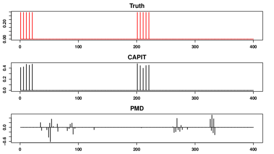
Figure 1: Visualization of the simulation results of estimating $(\theta,\eta)$ for a replicate from Scenario II in Section 5.2 when $p=200$ and $n=500$. The $\{1,2,...,200\}$-th coordinates represent $\theta$ and the $\{201,202,...,400\}$-th coordinates represent $\eta$.

A closely related problem is the principal component analysis (PCA) (Hotelling, 1933). In high-dimensional setting, sparse PCA is studied in Johnstone and Lu (2009), Ma (2013) and Cai et al. (2012). However, the PCA and CCA problems are fundamentally different. With the characterization of covariance structure in (3), such difference becomes clear. We illustrate the simplest rank-one case. Assuming the correlation rank $r$ in (3) is one, the covariance structure is reduced to

$$\Sigma_{12}=\lambda\Sigma_{1}\theta\eta^{T}\Sigma_{2}.$$ (4)

We refer to (4) as the Single Correlation Pair (SCP) model. In the PCA literature, the corresponding rank-one model is called the single-spike model. Its covariance structure can be written as

$$\Sigma=\lambda\theta\theta^{T}+I,$$ (5)

where $\theta$ is the principal direction of the random variable. A comparison of (4) and (5) reveals that estimation of the CCA is more involved than that of the PCA because of the presence of the nuisance parameters $(\Sigma_{1},\Sigma_{2})$, and the difficulty of estimating covariance matrices and precision matrices is known in high-dimensional statistics (Cai and Zhou, 2012; Ren et al., 2013). In the sparse PCA setting, the absence of nuisance parameter in (5) leads to algorithms directly applied on the sample covariance matrix $\hat{\Sigma}$, and the corresponding theoretical analysis is more tractable. In contrast, in the sparse CCA setting, not only do we need to adapt to the underlying sparsity of $(\theta,\eta)$, but we also need to adapt to the unknown covariance structure $(\Sigma_{1},\Sigma_{2})$. We are going to show in Section 4 how various structures of $(\Sigma_{1},\Sigma_{2})$ influence the convergence rate of the proposed method.

In addition, we demonstrate the CAPIT method by a real data example. We apply the proposed method to the data arising in the field of cancer genomics where methylation and gene expression are profiled for the same group of breast cancer patients. The method explicitly takes into account the sparse graphical model structure among genes. Interestingly, we identify methylation probes that are associated with genes that are previously characterized as prognosis signatures of the metastasis of breast cancer. This example suggests the proposed method provides a reasonable framework for exploratory and interpretive analysis of multiple datasets in high-dimensional settings.

The contributions in the paper are two-fold. First, we characterize the sparse CCA problem by proposing the probabilistic model and establish the minimax lower bound under certain sparsity class. Second, we propose the CAPIT method to adapt to both sparsity of the canonical direction and the nuisance structure. The CAPIT procedure is computationally efficient and attains optimal rate of convergence under various conditions. The paper is organized as follows. We first provide a full characterization of the sparse CCA model in Section 2. The CAPIT method and its associated algorithms are presented in Section 3. Section 4 is devoted to a theoretical analysis of our method. This section also presents the minimax lower bound. Section 5 and Section 6 investigate the numerical performance of our procedure by simulation studies and a real data example. The proof of the main theorem, Theorem 4.1, is gathered in Section 7. The proofs of all technical lemmas and Theorem 4.2 are gathered in Appendix.

1.1 Notations

For a matrix $A=(a_{ij})$, we use $||A||$ to denote its largest singular value and call it the spectral norm of $A$. The Frobenius norm is defined as $||A||=\sqrt{\sum_{ij}a_{ij}^{2}}$. The matrix $l_{1}$ norm is defined as $||A||_{l_{1}}=\max_{j}\sum_{i}|a_{ij}|$. The norm $||\cdot||$, when applied to a vector, is understood as the usual Euclidean $l_{2}$ norm. For any two real numbers $a$ and $b$, we use notations $a\vee b=\max(a,b)$ and $a\wedge b=\min(a,b)$. Other notations will be introduced along with the text.

2 The Sparse CCA Model

Let $X\in\mathbb{R}^{p_{1}}$ and $Y\in\mathbb{R}^{p_{2}}$ be two centered multivariate random vectors with dimension $p_{1}$ and $p_{2}$ respectively. Write the covariance matrix of $(X^{T},Y^{T})^{T}$ as follows,

$$\mbox{\rm Cov}\begin{pmatrix}X\\ Y\end{pmatrix}=\begin{pmatrix}\Sigma_{1}&\Sigma_{12}\\ \Sigma_{21}&\Sigma_{2}\end{pmatrix},$$

where $\Sigma_{1}$ is the covariance matrix of $X$ with $\Sigma_{1}=\mathbb{E}XX^{T}$, $\Sigma_{2}$ is the covariance matrix of $Y$ with $\Sigma_{2}=\mathbb{E}YY^{T}$, and $\Sigma_{21}=\Sigma_{12}^{T}$ the covariance structure between $X$ and $Y$ with $\Sigma_{12}=\Sigma_{21}^{T}=\mathbb{E}XY^{T}$. The canonical directions $\theta\in\mathbb{R}^{p_{1}}$ and $\eta\in\mathbb{R}^{p_{2}}$ are solutions of

$$\max_{a\in\mathbb{R}^{p_{1}},b\in\mathbb{R}^{p_{2}}}\frac{a^{T}\Sigma_{12}b}{\sqrt{a^{T}\Sigma_{1}a}\sqrt{b^{T}\Sigma_{2}b}}.$$ (6)

where we assume $\Sigma_{1}$ and $\Sigma_{2}$ are invertible and $\Sigma_{12}$ is nonzero such that the maximization problem is not degenerate. Notice when $(\theta,\eta)$ is the solution of (6), $(\sigma_{1}\theta,\sigma_{2}\eta)$ is also the solution with arbitrary scalars $(\sigma_{1},\sigma_{2})$ satisfying $\sigma_{1}\sigma_{2}>0$. To achieve identifiability up to a sign, (6) can be reformulated into the following optimization problem.

$$\mbox{\rm maximize }a^{T}\Sigma_{12}b,\quad\mbox{\rm subject to }a^{T}\Sigma_{1}a=1\quad\mbox{\rm and}\quad b^{T}\Sigma_{2}b=1.$$ (7)

Proposition 2.1

When $\Sigma_{12}$ is of rank $1$, the solution (up to sign jointly) of Equation (7) is $\left(\theta,\eta\right)$ if and only if the covariance structure between $X$ and $Y$ can be written as

$$\Sigma_{12}=\lambda\Sigma_{1}\theta\eta^{T}\Sigma_{2},$$

where $0<\lambda\leq 1,$ $\theta^{T}\Sigma_{1}\theta=1$ and $\eta^{T}\Sigma_{2}\eta=1$. In other words, the correlation between $a^{T}X$ and $b^{T}Y$ are maximized by $\mbox{\rm corr}(\theta^{T}X,\eta^{T}Y)$, and $\lambda$ is the canonical correlation between $X$ and $Y$.

The Proposition above is just an elementary consequence of SVD after transforming the parameters $\theta$ and $\eta$ into $\Sigma_{1}^{1/2}\theta$ and $\Sigma_{2}^{1/2}\eta$ respectively. For the reasons of space, the proof is omitted. For general $\Sigma_{12}$ with rank $r\geq 1,$ it’s a routine extension to see that the unique (up to sign jointly) solution of Equation (7) is $\left(\theta_{1},\eta_{1}\right)$ if and only if the covariance structure between $X$ and $Y$ can be written as

$$\Sigma_{12}=\Sigma_{1}\left(\sum_{i=1}^{r}\lambda_{i}\theta_{i}\eta_{i}^{T}\right)\Sigma_{2},$$

where $\lambda_{i}$ decreases $\lambda_{1}>\lambda_{2}\geq\ldots\geq\lambda_{r}>0$, $\left\{\theta_{i}\right\}$ and $\left\{\eta_{i}\right\}$ are orthonormal w.r.t. metric $\Sigma_{1}$ and $\Sigma_{2}\$respectively. i.e. $\theta_{i}^{T}\Sigma_{1}\theta_{j}=\mathbb{I}\{i=j\}$ and $\eta_{i}^{T}\Sigma_{2}\eta_{j}=\mathbb{I}\{i=j\}$.

Inspired by (7), we propose a probabilistic model of $(X,Y)$, so that the canonical directions $(\theta,\eta)$ are explicitly modeled in the joint distribution of $(X,Y)$.

The Single Canonical Pair Model

$$\begin{pmatrix}X\\ Y\end{pmatrix}\sim N\begin{pmatrix}\begin{pmatrix}0\\ 0\end{pmatrix},\begin{pmatrix}\Sigma_{1}&\lambda\Sigma_{1}\theta\eta^{T}\Sigma_{2}\\ \lambda\Sigma_{2}\eta\theta^{T}\Sigma_{1}&\Sigma_{2}\end{pmatrix}\end{pmatrix},$$ (8)

with $\Sigma_{1}\succ 0$, $\Sigma_{2}\succ 0$, $\theta^{T}\Sigma_{1}\theta=1$, $\eta^{T}\Sigma_{2}\eta=1$ and $0<\lambda\leq 1$.

Just as the single-spike model in PCA (Tipping and Bishop, 1999; Johnstone and Lu, 2009), the model (8) explicitly models $(\lambda,\theta,\eta)$ in the form of the joint distribution of $(X,Y)$. Besides, it can be generalized to multiple canonical-pair structure as in the multi-spike model (Birnbaum et al., 2012). On the other hand, it is fundamentally different from the single-spike model, because $(\Sigma_{1},\Sigma_{2})$ are typically unknown, so that estimating $(\theta,\eta)$ is much harder than estimating the spike in PCA. Even when both $\Sigma_{1}$ and $\Sigma_{2}$ are identity and $\Sigma_{12}=\lambda\theta\eta^{T}$, it cannot be reduced into the form of spike model. Bach and Jordan (2005) also proposed a statistical model for studying CCA in a probabilistic setting. Under their model, the data has a latent variable representation. It can be shown that the model we propose is equivalent to theirs in the sense that both can be written into the form of the other. The difference is that we explicitly model the canonical directions $(\theta,\eta)$ in the covariance structure for sparse CCA.

3 Methodology

In this section, we introduce the CAPIT algorithm to estimate the sparse canonical direction pair $(\theta,\eta)$ in the single canonical pair model in details. We start with the main part of the methodology in Section 3.1, an iterative thresholding algorithm, requiring an initializer and consistent estimators of precision matrices (nuisance parameters). Then in Section 3.2 we introduce a coordinate thresholding algorithm to provide a consistent initializer. Finally, in Section 3.3 rate-optimal estimators of precision matrices are reviewed over various settings.

The procedure is motivated by the power method, a standard technique to compute the leading eigenvector of a given symmetric matrix $S$ (Golub and Van Loan, 1996). Let $S$ be a $p\times p$ symmetric matrix. We compute its leading eigenvector. Starting with a vector $v^{(0)}$ non-orthogonal to the leading eigenvector, the power method generates a sequence of vectors $v^{(i)}$, $i=1,2,\ldots,$ by alternating the multiplication step $w^{(i)}=Sv^{(i-1)}$ and the normalization step $v^{(i)}=w^{(i)}/\left\|w^{(i)}\right\|$ until convergence. The limit of the sequence, denoted by $v^{(\infty)}$, is the leading eigenvector. The power method can be generalized to compute the leading singular vectors of any $p_{1}\times p_{2}$ dimensional rectangular matrix $M$. Suppose the SVD of a rank $d$ matrix $M$ is $M=UDV^{T}$, where $D$ is the $d$ dimensional diagonal matrix with singular values on the diagonal. Suppose we are given an initial pair $\left(u^{(0)},v^{(0)}\right)$, non-orthogonal to the leading singular vectors. To compute the leading singular vectors, power method alternates the following steps until $\left(u^{(0)},v^{(0)}\right)$ converges to $\left(u^{(\infty)},v^{(\infty)}\right)$, which are the left and right leading singular vectors.

1. Right Multiplication: $w_{l}^{(i)}=Mv^{(i-1)},$

2. Left Normalization: $u^{(i)}=w_{l}^{(i)}/\left\|w_{l}^{(i)}\right\|,$

3. Left Multiplication: $w_{r}^{(i)}=u^{(i)}M,$

4. Right Normalization: $v^{(i)}=w_{r}^{(i)}/\left\|w_{r}^{(i)}\right\|.$

Our goal is to estimate the canonical direction pair $\left(\theta,\eta\right)$. The power method above motivates us to find a matrix $\hat{A}$ close to $\lambda\theta\eta^{T}$ of which $\left(\theta/\left\|\theta\right\|,\eta/\left\|\eta\right\|\right)$ is the leading pair of singular vectors. Note that the covariance structure is $\Sigma_{12}=\lambda\Sigma_{1}\theta\eta^{T}\Sigma_{2}$. Suppose we know the marginal covariance structures of $X$ and $Y$, i.e. $\Omega_{1}=\Sigma_{1}^{-1}$ and $\Omega_{2}=\Sigma_{2}^{-1}$ are given, it is very natural to consider $\Omega_{1}\hat{\Sigma}_{12}\Omega_{2}$ as the target matrix, where $\hat{\Sigma}_{12}$ is the sample cross-covariance between $X$ and $Y$. Unfortunately, the covariance structures $\Omega_{1}$ and $\Omega_{2}$ are unknown as nuisance parameters, but a rate-optimal estimator of $\Omega_{j}$ ($j=1,2$) usually can be obtained under various assumptions on the covariance or precision structures of $X$ and $Y$ in many high-dimensional settings. In literature, some commonly used structures are sparse precision matrix, sparse covariance matrix, bandable covariance matrix and Toeplitz covariance matrix structures. Later we will discuss the estimators of the precision matrices and their influences to the final estimation error of canonical direction pair $\left(\theta,\eta\right)$.

We consider the idea of data splitting. Suppose we have $2n$ i.i.d. copies $(X_{i},Y_{i})_{1\leq i\leq 2n}$. We use the first half to compute the sample covariance $\hat{\Sigma}_{12}=\frac{1}{n}\sum_{i=1}^{n}X_{i}Y_{i}^{T}$, and use the second half to estimate the precision matrices by $\hat{\Omega}_{1}$ and $\hat{\Omega}_{2}$. Hence the matrix $\hat{A}=\hat{\Omega}_{1}\hat{\Sigma}_{12}\hat{\Omega}_{2}$ is available to us. The reason for data splitting is that we can write the matrix $\hat{A}$ in an alternative form. That is,

$$\hat{A}=\frac{1}{n}\sum_{i=1}^{n}\tilde{X}_{i}\tilde{Y}_{i}^{T},$$

where $\tilde{X}_{i}=\hat{\Omega}_{1}X_{i}$ and $\tilde{Y}_{i}=\hat{\Omega}_{2}Y_{i}$ for all $i=1,...,n$. Conditioning on $(X_{n+1},Y_{n+1}),...,(X_{2n},Y_{2n})$, the transformed data $(\tilde{X}_{i},\tilde{Y}_{i})_{1\leq i\leq n}$ are still independently identically distributed. This feature allows us to explore some useful concentration results in the matrix $\hat{A}$ to prove theoretical results. Conditioning on the second half of data, the expectation of $\hat{A}$ is $\lambda\alpha\beta^{T}$, where $\alpha=\hat{\Omega}_{1}\Sigma_{1}\theta$ and $\beta=\hat{\Omega}_{2}\Sigma_{2}\eta$. Therefore, the method we develop is targeted at $(\alpha,\beta)$ instead of $(\theta,\eta)$. However, as long as the estimators $(\hat{\Omega}_{1},\hat{\Omega}_{2})$ are accurate in the sense that

$$||\alpha-\theta||\vee||\beta-\eta||=||(\hat{\Omega}_{1}\Sigma_{1}-I)\theta||\vee||(\hat{\Omega}_{2}\Sigma_{2}-I)\eta||$$

is small, the final rate of convergence is also small.

If we naively apply the power method above to $\hat{A}=\hat{\Omega}_{1}\hat{\Sigma}_{12}\hat{\Omega}_{2}$ in high-dimensional setting, the estimation variance accumulated across all $p_{1}$ and $p_{2}$ coordinates of left and right singular vectors goes very large and it is possible that we can never obtain a consistent estimator of the space spanned by the singular vectors. Johnstone and Lu (2009) proved that when $p/n\nrightarrow 0$, the leading eigenspace estimated directly from the sample covariance matrix can be nearly orthogonal to the truth under the PCA setting in which $\hat{A}$ is the sample covariance matrix with dimension $p_{1}=p_{2}=p$. Under the sparsity assumption of $\left(\theta,\eta\right)$, a natural way of reducing the estimation variance is to only estimate those coordinates with large values in $\theta$ and $\eta$ respectively and simply estimate the rest coordinates by zero. Although bias is caused by this thresholding idea, in the end the variance reduction dominates the biased inflation and this trade-off minimizes the estimation error to the optimal rate. The idea of combining the power method and the iterative thresholding procedure leads to the algorithm in the next section which was also proposed by Yang et al. (2013) for a general data matrix $\hat{A}$ without a theoretical analysis.

3.1 Iterative Thresholding

We incorporate the thresholding idea into ordinary power method above for SVD by adding a thresholding step after each right and left multiplication steps before normalization. The thresholding step kills those coordinates with small magnitude to zero and keep or shrink the rest coordinates through a thresholding function $T\left(a,t\right)$ in which $a$ is a vector and $t$ is the thresholding level. In our theoretical analysis, we assume that $T\left(a,t\right)=\Big{(}a_{k}\mathbb{I}\{|a_{k}|\geq t\}\Big{)}$ is the hard-thresholding function, but any function serves the same purpose in theory as long as it satisfies (i) $\left|T\left(a,t\right)_{k}-a_{k}\right|\leq t$ and (ii) $T\left(a,t\right)_{k}=0$ whenever $\left|a_{k}\right|<t$. Therefore the thresholding function can be hard-thresholding, soft-thresholding or SCAD (Fan and Li, 2001). The algorithm is summarized below.

Input: Sample covariance matrices $\hat{\Sigma}_{12}$;

Estimators of precision matrix $\hat{\Omega}_{1},\hat{\Omega}_{2}$;

Initialization pair $\alpha^{(0)},\beta^{(0)}$;

Thresholding level $\gamma_{1},\gamma_{2}$.

Output: Canonical direction estimator $\alpha^{(\infty)},\beta^{(\infty)}$.

Set $\hat{A}=\hat{\Omega}_{1}\hat{\Sigma}_{12}\hat{\Omega}_{2}$;

repeat

       Right Multiplication: $w^{l,(i)}=\hat{A}\beta^{(i-1)}$;

       Left Thresholding: $w_{th}^{l,(i)}=T\left(w^{l,(i)},\gamma_{1}\right)$;

       Left Normalization: $\alpha^{(i)}=w_{th}^{l,(i)}/\left\|w_{th}^{l,(i)}\right\|$;

       Left Multiplication: $w^{r,(i)}=\alpha^{(i)}\hat{A}$;

       Right Thresholding: $w_{th}^{r,(i)}=T\left(w^{r,(i)},\gamma_{2}\right)$;

       Right Normalization: $\beta^{(i)}=w_{th}^{r,(i)}/\left\|w_{th}^{r,(i)}\right\|$;

until Convergence of $\alpha^{(i)}$ and $\beta^{(i)}$;

Algorithm 1 CAPIT: Iterative Thresholding

Remark 3.1

In Algorithm 1, we don’t provide specific stopping rule such as that the difference between successive iterations is small enough. For the single canonical pair model, we are able to show in Section 4 that the convergence is achieved in just one step. The intuition is simple: when $A$ is of exact rank one, we can simply obtain the left singular vector via right multiplying $A$ by any vector non-orthogonal to the right singular vector. Although in the current setting $\hat{A}$ is not a rank one matrix, the effect caused from the second singular value in nature does not change the statistical performance of our final estimator.

Remark 3.2

The thresholding level $(\gamma_{1},\gamma_{2})$ are user-specified. Theoretically, they should be set at the level $O\Big{(}\sqrt{\frac{\log(p_{1}\vee p_{2})}{n}}\Big{)}$. In Section 7.2, we present a fully data-driven $(\gamma_{1},\gamma_{2})$ along with the proof.

Remark 3.3

The estimator $(\alpha^{(\infty)},\beta^{(\infty)})$ does not directly estimate $(\theta,\eta)$ because the former are unit vectors while the later satisfies $\theta^{T}\Sigma_{1}\theta=\eta^{T}\Sigma_{2}\eta=1$. We are going to prove they are almost in the same direction by considering the loss function $|\sin\angle(a,b)|^{2}$ in Johnstone and Lu (2009). Details are presented in Section 4.

Remark 3.4

The estimators of precision matrices $\hat{\Omega}_{1}$ and $\hat{\Omega}_{2}$ depend on the second half of the data and the estimator $\hat{\Sigma}_{12}$ depends on the first half of the data. In practice, after we apply Algorithm 1, we will swap the two parts of the data and use the first half to get $\hat{\Sigma}_{12}$ and the second half to obtain $\hat{\Omega}_{1},\hat{\Omega}_{2}$. Then, Algorithm 1 is run again on the new estimators. The final estimator can be calculated through averaging the two. More generally, we can do sample splitting many times and take an average as Bagging, which is often used to improve the stability and accuracy of machine learning algorithms.

3.2 Initialization by Coordinate Thresholding

In Algorithm 1, we need to provide an initializer $\left(\alpha^{(0)},\beta^{(0)}\right)$ as input. We generate a sensible initialization in this section which is similar to the “diagonal thresholding” sparse PCA method proposed by Johnstone and Lu (2009). Specifically, we apply a thresholding step to pick index sets $B_{1}$ and $B_{2}$ of the coordinates of $\theta$ and $\eta$ respectively. Those index sets can be thought as strong signals. Then a standard SVD is applied on the submatrix of $\hat{A}$ with rows and columns indexed by $B_{1}$ and $B_{2}$. The dimension of this submatrix is relatively low such that the SVD on it is fairly accurate. The leading pair of singular vectors is of dimension $\left|B_{1}\right|$ and $\left|B_{2}\right|$, where $\left|\cdot\right|$ denotes the cardinality. In the end, we zero-pad the leading pair of singular vectors into dimension $p_{1}$ and $p_{2}$ respectively to provide our initializer $\left(\alpha^{(0)},\beta^{(0)}\right)$. The algorithm is summarized in Algorithm 2.

Input: Sample covariance matrices $\hat{\Sigma}_{12}$;

Estimators of precision matrix $\hat{\Omega}_{1},\hat{\Omega}_{2}$;

Thresholding level $t_{ij}$.

Output: Initializer $\alpha^{(0)}$ and $\beta^{(0)}$.

Set $\hat{A}=\hat{\Omega}_{1}\hat{\Sigma}_{12}\hat{\Omega}_{2}$ ;

1 Coordinate selection: pick the index sets $B_{1}$ and $B_{2}$ of the coordinates of $\theta$ and $\eta$ respectively as follows, $B_{1}=\left\{i,\max_{j}\left|\hat{a}_{ij}\right|/t_{ij}\geq\sqrt{\frac{\log p_{1}}{n}}\right\},B_{2}=\left\{j,\max_{i}\left|\hat{a}_{ij}\right|/t_{ij}\geq\sqrt{\frac{\log p_{2}}{n}}\right\}$;

2 Reduced SVD: compute the leading pair of singular vectors $\left(\alpha^{(0),B_{1}},\beta^{(0),B_{2}}\right)$ on the submatrix $\hat{A}_{B_{1},B_{2}}$;

3 Zero-Padding procedure: construct the initializer $\left(\alpha^{(0)},\beta^{(0)}\right)$ by zero-padding $\left(\alpha^{(0),B_{1}},\beta^{(0),B_{2}}\right)$ on index sets $B_{1}^{c}$ and $B_{2}^{c}$ respectively, $\alpha_{B_{1}}^{(0)}=\alpha^{(0),B_{1}},\alpha_{B_{1}^{c}}^{(0)}=0,\beta_{B_{2}}^{(0)}=\beta^{(0),B_{2}},\beta_{B_{2}^{c}}^{(0)}=0.$

Algorithm 2 CAPIT: Initialization by Coordinate Thresholding

The thresholding level $t_{ij}$ in Algorithm 2 is a user specified constant and allowed to be adaptive to each location $\left(i,j\right)$. The theoretical data-driven constant for each $t_{ij}$ is provided in Section 7.2. It is clear the initializer is not unique since if $\left(\alpha^{(0)},\beta^{(0)}\right)$ serves as the output, $\left(-\alpha^{(0)},-\beta^{(0)}\right)$ is also a solution of Algorithm 2. However either pair works as an initializer and provides the same result because in the end we estimate the space spanned by leading pair of singular vectors.

3.3 Precision Estimation

Algorithms 1 and 2 require precision estimators $\hat{\Omega}_{1}$ and $\hat{\Omega}_{2}$ to start with. As we mentioned, we apply the second half of the data to estimate the precision matrix $\hat{\Omega}_{1}$ and $\hat{\Omega}_{2}$. In this section, we discuss four commonly assumed covariance structures of $X$ itself and provide corresponding estimators. We apply the same procedure to $Y$.

3.3.1 Sparse Precision Matrices

Precision matrix is closely connected to the undirected graphical model which is a powerful tool to model the relationships among a large number of random variables in a complex system. It is well known that recovering the structure of an undirected Gaussian graph is equivalent to recovering the support of the precision matrix. In this setting, it is natural to impose sparse graph structure among variables in $X$ by assuming sparse precision matrices $\Omega_{1}$. Many algorithms targeting on estimating sparse precision matrix were proposed in literature. See, e.g. Meinshausen and Bühlmann (2006), Friedman et al. (2008), Cai et al. (2011) and Ren et al. (2013). In the current paper, we apply the CLIME method to estimate $\Omega_{1}$. For details of the algorithm, we refer to Cai et al. (2011).

3.3.2 Bandable Covariance Matrices

Motivated by applications in time series, where there is a natural “order” on the variables, the bandable class of covariance matrices was proposed by Bickel and Levina (2008a). In this setting, we assume that $\sigma_{ij}$ decay to zero at certain rate as $\left|i-j\right|$ goes away from the diagonal. Usually regularizing the sample covariance matrix by banding or tapering procedures were applied in literature. We apply the tapering method proposed in Cai et al. (2010). Let $\omega=(\omega_{m})_{0\leq m\leq p-1}$ be a weight sequence with $\omega_{m}$ given by

$$\mathbb{\omega}_{m}=\left\{\begin{array}[]{cc}1,&\mbox{\rm when }m\leq k/2\\ 2-\frac{2m}{k},&\mbox{\rm when }k/2<m\leq k\\ 0,&\mbox{\rm Otherwise}\end{array}\right.,$$ (9)

where $k$ is the bandwidth. The tapering estimator $\hat{\Sigma}_{1}$ of the covariance matrix of $X$ is given by $\hat{\Sigma}_{1}=(\hat{\sigma}_{ij}^{sam}\mathbb{\omega}_{\left|i-j\right|})$, where $\hat{\sigma}_{ij}^{sam}$ is the $(i,j)$-th entry of the sample covariance matrix. The bandwidth $k$ is chosen through cross-validation in practice. An alternative adaptive method was proposed by Cai and Yuan (2012). In the end, our estimator is $\hat{\Omega}_{1}=\hat{\Sigma}_{1}^{-1}$.

3.3.3 Toeplitz Covariance Matrices

Toeplitz matrix is the symmetric matrix that the entries are constant along the off-diagonals which are parallel to the main diagonal. Class of Toeplitz covariance matrices arises naturally in the analysis of stationary stochastic processes. If $X$ is a stationary process with autocovariance sequence $(\alpha_{m})\equiv\left(\alpha_{0},\alpha_{1},\cdots,\alpha_{p-1},\cdots\right),$ then the covariance matrix $\Sigma_{1}=\left(\sigma_{ij}\right)_{p_{1}\times p_{1}}$ has a Toeplitz structure $\sigma_{ij}=\alpha_{\left|i-j\right|}$. In this setting, it is natural to assume certain rate of decay of the autocovariance sequence. We apply the following tapering method proposed in Cai et al. (2013). Define $\tilde{\sigma}_{m}={\frac{1}{p-m}}\sum_{s-t=m}\hat{\sigma}_{st}^{sam},$ the average of sample covariance along each off-diagonal. Then the tapering estimator $\hat{\Sigma}_{1}=\left(\hat{\sigma}_{st}\right)$ with bandwidth $k$ is defined as $\hat{\sigma}_{st}=\omega_{|s-t|}\tilde{\sigma}_{|s-t|},$ where $\omega=(\omega_{m})_{0\leq m\leq p-1}$ is defined in Equation (9). In practice, we pick bandwidth $k$ using cross-validation. The final estimator of $\Omega_{1}$ is then defined as $\hat{\Omega}_{1}=\hat{\Sigma}_{1}^{-1}$.

3.3.4 Sparse Covariance Matrices

In many applications, there is no natural order on the variables like we assumed in bandable and Toeplitz covariance matrices. In this setting, permutation-invariant estimators are favored and general sparsity assumption is usually imposed on the whole covariance matrix, i.e. most of entries in each row/column of covariance matrix are zero or negligible. We apply a hard thresholding procedure proposed in Bickel and Levina (2008b) under this assumption. Again, let $\hat{\sigma}_{ij}^{sam}$ be the $(i,j)$-th entry of the sample covariance matrix of $X$. The thresholding estimator $\hat{\Sigma}_{1}=\left(\hat{\sigma}_{st}\right)$ is given by $\hat{\sigma}_{ij}=\hat{\sigma}_{ij}^{sam}I\left(|\hat{\sigma}_{ij}^{sam}|\geq\gamma\sqrt{\frac{\log p}{n}}\right)$ for some constant $\gamma$ which is chosen through cross-validation. In the end, our estimator is $\hat{\Omega}_{1}=\hat{\Sigma}_{1}^{-1}$.

4 Statistical Properties and Optimality

In this section, we present the statistical properties and optimality of our proposed estimator. We first present the convergence rates of our procedure, and then we provide a minimax lower bound for a wide range of parameter spaces. In the end, we can see when estimating the nuisance parameters is not harder than estimating canonical direction pair, the rates of convergence match the minimax lower bounds. Hence we obtain the minimax rates of convergence for a range of sparse parameter spaces.

4.1 Convergence Rates

Notice that our model is fully determined by the parameter $(\Sigma_{1},\Sigma_{2},\lambda,\theta,\eta)$, among which we are interested in estimating $(\theta,\eta)$. To achieve statistical consistency, we need some assumptions on the interesting part $(\theta,\eta)$ and nuisance part $(\Sigma_{1},\Sigma_{2},\lambda)$.

Assumption A - Sparsity Condition on $(\theta,\eta)$:

We assume $\theta$ and $\eta$ are in the weak $l_{q}$ ball, with $0\leq q\leq 2$. i.e.

$$\left|\theta_{\left(k\right)}\right|^{q}\leq s_{1}k^{-1}\mbox{\rm, }\left|\eta_{\left(k\right)}\right|^{q}\leq s_{2}k^{-1}\mbox{\rm,}$$

where $\theta_{\left(k\right)}$ is the $k$-th largest coordinate by magnitude. Let $p=p_{1}\vee p_{2}$ and $s=s_{1}\vee s_{2}$. The sparsity levels $s_{1}$ and $s_{2}$ satisfy the following condition,

$$s=o\left(\left(\frac{n}{\log p}\right)^{\frac{1}{2}-\frac{q}{4}}\right)\mbox{\rm.}$$ (10)

Remark 4.1

In general, we can allow $\theta$ to be in the weak $l_{q_{1}}$ ball and $\eta$ to be in the weak $l_{q_{2}}$ ball with $q_{1}\neq q_{2}$. In that case, we require $s_{i}=o\left(\left(n/\log p\right)^{\frac{1}{2}-\frac{q_{i}}{4}}\right)$ for $i=1,2$. There is no fundamental difference in the analysis and procedures. For simplicity, in the paper we only consider $q_{1}=q_{2}$.

Assumption B - General Conditions on $(\Sigma_{1},\Sigma_{2},\lambda)$:

1. We assume there exist constants $w$ and $W$, such that

   $$0<w\leq\lambda_{\min}(\Sigma_{i})\leq\lambda_{\max}(\Sigma_{i})\leq W<\infty,$$

   for $i=1,2$.

2. In order that the signals do not vanish, we assume the canonical correlation is bounded below by a positive constant $C_{\lambda}$, i.e. $0<C_{\lambda}\leq\lambda\leq 1$.

3. Moreover, we require that estimators $(\hat{\Omega}_{1},\hat{\Omega}_{2})$ are consistent in the sense that

   $$\xi_{\Omega}=||\hat{\Omega}_{1}\Sigma_{1}-I||\vee||\hat{\Omega}_{2}\Sigma_{2}-I||=o(1),$$ (11)

   with probability at least $1-O(p^{-2})$.

Loss Function

For two vectors $a,b$, a natural way to measure the discrepancy of their directions is the sin of the angle $|\sin\angle(a,b)|$, see Johnstone and Lu (2009). We consider the loss function $L(a,b)^{2}=2|\sin\angle(a,b)|^{2}$. It is easy to calculate that

$$L(a,b)=\left\|\frac{aa^{T}}{||a||^{2}}-\frac{bb^{T}}{||b||^{2}}\right\|_{F}.$$

The convergence rate of the CAPIT procedure is presented in the following theorem.

Theorem 4.1

Assume the Assumptions A and B above hold. Let $(\alpha^{(k)},\beta^{(k)})$ be the sequence from Algorithm 1, with the initializer $(\alpha^{(0)},\beta^{(0)})$ calculated by Algorithm 2. The thresholding levels are

$$t_{ij},\quad\gamma_{1}=c_{1}\sqrt{\frac{\log p}{n}},\quad\gamma_{2}=c_{2}\sqrt{\frac{\log p}{n}},$$

for sufficiently large constants $(t_{ij},c_{1},c_{2})$. Then with probability at least $1-O(p^{-2})$, we have

$$L(\alpha^{(k)},\theta)^{2}\vee L(\beta^{(k)},\eta)^{2}\leq C\left(s\Big{(}\frac{\log p}{n}\Big{)}^{1-q/2}+||(\hat{\Omega}_{1}\Sigma_{1}-I)\theta||^{2}\vee||(\hat{\Omega}_{2}\Sigma_{2}-I)\eta||^{2}\right),$$

for all $k=1,2,...,K$ with $K=O(1)$ and some constant $C>0$.

Remark 4.2

Notice the thresholding levels depend on some unknown constants $(t_{ij},c_{1},c_{2})$. This is for the simplicity of presentation. A more involved fully data-driven choice of thresholding levels are presented in Section 7.2 along with the proof.

The upper bound in Theorem 4.1 implies that the estimation of nuissance parameters $\hat{\Omega}_{i}$ affect the estimation canonical directions in terms of $||(\hat{\Omega}_{1}\Sigma_{1}-I)\theta||^{2}$ and $||(\hat{\Omega}_{2}\Sigma_{2}-I)\eta||^{2}$. In Section 3.3, we discussed four different settings in which certain structure assumptions are imposed on the nuance parameters $\Omega_{1}$ and $\Omega_{2}$. In the literature, optimal rates of convergence in estimating ${\Omega}_{i}$ under spectral norm have been established and can be applied here in each of the four settings, noting that $||(\hat{\Omega}_{1}\Sigma_{1}-I)\theta||^{2}\leq||(\hat{\Omega}_{1}-\Omega_{1})||^{2}\left\|\Sigma_{1}\theta\right\|^{2}\leq W||(\hat{\Omega}_{1}-\Omega_{1})||^{2}$. Due to the limited space, we only discuss one setting in which we assume sparse precision matrix structure on $\Omega_{i}$.

Besides the first general condition in Assumption B, we assume each row/column of $\Omega_{i}$ is in a weak $l_{q_{0}}$ ball with $0\leq q_{0}\leq 1$. i.e. $\Omega_{i}\in\mathcal{G}_{q_{0}}\left(s_{0},p_{i}\right)$ for $i=1,2$, where

$$\mathcal{G}_{q_{0}}\left(s_{0},p\right)=\left\{\Omega=\left(\omega_{ij}\right)_{p\times p}:\max_{j}\left|\omega_{j(k)}\right|^{q_{0}}\leq s_{0}k^{-1}\mbox{\rm for all }k\right\},$$

and the matrix $l_{1}$ norm of $\Omega_{i}$ is bounded by some constant $\left\|\Omega_{i}\right\|_{l_{1}}\leq w^{-1}$. The notation $\omega_{j(k)}$ means the $k$-th largest coordinate of $j$-th row of $\Omega$ in magnitude. Recall that $p=p_{1}\vee p_{2}$. Under the assumptions that $s_{0}^{2}=O\left(\left(n/\log p\right)^{1-q_{0}}\right)$, Theorem 2 in Cai et al. (2011) implies that CLIME estimator with an appropriate tuning parameter attaining the following rate of convergence $||(\hat{\Omega}_{1}\Sigma_{1}-I)\theta||^{2}$ with probability at least $1-O\left(p^{-2}\right),$

$$||(\hat{\Omega}_{1}\Sigma_{1}-I)\theta||^{2}\leq W||(\hat{\Omega}_{1}-\Omega_{1})||^{2}\leq Cs_{0}^{2}\left(\frac{\log p}{n}\right)^{1-q_{0}}\mbox{\rm.}$$

Therefore we obtain the following corollary.

Corollary 4.1

Assume the Assumptions A and B holds, $\Omega_{i}\in\mathcal{G}_{q_{0}}\left(s_{0},p_{i}\right)$ $i=1,2$, $\left\|\Omega_{i}\right\|_{l_{1}}\leq w^{-1}$ and $s_{0}^{2}=O\left(\left(n/\log p\right)^{1-q_{0}}\right)$. Let $(\alpha^{(k)},\beta^{(k)})$ be the sequence from Algorithm 1, with the initializer $(\alpha^{(0)},\beta^{(0)})$ calculated by Algorithm 2 and $\hat{\Omega}_{i}$ obtained by applying CLIME procedure in Cai et al. (2011). The thresholding levels are the same as those in Theorem 4.1. Then with probability at least $1-O(p^{-2})$, we have

$$L(\alpha^{(k)},\theta)^{2}\vee L(\beta^{(k)},\eta)^{2}\leq C\left(s\Big{(}\frac{\log p}{n}\Big{)}^{1-q/2}+s_{0}^{2}\Big{(}\frac{\log p}{n}\Big{)}^{1-q_{0}}\right),$$

for all $k=1,2,...,K$ with $K=O(1)$ and some constant $C>0$.

Remark 4.3

It can be seen from the analysis that similar upper bounds hold in Corollary 4.1 with probability $1-O(p^{-h})$ by picking different thresholding constants in Algorithms 1, 2 and CLIME procedure for any $h>0$. Assuming that $n=o(p^{h}),$ the boundedness of loss function implies that Corollary 4.1 is valid in the risk sense.

4.2 Minimax Lower Bound

In this section, we establish a minimax lower bound in a simpler setting in which we know the covariance matrices $\Sigma_{1}$ and $\Sigma_{2}$. We assume $\Sigma_{i}=I_{p_{i}\times p_{i}}$ for $i=1,2$ for simplicity. Otherwise, we can transfer the data accordingly and make $\Sigma_{i}=I_{p_{i}\times p_{i}}$. The purpose of establishing this minimax lower bound is to measure the difficulty of estimation problems in sparse CCA model. In view of the upper bound given in Theorem 4.1 by the iterative thresholding procedure Algorithms 1 and 2, this lower bound is minimax rate optimal under conditions that estimating nuisance precision matrices is not harder than estimating the canonical direction pair. Consequently, assuming some general structures on the nuance parameters $\Sigma_{1}$ and $\Sigma_{2}$, we establish the minimax rates of convergence for estimating the canonical directions.

Before proceeding to the precise statements, we introduce the parameter space of $\left(\theta,\eta,\lambda\right)$ in this simpler setting. Define

$$\mathcal{F}_{q}^{p_{1},p_{2}}\left(s_{1},s_{2},C_{\lambda}\right)=\left\{\begin{array}[]{c}N\left(0,\Sigma\right):\Sigma\mbox{ is specified in (\ref{eq:model}) },\lambda\in(C_{\lambda},1)\\ \Sigma_{i}=I_{p_{i}\times p_{i}}\mbox{\rm, }i=1,2,\\ \left|\theta\right|_{\left(k\right)}^{q}\leq s_{1}k^{-1}\mbox{\rm, }\left|\eta\right|_{\left(k\right)}^{q}\leq s_{2}k^{-1}\mbox{\rm,}\mbox{\rm for all }k.\end{array}\right\}.$$ (12)

In the sparsity class (12), the covariance matrices $\Sigma_{i}=I_{p_{i}\times p_{i}}$ for $i=1,2$ are known and unit vectors $\theta,\eta$ are in the weak $l_{q}$ ball, with $0\leq q\leq 2$. We allow the dimensions of two random vectors $p_{1}$ and $p_{2}$ to be very different and only require that $\log p_{1}$ and $\log p_{2}$ are comparable with each other,

$$\log p_{1}\asymp\log p_{2}.$$ (13)

Remember $s=s_{1}\vee s_{2}$ and $p=p_{1}\vee p_{2}$.

Theorem 4.2

For any $q\in\left[0,2\right],$ we assume that $s_{i}\left(\frac{n}{\log p_{i}}\right)^{q/2}=o(p_{i})$ for $i=1,2$ and (13) holds. Moreover, we also assume $s\left(\frac{\log p}{n}\right)^{1-\frac{q}{2}}\leq c_{0}$, for some constant $c_{0}>0$. Then we have

$$\inf_{(\hat{\theta},\hat{\eta})}\sup_{P\in\mathcal{F}}\mathbb{E}_{P}\left(L^{2}(\hat{\theta},\theta)\vee L^{2}(\hat{\eta},\eta)\right)\geq Cs\left(\frac{\log p}{n}\right)^{1-q/2},$$

where $\mathcal{F}=\mathcal{F}_{q}^{p_{1},p_{2}}\left(s_{1},s_{2},C_{\lambda}\right)$ and $C$ is a constant only depending on $q$ and $C_{\lambda}$.

Theorem 4.2 implies the minimaxity for the sparse CCA problem when the covariance matrices $\Sigma_{1}$ and $\Sigma_{2}$ are unknown. The lower bound directly follows from Theorem 4.2 and the upper bound follows from Theorem 4.1. Define the parameter space

$$\mathcal{F}_{q,q_{0}}^{p_{1},p_{2}}\left(s_{0},s_{1},s_{2},C_{\lambda},w,W\right)=\left\{\begin{array}[]{c}N\left(0,\Sigma\right):\Sigma\mbox{ is specified in (\ref{eq:model}) },\lambda\in(C_{\lambda},1),\\ \Sigma_{i}^{-1}\in\mathcal{G}_{q_{0}}\left(s_{0},p_{i}\right),W^{-1}\leq\lambda_{\min}(\Sigma_{i}^{-1}),\left\|\Sigma_{i}^{-1}\right\|_{l_{1}}\leq w^{-1},\\ \left|\theta\right|_{\left(k\right)}\leq s_{1}k^{-1}\mbox{\rm, }\left|\eta\right|_{\left(k\right)}\leq s_{2}k^{-1}\mbox{\rm for all }k.\end{array}\right\}.$$

Since $\mathcal{F}_{q}^{p_{1},p_{2}}\left(s_{1},s_{2},C_{\lambda}\right)\subset\mathcal{F}_{q,q_{0}}^{p_{1},p_{2}}\left(s_{0},s_{1},s_{2},C_{\lambda},w,W\right)$, the lower bound for the smaller space holds for the larger one. Combining the Corollary 4.1 and the minimax lower bound in Theorem 4.2, we obtain that the minimax rate of convergence of estimating canonical directions over parameter spaces $\mathcal{F}_{q,q_{0}}^{p_{1},p_{2}}\left(s_{0},s_{1},s_{2},C_{\lambda},w,W\right)$.

Corollary 4.2

Under the assumptions in Corollary 4.1 and Theorem 4.2 and assume $n=o(p^{h})$ for some $h>0$, we have

$$\inf_{(\hat{\theta},\hat{\eta})}\sup_{P\in\mathcal{F}}\mathbb{E}_{P}\Bigg{(}L(\hat{\theta},\theta)^{2}\vee L(\hat{\eta},\eta)^{2}\Bigg{)}\asymp s\Bigg{(}\frac{\log p}{n}\Bigg{)}^{1-q/2},$$

for $\mathcal{F}=\mathcal{F}_{q,q_{0}}^{p_{1},p_{2}}\left(s_{0},s_{1},s_{2},C_{\lambda},w,W\right)$, provided that $s_{0}^{2}\Bigg{(}\frac{\log p}{n}\Bigg{)}^{1-q_{0}}\leq Cs\Bigg{(}\frac{\log p}{n}\Bigg{)}^{1-q/2}$ for some constant $C>0$.

5 Simulation Studies

We present simulation results of our proposed method in this section. In the first scenario, we assume the covariance structure is sparse, and in the second scenario, we assume the precision structure is sparse. Comments on both scenarios are addressed at the end of the section.

5.1 Scenario I: Sparse Covariance Matrix

In the first scenario, we consider covariance matrices $\Sigma_{1}$ and $\Sigma_{2}$ are sparse. More specifically, the covariance matrix $\Sigma_{1}=\Sigma_{2}=(\sigma_{ij})_{1\leq i,j\leq p}$ takes the form

$$\sigma_{ij}=\rho^{|i-j|}\quad\mbox{\rm with}\quad\rho=0.3.$$

The canonical pair $(\theta,\eta)$ is generated by normalizing a vector taking the same value at the coordinates $(1,6,11,16,21)$ and zero elsewhere such that $\theta^{T}\Sigma_{1}\theta=1$ and $\eta^{T}\Sigma_{2}\eta=1$. The canonical correlation $\lambda$ is taken as $0.9$. We generate the $2n\times p$ data matrices $X$ and $Y$ jointly from (8). As described in the methodology section, we split the data into two halves. In the first step, we estimate the precision matrices $\Omega_{1}$ and $\Omega_{2}$ using the first half of the data. Note that this covariance matrix has a Toeplitz structure. We estimate the covariance matrix under three different assumptions: 1) we assume that the Toeplitz structure is known and estimate $\hat{\Sigma}_{1}$ and $\hat{\Sigma}_{2}$ by the method proposed in Cai et al. (2013) (denoted as CAPIT+Toep); 2) we assume that it is known that covariance $\sigma_{ij}$ decay as they move away from the diagonal and estimate $\hat{\Sigma}_{1}$ and $\hat{\Sigma}_{2}$ by the tapering procedure proposed in Cai et al. (2010) (denoted as CAPIT+Tap); 3) we assume only the sparse structure is known and estimate $\hat{\Sigma}_{1}$ and $\hat{\Sigma}_{2}$ by hard thresholding (Bickel and Levina, 2008b) (denoted as CAPIT+Thresh). In the end the estimators $\hat{\Omega}_{i}$ is given by $\hat{\Omega}_{i}=\hat{\Sigma}_{i}^{-1}$ for $i=1,2$.

To select the tuning parameters for different procedures, we further split the first part of the data into a $2:1$ training set and tuning set. We select the tuning parameters by minimizing the distance of estimated covariance from the training set and sample covariance matrix of the tuning set in term of the Frobenius norm. More specifically, the tuning parameters $k_{1}$ in the Toeplitz method and $k_{2}$ in the Tapering method are selected through a screening on numbers in the interval of $(1,p)$. The tuning parameter $\lambda$ in the Thresholding method is selected through a screening on 50 numbers in the interval of $[0.01,0.5]$.

After obtaining estimator $\hat{\Omega}_{1}$ and $\hat{\Omega}_{2}$, we perform Algorithms 1 and 2 by using $\hat{\Sigma}_{12}$ estimated from the second half of the data. The thresholding parameters $\gamma_{1}$ and $\gamma_{2}$ are set to be $2.5\sqrt{\frac{\log p}{n}}$ for the Tapering and Thresholding methods, while the thresholding parameter $t_{ij}$ is set to be $2.5$ for all $(i,j)$. For the Toeplitz method, the thresholding parameters $\gamma_{1}=\gamma_{2}=2\sqrt{\frac{\log p}{n}}$ while parameter $t_{ij}=2$ for all $(i,j)$. The resulted estimator is denoted as $(\hat{\theta}_{[1]},\hat{\eta}_{[1]})$.

Then we swap the data, repeat the above procedures and obtain $(\hat{\theta}_{[2]},\hat{\eta}_{[2]})$. The final estimator $(\hat{\theta},\hat{\eta})$ is the average of $(\hat{\theta}_{[1]},\hat{\eta}_{[1]})$ and $(\hat{\theta}_{[2]},\hat{\eta}_{[2]})$.

We compare our method with penalized matrix decomposition proposed by Witten et al. (2009) (denoted as PMD) and the vanilla singular vector decomposition method for CCA (denoted as SVD). For PMD, we use the R function implemented by the authors (Witten et al., 2013), which performs sparse CCA by $l_{1}$-penalized matrix decomposition and selects the tuning parameters using a permutation scheme.

We evaluate the performance of different methods by the loss function $L(\hat{\theta},\theta)\vee L(\hat{\eta},\eta)$. The results from $100$ independent replicates are summarized in Table 1.

Table 1: Scenario I: Sparse covariance matrix. Estimation errors for $(\theta,\eta)$ as measured by $L(\hat{\theta},\theta)\vee L(\hat{\eta},\eta)$ based on the median of 100 replications. Numbers in parentheses are the simulation median absolute deviations.

$p_{1}=p_{2}$ $n$ CAPIT+Toep CAPIT+Tap CAPIT+Thresh PMD SVD 200 750 0.11(0.03) 0.12(0.06) 0.11(0.03) 0.16(0.03) 0.32(0.01) 300 750 0.11(0.03) 0.13(0.07) 0.11(0.03) 0.36(0.02) 0.44(0.01) 200 1000 0.1(0.02) 0.1(0.05) 0.09(0.03) 0.14(0.02) 0.27(0.01) 500 1000 0.09(0.03) 0.09(0.04) 0.1(0.02) 0.11(0.03) 0.53(0.02)

5.2 Scenario II: Sparse Precision Matrix

In the second scenario, we consider that the precision matrices $\Omega_{1}$ and $\Omega_{2}$ are sparse. In particular, $\Omega_{1}=\Omega_{2}=(\omega_{ij})_{1\leq i,j\leq p}$ take the form:

$$\omega_{ij}=\begin{cases}1&\mbox{if }i=j\\ 0.5&\mbox{if }|i-j|=1\\ 0.4&\mbox{if }|i-j|=2\\ 0&\mbox{otherwise}.\end{cases}$$

The canonical pair $(\theta,\eta)$ is the same as described in Scenario I. We generate the $2n\times p$ data matrices $X$ and $Y$ jointly from (8).

As described in the methodology section, we split the data into two halves. In the first step, we estimate the precision matrices by the CLIME proposed in Cai et al. (2011) (denoted as CAPIT+CLIME). The tuning parameter $\lambda$ is selected by maximizing the log-likelihood function. In the second step, we perform Algorithms 1 and 2 with $\hat{\Sigma}_{12}$ estimated from the second half. The thresholding parameter $\gamma_{1}$ and $\gamma_{2}$ are set to be $1.5\sqrt{\frac{\log p}{n}}$ and $t_{ij}$ is set to be $1.5$. The resulted estimator is denoted as $(\hat{\theta}_{[1]},\hat{\eta}_{[1]})$. Then we swap the data, repeat the above procedures and obtain $(\hat{\theta}_{[2]},\hat{\eta}_{[2]})$. The final estimator $(\hat{\theta},\hat{\eta})$ is the average of $(\hat{\theta}_{[1]},\hat{\eta}_{[1]})$ and $(\hat{\theta}_{[2]},\hat{\eta}_{[2]})$.

For comparison, we also apply PMD and SVD in this case. The results from $100$ independent replicates are summarized in Table 2. A visualization of the estimation from a replicate in from the case $n=500,p=200$ under Scenario II is shown in Figure 1.

Table 2: Scenario II: Sparse precision matrix. Estimation errors for $(\eta,\theta)$ as measured by $L(\hat{\theta},\theta)\vee L(\hat{\eta},\eta)$ based on the median of 100 replications. Numbers in parentheses are the simulation median absolute deviations.

$p_{1}=p_{2}$ $n$ CAPIT+CLIME PMD SVD 200 500 0.41(0.35) 1.41(0) 0.52(0.03) 200 750 0.2(0.05) 1.19(0.33) 0.39(0.02) 500 750 0.21(0.12) 1.41(0) 0.84(0.03)

5.3 Discussion on the Simulation Results

The above results (Table 1 and Table 2) show that our method outperforms the PMD method proposed by Witten et al. (2009) and the vanilla SVD method (Hotelling, 1936). It is not surprising that the SVD method does not perform better than our method because of the sparse assumption in the signals. We focus our discussion on the comparison of our method and the PMD method.

The PMD method is defined by the solution of the following optimization problem

$$(\hat{\theta}_{PMD},\hat{\eta}_{PMD})=\arg\max_{(u,v)}\left\{u^{T}\hat{\Sigma}_{12}v:||u||\leq 1,||v||\leq 1,||u||_{1}\leq c_{1},||v||_{1}\leq c_{2}\right\}.$$

As noted by Witten et al. (2009), the PMD method approximates the covariance $\Sigma_{1}$ and $\Sigma_{2}$ by the identity matrices $I_{p_{1}\times p_{1}}$ and $I_{p_{2}\times p_{2}}$. If we ignore the $l_{1}$ regularization, the population version of PMD is to maximize $u^{T}\Sigma_{12}v$ subject to $||u||\vee||v||\leq 1$, which gives the maximizer in the direction of $(\Sigma_{1}\theta,\Sigma_{2}\eta)$ instead of $(\theta,\eta)$. When the covariance matrices $\Sigma_{1}$ and $\Sigma_{2}$ are sufficiently sparse, $(\Sigma_{1}\theta,\Sigma_{2}\eta)$ and $(\theta,\eta)$ are close. This explains that in Scenario I, the PMD method performs well. However, in Scenario II, we assume the precision matrices $\Omega_{1}$ and $\Omega_{2}$ are sparse. In this case, the corresponding $\Sigma_{1}$ and $\Sigma_{2}$ are not necessarily sparse, implying that $(\Sigma_{1}\theta,\Sigma_{2}\eta)$ could be far away from $(\theta,\eta)$. The PMD method is not consistent in this case, as is illustrated in Figure 1. In contrast, our method takes advantage of the sparsity of $\Omega_{1}$ and $\Omega_{2}$, and accurately recovers the canonical directions.

6 Real Data Analysis

DNA methylation plays an essential role in the transcriptional regulation (VanderKraats et al., 2013). In tumor, DNA methylation patterns are frequently altered. However, how these alterations contribute to the tumorigenesis and how they affect gene expression and patient survival remain poorly characterized. Thus it is of great interest to investigate the relationship between methylation and gene expression and their interplay with survival status of cancer patients. We applied the proposed method to a breast cancer dataset from The Cancer Genome Atlas project (TCGA, 2012). This dataset consists both DNA methylation and gene expression data for 193 breast cancer patients. The DNA methylation was measured from Illumina Human methylation 450 BeadChip, which contains 482,431 CpG sites that cover 96$\%$ of the genome-wide CpG islands. Since no batch effect has either been reported from previous studies or been observed from our analysis, we do not further process the data. For methylation data, there are two popular metrics used to measure methylation levels, $\beta$-value and M-value statistics. $\beta$-value is defined as the proportion of methylated probes at a CpG site. M-value is defined as the $\log 2$ ratio of the intensities of methylated probe versus un-methylated probe, which is reported as approximately homoscedastic in a previous study Du et al. (2010). We choose to use M-value for methylation data in our analysis.

To investigate the relationship of methylation and gene expression and their interplay with clinical outcomes, we follow the supervised sparse CCA procedure suggested in Witten and Tibshirani (2009). More specifically, we first select methylation probes and genes that are marginally associated with the disease free status by performing a screening on methylation and gene expression data, respectively. There are 135 genes and 4907 methylation probes marginally associated with disease free status with a P-value less than 0.01. We further reduce the number of methylation probes to 3206 by selecting the ones with sample variance greater than 0.5. Compared to the sample size, the number of methylation probes is still too large. To control the dimension of input data, we apply our methods to 135 genes with the methylation probes on each chromosome separately. Since it is widely believed that genes operate in biological pathways, the graph for gene expression data is expected to be sparse. We apply the proposed procedure under the sparse precision matrix setting (Section 3.3.1). As we have discussed in the simulation studies, the canonical correlation structure under the sparse precision matrix setting cannot be estimated by the current methods in the literature, such as PMD.

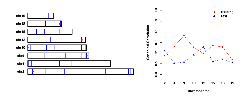
Figure 2: Left: Visualization of the genomic coordinates of detected methylation probes. Genes that represented by more than one probes are highlighted by square symbols. Right: Canonical correlations of disease associated genes and methylation probes on eight chromosomes in the training set and the test set.

Table 3: Sparse CCA results for methylation sites and gene expression that are associated with disease free status for TCGA breast cancer data. In the analysis, methylation and gene expression data are assumed to have sparse precision matrix structure. Sparse CCA were performed on the same set of genes with methylation probes on different chromosomes. Chromosomes with canonical correlation greater than 0.5 on both the training and test set are listed with the number of probes associated with disease free status and the probes form the support of canonical directions.

Number of Genes Chromosome probes Methylation probes RRM2, ILF2, ORC6L, SUSD3, SHCBP1 2 269 cg04799980, cg08022717, cg10142874, cg13052887, cg16297938, cg24011073, cg26364080, cg27060355 SLC26A9, C15orf52, NPM2, DNAH11, RAB6B, LIN28, STC2 4 143 cg04812351, cg14505741, cg15566751, cg15763121, cg17232991 RGS6, ORC6L, PTPRH, GPX2, QSOX2, NPM2, SCG3, RAB6B, L1CAM, STC2, REG1A 9 89 cg01729066, cg02127980, cg03693099, cg13413384, cg13486627, cg13847987, cg14004457, cg14443041, cg21123355 RRM2, SLC26A9, ORC6L, PTPRH, DNAH11, SCG3, LIN28, UMODL1, C11orf9 10 116 cg00827318, cg01162610, cg01520297, cg03182620, cg14522790, cg14999931, cg19302462 QSOX2, SCG3 12 175 cg00417147, cg13074795, cg21881338 C15orf52, NPM2, DNAH11, SELE, RAB6B 15 92 cg11465404, cg18581777, cg21735516 ILF2, SPRR2D, ADCY4, RAB6B, C11orf9, REG1A, SHCBP1 18 37 cg07740306, cg15531009, cg18935516, cg19363889 ORC6L, NPM2, GPR56 19 162 cg06392698, cg06555246

Table 4: Detected methylation probes and their corresponding genes on chromosome 9.

Probe Gene Function $\eta_{i}$ cg01729066 MIR600 microRNA regulating estrogen factors 0.282 cg14004457 MIR455 microRNA regulating estrogen factors 0.347 cg02127980, cg13413384 RXRA retinoic X receptors 0.269, 0.242 cg03693099 CEL fat catalyzation and vitamin absorption 0.286 cg13486627 RG9MTD3 RNA (guanine-9-) methyltransferase -0.479 cg13847987 ABL1 a protein tyrosine kinase functioned in cell differentiation and stress response 0.334 cg21123355 VAV2 a member of the VAV guanine nucleotide exchange factor family of oncogenes 0.312 cg14443041 Intergenic region 0.384

For the purpose of interpretation, the tuning parameters are selected such that a sparse representation of $(\hat{\theta},\hat{\eta})$ is obtained while the canonical correlation is high. More specifically, we require the number of non-zero genes or probes is less than 10 for each chromosome. We split the data into two halves as a test set and a training set. Then we applied the proposed procedure on the training set. To remove false discoveries, we required the canonical correlation on the test set is greater than 0.5. In total, there are eight chromosomes that have methylation probes satisfying the above criteria (shown in Figure 2). In Table 3, we list genes and methylation probes on each chromosome that form the support of detected canonical directions. A further examination of the genomic coordinates of detected methylation probes reveal the physical closeness of some probes. Some detected probes correspond to the same gene. LPIN1 on chromosome 2, RXRA on chromosome 9, DIP2C on chromosome 10, AACS on chromosome 12, and NFATC1 on chromosome 18 are represented by more than one methylation probes (shown in Figure 2). Moreover, 16 of the 25 genes listed in Table 3 are detected more than once as candidate genes associated with methylation probes. ORC6L, RRM2, RAB6B are independently detected from four chromosomes. All these genes have been proposed as prognosis signature for the metastasis of breast cancer (Weigelt et al., 2005; Ma et al., 2003; van’t Veer et al., 2002). Our results suggest the interplay of their expression with detected methylation sites. We list the functional annotation of probes detected on Chromosome 9 in Table 4 .

In this analysis, we assume there is one pair of canonical directions between methylation and gene expression. We note that when the underlying canonical correlation structure is low-rank, the pair of canonical directions obtained from the proposed method lie in the subspace of true canonical directions. The extracted canonical directions can still be used to identify sets of methylate sites that are correlated with gene expression.

7 Proof of Main Theorem

We provide the proof of Theorem 4.1 in this section, which is based on the construction of an oracle sequence. The proof is similar in nature to that in Ma (2013) which focuses on the sparse PCA setting. Specifically, we are going to first define the strong signal sets, and then define an oracle sequence $(\alpha^{(k),ora},\beta^{(k),ora})$ produced by Algorithms 1 and 2 only operating on the strong signal sets. We then show the desired rate of convergence for this oracle sequence. In the end, a probabilistic argument shows that with the help of thresholding, the oracle sequence is identical to the data-driven sequence with high probability. In the following proof, we condition on the second half of the data $(X_{n+1},Y_{n+1}),...,(X_{2n},Y_{2n})$ and the event $\{||\hat{\Omega}_{1}\Sigma_{1}-I||\vee||\hat{\Omega}_{2}\Sigma_{2}-I||=o(1)\}$. The “with probability” argument is understood to be with conditional probability unless otherwise specified. We keep using the notations $p=p_{1}\vee p_{2}$ and $s=s_{1}\vee s_{2}$.

7.1 Construction of the Oracle Sequence

We first define the strong signal set by

$$H_{1}=\left\{k:|\alpha_{k}|\geq\delta_{1}\sqrt{\frac{\log p_{1}}{n}}\right\},\quad H_{2}=\left\{k:|\beta_{k}|\geq\delta_{2}\sqrt{\frac{\log p_{2}}{n}}\right\}.$$ (14)

We denote their complement in $\{1,2,...,p_{1}\}$ and $\{1,2,...,p_{2}\}$ by $L_{1}$ and $L_{2}$ respectively. Then we define the oracle version of $\hat{A}$ by taking those coordinates with strong signals. That is,

$$\hat{A}^{ora}=\begin{pmatrix}\hat{A}_{H_{1}H_{2}}&0\\ 0&0\end{pmatrix}.$$

We construct the oracle initializer $(\alpha^{(0),ora},\beta^{(0),ora})$ based on an oracle version of Algorithm 2 with the sets $B_{1}$ and $B_{2}$ replaced by $B_{1}^{ora}=B_{1}\cap H_{1}$ and $B_{2}^{ora}=B_{2}\cap H_{2}$. It is clear that $\alpha^{(0),ora}_{L_{1}}=0$ and $\beta^{(0),ora}_{L_{2}}=0$. Feeding the oracle initializer $(\alpha^{(0),ora},\beta^{(0),ora})$ and the matrix $\hat{A}^{ora}$ into Algorithm 1, we get the oracle sequence $(\alpha^{(k),ora},\beta^{(k),ora})$.

7.2 Data-Driven Thresholding

Algorithms 1 and 2 contain thresholding levels $\gamma_{1}$, $\gamma_{2}$ and $t_{ij}$. These tuning parameters can be specified by users. However, our theory is based on fully data-driven tuning parameters depending on the matrix $\hat{\Omega}_{1}=(\hat{\omega}_{1,ij})$ and $\hat{\Omega}_{2}=(\hat{\omega}_{2,ij})$. In particular, we use

$$t_{ij}=\frac{20\sqrt{2}}{9}\left(\sqrt{||\hat{\Omega}_{1}||\hat{\omega}_{2,jj}}+\sqrt{||\hat{\Omega}_{2}||\hat{\omega}_{1,ii}}+\sqrt{\hat{\omega}_{1,ii}\hat{\omega}_{2,jj}}+\sqrt{8||\hat{\Omega}_{1}||||\hat{\Omega}_{2}||/3}\right),$$

and

$$\gamma_{1}=\Big{(}0.17\min_{i,j}t_{ij}||\hat{\Omega}_{2}||^{1/2}+2.1||\hat{\Omega}_{2}||^{1/2}||\hat{\Omega}_{1}||^{1/2}+7.5||\hat{\Omega}_{2}||\Big{)}\sqrt{\frac{\log p}{n}},$$

$$\gamma_{2}=\Big{(}0.17\min_{i,j}t_{ij}||\hat{\Omega}_{1}||^{1/2}+2.1||\hat{\Omega}_{1}||^{1/2}||\hat{\Omega}_{2}||^{1/2}+7.5||\hat{\Omega}_{1}||\Big{)}\sqrt{\frac{\log p}{n}}.$$

The constants $(\delta_{1},\delta_{2})$ in (14) are set as $\delta_{1}=\delta_{2}=0.08w^{1/2}\min_{i,j}t_{ij}.$ Such choice of thresholding levels are used in both the estimating sequence $(\alpha^{(k)},\beta^{(k)})$ and the oracle sequence $(\alpha^{(k),ora},\beta^{(k),ora})$.

7.3 Outline of Proof

The proof of Theorem 4.1 can be divided into the following three steps.

1. Show that $\hat{A}^{ora}$ is a good approximation of $A=\lambda\alpha\beta^{T}$ in the sense that their first pairs of singular vectors are close. Namely, let $(\hat{\alpha}^{ora},\hat{\beta}^{ora})$ be the first pair of singular vectors of $\hat{A}^{ora}$. We are going to bound $L(\hat{\alpha}^{ora},\alpha)$ and $L(\hat{\beta}^{ora},\beta)$.

2. Show that the oracle sequence $(\alpha^{(k),ora},\beta^{(k),ora})$ converges to $(\hat{\alpha}^{ora},\hat{\beta}^{ora})$ after finite steps of iterations.

3. Show that the estimating sequence $(\alpha^{(k)},\beta^{(k)})$ and the oracle sequence $(\alpha^{(k),ora},\beta^{(k),ora})$ are identical with high probability up to the necessary number of steps for convergence. Here, we need to first show that the oracle initializer $(\alpha^{(0),ora},\beta^{(0),ora})$ is identical to the actual $(\alpha^{(0)},\beta^{(0)})$. Then we are going to show the thresholding step in Algorithm 1 kills all the small coordinates so that the oracle sequence is identical to the estimating sequence under iteration.

7.4 Preparatory Lemmas

In this part, we present lemmas corresponding to the three steps in the outline of proof. The first lemma corresponds to Step 1.

Lemma 7.1

Under Assumptions A and B, we have

$$L(\hat{\alpha}^{ora},\alpha)^{2}\vee L(\hat{\beta}^{ora},\beta)^{2}\leq C\Bigg{(}s\Big{(}\frac{\log p}{n}\Big{)}^{1-q/2}+||\theta-\alpha|^{2}|\vee||\eta-\beta||^{2}\Bigg{)},$$

with probability at least $1-O(p^{-2})$ for some constant $C>0$.

Let $(\hat{l}_{1},\hat{l}_{2})$ be the first and second singular values of $\hat{A}^{ora}$. Then we have the following results, corresponding to Step 2.

Lemma 7.2

Under Assumptions A and B, we have

$$L({\alpha}^{(1),ora},\hat{\alpha}^{ora})^{2}\leq 4\left|\frac{\hat{l}_{2}}{\hat{l}_{1}}\right|^{2}+\frac{32\gamma_{1}^{2}|H_{1}|}{|\hat{l}_{1}|^{2}},$$

$$L({\beta}^{(1),ora},\hat{\beta}^{ora})^{2}\leq 4\left|\frac{\hat{l}_{2}}{\hat{l}_{1}}\right|^{2}+\frac{32\gamma_{2}^{2}|H_{2}|}{|\hat{l}_{1}|^{2}},$$

for $k=1$, and

$$L({\alpha}^{(k),ora},\hat{\alpha}^{ora})^{2}\leq\max\Bigg{(}4\left|\frac{\hat{l}_{2}}{\hat{l}_{1}}\right|^{2}\frac{64\gamma_{2}^{2}|H_{2}|}{|\hat{l}_{1}|^{2}}+\frac{64\gamma_{1}^{2}|H_{1}|}{|\hat{l}_{1}|^{2}},\Big{(}32\left|\frac{\hat{l}_{2}}{\hat{l}_{1}}\right|^{4}\Big{)}^{[k/2]}\Bigg{)},$$

$$L({\beta}^{(k),ora},\hat{\beta}^{ora})^{2}\leq\max\Bigg{(}4\left|\frac{\hat{l}_{2}}{\hat{l}_{1}}\right|^{2}\frac{64\gamma_{1}^{2}|H_{1}|}{|\hat{l}_{1}|^{2}}+\frac{64\gamma_{2}^{2}|H_{2}|}{|\hat{l}_{1}|^{2}},\Big{(}32\left|\frac{\hat{l}_{2}}{\hat{l}_{1}}\right|^{4}\Big{)}^{[k/2]}\Bigg{)},$$

for all $k\geq 2$ with probability at least $1-O(p^{-2})$.

The quantities $|\hat{l}_{1}|$, $|\hat{l}_{2}/\hat{l}_{1}|$, $|H_{1}|$ and $|H_{2}|$ are determined by the following lemma.

Lemma 7.3

With probability at least $1-O(p^{-2})$,

$$|\hat{l}_{2}|^{2} \leq C\Bigg{(}s\Big{(}\frac{\log p}{n}\Big{)}^{1-q/2}+||\theta-\alpha||^{2}\vee||\eta-\beta||^{2}\Bigg{)},$$

$$|\hat{l}_{1}|^{-2} \leq C.$$

Moreover,

$$|H_{1}|\leq C\Bigg{(}s_{1}\Big{(}\frac{\log p_{1}}{n}\Big{)}^{-q/2}+\Big{(}\frac{\log p_{1}}{n}\Big{)}^{-1}||\theta-\alpha||^{2}\Bigg{)},$$

$$|H_{2}|\leq C\Bigg{(}s_{2}\Big{(}\frac{\log p_{2}}{n}\Big{)}^{-q/2}+\Big{(}\frac{\log p_{2}}{n}\Big{)}^{-1}||\eta-\beta||^{2}\Bigg{)},$$

for some constant $C>0$.

Finally, we show that the oracle sequence and the actual sequence are identical with high probability, corresponding to Step 3. For the initializer, we have the following lemma.

Lemma 7.4

Under Assumptions A and B, we have $B_{1}^{ora}=B_{1}$ and $B_{2}^{ora}=B_{2}$ with probability at least $1-O(p^{-2})$. Thus, $(\alpha^{(0),ora},\beta^{(0),ora})=(\alpha^{(0)},\beta^{(0)})$.

We proceed to analyze the sequence for $k\geq 1$ using mathematical induction. By iteration in Algorithm 1, we have

$$\alpha^{(k),ora}=\frac{T(\hat{A}^{ora}\beta^{(k-1),ora},\gamma_{1})}{||T(\hat{A}^{ora}\beta^{(k-1),ora},\gamma_{1})||},\quad\beta^{(k),ora}=\frac{T(\hat{A}^{ora,T}\alpha^{(k-1),ora},\gamma_{2})}{||T(\hat{A}^{ora,T}\alpha^{(k-1),ora},\gamma_{2})||}.$$

Suppose we have $(\alpha^{(k-1),ora},\beta^{(k-1),ora})=(\alpha^{(k-1)},\beta^{(k-1)})$. Then as long as

$$T(\hat{A}^{ora}\beta^{(k-1),ora},\gamma_{1}) = T(\hat{A}\beta^{(k-1),ora},\gamma_{1})$$ (15)

$$T(\hat{A}^{ora,T}\alpha^{(k-1),ora},\gamma_{2}) = T(\hat{A}^{T}\alpha^{(k-1),ora},\gamma_{2}),$$ (16)

we have $(\alpha^{(k),ora},\beta^{(k),ora})=(\alpha^{(k)},\beta^{(k)})$. Hence, it is sufficient to prove (15) and (16). Then, the result follows from mathematical induction. Without loss of generality, we analyze (15) as follows. Since $\beta_{L_{2}}^{(0),ora}=0$, we may assume $\beta_{L_{2}}^{(k-1),ora}=0$ at the $k$-th step. The vectors $\hat{A}^{ora}\beta^{(k-1),ora}$ and $\hat{A}\beta^{(k-1),ora}$ are respectively

$$\hat{A}^{ora}\beta^{(k-1),ora}=\begin{pmatrix}\hat{A}_{H_{1}H_{2}}&0\\ 0&0\end{pmatrix}\begin{pmatrix}\beta^{(k-1),ora}_{H_{2}}\\ 0\end{pmatrix}=\begin{pmatrix}\hat{A}_{H_{1}H_{2}}\beta^{(k-1),ora}_{H_{2}}\\ 0\end{pmatrix},$$

$$\hat{A}\beta^{(k-1),ora}=\begin{pmatrix}\hat{A}_{H_{1}H_{2}}&\hat{A}_{H_{1}L_{2}}\\ \hat{A}_{L_{1}H_{2}}&\hat{A}_{L_{1}L_{2}}\end{pmatrix}\begin{pmatrix}\beta^{(k-1),ora}_{H_{2}}\\ 0\end{pmatrix}=\begin{pmatrix}\hat{A}_{H_{1}H_{2}}\beta^{(k-1),ora}_{H_{2}}\\ \hat{A}_{L_{1}H_{2}}\beta_{H_{2}}^{(k-1),ora}\end{pmatrix}.$$

Hence, as long as $||\hat{A}_{L_{1}H_{2}}\beta_{H_{2}}^{(k-1),ora}||_{\infty}\leq\gamma_{1}$, (15) holds. Similarly, as long as $||\hat{A}_{H_{1}L_{2}}^{T}\alpha_{H_{1}}^{(k-1),ora}||_{\infty}\leq\gamma_{2}$, (16) holds. This is guaranteed by the following lemma.

Lemma 7.5

For any sequence of unit vectors $(a^{(k)},b^{(k)})\in\mathbb{R}^{\left|H_{1}\right|}\times\mathbb{R}^{\left|H_{2}\right|}$, with $k=1,2,...,K$ for some $K=O(1)$. We assume that they only depend on $\hat{A}_{H_{1}H_{2}}$. Then, under the current choice of $(\gamma_{1},\gamma_{2})$, we have

$$||\hat{A}_{L_{1}H_{2}}b^{(k)}||_{\infty}\leq\gamma_{1},\quad||\hat{A}_{H_{1}L_{2}}^{T}a^{(k)}||_{\infty}\leq\gamma_{2},$$

for all $k=1,...,K$ with probability at least $1-O(p^{-2})$.

7.5 Proof of Theorem 4.1

Proof 7.1 (Proof of Theorem 4.1).

In the following proof, $C$ denotes a generic constant which may vary from line to line. Without loss of generality, we prove convergence of $\alpha^{(k)}$. By Lemma 7.4 and Lemma 7.5, $\alpha^{(k)}=\alpha^{(k),ora}$ for all $k=1,2,...,K$ with probability $1-O(p^{-2})$. Hence, it is sufficient to prove convergence of $\alpha^{(k),ora}$. Lemma 7.2 implies that for $k=2,3,...,K$,

$$L(\alpha^{(k),ora},\hat{\alpha}^{ora})^{2} \leq \max\Bigg{(}4\left|\frac{\hat{l}_{2}}{\hat{l}_{1}}\right|^{2}\frac{64\gamma_{2}^{2}|H_{2}|}{|\hat{l}_{1}|^{2}}+\frac{64\gamma_{1}^{2}|H_{1}|}{|\hat{l}_{1}|^{2}},\Big{(}32\left|\frac{\hat{l}_{2}}{\hat{l}_{1}}\right|^{4}\Big{)}^{[k/2]}\Bigg{)}$$

$$\leq \max\Bigg{(}4\left|\frac{\hat{l}_{2}}{\hat{l}_{1}}\right|^{2}\frac{64\gamma_{2}^{2}|H_{2}|}{|\hat{l}_{1}|^{2}}+\frac{64\gamma_{1}^{2}|H_{1}|}{|\hat{l}_{1}|^{2}},32\left|\frac{\hat{l}_{2}}{\hat{l}_{1}}\right|^{4}\Bigg{)}$$

According to Lemma 7.3, we have

$$32\left|\frac{\hat{l}_{2}}{\hat{l}_{1}}\right|^{4}\leq C\Bigg{(}s\Big{(}\frac{\log p}{n}\Big{)}^{1-q/2}+||\theta-\alpha||^{2}\vee||\beta-\eta||^{2}\Bigg{)}^{2}.$$

We also have

$$4\left|\frac{\hat{l}_{2}}{\hat{l}_{1}}\right|^{2}\frac{64\gamma_{2}^{2}|H_{2}|}{|\hat{l}_{1}|^{2}}+\frac{64\gamma_{1}^{2}|H_{1}|}{|\hat{l}_{1}|^{2}}$$

$$\leq C\Big{(}\gamma_{2}^{2}|H_{2}|+\gamma_{1}^{2}|H_{1}|\Big{)}$$

$$\leq C\frac{\log p}{n}\Bigg{(}s\Big{(}\frac{\log p}{n}\Big{)}^{-q/2}+\Big{(}\frac{\log p}{n}\Big{)}^{-1}||\theta-\alpha||^{2}\Bigg{)}$$

$$\leq C\Bigg{(}s\Big{(}\frac{\log p}{n}\Big{)}^{1-q/2}+||\theta-\alpha||^{2}\Bigg{)}.$$

Hence, the desired bound holds for $k=2,3,...,K$. For $k=1$, by Lemma 7.2, we have

$$L({\alpha}^{(1),ora},\hat{\alpha}^{ora})^{2}\leq 4\left|\frac{\hat{l}_{2}}{\hat{l}_{1}}\right|^{2}+\frac{32\gamma_{1}^{2}|H_{1}|}{|\hat{l}_{1}|^{2}}\leq C\Bigg{(}s\Big{(}\frac{\log p}{n}\Big{)}^{1-q/2}+||\theta-\alpha||^{2}\Bigg{)}.$$

Therefore, we have proved the bound of $L(\alpha^{(k),ora},\alpha^{ora})^{2}$ for all $k=1,2,...,K$. Combining this result and Lemma 7.1, we have

$$L({\alpha}^{(k),ora},{\alpha})^{2}\leq C\Bigg{(}s\Big{(}\frac{\log p}{n}\Big{)}^{1-q/2}+||\theta-\alpha||^{2}\vee||\beta-\eta||^{2}\Bigg{)},$$

for $k=1,2,...,K$. The final bound follows from the triangle inequality applied to the equation above and the fact that

$$L(\alpha,\theta)\leq C\Big{(}||\alpha-\theta||\wedge||\alpha+\theta||\Big{)}\leq C||\alpha-\theta||.$$

The same analysis applies for $L({\beta}^{(k),ora},{\eta})^{2}$. Thus, the result is obtained conditioning on

$$(X_{n+1},Y_{n+1}),...,(X_{2n},Y_{2n}).$$

Since we assume $\xi_{\Omega}=o(1)$ with probability at least $1-O(p^{-2})$, the unconditional result also holds.

Appendix

Appendix A Technical Lemmas

We define the high-signal and low-signal set of $(\theta,\eta)$ by

$$H^{\prime}_{1}=\left\{k:|\theta_{k}|\geq\frac{1}{2}\delta_{1}\sqrt{\frac{\log p_{1}}{n}}\right\},\quad H^{\prime}_{2}=\left\{k:|\eta_{k}|\geq\frac{1}{2}\delta_{2}\sqrt{\frac{\log p_{2}}{n}}\right\},$$

and $L_{1}^{\prime}=\{1,...,p_{1}\}-H_{1}^{\prime}$ and $L_{2}^{\prime}=\{1,...,p_{2}\}-H_{2}^{\prime}$.

Lemma A.1.

We have

$$|H^{\prime}_{1}|\leq(\delta_{1}/2)^{-q}s_{1}\Bigg{(}\frac{\log p_{1}}{n}\Bigg{)}^{-q/2},\quad|H^{\prime}_{2}|\leq(\delta_{2}/2)^{-q}s_{2}\Bigg{(}\frac{\log p_{2}}{n}\Bigg{)}^{-q/2},$$

$$|H_{1}|\leq(\delta_{1}/2)^{-q}s_{1}\Bigg{(}\frac{\log p_{1}}{n}\Bigg{)}^{-q/2}+(\delta_{1}/2)^{-2}\Bigg{(}\frac{\log p_{1}}{n}\Bigg{)}^{-1}||\theta-\alpha||^{2},$$

$$|H_{2}|\leq(\delta_{2}/2)^{-q}s_{2}\Bigg{(}\frac{\log p_{2}}{n}\Bigg{)}^{-q/2}+(\delta_{2}/2)^{-2}\Bigg{(}\frac{\log p_{2}}{n}\Bigg{)}^{-1}||\eta-\beta||^{2},$$

$$|L_{1}-L_{1}^{\prime}|=|H^{\prime}_{1}-H_{1}|\leq 2(\delta_{1}/2)^{-q}s_{1}\Bigg{(}\frac{\log p_{1}}{n}\Bigg{)}^{-q/2}+(\delta_{1}/2)^{-2}\Bigg{(}\frac{\log p_{1}}{n}\Bigg{)}^{-1}||\theta-\alpha||^{2},$$

$$|L_{2}-L_{2}^{\prime}|=|H^{\prime}_{2}-H_{2}|\leq 2(\delta_{2}/2)^{-q}s_{2}\Bigg{(}\frac{\log p_{2}}{n}\Bigg{)}^{-q/2}+(\delta_{2}/2)^{-2}\Bigg{(}\frac{\log p_{2}}{n}\Bigg{)}^{-1}||\eta-\beta||^{2}.$$

For the transformed data $\{(\tilde{X}_{i},\tilde{Y}_{i})\}_{i=1}^{n}$, it has a latent variable representation

$$\tilde{X}_{i}=\sqrt{\lambda}\alpha Z_{i}+X_{i}^{\prime},\quad\tilde{Y}_{i}=\sqrt{\lambda}\beta Z_{i}+Y_{i}^{\prime},$$

where $Z_{i},X_{i}^{\prime},Y_{i}^{\prime}$ are independent, $Z_{i}\sim N(0,1)$ and $X_{i}^{\prime}$ and $Y_{i}^{\prime}$ are Gaussian vectors.

Lemma A.2.

The latent representation above exists in the sense that $\mbox{\rm Cov}(X^{\prime})\geq 0$ and $\mbox{\rm Cov}(Y^{\prime})\geq 0$. Moreover, we have

$$||\mbox{\rm Cov}(X^{\prime})||\leq\big{(}1+o(1)\big{)}||\hat{\Omega}_{1}||,\quad\mbox{\rm and}\quad||\mbox{\rm Cov}(Y^{\prime})||\leq\big{(}1+o(1)\big{)}||\hat{\Omega}_{2}||.$$

Lemma A.3 (Johnstone (2001)).

Given $Z_{1},...,Z_{n}$ i.i.d. $N(0,1)$. For each $t\in(0,1/2)$,

$$\mathbb{P}\Bigg{(}\left|\frac{1}{n}\sum_{i=1}^{n}Z_{i}^{2}-1\right|>t\Bigg{)}\leq 2\exp\Big{(}-\frac{3nt^{2}}{16}\Big{)}.$$

Lemma A.4.

Let $X_{H_{1}}^{\prime}$ be an $n\times|H_{1}|$ matrix with $X_{i,H_{1}}^{\prime}$ being the $i$-th row and $Y_{H_{2}}^{\prime}$ be an $n\times|H_{2}|$ matrix with $Y_{i,H_{2}}^{\prime}$ being the $i$-th row. We have for any $t>0$,

$$\mathbb{P}\Bigg{(}||X_{H_{1}}^{\prime T}X_{H_{1}}^{\prime}||>1.01||{\hat{\Omega}}_{1}||\Big{(}n+2\big{(}\sqrt{n|H_{1}|}+nt\big{)}+\big{(}\sqrt{|H_{1}|}+\sqrt{n}t\big{)}^{2}\Big{)}\Bigg{)}\leq 2e^{-nt^{2}/2},$$

$$\mathbb{P}\Bigg{(}||Y_{H_{2}}^{\prime T}Y_{H_{2}}^{\prime}||>1.01||{\hat{\Omega}}_{2}||\Big{(}n+2\big{(}\sqrt{n|H_{2}|}+nt\big{)}+\big{(}\sqrt{|H_{2}|}+\sqrt{n}t\big{)}^{2}\Big{)}\Bigg{)}\leq 2e^{-nt^{2}/2},$$

$$\mathbb{P}\Bigg{(}||X_{H_{1}}^{\prime T}Y_{H_{2}}^{\prime}||>1.03||\hat{\Omega}_{1}||^{1/2}||\hat{\Omega}_{2}||^{1/2}\Big{(}\sqrt{|H_{1}|n}+\sqrt{|H_{2}|n}+t\sqrt{n}\Big{)}\Bigg{)}\leq\big{(}|H_{1}|\wedge|H_{2}|\big{)}e^{-3n/64}+e^{-t^{2}/2}.$$

Lemma A.5.

We have for any $t>0$,

$$\mathbb{P}\Bigg{(}\left\|\sum_{i=1}^{n}Z_{i}X_{i,H_{1}}^{\prime}\right\|>1.03||\hat{\Omega}_{1}||^{1/2}\Big{(}(t+1)\sqrt{n}+\sqrt{|H_{1}|n}\Big{)}\Bigg{)}\leq e^{-3n/64}+e^{-t^{2}/2},$$

$$\mathbb{P}\Bigg{(}\left\|\sum_{i=1}^{n}Z_{i}Y_{i,H_{2}}^{\prime}\right\|>1.03||\hat{\Omega}_{2}||^{1/2}\Big{(}(t+1)\sqrt{n}+\sqrt{|H_{2}|n}\Big{)}\Bigg{)}\leq e^{-3n/64}+e^{-t^{2}/2},$$

$$\mathbb{P}\Bigg{(}\left\|\sum_{i=1}^{n}Z_{i}X_{i,L_{1}}^{\prime}\right\|_{\infty}>1.03||\hat{\Omega}_{1}||^{1/2}(t+2)\sqrt{n}\Bigg{)}\leq|L_{1}|\Big{(}e^{-3n/64}+e^{-t^{2}/2}\Big{)},$$

$$\mathbb{P}\Bigg{(}\left\|\sum_{i=1}^{n}Z_{i}Y_{i,L_{2}}^{\prime}\right\|_{\infty}>1.03||\hat{\Omega}_{2}||^{1/2}(t+2)\sqrt{n}\Bigg{)}\leq|L_{2}|\Big{(}e^{-3n/64}+e^{-t^{2}/2}\Big{)}.$$

Lemma A.6.

We have

$$||\hat{A}_{H_{1}H_{2}}-A_{H_{1}H_{2}}|| \leq C\Bigg{(}s^{1/2}\Bigg{(}\frac{\log p}{n}\Bigg{)}^{1/2-q/4}+||\alpha-\theta||\vee||\beta-\eta||\Bigg{)},$$

$$\max_{i=1,2}|\hat{l}_{i}-{l}_{i}| \leq C\Bigg{(}s^{1/2}\Bigg{(}\frac{\log p}{n}\Bigg{)}^{1/2-q/4}+||\alpha-\theta||\vee||\beta-\eta||\Bigg{)},$$

$$l_{1} \geq C^{-1},$$

$$l_{2} = 0$$

for some constant $C>0$ with probability at least $1-O(p^{-2})$. The quantities $\hat{l}_{i}$ and $l_{i}$ are the $i$-th singular values of $\hat{A}_{H_{1}H_{2}}$ and $A_{H_{1}H_{2}}$ respectively.

Appendix B Analysis of the Initializer

We show that the Algorithm 2 actually returns a consistent estimator of leading pair of singular vectors $\left(\alpha^{(0)},\beta^{(0)}\right)$, which serves as a good candidate for the power method in Algorithm 1. To be specific, with high probability, the initialization procedure correctly kills all low signal coordinates to zeros, i.e. $\alpha_{L_{1}}^{(0)}=0$ and $\beta_{L_{2}}^{(0)}=0$, by the thresholding step. On the other hand, although Algorithm 2 cannot always correctly pick all strong signal coordinates, it does pick those much stronger ones such that $\left(\alpha^{(0)},\beta^{(0)}\right)$ is still consistent up to a sign. The properties are summarized below.

Lemma B.1.

With probability $1-Cp^{-2}$, we have that,

1. $B_{i}\subset H_{i}$, $i=1,2$;

2. $\left|\hat{l}_{i}-\hat{l}_{i}^{B}\right|\rightarrow 0$ for $i=1,2.$ where $\hat{l}_{i}$ and $\hat{l}_{i}^{B}$ are the $i$th singular value of $\hat{A}_{H_{1}H_{2}}$ and $\hat{A}_{B_{1}B_{2}}$;

3. $\alpha^{(0)}$ and $\beta^{(0)}$ are consistent, i.e., $L\left(\alpha^{(0)},\hat{\alpha}^{ora}\right)\rightarrow 0$ and $L\left(\beta^{(0)},\hat{\beta}^{ora}\right)\rightarrow 0$.

The procedure is to select those strong signal coordinates of $\alpha$ and $\beta$ and is similar to the “diagonal thresholding” sparse PCA method proposed by Johnstone and Lu (2009). However, unlike the PCA setting, we cannot get the information of each coordinate through its corresponding diagonal entry of the sample covariance matrix. Instead, we measure the strength of coordinates in terms of the maximum entry among its corresponding row or column of the sample covariance matrix and still can capture all coordinates of $\alpha$ and $\beta$ above the level of $\left(\frac{\log p}{n}\right)^{1/4}$. The sparsity assumption in Equation (10) is needed to guarantee the consistency of the initial estimator $\left(\alpha^{(0)},\beta^{(0)}\right)$.

The proof is developed in the following. In the first part, we prove the three results in Lemma B.1 along with stating some useful propositions. We then prove those propositions in the second part.

B.1 Proof of Lemma B.1

Proof B.2 (Proof of Result 1).

We start with showing the first result $B_{i}\subset H_{i}$. In fact we show that the index set $B_{i}$screens out all weak signal coordinates as well as captures all coordinates with much stronger signal coordinates $\sqrt{\frac{\log p}{n}}s^{\frac{1}{2-q}}$, compared with the thresholding $\sqrt{\frac{\log p}{n}}$of $H_{i}$. By the sparsity assumption (10), clearly $B_{i}$also captures all coordinates with much stronger signal $\left(\frac{\log p}{n}\right)^{1/4}$. To be specific, we show that with probability $1-Cp^{-2}$, we have

$$B_{i}^{-}\subset B_{i}\subset H_{i},$$ (17)

where the index set of those stronger signal coordinates are defined as follows,

$$B_{1}^{-}=\left\{i,\left|\alpha_{i}\right|>\phi\sqrt{\frac{\log p}{n}}s_{2}^{\frac{1}{2-q}}\right\},B_{2}^{-}=\left\{i,\left|\beta_{i}\right|>\phi\sqrt{\frac{\log p}{n}}s_{1}^{\frac{1}{2-q}}\right\}.$$

The constant $\phi$ is determined in the analysis. $\phi=2\max_{i,j}t_{ij}C_{\lambda}^{-1}\left(\frac{\sqrt{W}}{0.6}\left(2W^{1/2}\right)^{\frac{-q}{2-q}}\right)^{1/2}$.

Recall that $\hat{A}=\frac{1}{n}\sum_{i}\tilde{X}_{i}\tilde{Y}_{i}^{T}$ with conditional mean $\mathbb{E}\hat{A}=A=\lambda\alpha\beta^{T}=\left(a_{ij}\right)_{p_{1}\times p_{2}}$. The result (17) can be shown in two steps. During the first step we show that with probability $1-Cp^{-2}$, the index set $B_{i}$ satisfies $B_{i}^{--}\subset B_{i}\subset B_{i}^{++}$, where for simplicity we pick $\kappa_{-}=0.09,\kappa_{+}=2$ and

$$B_{1}^{++}=\left\{i:\max_{j}\frac{|{a}_{ij}|}{t_{ij}}>\kappa_{-}\sqrt{\frac{1}{n}\log p}\right\},B_{1}^{--}=\left\{i:\max_{j}\frac{|{a}_{ij}|}{t_{ij}}>\kappa_{+}\sqrt{\frac{1}{n}\log p}\right\},$$

$$B_{2}^{++}=\left\{j:\max_{i}\frac{|{a}_{ij}|}{t_{ij}}>\kappa_{-}\sqrt{\frac{1}{n}\log p}\right\},B_{2}^{--}=\left\{j:\max_{i}\frac{|{a}_{ij}|}{t_{ij}}>\kappa_{+}\sqrt{\frac{1}{n}\log p}\right\}.$$

For the second step, we show that $B_{i}^{++}\subset H_{i}$ and $B_{i}^{--}\subset B_{i}^{-}$ with probability $1-Cp^{-2}$. We present these two results in the following two propositions.

Proposition B.3.

With probability $1-Cp^{-2}$, we have $B_{i}^{--}\subset B_{i}\subset B_{i}^{++}$ for $i=1,2.$

Proposition B.4.

With probability $1-Cp^{-2}$, we have $B_{i}^{++}\subset H_{i}$ and $B_{i}^{--}\subset B_{i}^{-}$ for $i=1,2.$

Thus, the proof is complete.

Before proving Result 2 and Result 3, we need the following proposition.

Proposition B.5.

Define

$$e_{B}^{2}=\max\left\{\sum_{i\in\left(B_{1}^{-}\right)^{c}}\alpha_{i}^{2},\sum_{i\in\left(B_{2}^{-}\right)^{c}}\beta_{i}^{2}\right\}\mbox{\rm.}$$ (18)

Then we have for some constants $C_{1},C_{2}>0$,

$$e_{B}^{2}\leq C_{1}\left(\frac{\log p}{n}\right)^{1-q/2}\left(s_{1}^{2}\vee s_{2}^{2}\right)+C_{2}\xi_{\Omega}^{2}.$$ (19)

Moreover, under our assumptions (10) and (11), we obtain $e_{B}=o(1)$ with probability $1-Cp^{-2}$.

Now we restrict our attention on the event on which the result (17) holds, which is valid with high probability $1-Cp^{-2}$. Define index set $D_{i}=H_{i}\backslash B_{i}$ and

$$\hat{A}_{H_{1}H_{2}}^{B_{1}B_{2}}=\left(\begin{array}[]{cc}\hat{A}_{B_{1}B_{2}}&0\\ 0&0\end{array}\right)_{\left|H_{1}\right|\times\left|H_{2}\right|}.$$

Proof B.6 (Proof of Result 2).

We show the second result $\left|\hat{l}_{i}-\hat{l}_{i}^{B}\right|\rightarrow 0$ for $i=1,2.$ Note that $\hat{l}_{i}^{B}$ is the $i$th singular value of $\hat{A}_{B_{1}B_{2}}$ and hence is also the $i$th singular value of $\hat{A}_{H_{1}H_{2}}^{B_{1}B_{2}}$. Applying Weyl’s theorem, we obtain that

$$\left|\hat{l}_{i}-\hat{l}_{i}^{B}\right|\leq\left\|\hat{A}_{H_{1}H_{2}}-\hat{A}_{H_{1}H_{2}}^{B_{1}B_{2}}\right\|\leq\left\|\hat{A}_{D_{1}B_{2}}\right\|+\left\|\hat{A}_{B_{1}D_{2}}\right\|+\left\|\hat{A}_{D_{1}D_{2}}\right\|.$$ (20)

To bound $\left\|\hat{A}_{D_{1}B_{2}}\right\|,$ we apply the latent variable representation in Lemma A.2 and obtain that $\hat{A}_{D_{1}B_{2}}=\sum_{j=1}^{4}G_{j}$, where

$$G_{1}=\frac{\lambda Z^{T}Z}{n}\alpha_{D_{1}}\beta_{B_{2}}^{T},\mbox{\rm}G_{2}=\frac{1}{n}X_{D_{1}}^{\prime T}Y_{B_{2}}^{\prime},\mbox{\rm}G_{3}=\frac{\sqrt{\lambda}\alpha_{D_{1}}Z^{T}Y_{B_{2}}^{\prime}}{n},\mbox{\rm}G_{4}=\frac{\sqrt{\lambda}X_{D_{1}}^{\prime T}Z\beta_{B_{2}}^{T}}{n}.$$

Now we bound $G_{j}$ separately as follows. According to Lemma A.3, Proposition B.5 and the fact $\left\|\beta_{B_{2}}\right\|\leq\left\|\beta\right\|\leq\left\|\hat{\Omega}_{2}\Sigma_{2}\right\|\left\|\eta\right\|=\left(1+o(1)\right)\left\|\eta\right\|$, we obtain that with probability $1-Cp^{-2}$

$$\left\|G_{1}\right\| \leq \lambda\left(1+O(\sqrt{\frac{\log p}{n}})\right)\left\|\alpha_{D_{1}}\right\|\left\|\beta_{B_{2}}\right\|\leq\left(1+o(1)\right)\lambda\left\|\eta\right\|\left\|\alpha_{\left(B_{1}^{-}\right)^{c}}\right\|$$

$$\leq \left(1+o(1)\right)\lambda\left\|\theta\right\|e_{B},$$

where the second inequality follows from $D_{1}\subset\left(B_{1}^{-}\right)^{c}$. The third inequality in Lemma A.4 implies that with probability $1-Cp^{-2},$

$$\left\|G_{2}\right\|\leq\left(C(\sqrt{\frac{\log p}{n}}+\sqrt{\frac{\left|H_{1}\right|}{n}}+\sqrt{\frac{\left|H_{2}\right|}{n}})\right)=o(e_{B}),$$

where the last inequality is due to Lemma A.1 $\left|H_{i}\right|=O\left(s_{i}\left(\frac{\log p}{n}\right)^{-q/2}\right)$ and Proposition B.5. Moreover, the first two inequalities in Lemma A.5 further imply that with probability $1-Cp^{-2},$

$$\left\|G_{3}\right\| \leq \left(C(\sqrt{\frac{\log p}{n}}+\sqrt{\frac{\left|H_{2}\right|}{n}})\left\|\alpha_{D_{1}}\right\|\right)\leq o(\left\|\alpha_{\left(B_{1}^{-}\right)^{c}}\right\|)=o(e_{B}),$$

$$\left\|G_{4}\right\| \leq \left(C(\sqrt{\frac{\log p}{n}}+\sqrt{\frac{\left|H_{1}\right|}{n}})\left\|\beta_{B_{2}}\right\|\right)=o(e_{B}).$$

Combining the above four results, we obtain that $\left\|\hat{A}_{D_{1}B_{2}}\right\|\leq\left(1+o(1)\right)\lambda\left\|\theta\right\|e_{B}$ with probability $1-Cp^{-2}$. Similarly we can obtain that $\left\|\hat{A}_{B_{1}D_{2}}\right\|\leq\left(1+o(1)\right)\lambda\left\|\theta\right\|e_{B}$ with probability $1-Cp^{-2}$. To bound $\left\|\hat{A}_{D_{1}D_{2}}\right\|$, similarly we can write $\hat{A}_{D_{1}B_{2}}=\sum_{j=1}^{4}F_{j}$, where

$$F_{1}=\frac{\lambda Z^{T}Z}{n}\alpha_{D_{1}}\beta_{D_{2}}^{T},\mbox{\rm}F_{2}=\frac{1}{n}X_{D_{1}}^{\prime T}Y_{D_{2}}^{\prime},\mbox{\rm}F_{3}=\frac{\sqrt{\lambda}\alpha_{D_{1}}Z^{T}Y_{D_{2}}^{\prime}}{n},\mbox{\rm}F_{4}=\frac{\sqrt{\lambda}X_{D_{1}}^{\prime T}Z\beta_{D_{2}}^{T}}{n}.$$

Note that $D_{i}\subset\left(B_{i}^{-}\right)^{c}$ for $i=1,2$. Lemma A.4, Lemma A.5 and Proposition B.5 imply that with probability $1-Cp^{-2}$,

$$\left\|F_{1}\right\| \leq \lambda\left(1+O(\sqrt{\frac{\log p}{n}})\right)\left\|\alpha_{D_{1}}\right\|\left\|\beta_{D_{2}}\right\|\leq C\left\|\alpha_{\left(B_{1}^{-}\right)^{c}}\right\|\left\|\beta_{\left(B_{2}^{-}\right)^{c}}\right\|=o(e_{B}),$$

$$\left\|F_{2}\right\| \leq \left(C(\sqrt{\frac{\log p}{n}}+\sqrt{\frac{\left|H_{1}\right|}{n}}+\sqrt{\frac{\left|H_{2}\right|}{n}})\right)=o(e_{B}),$$

$$\left\|F_{3}\right\| \leq o(\left\|\alpha_{\left(B_{1}^{-}\right)^{c}}\right\|)=o(e_{B}),\left\|F_{4}\right\|\leq o(\left\|\beta_{\left(B_{2}^{-}\right)^{c}}\right\|)=o(e_{B}).$$

Hence we obtain $\left\|\hat{A}_{D_{1}D_{2}}\right\|=o(e_{B}).$ These upper bounds for $\left\|\hat{A}_{D_{1}D_{2}}\right\|,$ $\left\|\hat{A}_{D_{1}D_{2}}\right\|$ and $\left\|\hat{A}_{D_{1}D_{2}}\right\|$, together with Equation (20) imply that with probability $1-Cp^{-2}$,

$$\left|\hat{l}_{i}-\hat{l}_{i}^{B}\right|\leq\left\|\hat{A}_{H_{1}H_{2}}-\hat{A}_{H_{1}H_{2}}^{B_{1}B_{2}}\right\|\leq\left(1+o(1)\right)\left(\left\|\theta\right\|+\left\|\eta\right\|\right)\lambda e_{B}=o(1),$$ (21)

where the last inequality follows from Proposition B.5 and Assumption B ($\max\left\{\left\|\theta\right\|,\left\|\eta\right\|\right\}\leq w^{-1/2}$).

Proof B.7 (Proof of Result 3).

We show that last result $L\left(\alpha^{(0)},\hat{\alpha}^{ora}\right)\rightarrow 0$ and $L\left(\beta^{(0)},\hat{\beta}^{ora}\right)\rightarrow 0$. Note $\alpha^{(0)}$ and $\hat{\alpha}^{ora}\in\mathbb{R}^{p_{1}}$ but all entries in the index set $H_{1}^{c}$ are zeros. Hence we only need to compare them in $\mathbb{R}^{\left|H_{1}\right|}$. Similarly we calculate $L\left(\beta^{(0)},\hat{\beta}^{ora}\right)$ in space $\mathbb{R}^{\left|H_{2}\right|}$. Constraint on coordinates in $H_{1}\times H_{2}$, $\left(\alpha^{(0)},\beta^{(0)}\right)$ and $\left(\hat{\alpha}^{ora},\hat{\beta}^{ora}\right)$ are leading pair of singular vectors of $\hat{A}_{H_{1}H_{2}}^{B_{1}B_{2}}$ and $\hat{A}_{H_{1}H_{2}}$ respectively. We apply Wedin’s theorem (See Stewart and Sun (1990), Theorem 4.4) to $\hat{A}_{H_{1}H_{2}}$ and $\hat{A}_{H_{1}H_{2}}^{B_{1}B_{2}}$ to obtain that

$$\max\left\{L\left(\alpha^{(0)},\hat{\alpha}^{ora}\right),L\left(\beta^{(0)},\hat{\beta}^{ora}\right)\right\} \leq \sqrt{2}\max\left\{\left\|\frac{\alpha^{(0)}\left(\alpha^{(0)}\right)^{T}}{\left\|\alpha^{(0)}\right\|^{2}}-\frac{\hat{\alpha}^{ora}\left(\hat{\alpha}^{ora}\right)^{T}}{\left\|\hat{\alpha}^{ora}\right\|^{2}}\right\|\right.,$$ (22)

$$\left.\left\|\frac{\beta^{(0)}\left(\beta^{(0)}\right)^{T}}{\left\|\beta^{(0)}\right\|^{2}}-\frac{\hat{\beta}^{ora}\left(\hat{\beta}^{ora}\right)^{T}}{\left\|\hat{\beta}^{ora}\right\|^{2}}\right\|\right\}$$

$$\leq \sqrt{2}\frac{\left\|\hat{A}_{H_{1}H_{2}}^{B_{1}B_{2}}-\hat{A}_{H_{1}H_{2}}\right\|}{\delta\left(\hat{A}_{H_{1}H_{2}}^{B_{1}B_{2}},\hat{A}_{H_{1}H_{2}}\right)},$$

where $\delta\left(\hat{A}_{H_{1}H_{2}}^{B_{1}B_{2}},\hat{A}_{H_{1}H_{2}}\right)=\hat{l}_{1}^{B}-\hat{l}_{2}$. The result of Lemma A.6 implies that $\hat{l}_{2}=o(1)$, and Result $2$ we just showed further implies that $\hat{l}_{1}^{B}=(1+o(1))\hat{l}_{1}=(1+o(1))\lambda\left\|\eta\right\|\left\|\theta\right\|$ with probability $1-Cp^{-2}$. Therefore we obtain that with probability $1-Cp^{-2}$, the value $\delta\left(\hat{A}_{H_{1}H_{2}}^{B_{1}B_{2}},\hat{A}_{H_{1}H_{2}}\right)=(1+o(1))\lambda\left\|\eta\right\|\left\|\theta\right\|$ is bounded below and above by constants according to Assumption B. This fact, together with Equations (21) and (22) completes our proof

$$\max\left\{L\left(\alpha^{(0)},\hat{\alpha}^{ora}\right),L\left(\beta^{(0)},\hat{\beta}^{ora}\right)\right\}=o(1),$$

with probability $1-Cp^{-2}$.

B.2 Proofs of Propositions

Proof B.8 (Proof of Proposition B.3).

We first provide concentration inequality for each $\hat{a}_{ij}=\frac{1}{n}\sum_{k}\tilde{X}_{k,i}\tilde{Y}_{k,j}$. By the latent variable representation, we have $\tilde{X}_{1,i}=\sqrt{\lambda}\alpha_{i}Z_{1}+X_{1,i}^{\prime}$ and $\tilde{Y}_{1,j}=\sqrt{\lambda}\beta_{j}Z_{1}+Y_{1,j}^{\prime}$ where $Z_{1}\sim N(0,1)$, $X_{1,i}^{\prime}\sim N\Big{(}0,\mbox{\rm Var}\left(X_{1,i}^{\prime}\right)\Big{)}$ and $Y_{1,j}^{\prime}\sim N\Big{(}0,\mbox{\rm Var}\left(Y_{1,j}^{\prime}\right)\Big{)}$ are independent. This representation leads to

$$\hat{a}_{ij}=\frac{1}{n}\left(\lambda\alpha_{i}\beta_{j}\sum_{k}Z_{k}^{2}+\sum_{k}X_{k,i}^{\prime}Y_{k,j}^{\prime}+\sqrt{\lambda}\alpha_{i}\sum_{k}Z_{k}Y_{k,j}^{\prime}+\sqrt{\lambda}\beta_{j}\sum_{k}Z_{k}X_{k,i}^{\prime}\right).$$

The consistency assumption Equation (11) in Assumption B implies that $\mbox{\rm Var}\left(X_{1,i}^{\prime}\right)\leq\mbox{\rm Var}\left(\tilde{X}_{1,i}\right)=(1+o(1))\hat{\omega}_{1,ii}=(1+o(1))\omega_{1,ii}$. Applying Lemma A.3, we obtain that

$$\mathbb{P}\left(\left|\frac{\lambda\alpha_{i}\beta_{j}}{n}\sum_{k}Z_{k}^{2}-a_{ij}\right|>\lambda\alpha_{i}\beta_{j}t\right)\leq 2\exp\left(-\frac{3nt^{2}}{16}\right).$$ (23)

Following the line of proof in Lemma A.5 and Proposition D.2 in Ma (2013), for $n$ and $p$ large enough (hence $n^{-1}\log p\rightarrow 0$), we have the following concentration inequalities,

$$\mathbb{P}\left(\left|\frac{1}{n}\sum_{k}X_{k,i}^{\prime}Y_{k,j}^{\prime}\right|>\left(1+o(1)\right)b\sqrt{\hat{\omega}_{1,ii}\hat{\omega}_{2,jj}}\sqrt{\frac{\log p}{n}}\right) \leq 2p^{-b^{2}/2},$$ (24)

$$\mathbb{P}\left(\left|\frac{1}{n}\sqrt{\lambda}\beta_{j}\sum_{k}Z_{k}X_{k,i}^{\prime}\right|>\left(1+o(1)\right)b\sqrt{\lambda}\left|\beta_{j}\right|\sqrt{\hat{\omega}_{1,ii}}\sqrt{\frac{\log p}{n}}\right) \leq 2p^{-b^{2}/2},$$ (25)

$$\mathbb{P}\left(\left|\frac{1}{n}\sqrt{\lambda}\alpha_{i}\sum_{k}Z_{k}Y_{k,j}^{\prime}\right|>\left(1+o(1)\right)b\sqrt{\lambda}\left|\alpha_{i}\right|\sqrt{\hat{\omega}_{2,jj}}\sqrt{\frac{\log p}{n}}\right) \leq 2p^{-b^{2}/2}\mbox{\rm.}$$ (26)

Recall the definition of the adaptive thresholding level $t_{ij},$

$$\begin{array}[]{c}t_{ij}=\frac{20\sqrt{2}}{9}\left(\sqrt{\lambda_{\max}\left(\hat{\Omega}_{1}\right)\hat{\omega}_{2,jj}}+\sqrt{\lambda_{\max}\left(\hat{\Omega}_{2}\right)\hat{\omega}_{1,ii}}\right.\\ \left.+\sqrt{\hat{\omega}_{1,ii}\hat{\omega}_{2,jj}}+\sqrt{8\lambda_{\max}\left(\hat{\Omega}_{1}\right)\lambda_{\max}\left(\hat{\Omega}_{2}\right)/3}\right).\end{array}$$

Applying the union bound to Equations (23)-(26), we obtain the concentration inequality for $\hat{a}_{ij}$ as follows

$$\mathbb{P}\left(\frac{\left|\hat{a}_{ij}-a_{ij}\right|}{t_{ij}}>\left(1+o(1)\right)\frac{9b_{1}}{20\sqrt{2}}\sqrt{\frac{\log p}{n}}\right)\leq 8p^{-b_{1}^{2}/2},$$ (27)

where we used the fact $\lambda\leq 1$ and $\left|\alpha_{i}\right|\leq(1+o(1))\left|\theta_{i}\right|\leq(1+o(1))\lambda_{\max}^{1/2}\left(\hat{\Omega}_{1}\right)$.

We finish our proof by bounding the probability $\mathbb{P}\left(B_{i}\not\subset B_{i}^{++}\right)$ and $\mathbb{P}\left(B_{i}^{--}\not\subset B_{i}\right)$ respectively. Let $j_{i}^{\ast}$ be an integer such that $|a_{ij_{i}^{\ast}}|/t_{ij_{i}^{\ast}}=\max_{j}|a_{ij}|/t_{ij}$. We apply the union bound to obtain

$$\mathbb{P}\left(B_{1}^{--}\not\subset B_{1}\right) \leq \sum_{i\in B_{1}^{--}}\mathbb{P}\left\{\max_{{}_{j}}\frac{|{\hat{a}}_{ij}|}{t_{ij}}\leq\sqrt{\frac{\log p}{n}}\right\}$$

$$\leq \sum_{i\in B_{1}^{--}}\mathbb{P}\left\{|\hat{a}_{ij_{i}^{\ast}}|/t_{ij_{i}^{\ast}}\leq\sqrt{\frac{\log p}{n}}\right\}$$

$$\leq \sum_{i\in B_{1}^{--}}\mathbb{P}\left\{|a_{ij_{i}^{\ast}}-\hat{a}_{ij_{i}^{\ast}}|/t_{ij_{i}^{\ast}}>(\kappa_{+}-1)\sqrt{\frac{\log p}{n}}\right\}$$

$$\leq p8p^{-b_{1}^{2}/2}\leq Cp^{-3},$$

where the last inequality follows from Equation (27) with $b_{1}=2\sqrt{2}$ and $\kappa_{+}=2.$ Similarly, we apply the union bound to obtain

$$\mathbb{P}\left(B_{1}\not\subset B_{1}^{++}\right) \leq \sum_{i\in\left(B_{1}^{++}\right)^{c}}\mathbb{P}\left\{\max_{{}_{j}}\frac{|{\hat{a}}_{ij}|}{t_{ij}}\newline >\sqrt{\frac{\log p}{n}}\right\}$$

$$\leq \sum_{i\in\left(B_{1}^{++}\right)^{c}}\sum_{j=1}^{p_{2}}\mathbb{P}\left\{|{\hat{a}}_{ij}|/t_{ij}>\sqrt{\frac{\log p}{n}}\right\}$$

$$\leq \sum_{i\in\left(B_{1}^{++}\right)^{c}}\sum_{j=1}^{p_{2}}\mathbb{P}\left\{|{\hat{a}}_{ij}-{a}_{ij}|/t_{ij}>(1-\kappa_{-})\sqrt{\frac{\log p}{n}}\right\}$$

$$\leq p^{2}8p^{-b_{1}^{2}/2}\leq Cp^{-2},$$

where the last inequality follows from Equation (27) with $b_{1}=2\sqrt{2}$ and $\kappa_{-}=0.09$. We can obtain the bounds for $\mathbb{P}\left(B_{2}\not\subset B_{2}^{++}\right)$ and $\mathbb{P}\left(B_{2}^{--}\not\subset B_{2}\right)$, which finish our proof.

Proof B.9 (Proof of Proposition B.4).

Recall $a_{ij}=\lambda\alpha_{i}\beta_{j}$. To show $B_{1}^{++}\subset H_{1}$, we only need to show that $\frac{\kappa_{-}\min_{i,j}t_{ij}}{\lambda\max_{j}\left|\beta_{j}\right|}>\delta_{1},$ noting $p_{1}\leq p$. To see this, the key part is to bound $\max_{j}\left|\beta_{j}\right|$ from above. In fact, Assumption B implies $\max_{j}\left|\beta_{j}\right|\leq\left\|\beta\right\|\leq\left\|\hat{\Omega}_{2}\Sigma_{2}\right\|\left\|\eta\right\|=\left(1+o(1)\right)w^{-1/2}$ with probability $1-Cp^{-2}.$ Therefore this upper bound of $\left\|\beta\right\|$, the definition of $\delta_{1}$ and $\lambda\leq 1$ imply that,

$$\frac{\kappa_{-}\min_{j}t_{ij}}{\lambda\max_{j}\left|\beta_{j}\right|}\geq 0.08w^{1/2}\min_{i,j}t_{ij}=\delta_{1},$$

where the last equation follows from the definition of $\delta_{1}$. Similarly, we can show that $B_{2}^{++}\subset H_{2}$ with probability $1-Cp^{-2}$.

To show $B_{1}^{--}\subset B_{1}^{-}$, we only need to show that $\phi_{1}s_{2}^{\frac{1}{2-q}}>\frac{\kappa_{+}\max_{i,j}t_{ij}}{\lambda\max_{j}\left|\beta_{j}\right|}$. This time the key part is to bound $\max_{j}\left|\beta_{j}\right|$ from below. Note that $\left\|\beta\right\|\geq\left(1-o(1)\right)\left\|\eta\right\|\geq\left(1-o(1)\right)W^{-1/2}$ follows from Assumption B. For any positive integer $k$, we denote $I_{k}$ as the index set of the largest $k$ coordinates of $\eta$ in magnitude. Then we have with probability $1-Cp^{-2},$

$$0.9W^{-1/2} \leq \left\|\beta\right\|\leq k\max_{j}\left|\beta_{j}\right|^{2}+\sum_{j\in I_{k}^{c}}\left|\beta_{j}\right|^{2}$$

$$\leq k\max_{j}\left|\beta_{j}\right|^{2}+\sum_{j\in I_{k}^{c}}\left|\eta_{j}\right|^{2}+\left\|\beta-\eta\right\|$$

$$\leq k\max_{j}\left|\beta_{j}\right|^{2}+\frac{q}{2-q}s_{2}^{2/q}k^{1-2/q}+o(1).$$

Picking $k_{0}=\left\lceil s_{2}^{\frac{2}{2-q}}\left(2W^{1/2}\right)^{\frac{q}{2-q}}\right\rceil$, the Equation above implies that $k_{0}\max_{j}\left|\beta_{j}\right|^{2}\geq 0.3W^{-1/2}$. Consequently, we get a lower bound $\max_{j}\left|\beta_{j}\right|\geq\sqrt{C_{l}}s_{2}^{-\frac{1}{2-q}}$, where constant $C_{l}=\frac{0.6}{\sqrt{W}}\left(2W^{1/2}\right)^{\frac{q}{2-q}}$. We complete our proof by noting that the lower bound of $\max_{j}\left|\beta_{j}\right|$, the definition of $\phi$ and Assumption $\lambda>C_{\lambda}$ imply

$$\frac{\kappa_{+}\max_{i,j}t_{ij}}{\lambda\max_{j}\left|\beta_{j}\right|}\leq 2\max_{i,j}t_{ij}C_{\lambda}^{-1}C_{l}^{-1/2}s_{2}^{\frac{1}{2-q}}=\phi s_{2}^{\frac{1}{2-q}},$$

where the last equation follows from the definition of constant $\phi$. Similarly, we can show $B_{2}^{--}\subset B_{2}^{-}$ with probability $1-Cp^{-2}.$

Proof B.10 (Proof of Proposition B.5).

Note we only assume $\theta$ and $\eta$ are in the weak $l_{q}$ ball. Define the relatively weak signal coordinates of $\theta$ and $\eta$ as

$$B_{1}^{\prime-}=\left\{i,\left|\theta_{i}\right|>\frac{\phi}{2}\sqrt{\frac{\log p}{n}}s_{1}^{\frac{1}{2-q}}\right\},B_{2}^{\prime-}=\left\{i,\left|\eta_{i}\right|>\frac{\phi}{2}\sqrt{\frac{\log p}{n}}s_{2}^{\frac{1}{2-q}}\right\}.$$

We need the bound of cardinality of $\left(B_{i}^{-}\right)^{c}-\left(B_{i}^{\prime-}\right)^{c}$. Following the lines of the proof of Lemma A.1, we have that

$$\left|\left(B_{i}^{-}\right)^{c}-\left(B_{i}^{\prime-}\right)^{c}\right|\leq C\left[s_{i}^{\left(1-\frac{q}{2-q}\right)}\left(\frac{\log p}{n}\right)^{-q/2}+\xi_{\Omega}^{2}\left(\frac{\log p}{n}\right)^{-1}s_{i}^{-\frac{2}{2-q}}\right]\mbox{\rm,}$$ (28)

where we use the fact $\left\|\theta-\alpha\right\|\leq\left\|\hat{\Omega}_{1}-\Omega_{1}\right\|\left\|\Sigma_{1}\alpha\right\|\leq C\xi_{\Omega}$ by the Assumption B. Now we bound $\left\|\alpha_{\left(B_{1}^{-}\right)^{c}}\right\|^{2}=\sum_{i\in\left(B_{1}^{-}\right)^{c}}\alpha_{i}^{2}$ as follows,

$$\left\|\alpha_{\left(B_{1}^{-}\right)^{c}}\right\| \leq \left\|\theta_{\left(B_{1}^{-}\right)^{c}}\right\|+C\xi_{\Omega}\leq\left\|\theta_{\left(B_{1}^{-}\right)^{c}-\left(B_{1}^{\prime-}\right)^{c}}\right\|+\left\|\theta_{\left(B_{1}^{\prime-}\right)^{c}}\right\|+C\xi_{\Omega}$$

$$\leq \left\|\alpha_{\left(B_{1}^{-}\right)^{c}-\left(B_{1}^{\prime-}\right)^{c}}\right\|+\left\|\theta_{\left(B_{1}^{\prime-}\right)^{c}}\right\|+2C\xi_{\Omega}$$

$$\leq \left[C_{1}\left(\frac{\log p}{n}\right)^{1-q/2}s_{1}^{2}+C_{2}\xi_{\Omega}^{2}\right]^{1/2},$$

since we can bound the first two terms by Equation (28) and weak $l_{q}$ ball assumption on $\theta$ as follows,

$$\left\|\alpha_{\left(B_{1}^{-}\right)^{c}-\left(B_{1}^{\prime-}\right)^{c}}\right\|^{2} \leq \phi^{2}\frac{\log p}{n}s_{1}^{\frac{2}{2-q}}\left|\left(B_{i}^{-}\right)^{c}-\left(B_{i}^{\prime-}\right)^{c}\right|\leq C\left(\xi_{\Omega}^{2}+s_{1}^{2}\left(\frac{\log p}{n}\right)^{1-q/2}\right),$$

$$\left\|\theta_{\left(B_{1}^{\prime-}\right)^{c}}\right\|^{2} \leq \sum_{i\in\left(B_{1}^{\prime-}\right)^{c}}\theta_{i}^{2}\leq\sum_{k}\left(\frac{\phi}{2}\right)^{2}\frac{\log p}{n}s_{1}^{\frac{2}{2-q}}\wedge s_{1}^{2/q}k^{-2/q}$$

$$\leq C\left(\frac{\log p}{n}\right)^{1-q/2}s_{1}^{2}\mbox{\rm.}$$

Similarly, we can obtain that $\left\|\beta_{\left(B_{2}^{-}\right)^{c}}\right\|^{2}=\sum_{i\in\left(B_{2}^{-}\right)^{c}}\beta_{i}^{2}\leq C_{1}\left(\frac{\log p}{n}\right)^{1-q/2}s_{2}^{2}+C_{2}\xi_{\Omega}^{2}$. Therefore we finished the proof of Equation (19) and the lemma.

Appendix C Proof of Lemma 7.1

In this section, we are going to show that the first pair of singular vectors of $\hat{A}^{ora}$ is close to the first pair of singular vectors of $A=\lambda\alpha\beta^{T}$. We introduce an intermediate step by involving another matrix

$$A^{ora}=\begin{pmatrix}\lambda\alpha_{H_{1}}\beta_{H_{2}}^{T}&0\\ 0&0\end{pmatrix}.$$

It is easy to see $(\alpha/||\alpha||,\beta/||\beta||)$ is the first pair of singular vectors of $A$ and $(\alpha^{ora}/||\alpha^{ora}||,\beta^{ora}/||\beta^{ora}||)$ is the first pair of singular vectors of $A^{ora}$, where

$$\alpha^{ora}=\begin{pmatrix}\alpha_{H_{1}}\\ 0\end{pmatrix},\quad\beta^{ora}=\begin{pmatrix}\beta_{H_{2}}\\ 0\end{pmatrix}.$$

Let $(\hat{\alpha}^{ora},\hat{\beta}^{ora})$ be the first pair of singular vectors of $\hat{A}^{ora}$. Then, we have

$$L(\hat{\alpha}^{ora},\alpha)\leq L(\hat{\alpha}^{ora},\alpha^{ora})+L(\alpha^{ora},\alpha).$$

We have a similar inequality for $\beta$. We present a deterministic lemma before proving the results.

Lemma C.1.

We have

$$L(\hat{\alpha}^{ora},\alpha) \leq \frac{\sqrt{2}||\hat{A}_{H_{1}H_{2}}-A_{H_{1}H_{2}}||}{\hat{l}_{1}}+\frac{8\sqrt{2}||\theta-\alpha||}{0.9W^{-1/2}}$$

$$+\frac{2\sqrt{2}}{0.9W^{-1/2}}\Bigg{(}2^{\frac{q+1}{2}}+\sqrt{\frac{2}{2-q}}\Bigg{)}\left(\delta_{1}^{2-q}s_{1}\Bigg{(}\frac{\log p_{1}}{n}\Bigg{)}^{1-q/2}\right)^{1/2},$$

$$L(\hat{\beta}^{ora},\beta) \leq \frac{\sqrt{2}||\hat{A}_{H_{1}H_{2}}-A_{H_{1}H_{2}}||}{\hat{l}_{1}}+\frac{8\sqrt{2}||\eta-\beta||}{0.9W^{-1/2}}$$

$$+\frac{2\sqrt{2}}{0.9W^{-1/2}}\Bigg{(}2^{\frac{q+1}{2}}+\sqrt{\frac{2}{2-q}}\Bigg{)}\left(\delta_{2}^{2-q}s_{2}\Bigg{(}\frac{\log p_{2}}{n}\Bigg{)}^{1-q/2}\right)^{1/2}.$$

Proof C.2.

Starting with the above triangle inequality, we need to bound $L(\hat{\alpha}^{ora},\alpha^{ora})$ and $L(\alpha^{ora},\alpha)$. For the first term, we use Wedin’s sin-theta theorem (Theorem 4.4 in Stewart and Sun (1990)).

$$L(\hat{\alpha}^{ora},\alpha^{ora}) \leq \sqrt{2}\left\|\frac{\hat{\alpha}^{ora}\hat{\alpha}^{ora,T}}{||\hat{\alpha}^{ora}||^{2}}-\frac{\alpha^{ora}\alpha^{ora,T}}{||\alpha^{ora}||^{2}}\right\|$$ (29)

$$\leq \frac{\sqrt{2}\left\|\hat{A}_{H_{1}H_{2}}\frac{\beta_{H_{2}}}{||\beta_{H_{2}}||}-\lambda||\beta_{H_{2}}||\alpha_{H_{1}}\right\|}{\hat{l}_{1}}$$

$$\leq \frac{\sqrt{2}||\hat{A}_{H_{1}H_{2}}-A_{H_{1}H_{2}}||}{\hat{l}_{1}},$$

where we also applied the fact $l_{2}=0$ in Lemma A.6. For the second term, we have

$$L(\alpha^{ora},\alpha) \leq \sqrt{2}\left\|\frac{\alpha^{ora}}{||\alpha^{ora}||}-\frac{\alpha}{||\alpha||}\right\|$$ (30)

$$\leq \frac{2\sqrt{2}||\alpha-\alpha^{ora}||}{||\alpha||}$$

$$\leq \frac{2\sqrt{2}||\alpha_{L_{1}}||}{0.9W^{-1/2}},$$

where the last inequality follows from Assumption B which leads to $||\alpha||=\left(1+o(1)\right)||\theta||\geq 0.9||\theta||\geq 0.9W^{-1/2}$. Notice that

$$||\alpha_{L_{1}}|| \leq ||\theta_{L_{1}}||+||\theta-\alpha||$$

$$\leq ||\theta_{L_{1}-L_{1}^{\prime}}||+||\theta_{L_{1}^{\prime}}||+||\theta-\alpha||$$

$$\leq ||\alpha_{L_{1}-L_{1}^{\prime}}||+||\theta_{L_{1}^{\prime}}||+2||\theta-\alpha||$$

$$\leq \Bigg{(}2^{\frac{1+q}{2}}+\sqrt{\frac{2}{2-q}}\Bigg{)}\left(\delta_{1}^{2-q}s_{1}\Bigg{(}\frac{\log p_{1}}{n}\Bigg{)}^{1-q/2}\right)^{1/2}+4||\theta-\alpha||,$$

because $||\alpha_{L_{1}-L_{1}^{\prime}}||^{2}\leq\delta_{1}^{2}\frac{\log p_{1}}{n}|L_{1}-L_{1}^{\prime}|\leq 2^{1+q}\delta_{1}^{2-q}s_{1}\Bigg{(}\frac{\log p_{1}}{n}\Bigg{)}^{1-q/2}+4||\theta-\alpha||^{2}$, and

$$||\theta_{L_{1}^{\prime}}||^{2} = \sum_{k\in L_{1}^{\prime}}\theta_{k}^{2}$$

$$\leq \sum_{k=1}^{p_{1}}\Bigg{(}(\delta_{1}/2)^{2}\frac{\log p_{1}}{n}\wedge s_{1}^{2/q}k^{-2/q}\Bigg{)}$$

$$\leq \int_{0}^{\infty}\Bigg{(}(\delta_{1}/2)^{2}\frac{\log p_{1}}{n}\Bigg{)}\wedge s_{1}^{2/q}x^{-2/q}dx$$

$$\leq (\delta_{1}/2)^{2-q}s_{1}\Bigg{(}\frac{\log p_{1}}{n}\Bigg{)}^{1-q/2}+\frac{q}{2-q}(\delta_{1}/2)^{2-q}s_{1}\Bigg{(}\frac{\log p_{1}}{n}\Bigg{)}^{1-q/2}$$

$$\leq \frac{2}{2-q}\delta_{1}^{2-q}s_{1}\Bigg{(}\frac{\log p_{1}}{n}\Bigg{)}^{1-q/2}.$$

Combining Equations (29) and (30), together with the bounds above, we finish our proof for $L(\hat{\alpha}^{ora},\alpha).$ Similar analysis works for $L(\hat{\beta}^{ora},\beta)$ and we omit the details.

Proof C.3 (Proof of Lemma 7.1).

The proof directly follows from the deterministic bound in Lemma C.1 and the probabilistic bound in Lemma A.6.

Appendix D Proofs of Lemma 7.2 and Lemma 7.3

In this section, we are going to give the convergence bound for the Algorithms 1 and 2 applied on the oracle matrix $\hat{A}^{ora}$. According to Lemma B.1, we obtain that the initializer applied to the oracle matrix $\hat{A}^{ora}$ by Algorithm 2 is idential to that applied to data matrix $\hat{A}$, i.e. $(\alpha^{(0)},\beta^{(0)})=(\alpha^{(0),ora},\beta^{(0),ora})$ since $B_{i}\subset H_{i}$. As a consequence, the properties in Lemma B.1 also hold for $(\alpha^{(0),ora},\beta^{(0),ora})$.

The following three lemmas are helpful for us to understand the convergence of oracle sequence $(\alpha^{(k),ora},\beta^{(k),ora})$ obtained from Algorithm 1. By definition, the initializer satisfies $\alpha_{L_{1}}^{(0),ora}=0$ and $\beta_{L_{2}}^{(0),ora}=0$. Then, Algorithm 1 only involves the sub-matrix $\hat{A}_{H_{1}H_{2}}$. We first state the basic one-step analysis for power SVD method in the following lemma.

Lemma D.1.

Let $A$ be a matrix with first and second eigenvalues $(l_{1},l_{2})$ satisfying $|l_{1}|>|l_{2}|$. Let $(u,v)$ be the first pair of singular vectors and $(\alpha,\beta)$ be any vectors. Define $\bar{\alpha}=A\beta$ and $\bar{\beta}=A^{T}\alpha$. We have

$$\frac{1}{2}L(\bar{\alpha},u)^{2}\leq\frac{\frac{1}{2}L(\beta,v)^{2}}{1-\frac{1}{2}L(\beta,v)^{2}}\left|\frac{l_{2}}{l_{1}}\right|^{2},$$

$$\frac{1}{2}L(\bar{\beta},v)^{2}\leq\frac{\frac{1}{2}L(\alpha,v)^{2}}{1-\frac{1}{2}L(\alpha,v)^{2}}\left|\frac{l_{2}}{l_{1}}\right|^{2}.$$

Proof D.2.

We omit the proof because it is almost identical to the proof of Theorem 8.2.2 in Golub and Van Loan (1996).

Applying the above lemma in our case on the matrix $\hat{A}_{H_{1}H_{2}}$ and with unit-vector initializers $(\alpha_{H_{1}}^{(0)},\beta_{H_{2}}^{(0)})$. For simplicity of notations, we drop the subscript and write $\hat{A}$ and $(\alpha^{(0)},\beta^{(0)})$ in this section. At the $k$-th step, we write

$$\bar{\alpha}^{(k)}=\hat{A}\beta^{(k-1)},\quad\bar{\beta}^{(k)}=\hat{A}^{T}\alpha^{(k-1)},$$

$$\alpha^{(k)}=\frac{T(\bar{\alpha}^{(k)},\gamma_{1})}{||T(\bar{\alpha}^{(k)},\gamma_{1})||},\quad\beta^{(k)}=\frac{T(\bar{\beta}^{(k)},\gamma_{2})}{||T(\bar{\beta}^{(k)},\gamma_{2})||}.$$

Now we give a one-step analysis for Algorithm 1.

Lemma D.3.

Let $(\hat{\alpha},\hat{\beta})$ be the first pair of singular vectors of $\hat{A}$ and $(\hat{l}_{1},\hat{l}_{2})$ be the first and second singular values. We assume

$$\frac{1}{2}L(\alpha^{(0)},\hat{\alpha})^{2}\leq\frac{1}{2},\quad\frac{1}{2}L(\beta^{(0)},\hat{\beta})^{2}\leq\frac{1}{2},$$

and

$$\left|\frac{\hat{l}_{2}}{\hat{l}_{1}}\right|^{2}+\frac{8\big{(}\gamma_{1}^{2}|H_{1}|\vee\gamma_{2}^{2}|H_{2}|\big{)}}{|\hat{l}_{1}|^{2}}\leq\frac{1}{4}.$$

Then, we have

$$\frac{1}{4}L({\alpha}^{(k)},\hat{\alpha})^{2}\leq L(\beta^{(k-1)},\hat{\beta})^{2}\left|\frac{\hat{l}_{2}}{\hat{l}_{1}}\right|^{2}+\frac{8\gamma_{1}^{2}|H_{1}|}{|\hat{l}_{1}|^{2}},$$

$$\frac{1}{4}L({\beta}^{(k)},\hat{\beta})^{2}\leq L(\alpha^{(k-1)},\hat{\alpha})^{2}\left|\frac{\hat{l}_{2}}{\hat{l}_{1}}\right|^{2}+\frac{8\gamma_{2}^{2}|H_{2}|}{|\hat{l}_{1}|^{2}}.$$

Proof D.4.

By triangle inequality, we have

$$L(\alpha^{(k)},\hat{\alpha})\leq L(\alpha^{(k)},\bar{\alpha}^{(k)})+L(\bar{\alpha}^{(k)},\hat{\alpha}).$$

The second term on the right hand side above is bounded in Lemma D.1. The first term is bounded as

$$L(\alpha^{(k)},\bar{\alpha}^{(k)}) \leq \frac{2\sqrt{2}||T(\bar{\alpha}^{(k)},\gamma_{1})-\bar{\alpha}^{(k)}||}{||\bar{\alpha}^{(k)}||}$$

$$\leq \frac{2\sqrt{2}\gamma_{1}\sqrt{|H_{1}|}}{||\hat{A}\beta^{(k-1)}||},$$

where $||\hat{A}\beta^{(k-1)}||^{2}\geq|\hat{l}_{1}|^{2}|\hat{\beta}^{T}\beta^{(k-1)}|^{2}=|\hat{l}_{1}|^{2}\Big{(}1-\frac{1}{2}L(\beta^{(k-1)},\hat{\beta})^{2}\Big{)}$. Therefore, we have

$$\frac{1}{4}L(\alpha^{(k)},\hat{\alpha})^{2}\leq\frac{\frac{1}{2}L(\beta^{(k-1)},\hat{\beta})^{2}}{1-\frac{1}{2}L(\beta^{(k-1)},\hat{\beta})^{2}}\left|\frac{\hat{l}_{2}}{\hat{l}_{1}}\right|^{2}+\frac{4\gamma_{1}^{2}|H_{1}|/|\hat{l}_{1}|^{2}}{1-\frac{1}{2}L(\beta^{(k-1)},\hat{\beta})^{2}}.$$

In the same way, we have

$$\frac{1}{4}L(\beta^{(k)},\hat{\beta})^{2}\leq\frac{\frac{1}{2}L(\alpha^{(k-1)},\hat{\alpha})^{2}}{1-\frac{1}{2}L(\alpha^{(k-1)},\hat{\alpha})^{2}}\left|\frac{\hat{l}_{2}}{\hat{l}_{1}}\right|^{2}+\frac{4\gamma_{2}^{2}|H_{2}|/|\hat{l}_{1}|^{2}}{1-\frac{1}{2}L(\alpha^{(k-1)},\hat{\alpha})^{2}}.$$

Suppose $L(\alpha^{(k-1)},\hat{\alpha})^{2}\vee L(\beta^{(k-1)},\hat{\beta})^{2}\leq 1$, then it is easy to see that $L(\alpha^{(k)},\hat{\alpha})^{2}\vee L(\beta^{(k)},\hat{\beta})^{2}\leq 1$ under the assumption. Using mathematical induction, $L(\alpha^{(k-1)},\hat{\alpha})^{2}\vee L(\beta^{(k-1)},\hat{\beta})^{2}\leq 1$ is true for each $k$. Therefore, we deduce the desired result.

The above Lemma D.3 implies the following convergence rate of oracle sequence.

Lemma D.5.

Suppose the assumptions of Lemma D.3 hold, and we further assume $|\hat{l}_{2}|/|\hat{l}_{1}|<32^{-1/4}$, and then we have for all $k\geq 2$,

$$L({\alpha}^{(k)},\hat{\alpha})^{2}\leq\max\Bigg{(}4\left|\frac{\hat{l}_{2}}{\hat{l}_{1}}\right|^{2}\frac{64\gamma_{2}^{2}|H_{2}|}{|\hat{l}_{1}|^{2}}+\frac{64\gamma_{1}^{2}|H_{1}|}{|\hat{l}_{1}|^{2}},\Big{(}32\left|\frac{\hat{l}_{2}}{\hat{l}_{1}}\right|^{4}\Big{)}^{[k/2]}\Bigg{)},$$

$$L({\beta}^{(k)},\hat{\beta})^{2}\leq\max\Bigg{(}4\left|\frac{\hat{l}_{2}}{\hat{l}_{1}}\right|^{2}\frac{64\gamma_{1}^{2}|H_{1}|}{|\hat{l}_{1}|^{2}}+\frac{64\gamma_{2}^{2}|H_{2}|}{|\hat{l}_{1}|^{2}},\Big{(}32\left|\frac{\hat{l}_{2}}{\hat{l}_{1}}\right|^{4}\Big{)}^{[k/2]}\Bigg{)}.$$

Proof D.6.

We only prove the bound for $L({\alpha}^{(k)},\hat{\alpha})$. Using the previous lemma, we derive a formula of a two-step analysis

$$L({\alpha}^{(k)},\hat{\alpha})^{2}\leq L(\alpha^{(k-2)},\hat{\alpha})^{2}\rho+\omega_{1},$$

where

$$\rho=\Bigg{(}4\left|\frac{\hat{l}_{2}}{\hat{l}_{1}}\right|^{2}\Bigg{)}^{2},\quad\omega_{1}=4\left|\frac{\hat{l}_{2}}{\hat{l}_{1}}\right|^{2}\frac{32\gamma_{2}^{2}|H_{2}|}{|\hat{l}_{1}|^{2}}+\frac{32\gamma_{1}^{2}|H_{1}|}{|\hat{l}_{1}|^{2}}.$$

Therefore, for each $k$, we have

$$L({\alpha}^{(k)},\hat{\alpha})^{2}\leq\max\Big{(}2\omega_{1},L(\alpha^{(k-2)},\hat{\alpha})^{2}(2\rho)\Big{)}.$$

We are going to prove for each $k$,

$$L({\alpha}^{(2k)},\hat{\alpha})^{2}\leq\max\Big{(}2\omega_{1},L(\alpha^{(0)},\hat{\alpha})^{2}(2\rho)^{k}\Big{)}.$$

It is obvious that this is true for $k=0$. Suppose this is true for $k-1$, then we have

$$L({\alpha}^{(2k)},\hat{\alpha})^{2} \leq \max\Big{(}2\omega_{1},L(\alpha^{(2(k-1))},\hat{\alpha})^{2}(2\rho)\Big{)}$$

$$\leq \max\Bigg{(}2\omega_{1},\max\Big{(}2\omega_{1},L(\alpha^{(0)},\hat{\alpha})^{2}(2\rho)^{k-1}\Big{)}(2\rho)\Bigg{)}$$

$$\leq \max\Big{(}2\omega_{1},2\omega_{1}(2\rho),L(\alpha^{(0)},\hat{\alpha})^{2}(2\rho)^{k}\Big{)}$$

$$= \max\Big{(}2\omega_{1},L(\alpha^{(0)},\hat{\alpha})^{2}(2\rho)^{k}\Big{)},$$

where the last inequality follows from the assumption $|\hat{l}_{2}/\hat{l}_{1}|\leq 32^{-1/4}$. By mathematical induction, the inequality is true for each $k$. Similarly, we can show that for each $k$,

$$L(\alpha^{(2k+1)},\hat{\alpha})^{2}\leq\max\Big{(}2\omega_{1},L(\alpha^{(1)},\hat{\alpha})^{2}(2\rho)^{k}\Big{)}.$$

Therefore,

$$L(\alpha^{(k)},\hat{\alpha})^{2}\leq\max\Big{(}2\omega_{1},(2\rho)^{[k/2]}\Big{)},$$

and the proof is complete by a similar argument for $\beta^{(k)}$.

Proof D.7 (Proof of Lemma 7.2).

It is sufficient to check the conditions of Lemma D.3 and Lemma D.5. The first condition of Lemma D.3

$$\frac{1}{2}L^{2}(\alpha^{(0)},\hat{\alpha})^{2}\leq\frac{1}{2},\quad\frac{1}{2}L(\beta^{(0)},\hat{\beta})^{2}\leq\frac{1}{2},$$

is directly by the fact that the initializer is consistent, which is guaranteed by Lemma B.1. The second condition of Lemma D.3 is deduced from Lemma A.6 (bounds of $|\hat{l}_{1}|$ and $|\hat{l}_{2}|$) and Lemma A.1 (bounds of $|H_{1}|$ and $|H_{2}|$). Finally, the condition of Lemma D.5 follows from Lemma A.6. The conclusions of Lemma 7.2 are the conclusions of Lemma D.5 and Lemma D.3 respectively.

Proof D.8 (Proof of Lemma 7.3).

The bounds on $|H_{1}|$ and $|H_{2}|$ have been established in Lemma A.1. The bounds for $|\hat{l}_{2}|^{2}$ and $|\hat{l}_{1}|^{-2}$ are from Lemma A.6.

Appendix E Proofs of Lemma 7.4 and Lemma 7.5

We first present a deterministic bound and then prove the results by probabilistic arguments.

Lemma E.1.

For any unit vectors $a\in\mathbb{R}^{\left|H_{1}\right|}$ and $b\in\mathbb{R}^{\left|H_{2}\right|}$, we have

$$||\hat{A}_{L_{1}H_{2}}b||_{\infty} \leq \frac{1}{n}\sum_{i=1}^{n}Z_{i}^{2}||\beta||\delta_{1}\sqrt{\frac{\log p_{1}}{n}}+\delta_{1}\sqrt{\frac{\log p_{1}}{n}}\left\|\frac{1}{n}\sum_{i=1}^{n}Z_{i}Y_{i,H_{2}}^{\prime T}\right\|+||\beta||\left\|\frac{1}{n}\sum_{i=1}^{n}Z_{i}X_{i,L_{1}}^{\prime}\right\|_{\infty}$$

$$+\frac{||Y_{H_{2}}^{\prime T}Y_{H_{2}}^{\prime}||^{1/2}}{n}\max_{k\in L_{1}}\sqrt{\mbox{\rm Var}(X_{1,k}^{\prime})}\left|\frac{\sum_{i=1}^{n}X_{i,k}^{\prime}Y_{i,H_{2}}^{\prime T}b}{\sqrt{\mbox{\rm Var}(X_{1,k}^{\prime})b^{T}Y_{H_{2}}^{\prime T}Y_{H_{2}}^{\prime}b}}\right|,$$

$$||\hat{A}_{H_{1}L_{2}}^{T}a||_{\infty} \leq \frac{1}{n}\sum_{i=1}^{n}Z_{i}^{2}||\alpha||\delta_{2}\sqrt{\frac{\log p_{2}}{n}}+\delta_{2}\sqrt{\frac{\log p_{2}}{n}}\left\|\frac{1}{n}\sum_{i=1}^{n}Z_{i}X_{i,H_{1}}^{\prime T}\right\|+||\alpha||\left\|\frac{1}{n}\sum_{i=1}^{n}Z_{i}Y_{i,L_{2}}^{\prime}\right\|_{\infty}$$

$$+\frac{||X_{H_{1}}^{\prime T}X_{H_{1}}^{\prime}||^{1/2}}{n}\max_{k\in L_{2}}\sqrt{\mbox{\rm Var}(Y_{1,k}^{\prime})}\left|\frac{\sum_{i=1}^{n}Y_{i,k}^{\prime}X_{i,H_{1}}^{T}a}{\sqrt{\mbox{\rm Var}(Y_{1,k}^{\prime})a^{T}Y_{H_{1}}^{\prime T}Y_{H_{1}}^{\prime}a}}\right|.$$

Proof E.2.

Using the latent representation in Lemma A.2, we have

$$\tilde{X}_{i,L_{1}}\tilde{Y}_{i,H_{2}}^{T}=\lambda Z_{i}^{2}\alpha_{L_{1}}\beta_{H_{2}}^{T}+\sqrt{\lambda}Z_{i}\alpha_{L_{1}}Y_{i,H_{2}}^{\prime T}+\sqrt{\lambda}Z_{i}X_{i,L_{1}}^{\prime}\beta_{H_{2}}^{T}+X_{i,L_{1}}^{\prime}Y_{i,H_{2}}^{\prime T}.$$

Therefore,

$$||\hat{A}_{L_{1}H_{2}}b||_{\infty} \leq \lambda\frac{1}{n}\sum_{i=1}^{n}Z_{i}^{2}||\alpha_{L_{1}}||_{\infty}|\beta_{H_{2}}^{T}b|+\sqrt{\lambda}||\alpha_{L_{1}}||_{\infty}\left|\frac{1}{n}\sum_{i=1}^{n}Z_{i}Y_{i,H_{2}}^{\prime T}b\right|$$

$$+\sqrt{\lambda}\left\|\frac{1}{n}\sum_{i=1}^{n}Z_{i}X_{i,L_{1}}^{\prime}\right\|_{\infty}|\beta_{H_{2}}^{T}b|+\left\|\frac{1}{n}\sum_{i=1}^{n}X_{i,L_{1}}^{\prime}Y_{i,H_{2}}^{\prime T}b\right\|_{\infty},$$

where the first term is bounded by

$$\frac{1}{n}\sum_{i=1}^{n}Z_{i}^{2}||\beta||\delta_{1}\sqrt{\frac{\log p_{1}}{n}},$$

the second term is bounded by

$$\delta_{1}\sqrt{\frac{\log p_{1}}{n}}\left\|\frac{1}{n}\sum_{i=1}^{n}Z_{i}Y_{i,H_{2}}^{\prime T}\right\|,$$

the third term is bounded by

$$||\beta||\left\|\frac{1}{n}\sum_{i=1}^{n}Z_{i}X_{i,L_{1}}^{\prime}\right\|_{\infty},$$

and the last term is bounded by

$$\max_{k\in L_{1}}\left|\frac{1}{n}\sum_{i=1}^{n}X_{i,k}^{\prime}Y_{i,H_{2}}^{T}b\right| \leq \max_{k\in L_{1}}\sqrt{\text{Var}(X_{1,k}^{\prime})}\left|\frac{1}{n}\sum_{i=1}^{n}\frac{X_{i,k}^{\prime}}{\sqrt{\text{Var}(X_{1,k}^{\prime})}}Y_{i,H_{2}}^{\prime T}b\right|$$

$$\leq \frac{||Y_{H_{2}}^{\prime T}Y_{H_{2}}^{\prime}||^{1/2}}{n}\max_{k\in L_{1}}\sqrt{\text{Var}(X_{1,k}^{\prime})}\left|\frac{\sum_{i=1}^{n}X_{i,k}^{\prime}Y_{i,H_{2}}^{T}b}{\sqrt{\text{Var}(X_{1,k}^{\prime})b^{T}Y_{H_{2}}^{\prime T}Y_{H_{2}}^{\prime}b}}\right|,$$

where $Y_{H_{2}}^{\prime}$ is an $n\times|H_{2}|$ matrix with the $i$-th row $Y_{i,H_{2}}^{\prime T}$. Summing up the bounds, the proof is complete.

Proof E.3 (Proof of Lemma 7.4).

This is a corollary of Result 1 of Lemma B.1. By $B_{i}\subset H_{i}$ for $i=1,2$, we have $B_{i}^{ora}=B_{i}$ for $i=1,2$. Thus, $(\alpha^{(0),ora},\beta^{(0),ora})=(\alpha^{(0)},\beta^{(0)})$.

Proof E.4 (Proof of Lemma 7.5).

We upper bound each term in the conclusion of Lemma E.1. According to the concentration inequalities we have established,

$$\frac{1}{n}\sum_{i=1}^{n}Z_{i}^{2}\leq 2,$$

with probability at least $1-2e^{-3n/16}$ by Lemma A.3.

$$\left\|\frac{1}{n}\sum_{i=1}^{n}Z_{i}Y_{i,H_{2}}^{\prime T}\right\|\leq 2.06||\hat{\Omega}_{2}||^{1/2},$$

with probability at least $1-\Big{(}e^{-3n/64}+e^{-(\sqrt{n}-1)^{2}/2}\Big{)}$ by Lemma A.5.

$$\left\|\frac{1}{n}\sum_{i=1}^{n}Z_{i}X_{i,L_{1}}^{\prime}\right\|_{\infty}\leq 2.07||\hat{\Omega}_{1}||^{1/2}\sqrt{\frac{\log p}{n}},$$

with probability at least $1-\Big{(}e^{-3n/64+\log p_{1}}+p^{-2}\Big{)}$ by Lemma A.5.

$$\frac{||Y_{H_{2}}^{\prime T}Y_{H_{2}}^{\prime}||^{1/2}}{n}\leq 3.02||\hat{\Omega}_{2}||^{1/2}n^{-1/2},$$

with probability at least $1-2e^{-n/2}$ by Lemma A.4. Using union bound and by Lemma E.1, we have

$$||\hat{A}_{L_{1}H_{2}}b^{(k)}||_{\infty} \leq \Big{(}2\delta_{1}||\beta||+2.06\delta_{1}||\hat{\Omega}_{2}||^{1/2}+2.07||\beta||||\hat{\Omega}_{1}||^{1/2}\Big{)}\sqrt{\frac{\log p}{n}}$$

$$+3.02||\hat{\Omega}_{2}||^{1/2}n^{-1/2}\max_{l\in L_{1}}\sqrt{\text{Var}(X_{1,l}^{\prime})}\left|\frac{\sum_{i=1}^{n}X_{i,l}^{\prime}Y_{i,H_{2}}^{\prime T}b^{(k)}}{\sqrt{\text{Var}(X_{1,l}^{\prime})b^{(k),T}Y_{H_{2}}^{\prime T}Y_{H_{2}}^{\prime}b^{(k)}}}\right|,$$

with probability at least $1-O(p^{-2})$ for all $k$. Notice by Lemma A.2

$$\max_{l\in L_{1}}\sqrt{\text{Var}(X_{1,l}^{\prime})}\left|\frac{\sum_{i=1}^{n}X_{i,l}^{\prime}Y_{i,H_{2}}^{\prime T}b^{(k)}}{\sqrt{\text{Var}(X_{1,l}^{\prime})b^{(k),T}Y_{H_{2}}^{\prime T}Y_{H_{2}}^{\prime}b^{(k)}}}\right|\leq 1.01||\hat{\Omega}_{2}||^{1/2}\max_{l\in L_{1}}\left|\frac{\sum_{i=1}^{n}X_{i,l}^{\prime}Y_{i,H_{2}}^{\prime T}b^{(k)}}{\sqrt{\text{Var}(X_{1,l}^{\prime})b^{(k),T}Y_{H_{2}}^{\prime T}Y_{H_{2}}^{\prime}b^{(k)}}}\right|.$$

Since $b^{(k)}$ only depends on $\hat{A}_{H_{1}H_{2}}$, $Y_{H_{2}}^{\prime}$ and $b^{(k)}$ are jointly independent of $X_{L_{1}}^{\prime}$. Therefore, conditioning on $Y_{H_{2}}$ and $b^{(k)}$,

$$\frac{\sum_{i=1}^{n}X_{i,l}^{\prime}Y_{i,H_{2}}^{\prime T}b^{(k)}}{\sqrt{\text{Var}(X_{1,l}^{\prime})b^{(k),T}Y_{H_{2}}^{\prime T}Y_{H_{2}}^{\prime}b^{(k)}}}$$

is a standard Gaussian. Therefore, by union bound,

$$\max_{l\in L_{1}}\left|\frac{\sum_{i=1}^{n}X_{i,l}^{\prime}Y_{i,H_{2}}^{\prime T}b^{(k)}}{\sqrt{\text{Var}(X_{1,l}^{\prime})b^{(k),T}Y_{H_{2}}^{\prime T}Y_{H_{2}}^{\prime}b^{(k)}}}\right|\leq\sqrt{6\log p},$$

with probability at least $1-Kp^{-2}$, for all $k=1,2...,K$. Finally we have

$$||\hat{A}_{L_{1}H_{2}}b^{(k)}||_{\infty}\leq\Big{(}2\delta_{1}||\beta||+2.06\delta_{1}||\hat{\Omega}_{2}||^{1/2}+2.07||\beta||||\hat{\Omega}_{1}||^{1/2}+7.5||\hat{\Omega}_{2}||\Big{)}\sqrt{\frac{\log p}{n}},$$

for all $k=1,2,...,K$, with probability at least $1-O(p^{-2})$. The same analysis also applies to $||\hat{A}_{H_{1}L_{2}}^{T}a^{(k)}||_{\infty}$. The result is proved by $||\alpha||\leq 1.01||\hat{\Omega}_{1}||^{1/2}$ and $||\beta||\leq 1.01||\hat{\Omega}_{2}||^{1/2}$ and the choice of $\gamma_{1}$ and $\gamma_{2}$ in Section 7.2.

Appendix F Proofs of Technical Lemmas

Proof F.1 (Proof of Lemma A.1).

By definition,

$$|H_{1}^{\prime}| \leq \left|\left\{k:|\theta_{k}|\geq\frac{1}{2}\delta_{1}\sqrt{\frac{\log p_{1}}{n}}\right\}\right|$$

$$= \left|\left\{k:|\theta_{(k)}|\geq\frac{1}{2}\delta_{1}\sqrt{\frac{\log p_{1}}{n}}\right\}\right|$$

$$\leq \left|\left\{k:s_{1}k^{-1}\geq\Bigg{(}\frac{1}{2}\delta_{1}\sqrt{\frac{\log p_{1}}{n}}\Bigg{)}^{q}\right\}\right|$$

$$\leq (\delta_{1}/2)^{-q}s_{1}\Bigg{(}\frac{\log p_{1}}{n}\Bigg{)}^{-q/2}.$$

Notice

$$H_{1} \subset \left\{k:|\theta_{k}|+|\alpha_{k}-\theta_{k}|\geq\delta_{1}\sqrt{\frac{\log p_{1}}{n}}\right\}$$

$$\subset H_{1}^{\prime}\bigcup\left\{k:|\alpha_{k}-\theta_{k}|\geq\frac{1}{2}\delta_{1}\sqrt{\frac{\log p_{1}}{n}}\right\}.$$

Since

$$\left|\left\{k:|\alpha_{k}-\theta_{k}|\geq\frac{1}{2}\delta_{1}\sqrt{\frac{\log p_{1}}{n}}\right\}\right|\Bigg{(}\frac{1}{2}\delta_{1}\sqrt{\frac{\log p_{1}}{n}}\Bigg{)}^{2}\leq||\alpha-\theta||^{2},$$

we have

$$|H_{1}| \leq |H_{1}^{\prime}|+\left|\left\{k:|\alpha_{k}-\theta_{k}|\geq\frac{1}{2}\delta_{1}\sqrt{\frac{\log p_{1}}{n}}\right\}\right|$$

$$\leq (\delta_{1}/2)^{-q}s_{1}\Bigg{(}\frac{\log p_{1}}{n}\Bigg{)}^{-q/2}+(\delta_{1}/2)^{-2}\Bigg{(}\frac{\log p_{1}}{n}\Bigg{)}^{-1}||\theta-\alpha||^{2}.$$

We also have

$$|L_{1}-L_{1}^{\prime}|=|H_{1}^{\prime}-H_{1}|\leq|H_{1}|+|H_{1}^{\prime}|\leq 2(\delta_{1}/2)^{-q}s_{1}\Bigg{(}\frac{\log p_{1}}{n}\Bigg{)}^{-q/2}+(\delta_{1}/2)^{-2}\Bigg{(}\frac{\log p_{1}}{n}\Bigg{)}^{-1}||\theta-\alpha||^{2}.$$

Similar arguments apply to $|H_{2}|,|H_{2}^{\prime}|,|H_{2}-H_{2}^{\prime}|,|L_{2}-L_{2}^{\prime}|$.

Proof F.2 (Proof of Lemma A.2).

It is not hard to find the formula

$$\text{Cov}(X^{\prime})=\hat{\Omega}_{1}\Sigma_{1}\hat{\Omega}_{1}-\lambda\alpha\alpha^{T},\quad\text{Cov}(Y^{\prime})=\hat{\Omega}_{2}\Sigma_{2}\hat{\Omega}_{2}-\lambda\beta\beta^{T}.$$

Plugging $\alpha=\hat{\Omega}_{1}\Sigma_{1}\theta$, we have

$$\text{Cov}(X^{\prime})=\hat{\Omega}_{1}\Sigma_{1}^{1/2}\Big{(}I-\lambda\Sigma_{1}^{1/2}\theta\theta^{T}\Sigma_{1}^{1/2}\Big{)}\Sigma_{1}^{1/2}\hat{\Omega}_{1}.$$

Since $||\Sigma^{1/2}\theta||=1$ and $\lambda\geq 1$, we have $\text{Cov}(X^{\prime})\geq 0$. We proceed to prove the spectral bound as follows.

$$||\text{Cov}(X^{\prime})|| \leq ||\hat{\Omega}_{1}\Sigma_{1}\hat{\Omega}_{1}||\leq\Big{(}1+o(1)\Big{)}||\hat{\Omega}_{1}||,$$

where the last inequality follows from Equation (11) in Assumption B. The same results also hold for $\text{Cov}(Y^{\prime})$.

Proof F.3 (Proof of Lemma A.4).

Let us denote the covariance matrix of each row of the matrix $X_{H_{1}}^{\prime}$ by $R$. Then, we have $||X_{H_{1}}^{\prime T}X_{H_{1}}^{\prime}||\leq||R||||U_{H_{1}}^{T}U_{H_{1}}||$, where $U_{H_{1}}$ is an $n\times|H_{1}|$ Gaussian random matrix. We bound $||R||$ according to Lemma A.2 by

$$||R||\leq||\text{Cov}(X^{\prime})||\leq 1.01||\hat{\Omega}_{1}||.$$

For $||U_{H_{1}}^{T}U_{H_{1}}||$, we have the bound

$$\mathbb{P}\Bigg{(}\frac{1}{n}||U_{H_{1}}^{T}U_{H_{1}}||-1>2\Bigg{(}\sqrt{\frac{|H_{1}|}{n}}+t\Bigg{)}+\Bigg{(}\sqrt{\frac{|H_{1}|}{n}}+t\Bigg{)}^{2}\Bigg{)}$$

$$\leq \mathbb{P}\Bigg{(}||\frac{1}{n}U_{H_{1}}^{T}U_{H_{1}}-I||>2\Bigg{(}\sqrt{\frac{|H_{1}|}{n}}+t\Bigg{)}+\Bigg{(}\sqrt{\frac{|H_{1}|}{n}}+t\Bigg{)}^{2}\Bigg{)}$$

$$\leq 2e^{-nt^{2}/2},$$

where the last inequality is from Proposition D.1 in Ma (2013). In the similar way, we obtain the bound for $||Y_{H_{2}}^{\prime T}Y_{H_{2}}^{\prime}||$. Now we bound $||X_{H_{1}}^{\prime T}Y_{H_{2}}^{\prime}||$. Denote the covariance of each row of the matrix $Y_{H_{2}}^{\prime}$ by $S$. Then we have $||X_{H_{1}}^{\prime T}Y_{H_{2}}^{\prime}||\leq||R||^{1/2}||S||^{1/2}||U_{H_{1}}^{T}V_{H_{2}}||$, where $V_{H_{2}}$ is an $n\times|H_{2}|$ Gaussian random matrix. We have $||R||^{1/2}||S||^{1/2}\leq 1.01||\hat{\Omega}_{1}||^{1/2}||\hat{\Omega}_{2}||^{1/2}$ by Lemma A.2, and

$$\mathbb{P}\Bigg{(}||U_{H_{1}}^{T}V_{H_{2}}||>1.01\Big{(}\sqrt{|H_{1}|n}+\sqrt{|H_{2}|n}+t\sqrt{n}\Big{)}\Bigg{)}\leq\big{(}|H_{1}|\wedge|H_{2}|\big{)}e^{-3n/64}+e^{-t^{2}/2},$$

from Proposition D.2 in Ma (2013). Thus, the proof is complete.

Proof F.4 (Proof of Lemma A.5).

Define $Z$ be the vector $(Z_{1},...,Z_{n})^{T}$. We keep the notations in the proof of the above lemma. Then, we have

$$\left\|\sum_{i=1}^{n}Z_{i}X_{i,H_{1}}^{\prime}\right\|=||Z^{T}X_{H_{1}}^{\prime}||\leq 1.01||\hat{\Omega}_{1}||^{1/2}||Z^{T}U_{H_{1}}||,$$

where $||Z^{T}U_{H_{1}}||$ is upper bounded by

$$\mathbb{P}\Bigg{(}||Z^{T}U_{H_{1}}||>1.01\Big{(}(t+1)\sqrt{n}+\sqrt{|H_{1}|n}\Big{)}\Bigg{)}\leq e^{-3n/64}+e^{-t^{2}/2},$$

by Proposition D.2 in Ma (2013). The similar analysis also applies to $\left\|\sum_{i=1}^{n}Z_{i}Y_{i,H_{2}}^{\prime}\right\|$. For the third inequality, we have

$$\mathbb{P}\Bigg{(}\left\|\sum_{i=1}^{n}Z_{i}X_{i,L_{1}}^{\prime}\right\|_{\infty}>1.03||\hat{\Omega}_{1}||^{1/2}(t+2)\sqrt{n}\Bigg{)}$$

$$\leq \sum_{k\in L_{1}}\mathbb{P}\Bigg{(}\left|\sum_{i=1}^{n}Z_{i}X_{ik}^{\prime}\right|>1.03||\hat{\Omega}_{1}||^{1/2}(t+2)\sqrt{n}\Bigg{)}$$

$$\leq \sum_{k\in L_{1}}\mathbb{P}\Bigg{(}\left|\sum_{i=1}^{n}Z_{i}\frac{X_{ik}^{\prime}}{\sqrt{\text{Var}(X_{ik}^{\prime})}}\right|>1.01(t+2)\sqrt{n}\Bigg{)}$$

$$\leq |L_{1}|\Big{(}e^{-3n/64}+e^{-t^{2}/2}\Big{)},$$

where we have used Proposition D.2 in Ma (2013) again. Similarly, we obtain the last inequality. The proof is complete.

Proof F.5 (Proof of Lemma A.6).

Using the latent representation in Lemma A.2, we have

$$\hat{A}_{H_{1}H_{2}} = A_{H_{1}H_{2}}+A_{H_{1}H_{2}}\Bigg{(}\frac{1}{n}\sum_{i=1}^{n}Z_{i}^{2}-1\Bigg{)}+\sqrt{\lambda}\alpha_{H_{1}}\Bigg{(}\frac{1}{n}\sum_{i=1}^{n}Z_{i}Y_{i,H_{2}}^{\prime}{}^{T}\Bigg{)}$$

$$+\sqrt{\lambda}\Bigg{(}\frac{1}{n}\sum_{i=1}^{n}Z_{i}X_{i,H_{1}}^{\prime}{}^{T}\Bigg{)}\beta_{H_{2}}^{T}+\frac{1}{n}\sum_{i=1}^{n}X_{i,H_{1}}^{\prime}Y_{i,H_{2}}^{\prime}{}^{T}.$$

Therefore

$$||\hat{A}_{H_{1}H_{2}}-A_{H_{1}H_{2}}|| \leq ||A_{H_{1}H_{2}}||\left|\frac{1}{n}\sum_{i=1}^{n}Z_{i}^{2}-1\right|+||\alpha||\left\|\frac{1}{n}\sum_{i=1}^{n}Z_{i}Y_{i,H_{2}}^{\prime}{}^{T}\right\|$$ (31)

$$+||\beta||\left\|\frac{1}{n}\sum_{i=1}^{n}Z_{i}X_{i,H_{1}}^{\prime}{}^{T}\right\|+\left\|\frac{1}{n}\sum_{i=1}^{n}X_{i,H_{1}}^{\prime}Y_{i,H_{2}}^{\prime}{}^{T}\right\|.$$

Now we control the upper bounds of four terms above. By picking $t=s^{1/2}\Bigg{(}\frac{\log p}{n}\Bigg{)}^{1/2-q/4}$, Lemma A.3 implies

$$\left|\frac{1}{n}\sum_{i=1}^{n}Z_{i}^{2}-1\right|\leq s^{1/2}\Bigg{(}\frac{\log p}{n}\Bigg{)}^{1/2-q/4},$$

with probability at least $1-O(p^{-2})$. Moreover, Lemma A.5 implies that

$$\left\|\frac{1}{n}\sum_{i=1}^{n}Z_{i}Y_{i,H_{2}}^{\prime}{}^{T}\right\| \leq C||\hat{\Omega}_{2}||^{1/2}\left(s^{1/2}\Big{(}\frac{\log p}{n}\Big{)}^{1/2-q/4}+\frac{\sqrt{|H_{2}|}}{\sqrt{n}}\right)$$

$$\leq C||\hat{\Omega}_{2}||^{1/2}\left(s^{1/2}\Big{(}\frac{\log p}{n}\Big{)}^{1/2-q/4}+||\beta-\eta||\right)$$

with probability at least $1-O(p^{-2})$ and

$$\left\|\frac{1}{n}\sum_{i=1}^{n}Z_{i}X_{i,H_{1}}^{\prime}{}^{T}\right\| \leq C||\hat{\Omega}_{1}||^{1/2}\left(s^{1/2}\Big{(}\frac{\log p}{n}\Big{)}^{1/2-q/4}+\frac{\sqrt{|H_{1}|}}{\sqrt{n}}\right)$$

$$\leq C||\hat{\Omega}_{1}||^{1/2}\left(s^{1/2}\Big{(}\frac{\log p}{n}\Big{)}^{1/2-q/4}+||\alpha-\theta||\right)$$

with probability at least $1-O(p^{-2})$, where we also used Lemma A.1 to control $|H_{1}|$ and $|H_{2}|$. Similarly, Lemma A.1 and Lemma A.4 imply

$$\left\|\frac{1}{n}\sum_{i=1}^{n}X_{i,H_{1}}^{\prime}Y_{i,H_{2}}^{\prime}{}^{T}\right\|\leq C||\hat{\Omega}_{1}||^{1/2}||\hat{\Omega}_{2}||^{1/2}\left(s^{1/2}\Big{(}\frac{\log p}{n}\Big{)}^{1/2-q/4}+||\alpha-\theta||+||\beta-\eta||\right),$$

with probability at least $1-O(p^{-2})$. Besides, Assumption B guarantees that $||A_{H_{1}H_{2}}||$, $||\hat{\Omega}_{1}||^{1/2}$, $||\hat{\Omega}_{2}||^{1/2}$, $||\alpha||$ and $||\beta||$ are bounded above by some constant. Equation (31), together with above bounds, completes our proof for $||\hat{A}_{H_{1}H_{2}}-A_{H_{1}H_{2}}||$. The bound for $\max_{i=1,2}|\hat{l}_{i}-l_{i}|$ directly follows from Wely’s theorem,

$$\max_{i=1,2}|\hat{l}_{i}-l_{i}|\leq||\hat{A}_{H_{1}H_{2}}-A_{H_{1}H_{2}}||\mbox{\rm.}$$

For the last result, it’s clear that $A_{H_{1}H_{2}}=\lambda\alpha_{H_{1}}\beta_{H_{2}}$ is of rank one with $l_{2}=0$ and $l_{1}=\lambda\left\|\alpha_{H_{1}}\right\|\left\|\beta_{H_{2}}\right\|\geq\lambda\left(\left\|\alpha\right\|-\left\|\alpha_{L_{1}}\right\|\right)\left(\left\|\beta\right\|-\left\|\beta_{L_{2}}\right\|\right)$. Assumption B implies that $\left\|\alpha\right\|=(1+o(1))\left\|\theta\right\|\geq 0.9W^{-1/2}$, $\left\|\beta\right\|\geq 0.9W^{-1/2}$ and $\lambda\geq C_{\lambda}$. To finish our proof that $l_{1}$ is bounded below away from zero $l_{1}\geq C^{-1}$, we only need to show that $\left\|\alpha_{L_{1}}\right\|=o(1)$ and $\left\|\beta_{L_{2}}\right\|=o(1)$. This can be seen from our previous results Equation (19) $\max\left\{\left\|\alpha_{\left(B_{1}^{-}\right)^{c}}\right\|,\left\|\beta_{\left(B_{2}^{-}\right)^{c}}\right\|\right\}=o(1)$ and Equation (17) $L_{i}\subset\left(B_{i}^{-}\right)^{c}$.

Appendix G Proof of Theorem 4.2

The main tool for our proof is the Fano’s Lemma, which is based on multiple hypotheses testing argument. To introduce Fano’s Lemma, we first need to introduce a few notations. For two probability measures $\mathbb{P}$ and $\mathbb{Q}$ with density $p$ and $q$ with respect to a common dominating measure $\mu$, write the Kullback-Leibler divergence as $K(\mathbb{P},\mathbb{Q})=\int p\log{\frac{p}{q}}d\mu$. The following lemma, which can be viewed as a version of Fano’s Lemma, gives a lower bound for the minimax risk over the parameter set $\Omega=\left\{\omega_{0},\omega_{1},\ldots,\omega_{m_{\ast}}\right\}$ with the loss function $d\left(\cdot,\cdot\right)$. See Tsybakov (2009), Section 2.6 for more detailed discussions.

Lemma G.1 (Fano).

Let $\Omega=\{\omega_{k}:\;k=0,...,m_{\ast}\}$ be a parameter set, where $d$ is a distance over $\Omega$. Let $\{\mathbb{P}_{\omega}:\omega\in\Omega\}$ be a collection of probability distributions satisfying

$$\frac{1}{m_{\ast}}\sum_{1\leq k\leq m_{\ast}}K\left(\mathbb{P}_{\omega_{k}},\mathbb{P}_{\omega_{0}}\right)\leq c\log m_{\ast}$$ (32)

with $0<c<1/8$. Let $\hat{\omega}$ be any estimator based on an observation from a distribution in $\left\{\mathbb{P}_{\theta},\theta\in\Theta\right\}$. Then

$$\sup_{\omega\in\Omega}\mathbb{E}d^{2}\left(\hat{\omega},\omega\right)\geq\min_{i\neq j}\frac{d^{2}\left(\omega_{i},\omega_{j}\right)}{4}\frac{\sqrt{m_{\ast}}}{1+\sqrt{m_{\ast}}}\left(1-2c-\sqrt{\frac{2c}{\log m_{\ast}}}\right).$$

To apply the Fano’s Lemma, we need to find a collection of least favorable parameters $\Omega=\left\{\omega_{0},\omega_{1},\ldots,\omega_{m_{\ast}}\right\}$ such that the difficulty of estimation among this subclass is almost the same as that among the whole sparsity class $\mathcal{F}_{q}^{p_{1},p_{2}}\left(s_{1},s_{2},C_{\lambda}\right).$ To be specific, we check that the distance $d^{2}\left(\omega_{i},\omega_{j}\right)$ among this collection of least favorable parameters is lower bounded by the sharp rate of the convergence and the average Kullback-Leibler divergence is indeed bounded above by the logarithm cardinality of the collection, i.e. Equation (32). In the proof we will show this via three main steps. Before that, we need two auxiliary lemmas.

Lemma G.2.

Let $\left\{0,1\right\}^{p_{1}-1}$ be equipped with Hamming distance $\delta$. For integer $0<d<\frac{p_{1}-1}{4},$ there exists some subset $\Phi=\left\{\phi_{1},\ldots,\phi_{m}\right\}\subset\left\{0,1\right\}^{p_{1}-1}$ such that

$$\delta\left(\phi_{i},\phi_{j}\right) \geq \frac{d}{2}\quad\mbox{\rm for any }\quad\phi_{i}\neq\phi_{j},$$ (33)

$$\delta\left(\phi_{i},\vec{0}\right) = d\quad\mbox{\rm for any }\quad\phi_{i},$$ (34)

$$\log m \geq C_{0}d\log\left(\frac{p_{1}}{d}\right)\mbox{\rm for some constant }C_{0}.$$ (35)

See Massart (2007), Lemma 4.10 for more details.

Lemma G.3.

For $i=1,2$, let $\theta_{i}$ and $\eta_{i}$ be some unit vectors and $\mathbb{P}_{i}$ be the distribution of $n$ i.i.d. $N\left(0,\Sigma_{i}\right)$, where the covariance matrix is defined as

$$\Sigma_{i}=\begin{pmatrix}I_{p_{1}\times p_{1}}&\lambda\theta_{i}\eta_{i}^{T}\\ \lambda\eta_{i}\theta_{i}^{T}&I_{p_{2}\times p_{2}}\end{pmatrix}.$$

Then we have

$$K\left(\mathbb{P}_{1},\mathbb{P}_{2}\right)\leq\frac{n\lambda^{2}}{2\left(1-\lambda^{2}\right)}\left(\left\|\theta_{1}-\theta_{2}\right\|^{2}+\left\|\eta_{1}-\eta_{2}\right\|^{2}\right).$$

We shall divide the proof into three main steps.

Step 1: Constructing the parameter set. Without loss of generality we assume $C_{\lambda}<\frac{1}{2}$. The subclass of parameters we will pick can be described in the following form:

$$\Sigma_{\left(p_{1}+p_{2}\right)\times\left(p_{1}+p_{2}\right)}=\begin{pmatrix}I_{p_{1}\times p_{1}}&\frac{1}{2}\theta\eta^{T}\\ \frac{1}{2}\eta\theta^{T}&I_{p_{2}\times p_{2}}\end{pmatrix},$$

where we will pick a collection of $\theta$ or $\eta$ such that they are separated with the right rate of convergence. Without loss of generality, we assume that $s_{1}\geq s_{2}$ and hence $s=s_{1}$. If the inequality $s_{1}\geq s_{2}$ holds in the other direction, we only need to switch the roles of $\theta$ and $\eta$. In this case, we will pick the collection of least favorable parameters indexed by the canonical pair $\omega=\left(\theta,\eta\right)$. Specifically, define $\Omega=\left\{\omega_{0},\omega_{1},\ldots,\omega_{m_{\ast}}\right\}$ where $\omega_{i}=\left(\theta_{i},e_{1}\right)$ and $e_{1}$ is the unit vector in $\mathbb{R}^{p_{2}}$ with the first coordinate $1$ and all others $0.$ The number $m_{\ast}$ will be determined by the a version of Varshamov-Gilbert bound in Lemma G.2.

Now we define $m_{\ast}=m-1$ and each $\theta_{i-1}=\left(\left(1-\epsilon^{2}\right)^{1/2},\phi_{i}\epsilon d^{-1/2}\right)$, where we pick

$$\epsilon=c_{1}\left(s_{1}-1\right)^{1/2}\left(\frac{\log p_{1}}{n}\right)^{\frac{1}{2}-\frac{q}{4}}\mbox{\rm and }d=\left(s_{1}-1\right)\left(\frac{\log p_{1}}{n}\right)^{-\frac{q}{2}}\mbox{\rm,}$$

while $\phi_{i}$ and $m$ are determined in Lemma G.2 accordingly. The constant $c_{1}\in\left(0,1\right)$ is to be determined later. It’s easy to check that each $\theta_{i-1}$ is a unit vector. By our sparsity assumption $1-\epsilon^{2}\geq 0.5$ by picking a sufficient small constant $c_{1}$ and consequently the first coordinate is the largest one in magnitude. Clearly $\left|\theta_{i,(1)}\right|^{q}\leq s_{1}$. Moreover, we have

$$\left|\theta_{i,(k)}\right|^{q} = \epsilon^{q}d^{-q/2}=c_{1}^{q}\left(\frac{\log p_{1}}{n}\right)^{\frac{q}{2}}\leq s_{1}k^{-1},\mbox{\rm}2\leq k\leq d+1,$$

$$\left|\theta_{i,(k)}\right|^{q} = 0\leq s_{1}k^{-1},\mbox{\rm}k>d+1.$$

Hence each $\theta_{i}$ is in the corresponding weak $l_{q}$ ball. Therefore our parameter subclass $\Omega\subset\mathcal{F}_{q}^{p_{1},p_{2}}\left(s_{1},s_{2},C_{\lambda}\right)$.

Step 2: Bounding $d^{2}\left(\omega_{i},\omega_{j}\right)$. The loss function we considered in this section for $\omega_{i}$ and $\omega_{j}$ can be simplified as

$$d^{2}\left(\omega_{i},\omega_{j}\right)=L^{2}(\theta_{i},\theta_{j})=\left\|\theta_{i}\theta_{i}^{T}-\theta_{j}\theta_{j}^{T}\right\|_{F}^{2}\geq\left\|\theta_{j}-\theta_{i}\right\|^{2},$$

whenever $\left\|\theta_{j}-\theta_{i}\right\|^{2}\leq 2$ which is satisfied in our setting since $\left\|\theta_{j}-\theta_{i}\right\|^{2}\leq 2\epsilon^{2}\leq 1$. The Equation (33) in Lemma G.2 implies that

$$\min_{i\neq j}d^{2}\left(\omega_{i},\omega_{j}\right) \geq \frac{d}{2}\left(\epsilon d^{-1/2}\right)^{2}$$ (36)

$$\geq \frac{\epsilon^{2}}{2}=\frac{c_{1}^{2}}{2}\left(s_{1}-1\right)\left(\frac{\log p_{1}}{n}\right)^{1-\frac{q}{2}}.$$

which is the sharp rate of convergence, noting that the Equation (36) is still true up to a constant when we replace $p_{1}$ by $p$ and $s_{1}$ by $s$.

Step 3: Bounding the Kullback-Leibler divergence.

Note that in our case $\eta_{1}=\eta_{2}=e_{1}.$ Lemma G.3, together with Equations (34) and (35), imply

$$\frac{1}{m_{\ast}}\sum_{1\leq k\leq m_{\ast}}K\left(\mathbb{P}_{\omega_{k}},\mathbb{P}_{\omega_{0}}\right) \leq \frac{n\lambda^{2}}{2\left(1-\lambda^{2}\right)}\frac{d}{2}\left(\epsilon d^{-1/2}\right)^{2}$$

$$= \frac{n\lambda^{2}}{4\left(1-\lambda^{2}\right)}c_{1}^{2}\left(s_{1}-1\right)\left(\frac{\log p_{1}}{n}\right)^{1-\frac{q}{2}}$$

$$= \frac{n}{12}c_{1}^{2}d\frac{\log p_{1}}{n}<\frac{1}{10}\log m,$$

where the last inequality is followed by picking a sufficiently small constant $c_{1}>0$ and noting that $\lambda=\frac{1}{2}$, $s_{i}\left(\frac{n}{\log p_{i}}\right)^{q/2}=o(p_{i})$ in the assumption. Therefore we could apply Lemma G.1 and Equation (36) to obtain the sharp rate of convergence, which completes our proof.

$$\sup_{P\in\mathcal{F}}\mathbb{E}_{P}\left(L^{2}(\hat{\theta},\theta)\vee L^{2}(\hat{\eta},\eta)\right)\geq Cs\left(\frac{\log p}{n}\right)^{1-\frac{q}{2}},$$

for any estimator $(\hat{\theta},\hat{\eta})$, where $\mathcal{F}=\mathcal{F}_{q}^{p_{1},p_{2}}\left(s_{1},s_{2},C_{\lambda}\right)$. Hence, Theorem 4.2 is proved.

We finally prove Lemma G.3 to complete the whole proof.

Proof G.4 (Proof of Lemma G.3).

Let’s rewrite matrix $\Sigma_{i}$ in the following way

$$\Sigma_{i}=I+\frac{\lambda}{2}\left(\begin{array}[]{c}\theta_{i}\\ \eta_{i}\end{array}\right)\left(\begin{array}[]{c}\theta_{i}\\ \eta_{i}\end{array}\right)^{T}-\frac{\lambda}{2}\left(\begin{array}[]{c}\theta_{i}\\ -\eta_{i}\end{array}\right)\left(\begin{array}[]{c}\theta_{i}\\ -\eta_{i}\end{array}\right)^{T}.$$

Note that $\left\|\left(\theta_{i}^{T},\eta_{i}^{T}\right)\right\|=\sqrt{2},$ so $\Sigma_{1}$ and $\Sigma_{2}$ have the same eigenvalues $1+\lambda,1,1,\ldots,1-\lambda.$ Thus we have

$$K\left(\mathbb{P}_{1},\mathbb{P}_{2}\right) = \frac{n}{2}\left[\mbox{\rm tr}\left(\Sigma_{2}^{-1}\Sigma_{1}\right)-p-\log\det\left(\Sigma_{2}^{-1}\Sigma_{1}\right)\right]$$ (39)

$$= \frac{n}{2}\left[\mbox{\rm tr}\left(\Sigma_{2}^{-1}\Sigma_{1}\right)-p\right]=\frac{n}{2}\mbox{\rm tr}\left(\Sigma_{2}^{-1}\left(\Sigma_{1}-\Sigma_{2}\right)\right)$$

$$= \frac{n\lambda}{2}\mbox{\rm tr}\left(\Sigma_{2}^{-1}\left(\begin{array}[]{cc}0&A_{1}-A_{2}\\ A_{1}^{T}-A_{2}^{T}&0\end{array}\right)\right),$$

where $p=p_{1}+p_{2}$ and $A_{i}=\theta_{i}\eta_{i}^{T}.$ To explicitly write down the inverse of $\Sigma_{2}$, we use its eigen-decomposition

$$\Sigma_{2}=I-\left(\begin{array}[]{cc}\theta_{2}\theta_{2}^{T}&0\\ 0&\eta_{2}\eta_{2}^{T}\end{array}\right)+\frac{1+\lambda}{2}\left(\begin{array}[]{c}\theta_{2}\\ \eta_{2}\end{array}\right)\left(\begin{array}[]{c}\theta_{2}\\ \eta_{2}\end{array}\right)^{T}+\frac{1-\lambda}{2}\left(\begin{array}[]{c}\theta_{2}\\ -\eta_{2}\end{array}\right)\left(\begin{array}[]{c}\theta_{2}\\ -\eta_{2}\end{array}\right)^{T}.$$

Thus we have

$$\Sigma_{2}^{-1} = I-\left(\begin{array}[]{cc}\theta_{2}\theta_{2}^{T}&0\\ 0&\eta_{2}\eta_{2}^{T}\end{array}\right)+\frac{1}{2\left(1+\lambda\right)}\left(\begin{array}[]{c}\theta_{2}\\ \eta_{2}\end{array}\right)\left(\begin{array}[]{c}\theta_{2}\\ \eta_{2}\end{array}\right)^{T}+\frac{1}{2\left(1-\lambda\right)}\left(\begin{array}[]{c}\theta_{2}\\ -\eta_{2}\end{array}\right)\left(\begin{array}[]{c}\theta_{2}\\ -\eta_{2}\end{array}\right)^{T},$$

$$= I-\frac{\lambda}{2\left(1+\lambda\right)}\left(\begin{array}[]{c}\theta_{2}\\ \eta_{2}\end{array}\right)\left(\begin{array}[]{c}\theta_{2}\\ \eta_{2}\end{array}\right)^{T}+\frac{\lambda}{2\left(1-\lambda\right)}\left(\begin{array}[]{c}\theta_{2}\\ -\eta_{2}\end{array}\right)\left(\begin{array}[]{c}\theta_{2}\\ -\eta_{2}\end{array}\right)^{T}$$

Plugging this representation into Equation (39), we obtain that

$$K\left(\mathbb{P}_{1},\mathbb{P}_{2}\right) = \frac{n\lambda^{2}}{2}\left[\mbox{\rm tr}\left(\frac{A_{2}\left(A_{2}^{T}-A_{1}^{T}\right)}{1-\lambda^{2}}\right)+\mbox{\rm tr}\left(\frac{A_{2}^{T}\left(A_{2}-A_{1}\right)}{1-\lambda^{2}}\right)\right]$$

$$= \frac{n\lambda^{2}}{1-\lambda^{2}}\mbox{\rm tr}\left(A_{2}\left(A_{2}^{T}-A_{1}^{T}\right)\right)$$

$$= \frac{n\lambda^{2}}{1-\lambda^{2}}\left(1-\left(\theta_{1}^{T}\theta_{2}\right)\left(\eta_{1}^{T}\eta_{2}\right)\right)$$

$$= \frac{n\lambda^{2}}{1-\lambda^{2}}\left(1-\left(1-\frac{\left\|\theta_{1}-\theta_{2}\right\|^{2}}{2}\right)\left(1-\frac{\left\|\eta_{1}-\eta_{2}\right\|^{2}}{2}\right)\right)$$

$$\leq \frac{n\lambda^{2}}{2\left(1-\lambda^{2}\right)}\left(\left\|\theta_{1}-\theta_{2}\right\|^{2}+\left\|\eta_{1}-\eta_{2}\right\|^{2}\right),$$

where we used that $\theta_{i}$ and $\eta_{i}$ are unit vectors in the fourth equation above.

References

• Avants et al. (2010) Avants, B. B., P. A. Cook, L. Ungar, J. C. Gee, and M. Grossman (2010). Dementia induces correlated reductions in white matter integrity and cortical thickness: a multivariate neuroimaging study with sparse canonical correlation analysis. Neuroimage 50(3), 1004–1016.
• Bach and Jordan (2005) Bach, F. R. and M. I. Jordan (2005). A probabilistic interpretation of canonical correlation analysis. preprint.
• Bagozzi (2011) Bagozzi, R. P. (2011). Measurement and meaning in information systems and organizational research: methodological and philosophical foundations. MIS Quarterly 35(2), 261–292.
• Bickel and Levina (2008a) Bickel, P. J. and E. Levina (2008a). Regularized estimation of large covariance matrices. The Annals of Statistics 36(1), 199–227.
• Bickel and Levina (2008b) Bickel, P. J. and E. Levina (2008b). Covariance regularization by thresholding. The Annals of Statistics 36(6), 2577–2604.
• Bin et al. (2009) Bin, G., X. Gao, Z. Yan, B. Hong, and S. Gao (2009). An online multi-channel ssvep-based brain–computer interface using a canonical correlation analysis method. Journal of Neural Engineering 6(4), 046002.
• Birnbaum et al. (2012) Birnbaum, A., I. M. Johnstone, B. Nadler, and D. Paul (2012). Minimax bounds for sparse pca with noisy high-dimensional data. arXiv preprint arXiv:1203.0967.
• Cai et al. (2011) Cai, T., W. Liu, and X. Luo (2011). A constrained ℓ1 minimization approach to sparse precision matrix estimation. Journal of the American Statistical Association 106(494).
• Cai et al. (2012) Cai, T. T., Z. Ma, and Y. Wu (2012). Sparse pca: Optimal rates and adaptive estimation. arXiv preprint arXiv:1211.1309.
• Cai et al. (2013) Cai, T. T., Z. Ren, and H. H. Zhou (2013). Optimal rates of convergence for estimating toeplitz covariance matrices. Probability Theory and Related Fields 156(1-2), 101–143.
• Cai and Yuan (2012) Cai, T. T. and M. Yuan (2012). Adaptive covariance matrix estimation through block thresholding. The Annals of Statistics 40(4), 2014–2042.
• Cai et al. (2010) Cai, T. T., C. H. Zhang, and H. H. Zhou (2010). Optimal rates of convergence for covariance matrix estimation. The Annals of Statistics 38(4), 2118–2144.
• Cai and Zhou (2012) Cai, T. T. and H. H. Zhou (2012). Optimal rates of convergence for sparse covariance matrix estimation. The Annals of Statistics 40(5), 2389–2420.
• Du et al. (2010) Du, P., X. Zhang, C.-C. Huang, N. Jafari, W. Kibbe, L. Hou, and S. Lin (2010). Comparison of beta-value and m-value methods for quantifying methylation levels by microarray analysis. BMC Bioinformatics 11(1), 587.
• Fan and Li (2001) Fan, J. and R. Li (2001). Variable selection via nonconcave penalized likelihood and its oracle properties. Journal of the American Statistical Association 96(456), 1348–1360.
• Friedman et al. (2008) Friedman, J., T. Hastie, and R. Tibshirani (2008). Sparse inverse covariance estimation with the graphical lasso. Biostatistics 9(3), 432–441.
• Golub and Van Loan (1996) Golub, G. H. and C. F. Van Loan (1996). Matrix computations.
• Hardoon and Shawe-Taylor (2011) Hardoon, D. R. and J. Shawe-Taylor (2011). Sparse canonical correlation analysis. Machine Learning 83(3), 331–353.
• Hardoon et al. (2004) Hardoon, D. R., S. Szedmak, and J. Shawe-Taylor (2004). Canonical correlation analysis: An overview with application to learning methods. Neural Computation 16(12), 2639–2664.
• Hotelling (1933) Hotelling, H. (1933). Analysis of a complex of statistical variables into principal components. Journal of Educational Psychology 24(6), 417.
• Hotelling (1936) Hotelling, H. (1936). Relations between two sets of variates. Biometrika 28(3/4), 321–377.
• Johnstone (2001) Johnstone, I. (2001). Thresholding for weighted chi-squared. Statistica Sinica 11(3), 691–704.
• Johnstone and Lu (2009) Johnstone, I. M. and A. Y. Lu (2009). On consistency and sparsity for principal components analysis in high dimensions. Journal of the American Statistical Association 104(486).
• Lê Cao et al. (2009) Lê Cao, K.-A., P. G. Martin, C. Robert-Granié, and P. Besse (2009). Sparse canonical methods for biological data integration: application to a cross-platform study. BMC Bioinformatics 10(1), 34.
• Ma et al. (2003) Ma, X.-J., R. Salunga, J. T. Tuggle, J. Gaudet, E. Enright, P. McQuary, T. Payette, M. Pistone, K. Stecker, B. M. Zhang, et al. (2003). Gene expression profiles of human breast cancer progression. Proceedings of the National Academy of Sciences 100(10), 5974–5979.
• Ma (2013) Ma, Z. (2013). Sparse principal component analysis and iterative thresholding. The Annals of Statistics 41(2), 772–801.
• Massart (2007) Massart, P. (2007). Concentration inequalities and model selection.
• Meinshausen and Bühlmann (2006) Meinshausen, N. and P. Bühlmann (2006). High dimensional graphs and variable selection with the lasso. The Annals of Statistics 34(3), 1436–1462.
• Parkhomenko et al. (2009) Parkhomenko, E., D. Tritchler, and J. Beyene (2009). Sparse canonical correlation analysis with application to genomic data integration. Statistical Applications in Genetics and Molecular Biology 8(1), 1–34.
• Ren et al. (2013) Ren, Z., T. Sun, C.-H. Zhang, and H. H. Zhou (2013). Asymptotic normality and optimalities in estimation of large gaussian graphical model. arXiv preprint arXiv:1309.6024.
• Stewart and Sun (1990) Stewart, G. W. and J.-g. Sun (1990). Matrix perturbation theory.
• TCGA (2012) TCGA (2012). Comprehensive molecular portraits of human breast tumours. Nature 490, 61–70.
• Tipping and Bishop (1999) Tipping, M. E. and C. M. Bishop (1999). Probabilistic principal component analysis. Journal of the Royal Statistical Society: Series B (Statistical Methodology) 61(3), 611–622.
• Tsybakov (2009) Tsybakov, A. B. (2009). Introduction to nonparametric estimation. Springer.
• VanderKraats et al. (2013) VanderKraats, N. D., J. F. Hiken, K. F. Decker, and J. R. Edwards (2013). Discovering high-resolution patterns of differential dna methylation that correlate with gene expression changes. Nucleic Acids Research.
• van’t Veer et al. (2002) van’t Veer, L. J., H. Dai, M. J. Van De Vijver, Y. D. He, A. A. Hart, M. Mao, H. L. Peterse, K. van der Kooy, M. J. Marton, A. T. Witteveen, et al. (2002). Gene expression profiling predicts clinical outcome of breast cancer. Nature 415(6871), 530–536.
• Waaijenborg and Zwinderman (2009) Waaijenborg, S. and A. H. Zwinderman (2009). Sparse canonical correlation analysis for identifying, connecting and completing gene-expression networks. BMC Bioinformatics 10(1), 315.
• Weigelt et al. (2005) Weigelt, B., Z. Hu, X. He, C. Livasy, L. A. Carey, M. G. Ewend, A. M. Glas, C. M. Perou, and L. J. van’t Veer (2005). Molecular portraits and 70-gene prognosis signature are preserved throughout the metastatic process of breast cancer. Cancer Research 65(20), 9155–9158.
• Wiesel et al. (2008) Wiesel, A., M. Kliger, and A. O. Hero III (2008). A greedy approach to sparse canonical correlation analysis. arXiv preprint arXiv:0801.2748.
• Witten et al. (2013) Witten, D., R. Tibshirani, S. Gross, B. Narasimhan, and M. D. Witten (2013). Package ‘pma’. Genetics and Molecular Biology 8(1), 28.
• Witten et al. (2009) Witten, D. M., R. Tibshirani, and T. Hastie (2009). A penalized matrix decomposition, with applications to sparse principal components and canonical correlation analysis. Biostatistics 10(3), 515–534.
• Witten and Tibshirani (2009) Witten, D. M. and R. J. Tibshirani (2009). Extensions of sparse canonical correlation analysis with applications to genomic data. Statistical Applications in Genetics and Molecular Biology 8(1), 1–27.
• Yang et al. (2013) Yang, D., Z. Ma, and A. Buja (2013). A sparse svd method for high-dimensional data. arXiv preprint arXiv:1112.2433.