Extended Glauber Model of Antiproton-Nucleus Annihilation
for All Energies and Mass Numbers

Abstract

Previous analytical formulas in the Glauber model for high-energy nucleus-nucleus collisions developed by Wong are utilized and extended to study antiproton-nucleus annihilations for both high and low energies, after taking into account the effects of Coulomb and nuclear interactions, and the change of the antiproton momentum inside a nucleus. The extended analytical formulas capture the main features of the experimental antiproton-nucleus annihilation cross sections for all energies and mass numbers. At high antiproton energies, they exhibit the granular property for the lightest nuclei and the black-disk limit for the heavy nuclei. At low antiproton energies, they display the effect of antiproton momentum increase due to the nuclear interaction for light nuclei, and the effect of magnification due to the attractive Coulomb interaction for heavy nuclei.

I Introduction

Recently, there has been interest in the interaction of antimatter with matter, as it is central to our understanding of the basic structure of matter and the matter-antimatter asymmetry in the Universe. On the one hand, the land-based Facility forAntiprotons and Ions Research (FAIR) at DarmstadtFai09 ; Pan13 and the Antiproton Decelerator (AD) at CERN Mau99 have been designed to probe the interaction of antiprotons with matter at various energies and environments. The orbiting Payload for Antimatter Matter Exploration and Light-Nuclei Astrophysics (PAMELA) PAMELA and the Alpha Magnetic Spectrometer (AMS) AMS02 measure the intensity of antimatter in outer space. They have provided interesting hints on the presence of extra-terrestrial antimatter sources in the Universe. In support of these facilities for antimatter investigations, it is of interest to examine here the antiproton-nucleus annihilation cross sections that represent an important aspect of the interaction between antimatter and matter.

To date, significant experimental and theoretical efforts have been put forth to understand the process of annihilation between $\bar{p}$ and various nuclei across the periodic table from low energy to high energies. On the experimental side, annihilation cross sections for ${\bar{p}}A$ collisions, $\sigma_{\rm ann}^{\bar{p}A}$, have been measured at the Low-Energy Antiproton Ring (LEAR) at CERN Bia11 -Al and compiled in Ref. Bia11 , and at the Detector of Annihilations (DOA) at Dubna Kuz94 . A surprising difference in the behavior at high and low energies has been detected. In light nuclei (H, ²H and ⁴He), the $\bar{p}A$ annihilation cross sections at $\bar{p}$ momenta below 60 MeV/$c$ have comparable values, whereas at momenta greater than 500 MeV/$c$ the $\bar{p}$-nucleus annihilation cross sections increases approximately linearly with the mass number $A$ for the lightest nuclei Bia11 ; Ber96 ; Zen99a ; Zen99b . On the other hand, for collisions with heavy nuclei at low energies, the annihilation cross section exhibits large enhancements that are much greater than what one would expect just from the geometrical radii alone Bia11 .

On the theoretical side, a theoretical optical potential based on the Glauber model Gla59 ; Gla70 has been developed by Kuzichev, Lepikhin and Smirnitsky to investigate the antiproton annihilation cross sections on Be, C, Al, Fe, Cu, Cd, and Pb nuclei in the momentum range 0.70-2.50 GeV/$c$ Kuz94 . In this range of relatively high antiproton momenta, the Glauber model gives a good agreement with the experimental data, with the exception of the deviations at the momentum of 0.7 GeV/$c$ for heavy nuclei. Their study suggested that the $A$ dependence of the annihilation cross sections is influenced by Coulomb interaction at low momenta. In another analysis, Batty, Friedman, and Gal have developed a unified optical potential approach for low-energy $\bar{p}$ interactions with protons and with various nuclei Gal00 ; Bat01 . Starting with a simple optical potential $\bar{v}$ determined by comparison with $\bar{p}$-$p$ experimental data, a density-folded optical potential $V_{\rm opt}=\rho\bar{v}$ was formulated for the collision of the $\bar{p}$-nucleus system. They found that even though the density-folding potential reproduces satisfactorily the $\bar{p}$ atomic level shifts and widths across the periodic table for $A$$>$10 and the few annihilation cross sections measured on Ne, it does not work well for He and Li. They attributed this discrepancy to the spin and the isospin averaging and the approximations made in the constructions of the optical potentials. An extended black-disk strong-absorption model has also been considered to account for the Coulomb focusing effect for low-energy $\bar{p}$ interactions with nuclei and a fair agreement with the measured annihilation cross sections was achieved Bat01 .

There are many puzzling features of the $\bar{p}A$ annihilation cross sections that are not yet well understood. With respect to the mass dependence, why at high antiproton incident momenta do the cross sections increase almost linearly with the mass number $A$ for the lightest nuclei, but with approximately $A^{2/3}$ as the mass number increases? Why in the low antiproton momentum region do the annihilation cross sections not rise with $A$ as anticipated but are comparable for $p$, ²H, and He, and become subsequently greatly enhanced as $A$ increases further into the heavy nuclei region? With respect to the energy dependence, how does one understand the energy dependence of the $\bar{p}A$ annihilation cross sections and the relationship between the energy dependence of the $\bar{p}p$ cross sections and the $\bar{p}A$ cross sections? In what roles do the residual nuclear interaction and the long-range Coulomb interaction interplay in the cross sections as a function of charge numbers and antiproton momenta? We would like to design a model in which these puzzles can be brought up for a close examination.

In order to be able to describe the collision with all nuclei, including deuteron, it is clear that the model needs to be microscopic, with the target nucleon number $A$ appearing as an important discrete degree of freedom. Furthermore, with the conservation of the baryon number, an antiproton projectile can only annihilate with a single target nucleon. The annihilation process occurs between the projectile antiproton and a target nucleon locally within a short transverse range along the antiproton trajectory. This process of annihilation occurring in a short range along the antiproton trajectory is similar in character to the high-energy $pA$ reaction process in which the incident project $p$ interacts with target nucleons along its trajectory. In the case of high energy collisions, the trajectory of the incident projectile can be assumed to be along a straight line, and the reaction process can be properly described by the Glauber multiple collision model Gla59 ; Gla70 ; Won84 ; Won94 ; Kuz94 .

Previously, analytical formulas for high-energy nucleon-nucleus and nucleus-nucleus collisions in the Glauber multiple collision model have been developed by Wong for the reaction cross section in $pA$ collisions as a function of the basic nucleon-nucleon cross section Won84 ; Won94 . The analytical formula involves a discrete sum of probabilities whose number of terms depend on the number of target nucleons as a discrete degree of freedom. They give the result that the $pA$ reaction cross section is proportional to $A$ for small $A,$ and approaches the black-disk limit of $A^{2/3}$ for large $A$, similar to the mass-dependent feature of the $\bar{p}A$ annihilation cross sections at high energies mentioned earlier. Hence, it is reasonable to utilize these analytical formulas and concepts in the Glauber multiple collision model Won94 to provide a description of the annihilation process in $\bar{p}A$ reactions.

As the analytical results in the Glauber model Won84 ; Won94 pertain to high-energy nucleon-nucleus collisions with a straight-line trajectory, the model must be extended and amended to make them applicable to low-energy $\bar{p}$-nucleus annihilations. The incident antiproton is subject to the initial-state Coulomb interaction Kuz94 ; Bat01 . The antiproton trajectory deviates from a straight line in low-energy collisions. Before the antiproton comes into contact with the nucleus, the antiproton trajectory is pulled towards the target nucleus, resulting in a magnifying lens effect (or alternatively a Coulomb focusing effect Kuz94 ; Bat01 ) that enhances greatly the annihilation cross section. Furthermore, the antiproton is subject to the nuclear interaction that changes the antiproton momentum in the interior of the nucleus. The change of antiproton momentum is especially important in low energy annihilations of light nuclei because of the strong momentum dependence of the basic $\bar{p}p$ annihilation cross section. It is necessary to modify the analytical formulas to take into account these effects so that they can be applied to $\bar{p}$-nucleus annihilations for all energies and mass numbers. Success in constructing such an extended model will allow us to resolve the puzzles we have just mentioned.

This paper is organized as follows. In Sec. II, we review and summarize previous results in the Glauber model for high-energy nucleon-nucleus collisions, to pave the way for its application to $\bar{p}$-nucleus collisions. Analytical formulas are written out for the $\bar{p}$-nucleus annihilation cross sections in terms of basic $\bar{p}$-nucleon annihilation cross section, $\sigma_{\rm ann}^{\bar{p}-{\rm nucleon}}$. We use the quark model to relate $\sigma_{\rm ann}^{\bar{p}n}$ to $\sigma_{\rm ann}^{\bar{p}p}$ so that it suffices to use only $\sigma_{\rm ann}^{\bar{p}p}$ to evaluate the $\bar{p}$-nucleus cross section. In Sec. III, we represent the basic $\bar{p}p$ annihilation cross section by a $1/v$ law. In Sec. IV, we extend the Glauber model to study antiproton-nucleus annihilations at both high and low energies, after taking into account the effects of Coulomb and nuclear interactions, and the change of the antiproton momentum inside a nucleus. In Sec. V, we compare the results of the analytical formulas in the extended Glauber model to experimental data. We find that these analytical formulas capture the main features of the experimental antiproton-nucleus annihilation cross sections for all energies and mass numbers. Finally, we conclude the present study with some discussions in Sec. VI.

II Glauber Model for $\bar{p}$-nucleus Annihilation at High Energies

We shall first briefly review and summarize the analytical formulas in the Glauber multiple collision model Won84 ; Won94 for its application to $\bar{p}$-nucleus annihilations at high energies. The Glauber model assumes that the incident antiproton travels along a straight line at a high energy and makes multiple collisions with target nucleons along its way. The target nucleus can be represented by a density distribution. The integral of the density distribution along the antiproton trajectory gives the thickness function which, in conjunction with the basic antiproton-nucleon annihilation cross section $\sigma_{\rm ann}^{\bar{p}p}$, determines the probability for an antiproton-nucleon annihilation and consequently the $\bar{p}$-nucleus annihilation cross section Gla59 ; Gla70 ; Won84 ; Won94 .

To be specific, we consider a target nucleus $A$ with a thickness function $T_{A}(\hbox{\boldmath${b}$}_{A})$ and mass number $A$, and a projectile antiproton with a thickness function $T_{B}(\hbox{\boldmath${b}$}_{B})$ and a mass number $B$=1. The integral of all thickness functions are normalized to unity. For simplicity, we shall initially not distinguish between the annihilation of a proton or a neutron. Refinement to allow for different annihilation cross sections will be generalized at the end of this section.

According to Eq. (12.8) of Won94 , in general, the thickness function $T(\hbox{\boldmath${b}$})$ for the annihilation between the projectile antiproton $B$ and a nucleon in the target nucleus $A$ at high energies along a straight-line trajectory at the transverse coordinate ${b}$ is given by

$$T(\hbox{\boldmath${b}$})=\!\!\int\!\!\hbox{\boldmath${d}$}b_{A}\!\!\int\!\!\hbox{\boldmath${d}$}b_{B}T_{A}(\hbox{\boldmath${b}$}_{A})T_{B}(\hbox{\boldmath${b}$}_{B})t_{\rm ann}(\hbox{\boldmath${b}$}-\hbox{\boldmath${b}$}_{A}\hbox{\boldmath${+}$}\hbox{\boldmath${b}$}_{B}),~{}~{}$$ (1)

where $t_{\rm ann}(\hbox{\boldmath${b}$}-\hbox{\boldmath${b}$}_{A}\hbox{\boldmath${+}$}\hbox{\boldmath${b}$}_{B})$ is the annihilation thickness function, specifying the probability distribution at the relative transverse coordinate $\hbox{\boldmath${b}$}-\hbox{\boldmath${b}$}_{A}\hbox{\boldmath${+}$}\hbox{\boldmath${b}$}_{B}$ for the annihilation of a target nucleon at $\hbox{\boldmath${b}$}_{A}$ with an antiproton at $\hbox{\boldmath${b}$}_{B}$.

The thickness function $t_{\rm ann}(\hbox{\boldmath${b}$})$ for $\bar{p}p$ annihilation at ${b}$ can be represented by a Gaussian with a standard deviation $\beta_{\bar{p}p}$,

$$t_{\rm ann}(\hbox{\boldmath${b}$})=\frac{1}{2\pi\beta_{\bar{p}p}^{2}}\exp\{-\frac{\hbox{\boldmath${b}$}^{2}}{2\beta_{\bar{p}p}^{2}}\}.$$ (2)

The cross section for a $\bar{p}p$ annihilation is then given by

$$\sigma_{\rm ann}^{\bar{p}p} = \int d\hbox{\boldmath${b}$}\,(\pi{\hbox{\boldmath${b}$}}^{2})\,t_{\rm ann}(\hbox{\boldmath${b}$})=2\pi\beta_{\bar{p}p}^{2},$$ (3)

where $d\hbox{\boldmath${b}$}=2\pi bdb$. Therefore, the standard deviation $\beta_{\bar{p}p}$ in the $\bar{p}p$ annihilation thickness function is related to the $\bar{p}p$ annihilation cross section by

$$\beta_{\bar{p}p}^{2}=\frac{\sigma_{\rm ann}^{\bar{p}p}}{2\pi}.$$ (4)

In a $\bar{p}$-$A$ collision at high energies, the probability for the occurrence of an annihilation is $T(b)\sigma_{\rm ann}^{\bar{p}p}$. The probability for no annihilation is $[1-T(b)\sigma_{\rm ann}^{\bar{p}p}]$. With $A$ target nucleons, the annihilation cross section in a $\bar{p}A$ collision at high energies, as a function of $\sigma_{\rm ann}^{\bar{p}p}$, is therefore

$$\sigma_{\rm ann}^{\bar{p}A}(\sigma_{\rm ann}^{\bar{p}p})=\int d\hbox{\boldmath${b}$}\biggl{\{}1-[1-T(\hbox{\boldmath${b}$})\sigma_{\rm ann}^{\bar{p}p}]^{A}\biggr{\}}.$$ (5)

It should be noted that $\sigma_{\rm ann}^{\bar{p}p}$ depends on the magnitude of the antiproton momentum relative to the target nucleons. For example, in our later applications to extend the Glauber model to low energies, the antiproton momentum at the moment of $\bar{p}$-nucleon annihilation may be significantly different from the incident antiproton momentum, and it becomes necessary to specify the momentum dependence $\sigma_{\rm ann}^{\bar{p}p}$ in Eq. (5) explicitly. For brevity of notation, we shall not write out the momentum dependence explicitly except when it is needed to avoid momentum ambiguities.

Analytical expressions of $\sigma_{\rm ann}^{\bar{p}A}(\sigma_{\rm ann}^{\bar{p}p})$ can be obtained for simple thickness functions Won84 ; Won94 . If the thickness functions of $T_{A}$ and $T_{B}$ are Gaussian functions with standard deviation $\beta_{A}$ and $\beta_{B}$ respectively, then Eq. (1) gives

$$T(\hbox{\boldmath${b}$}) = \frac{1}{2\pi\beta^{2}}\exp\{-\frac{b^{2}}{2\beta^{2}}\},$$ (6)

where

$$\beta^{2} = \beta_{A}^{2}+\beta_{B}^{2}+\beta_{\bar{p}p}^{2}.$$ (7)

For this case with Gaussian thickness functions, Eq. (5) then gives the simple analytical formula Won84 ; Won94

$$\sigma_{\rm ann}^{\bar{p}A}(\sigma_{\rm ann}^{\bar{p}p}) = 2\pi\beta^{2}\sum_{n=1}^{A}\ \frac{1-(1-f)^{n}}{n},$$ (8)

where

$$f=\frac{\sigma_{\rm ann}^{\bar{p}p}}{2\pi\beta^{2}}=\frac{\sigma_{\rm ann}^{\bar{p}p}}{2\pi[\beta_{A}^{2}+\beta_{B}^{2}]+\sigma_{\rm ann}^{\bar{p}p}}.$$ (9)

To check our theory, we apply the results first to the case of $A=1$, and we obtain

$$\sigma_{\rm ann}^{\bar{p}p} = 2\pi\beta^{2}\left(\frac{1-(1-f)^{1}}{1}\right)=\sigma_{\rm ann}^{\bar{p}p},$$ (10)

as it should be. Next, for $\bar{p}^{2}$H collisions where $A=2$, we have

$$\sigma_{\rm ann}^{\bar{p}^{2}H} = 2\pi\beta^{2}\left[2f-\frac{f^{2}}{2}\right].$$ (11)

The situation depends on the size of $\beta_{\bar{p}p}$ (or $\sigma_{\rm ann}^{\bar{p}p}$), relative to $\beta_{A}$ and $\beta_{B}$. There are two different limits of $\sigma_{\rm ann}^{\bar{p}p}$ in comparison with $2\pi[\beta_{A}^{2}+\beta_{B}^{2}]$. If $\sigma_{\rm ann}^{\bar{p}p}\ll 2\pi[\beta_{A}^{2}+\beta_{B}^{2}]$ then $f\to 0$ and

$$\sigma_{\rm ann}^{\bar{p}^{2}H}\sim 2\sigma_{\rm ann}^{\bar{p}p},$$ (12)

which exhibits the granular property of the nucleus when the basic antiproton-nucleon cross section is much smaller than the radius of the nucleus. On the other hand, if $\sigma_{\rm ann}^{\bar{p}p}\gg 2\pi[\beta_{A}^{2}+\beta_{B}^{2}]$, then $f\to 1$ and the cross section become

$$\sigma_{\rm ann}^{\bar{p}^{2}H}\sim\frac{3}{2}\sigma_{\rm ann}^{\bar{p}p}.$$ (13)

In actual comparison with experimental data, we use $\beta_{B}$ = 0.68 fm, and we parametrize $\beta_{A}$ = $r^{\prime}_{0}A^{1/3}/\sqrt{3}$. The standard root-mean-squared radius parameter $r^{\prime}_{0}$ is of order 1 fm (see Table I below). The $\bar{p}p$ annihilation cross section $\sigma_{\rm ann}^{\bar{p}p}$ is about 50 mb at $p_{\rm lab}^{\bar{p}}$=2 GeV/$c$ and about 1000 mb at $p_{\rm lab}^{\bar{p}}$=50 MeV/$c$. Thus, $f\ll 1$ for $p_{\rm lab}^{\bar{p}p}$=2 GeV/$c$ and $f\sim 1$ for $p_{\rm lab}^{\bar{p}}$=50 MeV/$c$. If the Glauber model remains valid for the whole momentum range, then one expects that

$${\sigma_{\rm ann}^{\bar{p}^{2}H}}/{\sigma_{\rm ann}^{\bar{p}p}}\bigg{|}_{\rm Glauber~{}model}\!\!\!\!\!\!\sim\begin{cases}2&\!\!{\rm for~{}high~{}}{\bar{p}}{\rm~{}momenta},\cr 3/2&\!\!{\rm for~{}low~{}~{}}{\bar{p}}{\rm~{}momenta}.{}{}{}{}\end{cases}$$ (14)

The experimental data indicate

$${\sigma_{\rm ann}^{\bar{p}^{2}H}}/{\sigma_{\rm ann}^{\bar{p}p}}\bigg{|}_{\rm experimental}\!\!\!\!\sim\begin{cases}2&\!\!{\rm for~{}high~{}}{\bar{p}}{\rm~{}momenta},\cr 1&\!\!{\rm for~{}low~{}~{}}{\bar{p}}{\rm~{}momenta}.{}{}{}{}\cr\end{cases}$$ (15)

The predicted ratio of ${\sigma_{\rm ann}^{\bar{p}^{2}H}}/{\sigma_{\rm ann}^{\bar{p}p}}$ appears correct for the high-energy region. However, for low-momentum $\bar{p}$ annihilations, we shall see that there are important modifications that must be made to extend the Glauber model to the low-momentum region, and these modifications will alter the $\sigma_{\rm ann}^{\bar{p}^{2}H}/\sigma_{\rm ann}^{\bar{p}p}$ ratio in that region.

As the nuclear mass number $A$ increases, the density distribution of the nucleus become uniform. The thickness function for the collision of $\bar{p}$ with a heavy nucleus can be approximated by using a sharp-cut-off distribution of the form (see Ref. Won84 ; Won94 )

$$T(b)=\frac{3\sqrt{(R_{c}^{2}-b^{2})}}{2\pi R_{c}^{3}}\theta(R_{c}-b),$$ (16)

where the contact radius can be taken to be

$$R_{c}=R_{A}+R_{B}+R_{p\bar{p}}.$$ (17)

With this sharp-cut-off distribution, Eq. (5) leads to the cross section given by Won84 ; Won94

$$\sigma_{\rm ann}^{\bar{p}A} (\sigma_{\rm ann}^{\bar{p}p})=\pi R_{c}^{2}$$

$$\times\biggl{(}1+\frac{2}{F^{2}}\left[\frac{1-(1-F)^{A+2}}{A+2}-\frac{1-(1-F)^{A+1}}{A+1}\right]\biggr{)},$$

where $F$ is a dimensionless ratio,

$$F=\frac{\sigma_{\rm ann}^{\bar{p}p}}{2\pi R_{c}^{2}/3}.$$ (19)

The $\bar{p}p$ annihilation radius $R_{p\bar{p}}$ in Eq. (17) can be calibrated to be $R_{p\bar{p}}=\sqrt{(3\sigma_{\rm ann}^{\bar{p}p}/2\pi)}$ by using the above equation (II) for the case of $\bar{p}p$ collision as point nucleons.

In the foregoing discussions, we assume that $\sigma_{\rm ann}^{\bar{p}p}$ and $\sigma_{\rm ann}^{\bar{p}n}$ are the same. They actually differ by about 20%. We can take into account different annihilation cross sections and thickness functions $T_{\bar{p}p}$ and $T_{\bar{p}n}$ for protons and neutrons. Equation (5) can be generalized to become

$$\sigma_{\rm ann}^{\bar{p}A}(\sigma_{\rm ann}^{\bar{p}-{\rm nucleon}}) = \int d\hbox{\boldmath${b}$}\biggl{\{}1-[1-T_{\bar{p}p}(\hbox{\boldmath${b}$})\sigma_{\rm ann}^{\bar{p}p}]^{Z}$$ (20)

$$\times[1-T_{\bar{p}n}(\hbox{\boldmath${b}$})\sigma_{\rm ann}^{\bar{p}n}]^{N}\biggr{\}}$$

$$\!\!\!\!\!\!\!\!\!\!\!\!\!\!\!\!\!\!\!\!\!\!\!\!=\sum_{i=0}^{Z}\sideset{}{{}^{\prime}}{\sum}_{j=0}^{N}\left(\frac{(-1)^{1+i+j}Z!N!}{(Z-i)!(N-j)!i!j!}\right)$$

$$\!\!\!\!\!\!\!\!\!\!\!\!\!\!\!\!\!\!\!\!\!\!\!\!\!\!\!\!\times(\sigma_{\rm ann}^{\bar{p}p})^{i}(\sigma_{\rm ann}^{\bar{p}n})^{j}\int d\hbox{\boldmath${b}$}[T_{\bar{p}p}(\hbox{\boldmath${b}$})]^{i}[T_{\bar{p}n}(\hbox{\boldmath${b}$})]^{j},$$

where the argument $\sigma_{\rm ann}^{\bar{p}-{\rm nucleon}}$ on the left-hand side stands for $\sigma_{\rm ann}^{\bar{p}p}$ and $\sigma_{\rm ann}^{\bar{p}n}$, and the summation $\sum^{\prime}_{j}$ allows for all cases except when $i=j=0$.

For small and moderate mass numbers $A<$ 40, the thickness functions $T_{\bar{p}x}(b)$ can be assumed to be a Gaussian function with a standard deviation $\beta_{x}$, and Eq. (20) becomes

$$\sigma_{\rm ann}^{\bar{p}A}(\sigma_{\rm ann}^{\bar{p}-{\rm nucleon}}) = 2\pi\sum_{i=0}^{Z}\sideset{}{{}^{\prime}}{\sum}_{j=0}^{N}\left(\frac{(-1)^{1+i+j}Z!N!}{(Z-i)!(N-j)!i!j!}\right)$$ (21)

$$\!\!\!\!\!\!\!\!\times\left(\frac{\sigma_{\rm ann}^{\bar{p}p}}{2\pi\beta_{p}^{2}}\right)^{i}\left(\frac{\sigma_{\rm ann}^{\bar{p}n}}{2\pi\beta_{n}^{2}}\right)^{j}\left(\frac{\beta_{p}^{2}\beta_{n}^{2}}{i\beta_{n}^{2}+j\beta_{p}^{2}}\right),~{}~{}~{}~{}$$

where $\beta_{p}^{2}=\beta_{A}^{2}+\beta_{B}^{2}+\sigma_{\rm ann}^{\bar{p}p}/2\pi$ and $\beta_{n}^{2}=\beta_{A}^{2}+\beta_{B}^{2}+\sigma_{\rm ann}^{\bar{p}n}/2\pi$.

On the other hand, as the value of $A$ increases, the $T_{\bar{p}x}(b)$ function becomes a uniform distribution. With this sharp-cut-off distribution, Eq. (20) leads to the cross section given by

$$\sigma_{\rm ann}^{\bar{p}A}(\sigma_{\rm ann}^{\bar{p}-{\rm nucleon}}) = \pi R^{2}_{c,n}\sum_{i=0}^{Z}\sideset{}{{}^{\prime}}{\sum}_{j=0}^{N}\left(\frac{(-1)^{1+i+j}Z!N!}{(Z-i)!(N-j)!i!j!}\right)$$ (22)

$$\!\!\!\times\left(\frac{3\sigma_{\rm ann}^{\bar{p}p}}{2\pi R_{c,p}^{2}}\right)^{i}\left(\frac{3\sigma_{\rm ann}^{\bar{p}n}}{2\pi R_{c,n}^{2}}\right)^{j}I(i,j,a),~{}~{}~{}~{}~{}~{}$$

where $R_{c,x}=R_{A}+R_{B}+\sqrt{(3\sigma_{\rm ann}^{\bar{p}x}/2\pi)}$ and $x=\{p,n\}$. The function $I(i,j,a)$ is

$$I(i,j,a) = \int_{0}^{R_{c,n}}\frac{2bdb}{R^{2}_{c,n}}\left(1-\frac{b^{2}}{R_{c,p}^{2}}\right)^{i/2}\left(1-\frac{b^{2}}{R_{c,n}^{2}}\right)^{j/2}$$ (23)

$$= \int_{0}^{1}dy(1-ay)^{i/2}(1-y)^{j/2},$$

where $a=R^{2}_{c,n}/R^{2}_{c,p}<1$. The $I(i,j,a)$ function is evaluated numerically.

III The Basic $\bar{p}p$ annihilation cross section $\sigma_{\rm ann}^{\bar{p}p}$

In the previous section, analytical formulas have been written out for the annihilation cross sections in the collision of an antiproton in terms of $\sigma_{\rm ann}^{\bar{p}-{\rm nucleon}}$ (i) for a light target nucleus in Eq. (21) [or Eq. (8) if we assume $\sigma_{\rm ann}^{\bar{p}p}\sim\sigma_{\rm ann}^{\bar{p}n}$], and (ii) for a heavy nucleus in Eq. (22) [or Eq. (II) if we assume $\sigma_{\rm ann}^{\bar{p}p}\sim\sigma_{\rm ann}^{\bar{p}n}$]. The evaluation of the $\bar{p}A$ annihilation cross section will require knowledge of the basic $\sigma_{\rm ann}^{\bar{p}-{\rm nucleon}}$ annihilation cross section.

From the quark model, a proton $p$ consists of $uud$, a neutron $n$ consists of $udd$, and a $\bar{p}$ is $\bar{u}\bar{u}\bar{d}$. If only flavor and antiflavor can annihilate, one would expect the probability of $\bar{p}$-$n$ annihilation equals (4/5) times the probability of $\bar{p}$-$p$ annihilation, that is,

$$\sigma_{\rm ann}^{\bar{p}n}=(4/5)\sigma_{\rm ann}^{\bar{p}p}.$$ (24)

The experimental value for the ratio $(\sigma_{\rm ann}^{\bar{p}n})_{{}^{2}H}/(\sigma_{\rm ann}^{\bar{p}p})_{{}^{2}H}$ for the annihilation inside a deuteron has been determined by Kalogeropoulos and Tzanakos D1 to be $0.745~{}\pm~{}0.016$ and $0.863~{}\pm~{}0.016$ for $\bar{p}$ at rest and in flight, respectively, giving an average of 0.804$\pm$0.022, in approximate agreement with the prediction from the naive quark model. We shall use the relation Eq. (24) in our subsequent data analysis. By relating $\sigma_{\rm ann}^{\bar{p}n}$ with $\sigma_{\rm ann}^{\bar{p}p}$ using Eq. (24), the evaluation of the $\bar{p}A$ annihilation cross section will require only the basic $\sigma_{\rm ann}^{\bar{p}p}$ annihilation cross section.

In our previous theoretical study in connection with the annihilation lifetime of matter-antimatter molecules, we note that the experimental data of the $\bar{p}p$ total cross section and the $\bar{p}p$ elastic cross section as a function of the antiproton momentum for a fixed proton target, $p_{\bar{p}{\rm lab}}$, are related by Won11

$$\sigma_{\rm tot}=\sigma_{\rm elastic}+\frac{\sigma_{0}}{v},$$ (25)

where $v$ is the velocity of the antiproton

$$v=\frac{p_{{\bar{p}}{\rm lab}}}{\sqrt{p_{{\bar{p}}{\rm lab}}^{2}+m_{\bar{p}}^{2}}}.$$ (26)

As the difference of the experimental total cross section and the elastic cross section, the second term in Eq. (25) represents the $\bar{p}p$ inelastic cross section. It is essentially the annihilation cross section as the latter dominates among the inelastic channels. The $\bar{p}p$ annihilation cross section can therefore be parametrized in the form

$$\sigma_{\rm ann}^{\bar{p}p}=\frac{\sigma_{0}}{v}.$$ (27)

In the present work, we use the experimental $\bar{p}p$ annihilation cross sections directly to fine-tune the parameter $\sigma_{0}$. We find that

$$\sigma_{0}=43{\rm~{}mb}$$ (28)

gives a good description of the experimental $\sigma_{\rm ann}^{\bar{p}p}(p_{{\bar{p}}{\rm lab}})$ data as shown in Fig. 1. For brevity of notation, the quantity $p_{\bar{p}{\rm lab}}$ will be abbreviated as $p_{\rm lab}$ in all figures.

Figure 1 indicates that the $\bar{p}p$ annihilation cross section has a strong momentum dependence. It decreases by an order of magnitude as the antiproton momentum increases from 30 to 600 MeV/$c$.

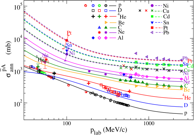
Figure 1: (Color online) Antiproton-nucleus annihilation cross sections as a function of the antiproton momentum in the laboratory, $p_{\rm lab}\equiv p_{\bar{p}{\rm lab}}$, for different nuclear targets. The solid curve for the proton target nucleus is the $\sigma_{0}/v$ phenomenological representation of the $\bar{p}p$ annihilation cross section in Eq. (27). The other curves are the results from the extended Glauber model using the basic $\bar{p}p$ annihilation cross section as input data. The solid curves are for Gaussian density distributions and the dashed curves are for uniform density distributions. The high-momentum data points are from Kuz94 . The other experimental data points are from the compilation of Bia11 , where the individual experimental sources can be found.

It should be pointed out that the $1/v$ law, Eq. (27), for the inelastic (or annihilation) cross section of slow particles is well known. It was first obtained by Bethe Bet35 and is discussed in text books Bla52 ; Lan58 ; Sat90 and other related work Won97 . It arises from multiplying the $S$-wave partial cross section, $\pi/k^{2}$, by the transmission coefficient $T_{0}$ in passing through an attractive potential well, and the transmission coefficient $T_{0}$ is proportional to $k$ at low energies. While the $1/v$ behavior is essentially an $S$-wave result, higher-$l$ partial waves will gradually contribute as the antiproton momentum reaches the GeV/$c$ region. It is nonetheless interesting to note that the simple $1/v$ law of Eq. (27) continues to provide a reasonable and efficient description of the experimental data even in the GeV/$c$ region Won11 .

Recently, an elaborate and model-independent coupled-channel partial-wave calculation, solving the problem from first principle, has been used to determine $\bar{p}$-$p$ scattering cross sections for momenta below 0.925 GeV/$c$. The calculation yields excellent agreement with the experimental $\bar{p}$-$p$ annihilation cross section for energy ranging from 0.200 to 0.925 GeV/$c$ Zhou12 . Refinement of the present $\sigma_{\rm ann}^{\bar{p}p}$ description can be made, if desired, but with additional complications.

IV Extending the Glauber Model to Low Energies

The results in Sec. II pertains to annihilation of the antiproton at high energies with straight-line trajectories. To extend the range of the application to low energies, it is necessary to forgo the assumption of straight-line trajectories. We need to take into account the modification of the trajectories due to residual Coulomb and nuclear interactions that are additional to those between the incident antiproton and an annihilated target nucleon.

The residual Coulomb and nuclear interactions affect the annihilation process in different ways. The Coulomb interaction is long-range, and the trajectory of the antiproton is attracted and pulled toward the target nucleus before the antiproton makes a contact with the nucleus [Fig. 2(a)]. It leads to a large enhancement of the annihilation cross sections at low energies Kuz94 ; Bat01 . The nuclear interaction is short-range, and it becomes operative only after coming into contact with the nucleus. The interactions modify the antiproton momentum as it travels in the nuclear interior in which $\bar{p}$-nucleon annihilation takes place. As the basic antiproton-nucleon annihilation cross section $\sigma_{\rm ann}^{\bar{p}p}$ as given by (27) is strongly momentum-dependent, we need to keep track of the antiproton momentum along the antiproton trajectory.

We shall work in the $\bar{p}$-$A$ center-of-mass system and shall measure the antiproton momentum in terms of the relative momentum $\hbox{\boldmath${p}$}_{\bar{p}A}$ defined as

$$\hbox{\boldmath${p}$}_{\bar{p}A}=\frac{m_{A}\hbox{\boldmath${p}$}_{\bar{p}}-m_{\bar{p}}\hbox{\boldmath${p}$}_{A}}{m_{\bar{p}}+m_{A}},$$ (29)

where in the center-of-mass system with $\hbox{\boldmath${p}$}_{\bar{p}}+\hbox{\boldmath${p}$}_{A}=0$, we have $\hbox{\boldmath${p}$}_{\bar{p}}=\hbox{\boldmath${p}$}_{\bar{p}A}$.

IV.1 Initial-State Coulomb Interaction

We consider the collision of an antiproton with a nucleus in the $\bar{p}A$ center-of-mass system with a center-of-mass energy $E$. The initial antiproton momentum $\hbox{\boldmath${p}$}_{\bar{p}A}$ is related to $E$ by

$$E=\frac{\hbox{\boldmath${p}$}_{{\bar{p}}A}^{2}}{2\mu}.$$ (30)

After the projectile antiproton travels along a Coulomb trajectory, it makes contact with the nucleus at $r=R_{c}$ with a momentum $\hbox{\boldmath${p}$}_{\bar{p}A}^{\prime}$ determined by

$$E = \frac{[\hbox{\boldmath${p}$}_{{\bar{p}}A}^{\prime}]^{2}}{2\mu}+V_{c}(R_{c}),$$ (31)

where $V_{c}(R_{c})$ is the Coulomb energy for the antiproton to be at the nuclear contact radius $R_{c}$,

$$V_{c}(R_{c})=-\frac{(Z_{A}-1)\alpha}{R_{c}},$$ (32)

and $Z_{A}$ is the target charge number.

The $\bar{p}p$ annihilation cross section arises from the nuclear and Coulomb interaction between the antiproton and a target proton. By employing $\sigma_{\rm ann}^{\bar{p}p}$ as the basic element in the multiple collision process in the extended Glauber model of Eq. (5), the parts of the Coulomb and nuclear interaction that are responsible for the $\bar{p}p$ annihilation have already been included. Therefore in Eq. (31) for $\bar{p}$-nucleus annihilation, we are dealing with residual interactions that are additional to those between the antiproton and the annihilated nucleon. Hence, Eq. (32) for the residual Coulomb interaction contains the coefficient ($Z_{A}-1$).

From angular momentum conservation, we have

$$p_{{\bar{p}}A}b=p_{{\bar{p}}A}^{\prime}b^{\prime}.$$ (33)

We obtain

$$b=\frac{p_{{\bar{p}}A}^{\prime}}{p_{{\bar{p}}A}}b^{\prime}.$$ (34)

From Eq. (31), we have

$$p_{{\bar{p}}A}^{\prime} = p_{{\bar{p}}A}\sqrt{1-\frac{V_{c}(R_{c})}{E}},$$ (35)

which is the relative momentum of the antiproton in the $\bar{p}A$ system at the nuclear contact radius $R_{c}$.

Starting now from the transverse coordinates $b^{\prime}$ at nuclear contact at $r=R_{c}$, one can follow the antiproton trajectory in the nuclear interior. This trajectory will be modified by residual interactions. One can evaluate a thickness function $T^{\prime}(b^{\prime})$ by integrating the nuclear density along the modified trajectory. As the thickness function $T^{\prime}(b^{\prime})$ is governed mainly the geometry of the target nucleus, we therefore expect that $T^{\prime}(b^{\prime})$ will be characterized by a length scale that will not be too different from the length scale in the thickness function $T(b^{\prime})$ without residual interactions. To the lowest order, it is reasonable to approximate $T^{\prime}(b^{\prime})$ by $T(b^{\prime})$. With such a simplifying assumption, the $\bar{p}A$ annihilation cross section at an initial antiproton momentum $p_{\bar{p}A}$ is

$$\Sigma_{\rm ann}^{\bar{p}A}(p_{\bar{p}A}) = \int d\hbox{\boldmath${b}$}\biggl{\{}1-\{1-T_{\bar{p}p}[\hbox{\boldmath${b}$}^{\prime}(\hbox{\boldmath${b}$})]\sigma_{\rm ann}^{\bar{p}p}(p_{\bar{p}A}^{\prime})\}^{Z}$$ (36)

$$\times\{1-T_{\bar{p}n}[\hbox{\boldmath${b}$}^{\prime}(\hbox{\boldmath${b}$})]\sigma_{\rm ann}^{\bar{p}n}(p_{\bar{p}A}^{\prime})\}^{N}\biggr{\}},~{}~{}~{}~{}$$

where we use a new symbol $\Sigma$ to indicate that this is the result in an extended Glauber model for $\bar{p}$-nucleus annihilation, modified to take into account the Coulomb interaction that changes the antiproton momentum from initial $p_{\bar{p}A}$ to $p_{\bar{p}A}^{\prime}$ at the nuclear contact radius $R_{c}$. We can carry out a change of variable

$$\Sigma_{\rm ann}^{\bar{p}A}(p_{\bar{p}A}) \!=\! \!\int\!\!d\hbox{\boldmath${b}$}^{\prime}\frac{bdb}{b^{\prime}db^{\prime}}\biggl{\{}1-\{1-T_{\bar{p}p}[\hbox{\boldmath${b}$}^{\prime}(\hbox{\boldmath${b}$})]\sigma_{\rm ann}^{\bar{p}p}(p_{\bar{p}A}^{\prime})\}^{Z}$$ (37)

$$\times\{1-T_{\bar{p}n}[\hbox{\boldmath${b}$}^{\prime}(\hbox{\boldmath${b}$})]\sigma_{\rm ann}^{\bar{p}n}(p_{\bar{p}A}^{\prime})\}^{N}\biggr{\}},~{}~{}~{}~{}$$

From Eqs. (34) and (35), the above Eq. (37) becomes

$$\Sigma_{\rm ann}^{\bar{p}A}(p_{\bar{p}A})=\frac{[p_{{\bar{p}}A}^{\prime}]^{2}}{p_{{\bar{p}}A}^{2}}\int d\hbox{\boldmath${b}$}^{\prime}\biggl{\{}1-\{1-T_{\bar{p}p}[\hbox{\boldmath${b}$}^{\prime}(\hbox{\boldmath${b}$})]\sigma_{\rm ann}^{\bar{p}p}(p_{\bar{p}A}^{\prime})\}^{Z}$$

$$~{}~{}~{}~{}~{}~{}~{}~{}~{}~{}~{}~{}~{}~{}~{}~{}\times\{1-T_{\bar{p}n}[\hbox{\boldmath${b}$}^{\prime}(\hbox{\boldmath${b}$})]\sigma_{\rm ann}^{\bar{p}n}(p_{\bar{p}A}^{\prime})\}^{N}\biggr{\}}$$

$$~{}~{}=\biggl{\{}1-\frac{V_{c}(R_{c})}{E}\biggr{\}}\int d\hbox{\boldmath${b}$}^{\prime}\biggl{\{}1-\{1-T_{\bar{p}p}[\hbox{\boldmath${b}$}^{\prime}(\hbox{\boldmath${b}$})]\sigma_{\rm ann}^{\bar{p}p}(p_{\bar{p}A}^{\prime})\}^{Z}$$

$$~{}~{}~{}~{}~{}~{}~{}~{}~{}~{}~{}~{}~{}~{}~{}~{}\times\{1-T_{\bar{p}n}[\hbox{\boldmath${b}$}^{\prime}(\hbox{\boldmath${b}$})]\sigma_{\rm ann}^{\bar{p}n}(p_{\bar{p}A}^{\prime})\}^{N}\biggr{\}}$$ (38)

From the results in Eq. (6), the above equation becomes

$$\Sigma_{\rm ann}^{\bar{p}A}(p_{\bar{p}A}) = \biggl{\{}1-\frac{V_{c}(R_{c})}{E}\biggr{\}}\sigma_{\rm ann}^{\bar{p}A}(\sigma_{\rm ann}^{\bar{p}p}(p_{\bar{p}A}^{\prime})).$$ (39)

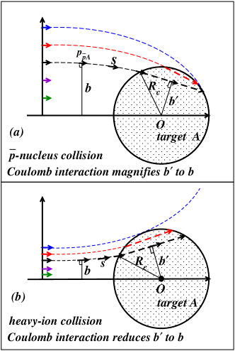
Figure 2: (Color online) Schematic picture of the bending of the antiproton trajectories $s$ as the antiproton approaches the nucleus: (a) Under the action of the attractive ${\bar{p}}$-nucleus Coulomb interaction, the impact parameter $b^{\prime}$ in the nuclear interior is magnified to the initial impact parameter $b$ which determines the annihilation cross section. (b) Under the action of a repulsive Coulomb interaction in heavy-ion collisions, the initial impact parameter $b^{\prime}$ in the nuclear interior is reduced to the initial impact parameter $b$ which determines the reaction cross section.

With the above formulation, the initial-state Coulomb interaction can be incorporated into the extended Glauber model as a mapping of the initial impact parameter $b$ to the impact parameter $b^{\prime}$ at nuclear contact. It can be pictorially depicted as a lens effect in Fig. 2. The attractive Coulomb interaction between the antiproton and the nucleus acts as a magnifying lens that magnifies the impact parameter $b^{\prime}$ at the contact radius $R_{c}$ to turn it into the initial impact parameter $b$, with which the reaction or annihilation cross section is measured [Fig. 2(a)]. The magnifying lens effect for the attractive Coulomb interaction with $b>b^{\prime}$ leads to a $\bar{p}$-nucleus annihilation cross section greater than the geometrical cross section for heavy nuclei in low-energy collisions, behaving as $[1-V_{c}(R_{c})/E]\sigma_{\rm ann}^{\bar{p}A}(\sigma_{\rm ann}^{\bar{p}p}(p_{\bar{p}A}^{\prime}))$ as given in Eq. (39), where $V_{c}(R_{c})$, the Coulomb energy at the nuclear contact radius $R_{c}$, is negative.

It is interesting to note in contrast that in heavy-ion collisions, the repulsive Coulomb initial-state interaction acts as a reducing lens that reduces the impact parameter $b^{\prime}$ at contact to become the initial impact parameter $b$ with $b<b^{\prime}$ as illustrated in Fig. 2(b). The lens effect for a repulsive Coulomb interaction leads to a reaction cross section reduced from the geometrical cross section $\pi R_{c}^{2}$ to $[1-V_{c}(R_{c})/E]\pi R_{c}^{2}$, where $V_{c}(R_{c})$ is the Coulomb energy at the Coulomb barrier and is positive Bla52 ; Won73 ; Won12 . Therefore, one obtains the unifying picture that for both the $\bar{p}$-nucleus and heavy-ion collisions, the initial-state Coulomb interaction act as a lens, leading to the same Coulomb modifying factor $[1-V_{c}(R_{c})/E]$.

IV.2 Change of the Antiproton Momentum in the Nucleus Interior

Because the basic $\bar{p}p$ annihilation cross section is strongly momentum dependent, there is, however, an additional important amendment we need to make. In the presence of the nuclear and Coulomb interactions in the nuclear interior, the antiproton momentum $p_{\bar{p}A}^{\prime}$ at the contact radius is changed to the momentum $p_{\bar{p}A}^{\prime\prime}$ in the interior of the nucleus. The $\bar{p}p$ annihilation occurs inside the nucleus at a momentum $p_{{\bar{p}}A}^{\prime\prime}$. It is necessary to modify $\Sigma_{\rm ann}^{\bar{p}p}$ in Eq. (39) to take into account this change of the antiproton momentum by replacing $p_{\bar{p}A}^{\prime}$ with $p_{\bar{p}A}^{\prime\prime}$.

The antiproton momentum $p_{{\bar{p}}A}^{\prime\prime}$ is a function of the radial position $r$ and is related to $p_{\bar{p}A}$ by the energy condition:

$$E=\frac{\hbox{\boldmath${p}$}_{{\bar{p}}A}^{2}}{2\mu}=\frac{(\hbox{\boldmath${p}$}_{{\bar{p}}A}^{\prime\prime})^{2}}{2\mu}+V_{c}(r)+V_{n}(r).$$ (40)

In order to obtain an analytical formula for general purposes for our present approximate treatment, it suffices to consider average quantities and use the root-mean-square average $\langle(\hbox{\boldmath${p}$}_{{\bar{p}}A}^{\prime\prime})^{2}\rangle^{1/2}$ given by

$$E=\frac{\langle(\hbox{\boldmath${p}$}_{{\bar{p}}A}^{\prime\prime})^{2}\rangle}{2\mu}+\langle V_{c}(r)\rangle+\langle V_{n}(r)\rangle,$$ (41)

where $\langle V_{c}(r)\rangle$ and $\langle V_{n}(r)\rangle$ are the average interior Coulomb and nuclear interactions, respectively. From the above equation, we can then approximate $p_{{\bar{p}}A}^{\prime\prime}$ by the average root-mean-squared momentum $\langle(\hbox{\boldmath${p}$}_{{\bar{p}}A}^{\prime\prime})^{2}\rangle^{1/2}$ in the interior of the nucleus,

$$p_{{\bar{p}}A}^{\prime\prime} \sim p_{{\bar{p}}A}\sqrt{1-\frac{\langle V_{c}(r)\rangle+\langle V_{n}(r)\rangle}{E}}.$$ (42)

The $\bar{p}$-nucleus annihilation cross section $\Sigma_{\rm ann}^{\bar{p}A}$ is therefore modified by changing $p_{\bar{p}A}^{\prime}$in Eq. (39) to $p_{\bar{p}A}^{\prime\prime}$ to become

$$\Sigma_{\rm ann}^{\bar{p}A}(p_{\bar{p}A}) = \biggl{\{}1-\frac{V_{c}(R_{c})}{E}\biggr{\}}\sigma_{\rm ann}^{\bar{p}A}(\sigma_{\rm ann}^{\bar{p}p}(p_{\bar{p}A}^{\prime\prime})).$$ (43)

The experimental data of $\sigma_{\rm ann}^{\bar{p}p}$ and $\Sigma_{\rm ann}^{\bar{p}A}$ are presented as a function of $p_{{\bar{p}}{\rm lab}}$ for a fixed proton or nucleus target at rest. Accordingly, we convert the antiproton momenta in the center-of-mass system in th above Eq. (43) to those in the laboratory system with fixed targets as

$$p_{\bar{p}A} = \frac{A}{A+1}p_{{\bar{p}}{\rm lab}},$$ (44)

$$p_{{\bar{p}}A}^{\prime\prime} = \frac{A}{A+1}p_{{\bar{p}}{\rm lab}}^{\prime\prime},$$ (45)

and Eq. (42) gives

$$p_{\bar{p}{\rm lab}}^{\prime\prime} = p_{\bar{p}\rm lab}\sqrt{1-\frac{\langle V_{c}(r)\rangle+\langle V_{n}(r)\rangle}{E}}.$$ (46)

Therefore, the antiproton-nucleus annihilation cross section $\Sigma_{\rm in}^{\bar{p}A}(p_{\bar{p}{\rm lab}})$ in the extended Glauber model for an antiproton with an initial momentum $p_{\bar{p}{\rm lab}}$ is given in the following compact form

$$\Sigma_{\rm ann}^{\bar{p}A}(p_{\bar{p}{\rm lab}}) = \biggl{\{}1-\frac{V_{c}(R_{c})}{E}\biggr{\}}\sigma_{\rm in}^{\bar{p}A}(\sigma_{\rm ann}^{p\bar{p}}(p_{\bar{p}{\rm lab}}^{\prime\prime})),$$ (47)

where $\sigma_{\rm in}^{\bar{p}A}(\sigma_{p\bar{p}}(p_{\bar{p}{\rm lab}}^{\prime\prime}))$ is given by Eq. (8) for light nuclei with a Gaussian thickness distribution, and by Eq. (II) for heavy nuclei with a sharp-cut-off thickness function, with the basic quantity $\sigma_{\rm ann}^{\bar{p}p}$ in Eqs. (9) or (19) evaluated at $p_{\bar{p}{\rm lab}}^{\prime\prime}$ given in terms of $p_{\bar{p}{\rm lab}}$ by Eq. (46). The Coulomb energy at contact $V_{c}(R_{c})$ is given by Eq. (32), and the average $\langle V_{c}(r)\rangle$ in the interior of the nucleus $(Z_{A},A)$ with a radius $R_{A}$ in Eq. (46) is given by

$$\langle V_{c}(r)\rangle = -3(Z_{A}-1)\alpha\left(\frac{5R^{2}_{c}-R^{2}_{A}}{10R^{3}_{c}}\right).$$ (48)

In our application of the extended Glauber model, concepts such as the contact radius $R_{c}$ and $\langle V_{c}(r)\rangle$ are simplest for a uniform density distribution. For the evaluation of these quantities in the case of small nuclei with a Gaussian thickness function, we shall approximate the Gaussian as a uniform distribution [only for the purpose of calculating $R_{c}$ and $\langle V_{c}(r)\rangle$ in Eqs. (32), (46), and (48)] with an equivalence between $R_{c}$ and $\beta$. We note that the dimensionless quantity $f$ in Eq. (9) for a Gaussian thickness function and the quantity $F$ in Eq. (19) for the sharp-cut-off distribution have the same physical meaning. It is reasonable to equate the corresponding quantities $2\pi\beta^{2}$ in Eq. (9) with the corresponding quantity $2\pi R_{c}^{2}/3$ in Eq. (19), leading to the approximate equivalence

$$R_{c}({\rm for~{}Gaussian~{}distribution})\sim\sqrt{3}\beta,$$ (49)

and similarly,

$$R_{A}({\rm for~{}Gaussian~{}distribution})\sim\sqrt{3}\beta_{A}.$$ (50)

These equivalence relations enable us to obtain the Coulomb factor $[1-V_{c}(R_{c})/E]$ in (47) and the antiproton momentum change from $p_{\bar{p}{\rm lab}}$ to $p_{\bar{p}{\rm lab}}^{\prime\prime}$ in Eq. (46), for light nuclei with Gaussian thickness functions.

V Comparison of the Extended Glauber Model with Experiment

The central results of the extended Glauber model consist of Eq. (43) or (47) and their associated supplementary equations. With the basic $\bar{p}p$ annihilation cross section $\sigma_{\rm ann}^{\bar{p}p}$ and its momentum dependence well represented from experimental data by Eq. (27), as discussed in Sec. III, it is only necessary to specify the residual nuclear interaction $\langle V_{N}\rangle$ and the nuclear geometrical parameters in Eq. (43) to obtain the $\bar{p}$-nucleus annihilation cross section. For light nuclei (with $A<40$), we use a Gaussian density distribution with the Gaussian thickness function in Eq. (6), with geometrical parameters $\beta_{A}=r_{0}^{\prime}A^{1/3}/\sqrt{3}$ and $\beta_{B}=0.68$. We find that $1.10<r_{0}^{\prime}<1.20$ fm gives a good description. For the heavy nuclei (with $A>$ 40), we use a uniform density distribution with the sharp-cut-off thickness function in Eq. (16) with geometrical parameters $R_{A}=r_{0}A^{1/3}$ and $R_{B}$ = 0.8 fm The radius parameter $r_{0}=1.04$ fm fit the data well.

In Fig. 1, the solid curve for the proton target nucleus is from the $\sigma_{0}/v$ phenomenological representation of the $\bar{p}p$ annihilation cross section in Eq. (27). The other curves are the results from the extended Glauber model using the basic $\bar{p}p$ annihilation cross section as input data. The solid curves are for Gaussian density distributions and the dashed curves are for uniform density distributions. The fitting parameters that give the theoretical $\bar{p}A$ annihilation cross sections in Fig. 1 are listed in Table I.

Table 1: Fitting parameters

Nuclei	Gaussian	Uniform	$\langle V_{n}\rangle$(MeV)
	$r^{\prime}_{0}$(fm)	$r_{0}$(fm)
2H	1.20		-1.0
4He	1.20		-4.0
Be	1.20		-10.0
C	1.20		-15.0
Ne	1.10		-25.0
Al	1.10		-30.0
Ni		1.04	-30.0
Cu		1.04	-30.0
Cd		1.04	-35.0
Sn		1.04	-35.0
Pt		1.04	-35.0
Pb		1.04	-35.0

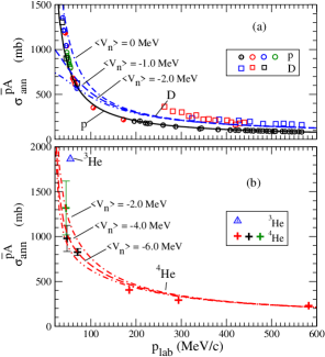
Figure 3: (Color online) $\bar{p}$ annihilation cross sections of (a) $p$ and D nuclei and (b) ⁴He nucleus. The experimental data are from Ref. Bia11 . The $\bar{p}p$ curve is from the $\sigma_{0}/v$ representation of Eq. (27), and the other curves are from the extended Glauber model.

The comparison of the extended Glauber model with the experimental data in Fig. 1 indicates that although the fits are not perfect, the extended Glauber model captures the main features of the annihilation cross sections for all energies and mass numbers. We will mention a few of the notable features of the data and the corresponding explanations in the extended Glauber model.

We examine first $\bar{p}A$ annihilation at high energies. In these high-energy annihilations, the momentum dependence of the basic $\sigma_{\rm ann}^{\bar{p}p}$ is not sensitive to the antiproton momentum change arising from the residual nuclear and Coulomb interactions $\langle V_{c}\rangle$ and $\langle V_{N}\rangle$. The initial-state Coulomb interaction energy $V_{c}(R_{c})$ is also small in comparison with the incident energy $E$. As a consequence, the corrections due to the Coulomb and nuclear interactions are small for high-energy collisions. At these high energies, the antiproton makes multiple collisions with target nucleons and probes the granular property of the nucleus when the spacing between the nucleons is large compared with the dimension of the $\bar{p}$ probe, similar to the additive quark model in meson-meson collisions Lev65 ; Won96 . The experimental $\Sigma_{\rm ann}^{\bar{p}^{2}H}/\sigma_{\rm ann}^{\bar{p}p}$ is consistently slightly greater than the theoretical prediction of $\Sigma_{\rm ann}^{\bar{p}^{2}H}/\sigma_{\rm ann}^{\bar{p}p}$$\sim$ 2. This indicates that while the Glauber model for the antiproton annihilation of the deuteron may be approximately valid, future investigations will need to include additional refinements to get a better description for the antiproton-deuteron annihilation. There are not many high-momentum data points for ⁴He, and the only high-momentum data point at 600 MeV/$c$ gives reasonable agreement with the Glauber model results.

As the number of nucleons increases in high-energy annihilations, the Glauber model results of Eqs. (8) [or (21) for $\sigma_{\rm ann}^{\bar{p}n}$$\neq$$\sigma_{\rm ann}^{\bar{p}p}$] and (II) [or (22) for $\sigma_{\rm ann}^{\bar{p}n}$$\neq$$\sigma_{\rm ann}^{\bar{p}p}$] give a $\bar{p}A$ annihilation cross section proportional to $\beta^{2}$ for a Gaussian thickness distribution and to $R_{c}^{2}$ for a uniform density distribution. Both $\beta^{2}$ and $R_{c}^{2}$ vary as $A^{2/3}$. Hence, the $\bar{p}A$ annihilation cross approaches the black-disk limit of $A^{2/3}$ limit as the nuclear mass number increases. The comparison in the high-energy region in Fig. 1 shows that the experimental data agree with predictions for nuclei across the periodic table, indicating that the experimental data indeed reach this black-disk limit of $A^{2/3}$ in the heavy-nuclei region, However, there are discrepancies for Pb at 700 MeV/$c$, which may need need to be re-checked experimentally, as the other data points for large nuclei appear to agree with theoretical predictions.

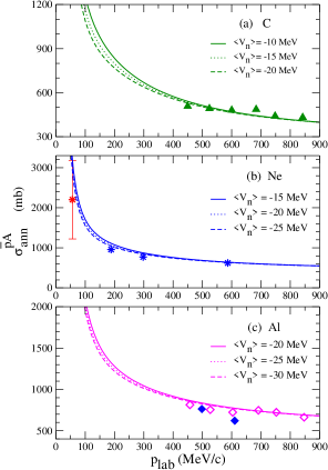
Figure 4: (Color online) $\bar{p}$ annihilation cross sections of (a) C nucleus, (b) Ne nucleus, and (c) Al nucleus. Solid curves give results from the extended Glauber model and the data points are from the compilation of Ref. Bia11 .

The situation at the low-energy region is more complicated. In addition to the multiple collision process, the Coulomb and nuclear interactions also come into play. We can examine the data for $p$, ²H, and He more closely in Fig. 3 in a linear plot in both the low and high energy regions. As shown in Figs. 1 and 3(a), the basic cross section $\sigma_{\rm ann}^{\bar{p}p}$ is of order 1000 mb at the low momentum of $p_{\bar{p}{\rm lab}}$$\sim$20 MeV/$c$, corresponding to a effective annihilation radius between $\bar{p}$ and $p$ of $R_{\bar{p}p}=(\sigma_{\rm ann}^{\bar{p}p}/\pi)^{1/2}$=6.8 fm. The large cross section and annihilation radius arise from the magnifying lens effect of the attractive initial-state Coulomb interaction that magnifies the proton radius as seen by the incoming antiproton, as discussed in Sec. III. In this case, as $R_{\bar{p}p}\gg R_{\rm deuteron}{\rm~{}or~{}}R_{\rm antiproton}$, the quantity $f$ in Eq. (8) is close to unity. According to the analysis given in Eq. (14) of Sec. III, the Glauber model with $f\sim 1$ would predict a ratio of $\Sigma_{\rm ann}^{\bar{p}^{2}H}/\sigma_{\rm ann}^{\bar{p}p}\sim 3/2$ for low-energy annihilations in the multiple collision process.

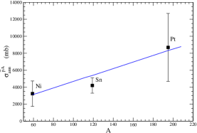
Figure 5: (Color online) $\bar{p}$ annihilation cross sections on Ni, Sn and Pt nuclei at $p_{\bar{p}{\rm lab}}$ = 100 MeV/$c$. The solid curve gives results from the extended Glauber model and the data points are from Ref. Bia11 .

Experimentally, for low-energy annihilations $\Sigma_{\rm ann}^{\bar{p}{}^{2}H}/\sigma_{\rm ann}^{\bar{p}p}$ is of order unity. In the extended Glauber model, the reduction of the ratio $\Sigma_{\rm ann}^{\bar{p}{}^{2}H}/\sigma_{\rm ann}^{\bar{p}p}$ arises from the combination of two effects: (i) the increase of the antiproton momentum inside the nucleus due to the attractive residual interactions and (ii) the momentum dependence of the basic $\sigma_{\rm ann}^{\bar{p}p}$ decreases sensitively as a function of an increase in antiproton momentum. The combined effects bring the ratio $\Sigma_{\rm ann}^{\bar{p}{}^{2}H}/\sigma_{\rm ann}^{\bar{p}p}$ from 3/2 to about unity. In Fig. 3, we show the variation of the $\bar{p}{}^{2}$H and $\bar{p}{}^{4}$He cross sections as a function of $p_{\bar{p}{\rm lab}}$ for different residual nuclear interactions $\langle V_{N}\rangle$. There is a great sensitivity of the $\bar{p}$-annihilation cross section on $V_{N}$ in the low energy region for the lightest nuclei for which the Coulomb interaction is weak. However, as the target charge number increases, the Coulomb interaction becomes stronger and the $\bar{p}$-annihilation cross section becomes less sensitive to the strength of the nuclear interaction $\langle V_{N}\rangle$, as shown in Fig. 4 for $\bar{p}$C, $\bar{p}$Ne, and $\bar{p}$Al collisions.

As the target charge number $Z$ increases further in the low-energy region, the cross section increases substantially. For example, the cross section reaches a value of about 9000 mb for the Pt nucleus, corresponding to an annihilation radius of $R_{\rm ann}=(\sigma_{\rm ann}^{\bar{p}A}/\pi)^{1/2}$=17 fm. Again, such a large annihilation radius arises from the Coulomb magnifying lens effect that magnifies the nuclear radius of Pt as seen by the incoming antiproton. The attractive Coulomb interaction as well as the nuclear interaction also changes the momentum of the antiproton inside the nucleus. The combined effect of the Coulomb initial-state interaction, the change of the antiproton momentum inside a nucleus, together with the Glauber multiple collision process of individual antiproton-nucleon annihilation, give a good description of the cross sections for the heaviest nuclei at low energies, as shown in Figs. 1 and 5.

There are only a few cases where the experimental data points deviate from the general trend and the theoretical predictions. In particular, there are discrepancies for $\bar{p}{}^{2}$H at $p_{\rm lab}$$\sim$260-600 MeV/$c$, $\bar{p}$(³He) at 55 MeV/$c$, $\bar{p}$Pb at 700 MeV/$c$, and $\bar{p}$Be at high momenta. It will be necessary to examine the origins for the discrepancies by theoretical refinements or experimental remeasurements for these cases in the future.

VI Summary and Discussions

We have extended the high-energy Glauber model to low-energy annihilation processes after taking into account the effects of Coulomb and nuclear interactions, and the change of the antiproton momentum inside a nucleus. The result is a compact equation (47) [or the equivalent (43)] with supplementary equations that capture the main features of the annihilation process and provide a simple analytical way to analyze antiproton-nucleus annihilation cross sections.

We can properly respond to the specific questions we raised in the Introduction. With respect to the mass dependence at high antiproton incident momenta, the cross sections increase almost linearly with the mass number $A$ for the lightest nuclei, but with approximately $A^{2/3}$ as the mass number increases because the basic process is a Glauber multiple collision process of the antiproton passing through a target of individual nucleons. In the low antiproton momentum region, the annihilation cross sections do not rise with $A$ as anticipated but are comparable for $p$, ²H, and He, because the residual nuclear interaction causes an increase in the antiproton momentum inside the nucleus and the increases in antiproton momentum leads to a decrease in the basic $\bar{p}$-nucleon annihilation cross section. As the charge number $Z$ increases, the initial-state Coulomb interaction magnifies the target nucleus and the $\bar{p}A$ annihilation cross section at low energies become subsequently greatly enhanced in the heavy nuclei region. With respect to the energy dependence, the energy dependence of the $\bar{p}A$ annihilation cross sections is intimately related to the energy-dependence of the $\bar{p}p$ cross sections.

The simple picture we have presented can be refined, and individual nuclear properties can be revealed, with new data that fill in the gaps in Fig. 1. The deviations of experimental data with theoretical predictions for a few cases also call for a reexamination of both the experimental measurements as well as theoretical refinements.

The extended Glauber model may find future applications in similar problems such as in the collision of mesons or baryons with nuclei at high energies as well as low energies.

Acknowledgment

This research was supported in part by the Division of Nuclear Physics, U.S. Department of Energy.

References

- (1) Green Paper, FAIR - Facility for Antiproton and Ion Research, October 2009 (unpublished).
- (2) W. Erni , (PANDA Collaboration), Euro. Phys. Jour. A 49, 25 (2013).
- (3) S. Maury, (for the AD Team), CERN Report No. CERN/PS 99-50 (HP), 1999 (unpublished).
- (4) O. Adriani et al., Nature (London) 458, 607 (2009).
- (5) M. Aguilar et al. (AMS-02 Collaboration), Phys. Rev. Lett. 110, 141102 (2013).
- (6) A. Bianconi, et al., Phys. Lett. B 704 461 (2011).
- (7) A. Bertin, et al., Phys. Lett. B 369, 77 (1996).
- (8) A. Zenoni, et al., OBELIX Collaboration, Phys. Lett. B 461, 405 (1999).
- (9) A. Zenoni, et al., OBELIX Collaboration, Phys. Lett. B 461, 413 (1999).
- (10) A. Bianconi, et al., Phys. Lett. B 481, 194 (2000).
- (11) A. Bianconi, et al., Phys. Lett. B 492, 254 (2000).
- (12) W. Brückner, et al., Z. Phys. A 335, 217 (1990).
- (13) A. Benedettini, et al., OBELIX Collaboration, Nucl. Phys. B Proc. Suppl. 56A, 58 (1997).
- (14) T.E. Kalogeropoulos, G.S. Tzanakos, Phys. Rev. D 22, 2585 (1980).
- (15) T R. Bizzarri, et al., Nuovo Cimento A 22, 225 (1974).
- (16) F. Balestra, et al., Phys. Lett. B 230, 36 (1989).
- (17) F. Balestra, et al., Phys. Lett. B 149, 69 (1984).
- (18) F. Balestra, et al., Phys. Lett. B 165, 265 (1985).
- (19) K. Nakamura, et al., Phys. Rev. Lett. 52, 731 (1984).
- (20) F. Balestra, et al., Nucl. Phys. A 452, 573 (1986).
- (21) V. Ashford, et al., Phys. Rev. C 31, 663 (1985).
- (22) V. F. Kuzichev, Yu. B. Lepikhin, V. A. Smirnitsky., Nucl. Phys. A 576, 581 (1994).
- (23) R. J. Glauber, in Lectures in Theoretical Physics, edited by W. E. Brittin and L. G. Dunham (Interscience, New York, 1959), Vol 1, p. 315.
- (24) R. Glauber and G. Matthiae, Nucl. Phys. B 21, 135 (1970).
- (25) A. Gal, E. Friedman, and C. J. Batty, Phys. Lett. B 491, 219 (2000).
- (26) C.J. Batty, E. Friedman, A. Gal, Nucl. Phys. A. 689, 721 (2001).
- (27) C. Y. Wong, Phys. Rev. D 30, 961 (1984).
- (28) C. Y. Wong, Introduction to High-Energy Heavy-Ion Collisions, (World Scientific Singapre, 1994).
- (29) C. Y. Wong and T. G. Lee, Ann. Phys. (NY) 326, 2138 (2011).
- (30) H. A. Bethe, Phys. Rev. 47, 747 (1935).
- (31) J. M. Blatt and V. F. Weisskopf, Theoretical Nuclear Physics ( John Wiley and Sons, New York, 1952), p. 349.
- (32) L. D. Landau and E. M. Lifshitz, Quantum Mechanics (Pergamon, Oxford 1958), p. 439.
- (33) G. R. Satchler, Introduction to Nuclear Reactions, 2nd Ed. (Oxford University Press, New York, London 1990, p. 121.
- (34) L. Chatterjee and C. Y. Wong, Phys. Rev. C 51, 2125 (1995).
- (35) D. Zhou, and R. G. E. Timmermans, Phys. Rev. C 86, 044003 (2012).
- (36) C. Y. Wong, Phys. Rev. Lett. 31, 766 (1973).
- (37) C. Y. Wong, Phys. Rev. C 86, 064603 (2012).
- (38) E. M. Levin and L. L. Frankfurt, JETP Lett. 2, 65 (1965); H. J. Lipkin and F. Scheck, Phys. Rev. Lett. 16, 71 (1966).
- (39) C. Y. Wong, Phys. Rev. Lett. 76, 196 (1996).