ASTEROSEISMIC ANALYSIS OF THE CoRoT TARGET HD 49933

Abstract

The frequency ratios $r_{10}$ and $r_{01}$ of HD 49933 exhibit an increase at high frequencies. This behavior also exists in the ratios of other stars, which is considered to result from the low signal-to-noise ratio and the larger linewidth at the high-frequency end and could not be predicted by stellar models in previous work. Our calculations show that the behavior not only can be reproduced by stellar models, but can be predicted by asymptotic formulas of the ratios. The frequency ratios of the Sun, too, can be reproduced well by the asymptotic formulas. The increased behavior derives from the fact that the gradient of mean molecular weight at the bottom of the radiative region hinders the propagation of p-modes, while the hindrance does not exist in the convective core. This behavior should exist in the ratios of stars with a large convective core. The characteristic of the ratios at high frequencies provides a strict constraint on stellar models and aids in determining the size of the convective core and the extent of overshooting. Observational constraints point to a star with $M=1.28\pm 0.01$ $M_{\odot}$, $R=1.458\pm 0.005$ $R_{\odot}$, $t=1.83\pm 0.1$ Gyr, $r_{cc}=0.16\pm 0.02$ $R_{\odot}$, $\alpha=1.85\pm 0.05$, and $\delta_{\rm ov}$$=0.6\pm 0.2$ for HD 49933.

1 INTRODUCTION

1.1 Determination of the Convective Core

Asteroseismology has proved to be a powerful tool for determining the fundamental parameters of stars, probing the internal structure of stars, and diagnosing physical processes in stellar interiors (Eggenberger et al., 2005, 2006; Yang & Bi, 2007b; Stello et al., 2009; Christensen-Dalsgaard & Houdek, 2010; Yang et al., 2010, 2011, 2012; Silva Aguirre et al., 2013). Stars with masses between about 1.1 and 1.5 $M_{\odot}$ have a convective core during their main sequence (MS). At the same time, however, solar-like oscillations may be present in such stars, with a convective core increasing in size during the initial stage of the MS of these stars before the core begins to shrink. The presence of the convective core brings to the fore the question of the mixing of elements in the stellar interior caused by the core’s overshooting, which prolongs the lifetime of the burning of core hydrogen by feeding more H-rich material into the core. In the current theory of stellar evolution, the overshooting of the convective core is generally described by a free parameter $\delta_{\rm ov}$. However, the uncertainty in the mass and extension of the convective core due to overshooting directly affects the determination of the global parameters of the stars by asteroseismology or other studies based on stellar evolution (Mazumdar et al., 2006). Especially for stars with a mass of around 1.1 $M_{\odot}$, there may or may not exist a convective core in their interior, depending on the input physics used in the computation of their evolutions (Christensen-Dalsgaard & Houdek, 2010). Thus determining the presence of the convective core and its extension is important for understanding the structure and evolution of stars.

There is no a direct method to determine the size of a convective core or the extension of overshooting. Fortunately, however, the low-$l$ p-modes can penetrate into the innermost layers of stars, which offers an opportunity to probe the convective core. Determining the size and extension of a convective core by means of asteroseismology was first studied by Mazumdar et al. (2006). However, for most of solar-like oscillating stars, the uncertainty of the frequencies of modes with $l=2$ and $3$ is generally larger than that of modes with $l=0$ and $1$; and the frequencies of modes with $l=3$ are usually not extracted. Thus it is difficult to obtain the quantities $\theta$ and $\eta$ defined by Mazumdar et al. (2006) or the expression suggested by Cunha & Metcalfe (2007).

The small spacings

$$d_{10}(n)\equiv-\frac{1}{2}(-\nu_{n,0}+2\nu_{n,1}-\nu_{n+1,0})$$ (1)

and

$$d_{01}(n)\equiv\frac{1}{2}(-\nu_{n,1}+2\nu_{n,0}-\nu_{n-1,1})$$ (2)

defined by Roxburgh (1993) and Roxburgh & Vorontsov (2003) can be used to diagnose the convective core of stars. In calculation, equations (1) and (2) are generally rewritten as the smoother five-point separations (Roxburgh & Vorontsov, 2003). By using this tool, Deheuvels et al. (2010) studied the solar-like pulsator HD 203608. They found that the presence or absence of a convective core in stars can be indicated by the small spacings and that the star HD 203608 with $M\simeq 0.94$ $M_{\odot}$ and $t\simeq 6.7$ Gyr in fact has a convective core. For their part, Brand$\tilde{a}$o et al. (2010) found that the slope of $d_{01}$ relates to the size of the jump in the sound speed at the edge of the convective core. De Meulenaer et al. (2010) studied the oscillations of $\alpha$ Centauri A ($1.105\pm 0.007$ $M_{\odot}$) and concluded that the $d_{01}$ allows one to set an upper limit to the amount of convective-core overshooting and that the model of $\alpha$ Centauri A with a radiative core reproduces the observed $d_{01}/\Delta\nu$ ($r_{01}$) significantly better than the model with a convective core. Furthermore, Silva Aguirre et al. (2011) analyzed the sensitivity of $r_{01}$ to the central conditions of stars during the MS evolution. They claimed that the presence of a convective core can be detected by $r_{01}$. Using this asteroseismic tool, Silva Aguirre et al. (2013) tried to detect the convective core of Perky (KIC 6106415) and Dushera (KIC 12009504). They found that the mass of Perky is $1.11\pm 0.05$ and that of Dushera is $1.15\pm 0.04$ $M_{\odot}$, and concluded that a convective core and core overshooting exist in Dushera, but could not determine whether a convective core exists in Perky.

Silva Aguirre et al. (2013) noted, moreover, that the frequency ratios $r_{01}$ and $r_{10}$ of Perky and Dushera have a sudden increase at high frequencies. They argued that this behavior results from the low signal-to-noise ratio and the larger line width at the high-frequency end and is not predicted by models. Thus they did not consider the frequency ratios on this regime in comparison with stellar models. If this behavior derives from the stellar interior structure and can be predicted by stellar models and pulsation theory, stellar models can be more strictly constrained by the ratios.

1.2 Research on HD 49933

The frequencies of p-modes of dozens of MS stars have been extracted (Appourchaux et al., 2012). The frequencies of p-modes of HD 49933, which is an F5V MS star, have been determined by many authors (Mosser et al., 2005; Appourchaux et al., 2008; Benomar et al., 2009a, b; Kallinger et al., 2010). Combing asteroseismical and non-asteroseismical data, several authors (Piau et al, 2009; Kallinger et al., 2010; Benomar et al., 2010; Creevey et al., 2011; Bigot et al., 2011) have investigated various properties of HD 49933. Piau et al (2009) concluded that the effect of rotation on HD 49933 is very weak, but that the diffusion of elements is important. Benomar et al. (2010) concluded that the overshooting of the convective core is needed, but that the microscopic diffusion may be unimportant. It seems to be difficult to reach a consensus about the mass of HD 49933. The mass determined by Piau et al (2009) is about 1.17 $M_{\odot}$; by Creevey et al. (2011) 1.1-1.2 $M_{\odot}$; by Benomar et al. (2010) 1.19 $\pm$ 0.08 $M_{\odot}$; by Bigot et al. (2011) similarly 1.20 $\pm$ 0.08 $M_{\odot}$; but by Kallinger et al. (2010) about 1.32 $M_{\odot}$. The difference in mass determinations may result from whether consideration is given to the effects of core overshooting or microscopic diffusion. In any case, depending on the difference of mass, differences in other parameters obtained by these authors obviously exist.

Because HD 49933 may be more massive than HD 203608, $\alpha$ Cen A, Perky, and Dushera, it could have a convective core. Moreover, the increase in frequency ratios $r_{01}$ and $r_{10}$ at high frequencies also exists in it, making it a good target for determining the size of a convective core by means of asteroseismology and for studying the effects of a convective core on frequency ratios. Furthermore, there are the frequency shifts of its low-degree p-modes (Salabert et al., 2011), which are understood arising from the effect of magnetic activity just as that found in the Sun. Hence, to determine the accurate stellar parameters of HD 49933 can be significant for understanding the structure and evolution of stars.

In present work, we focus mainly on determining accurate stellar parameters of HD 49933 and examining whether the increase in the frequency ratios at high frequencies can be predicted by pulsation theory and stellar models. In Section 2, we introduce our stellar models and perform a classical asteroseismic analysis. In Section 3, we show the calculated results; and in Section 4, we discuss and summarize our results.

2 STELLAR MODELS

2.1 Non-asteroseismic Observational Constraints

The luminosity of HD 49933 is 3.58 $\pm$ 0.1 $L_{\odot}$ (Michel et al., 2008; Kallinger et al., 2010), and its radius is $1.42\pm 0.04$ $R_{\odot}$ (Bigot et al., 2011). Its effective temperature is between about 6467 and 6780 K (Gillon & Magain, 2006). Combining other data, we took an average effective temperature: $T_{\rm eff}$ $=6647\pm 116$ K. HD 49933 is a slightly metal-poor star with [Fe/H] between about -0.2 and -0.5 (Gillon & Magain, 2006). For Population I stars, the ratio of surface heavy-element abundance to hydrogen abundance is related to the Fe/H by [Fe/H] $=\log(Z/X)_{s}-\log(Z/X)_{\odot}$, where $(Z/X)_{\odot}$ is the ratio of the solar mixture. The most recent ratio of the heavy-element abundance to hydrogen abundance of the Sun, $(Z/X)_{\odot}$, is 0.0171 (Asplund et al., 2004). There are, however, some discrepancies between the solar model constructed according to this new value and seismical results (Yang & Bi, 2007a). The old value of $(Z/X)_{\odot}$ is 0.023 (Grevesse & Sauval, 1998), which is in good agreement with the seismical results. The range of $(Z/X)_{s}$ for HD 49933 can be considered to be approximately between $0.0054$ and $0.0145$, i.e. $(Z/X)_{s}\approx 0.010\pm 0.005$. Considering the controversy about the value of $(Z/X)_{\odot}$, the value of $(Z/X)_{s}$ in our calculations is used as a reference, but not applied to constraining stellar models.

In order to reproduce observed characteristics of HD 49933, we computed a grid of evolutionary tracks using the Yale Rotation Evolution Code (Pinsonneault et al., 1989; Guenther et al., 1992; Yang & Bi, 2007a). The OPAL EOS tables (Rogers & Nayfonov, 2002), OPAL opacity tables (Iglesias & Rogers, 1996), and the opacity tables for low temperature provided by Ferguson et al. (2005) were used. Energy transfer by convection is treated according to the standard mixing length theory. The diffusion of both helium and heavy elements is computed by using the diffusion coefficients of Thoul et al. (1994). With the constraints mentioned above, we obtained hundreds of evolutionary tracks for HD 49933. The initial parameters of these tracks are summarized in Table 1.

2.2 Asteroseismic Observational Constraints

The low-degree p-modes of HD 49933 were first identified by Appourchaux et al. (2008) and Benomar et al. (2009a). Using longer CoRoT (Baglin et al., 2006) timeseries data of HD 49933, Benomar et al. (2009b) extracted the frequencies of the low-degree p-modes with less uncertainty. Nonetheless, the frequencies of the modes with $l=2$ still have a large error ($\sigma\gtrsim 2$ $\mu$Hz) due to the fact that these modes overlap with the $l=0$ modes and that the rotational splitting is relatively large for HD 49933 (Benomar et al., 2009b). Here we thus only used the frequencies of the modes with $l=0$ and $1$ to constrain our stellar models. For each observed frequency, we took the maximum error listed by Benomar et al. (2009b) at $1\sigma$. The average large frequency separation $\overline{\Delta\nu}$ of these modes is $85.99\pm 0.33$ $\mu$Hz.

In order to find the set of modeling parameters ($M,\alpha$, $\delta_{\rm ov}$, $Z_{i},X_{i},t$) that leads to the best agreement with the observational constraints, we computed the value of $\chi_{c}^{2}$ of models on the grid. The function $\chi_{c}^{2}$ is defined as follows

$$\chi^{2}_{c}=\frac{1}{4}\sum_{i=1}^{4}(\frac{C_{i}^{theo}-C_{i}^{obs}}{\sigma C_{i}^{obs}})^{2},$$ (3)

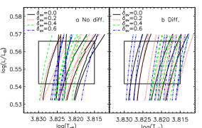
Figure 1: The Hertzsprung-Russell (H-R) diagrams of models for HD 49933. Panel $a$ shows the tracks of models without diffusion. Panel $b$ depicts the tracks of models with diffusion.

where the quantity $C_{i}^{obs}$ and $C_{i}^{theo}$ are the observed and model values of $T_{\rm eff}$, $L/L_{\odot}$, $R/R_{\odot}$, and $\overline{\Delta\nu}$, respectively. The observational uncertainty is indicated by $\sigma C_{i}^{obs}$. We obtained more than fifty tracks which are shown in Figure 1. The parameters of the models on these tracks can meet $\chi_{c}^{2}<1$. Then we computed the frequencies of low-degree p-modes of the models on these tracks using the Guenther adiabatic pulsation code (Guenther, 1994), and we calculated the value of $\chi_{\nu}^{2}$ of each model. The function $\chi_{\nu}^{2}$ is defined as follows

$$\chi_{\nu}^{2}=\frac{1}{N}\sum_{i=1}^{N}(\frac{\nu_{i}^{theo}-\nu_{i}^{obs}}{\sigma\nu_{i}^{obs}})^{2},$$ (4)

where $\nu_{i}^{obs}$ and $\nu_{i}^{theo}$ are the observed and corresponding model eigenfrequencies of the $i$th mode, respectively, and $\sigma\nu_{i}^{obs}$ is the observational uncertainty of the $i$th mode.

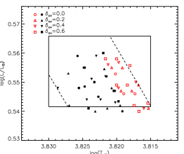
Figure 2: The locations of 50 models listed in Tables 2 and 3 in the H-R diagram. The dashed lines show the radius given by Bigot et al. (2011). Filled black symbols represent models without diffusion, while open red ones indicate models with diffusion.

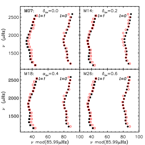
Figure 3: Echelle diagrams of models without diffusion. Filled black symbols refer to the observed frequencies, while open red ones correspond to the theoretical frequencies.

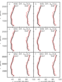
Figure 4: Same as Figure 3 but for models with diffusion.

In order to ensure that the model with the minimum $\chi_{\nu}^{2}$ is picked out as a suitable candidate, the time-step of the evolution for each track is set as small as possible when the model evolves to the vicinity of the error-box of luminosity and effective temperature in the H-R diagram. This makes the consecutive models have an approximately equal $\chi_{\nu}^{2}$. As a result, we obtained more than 50 models which are listed in Tables 2 and 3, classified according to whether the diffusion of elements is considered or not. Their positions in the H-R diagram are shown in Figure 2. For the diffusion or non-diffusion models with a given $\delta_{\rm ov}$, the model with a minimum $\chi_{\nu}^{2}$ is chosen as the candidate that best fits the model. We thus obtained four models (M07, M14, M18, and M26) in which element diffusion is not considered and four other models (M30, M35, M40, and M48) in which it is considered. The echelle diagrams of these models are shown in Figures 3 and 4.

Tables 2 and 3 show that the values of $\chi_{\nu}^{2}$ of the models M07, M14, M18, and M26 are generally smaller than those of M30, M35, M40, and M48. By comparing individual theoretical frequencies to the observed ones, the method of the $\chi_{\nu}^{2}$ minimization seems to indicate that model M26 is the one best fit for HD 49933 because it has the minimum $\chi_{\nu}^{2}$. The echelle diagram of model M26 is also slightly better than those of other models. This seems to suggest that the overshooting of the convective core is needed for HD 49933, but that the microscopic diffusion may be unimportant. These results are consistent with those obtained by Benomar et al. (2010). In addition, the mass of M26 is 1.20 $M_{\odot}$ which is also in agreement with the value of $1.19\pm 0.08$ $M_{\odot}$ determined by Benomar et al. (2010). However, Deheuvels et al. (2010) and Silva Aguirre et al. (2013) have pointed out that the most fitting model as found solely by matching individual frequencies of oscillations does not always properly reproduce the ratios $r_{01}$ and $r_{10}$, i.e., the interior structure of the “best-fit model” may not match the interior structure of the star.

2.3 The Effect of Near-surface Correction on $\chi_{\nu}^{2}$

There is a well-known near-surface effect in heliosismology. A similar effect must occur as well in asteroseismology (Kjeldsen et al., 2008), which could affect results when one compares theoretical individual frequencies to observed ones. An empirical formula was proposed by Kjeldsen et al. (2008) to correct the near-surface effect for models of solar-like stars. When we calculated the values of $\chi_{\nu}^{2}$ listed in Tables 2 and 3, such a correction was not taken into account.

In order to understand the effect of the surface correction on all computed models, we calculated the chi squared after frequency correction ($\chi^{2}_{\nu_{\mathrm{corr}}}$), using equations (6) and (2) of Kjeldsen et al. (2008). For a given $\delta_{\rm ov}$, the surface correction does not change the “best candidate” (see Table 2 and 3). However in overall and for models without diffusion, while a model with a 0.2 overshoot was favored (M14), a model with no overshoot is now favored (M07). Nonetheless, according to the theory of Kjeldsen et al. (2008), one should also account of the correction factor $r_{f}$ to define the best model. The closer a reference model is to the best one, the closer to $1$ is $r_{f}$. In other words, the uncorrected and corrected chi squared must be the same and small. The value of the correction factor $r_{f}$ is $1.00031$ for M14, which among all our models, is the closest to one. For models with diffusion, we favor M48 because of its $\chi^{2}_{\nu_{\mathrm{corr}}}$ and because $r_{f}=1.00038$. We therefore conclude that M14 and M48 are the best models that fit the observations.

3 ASTEROSEISMICAL DIAGNOSIS

3.1 The Frequency Ratios of Models

We calculated the ratios $r_{01}$ and $r_{10}$ of the observed and theoretical frequencies. Figure 5 shows that the observed $r_{01}$ and $r_{10}$ decrease with a frequency in the approximate range between about 1300 and 2050 $\mu$Hz (hereafter labeled “decrease range”), but they increase with a frequency in the range between about 2050 and 2400 $\mu$Hz (labeled “increase range”). The model M14 cannot reproduce the observed ratios $r_{01}$ and $r_{10}$. However, models M26, M40, and M48 reproduce well the ratios in the decrease range. The same ratios of models M26 and M40 decrease in the increase range, which is inconsistent with the observed results; but those of model M48 increase slightly in the range between about 2100 and 2500 $\mu$Hz. Although the ratios of M48 cannot reproduce the increase at high frequencies, the trend of increase is consistent with the behavior of the observed ratios. Furthermore, Figure 5 shows that the observed $r_{01}$ is slightly larger than $r_{10}$ in the decrease range, but smaller in the increase range. The ratios of M48 exhibit the same characteristics.

Models M26 and M48 have a large $\delta_{\rm ov}$. The increase behavior of the frequency ratios at high frequencies might be related to the convective core, which can be significantly affected by overshooting parameter $\delta_{\rm ov}$. Thus we constructed four models with a larger $\delta_{\rm ov}$, i.e. M51, M52, M53, and M54. These reproduce not only the ratios in the decrease range, but also the increase behavior of the ratios at high frequencies (see Figure 6). In addition, the ratio $r_{01}$ of these models is larger than their $r_{10}$ at low frequencies, but smaller at high frequencies. The increase in the ratios $r_{01}$ and $r_{10}$ for these models is more obvious at high frequencies. The behavior of the increase could derive from the interior structure of stars.

3.2 Asymptotic Formula and Modification

3.2.1 Asymptotic Formula of Frequency Ratios

In order to better understand whether the increase behavior results from the structure of stars or not, we analyze the characteristics of the ratios by making use of the asymptotic formula of frequencies. That for the frequency $\nu_{n,l}$ of a stellar p-mode of order n and degree l is given by Tassoul (1980) and Gough & Novotny (1990) as

$$\nu_{n,l}\simeq(n+\frac{l}{2}+\varepsilon)\nu_{0}-[Al(l+1)-B]\nu_{0}^{2}\nu_{n,l}^{-1}$$ (5)

for $n/(l+\frac{1}{2})\rightarrow\infty$, where

$$\nu_{0}=(2\int_{0}^{R}\frac{dr}{c})^{-1}$$ (6)

and

$$A=\frac{1}{4\pi^{2}\nu_{0}}[\frac{c(R)}{R}-\int_{r_{t}}^{R}\frac{1}{r}\frac{dc}{dr}dr].$$ (7)

In this equation c is the adiabatic sound speed at radius r and R is the fiducial radius of the star; $\varepsilon$ and B are the quantities that are independent of the mode of oscillation, but depend predominantly on the structure of the outer parts of the star; $r_{t}$ is the inner turning point of the mode with the frequency $\nu_{n,l}$ and can be determined by

$$\frac{c(r_{t})}{r_{t}}=\frac{2\pi\nu_{n,l}}{\sqrt{l(l+1)}};$$ (8)

$\nu_{0}$ is related to the travel time of sound across the stellar diameter; $A$ is a measure of the sound-speed gradient and is most sensitive to conditions in the stellar core and to changes in the composition profile (Gough & Novotny, 1990; Christensen-Dalsgaard, 1993).

Using this asymptotic formula, one can obtain

$$d_{10}(n)=\frac{1}{2}[4A\nu_{0}^{2}\nu_{n,1}^{-1}-B\nu_{0}^{2}(2\nu_{n,1}^{-1}-\nu_{n,0}^{-1}-\nu_{n+1,0}^{-1})]$$ (9)

and

$$d_{01}(n)=\frac{1}{2}[2A\nu_{0}^{2}(\nu_{n,1}^{-1}+\nu_{n-1,1}^{-1})+B\nu_{0}^{2}(2\nu_{n,0}^{-1}-\nu_{n,1}^{-1}-\nu_{n-1,1}^{-1})].$$ (10)

The quantities $A$ and $B$ have the same order [see equation (72) of Tassoul (1980)]. Because $2\nu_{n,1}^{-1}\gg|2\nu_{n,1}^{-1}-\nu_{n,0}^{-1}-\nu_{n+1,0}^{-1}|$ and $\nu_{n,1}^{-1}+\nu_{n-1,1}^{-1}\gg|2\nu_{n,0}^{-1}-\nu_{n,1}^{-1}-\nu_{n-1,1}^{-1}|$, then

$$d_{10}(n)\simeq A\nu_{0}^{2}2\nu_{n,1}^{-1}$$ (11)

and

$$d_{01}(n)\simeq A\nu_{0}^{2}(\nu_{n,1}^{-1}+\nu_{n-1,1}^{-1}).$$ (12)

Using $\Delta\nu\simeq\nu_{0}$, we can get

$$r_{10}(n)\equiv\frac{d_{10}(n)}{\Delta\nu}\simeq A\nu_{0}2\nu_{n,1}^{-1}$$ (13)

and

$$r_{01}(n)\equiv\frac{d_{01}(n)}{\Delta\nu}\simeq A\nu_{0}(\nu_{n,1}^{-1}+\nu_{n-1,1}^{-1}),$$ (14)

where

$$A\nu_{0}=\frac{1}{4\pi^{2}}[\frac{c(R)}{R}+\int_{r_{t}}^{R}(-\frac{1}{r}\frac{dc}{dr})dr].$$ (15)

The quantity $1/\nu_{n,1}$ decreases monotonically with the increase in frequencies. Thus, the sudden change in the ratios could result from the change in $A\nu_{0}$.

3.2.2 Characteristics Predicted by the Asymptotic Formula

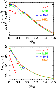
Figure 7: The radial distributions of adiabatic sound speed and quantity $A\nu_{0}$ of different models.

The radial distributions of the adiabatic sound speed and the quantity $A\nu_{0}$ of different models are shown in Figure 7. The quantity $A\nu_{0}$ increases with the decrease in radius and depends mainly on the conditions in the stellar core. According to equation (8), the higher the frequencies, the smaller the $r_{t}$ for modes with a given $l$. Thus the quantity $A\nu_{0}$ increases with increasing frequencies. When the decrease of $2/\nu_{n,1}$ cannot counteract the increase of $A\nu_{0}$, the ratio $r_{10}$ would increase with increasing frequencies.

Moreover, if changes in the ratios $r_{10}$ and $r_{01}$ are dominated mainly by the changes of $2/\nu_{n,1}$ and ($1/\nu_{n,1}+1/\nu_{n-1,1}$) respectively, equations (13) and (14) show that the ratios decrease with increasing frequencies and that $r_{01}$ can be slightly larger than $r_{10}$ because $(1/\nu_{n,1}+1/\nu_{n-1,1})>2/\nu_{n,1}$. This case happens at low frequencies because the lower the frequency, the larger the difference between $1/\nu_{n,1}$ and $1/\nu_{n-1,1}$. However, if the changes in the ratios are mainly dominated by the changes of $A\nu_{0}$ and the difference between $1/\nu_{n,1}$ and $1/\nu_{n-1,1}$ can be neglected, the ratios increase with the increase in $A\nu_{0}$, and $r_{01}$ would be slightly smaller than $r_{10}$ because the $A\nu_{0}$ corresponding to $\nu_{n-1,1}$ is smaller than that corresponding to $\nu_{n,1}$. This case occurs at high frequencies because the higher the frequency, the smaller the difference between $1/\nu_{n,1}$ and $1/\nu_{n-1,1}$. These characteristics are similar to those of the ratios of the observed frequencies and the adiabatic oscillation frequencies of models M48, M51, M52, M53, and M54. Thus an increase could exist in the ratios of p-mode frequencies of a star, and it could be seen within the observed frequency range of the star, provided that the slope change is close to the frequencies of the maximum seismical amplitude ($\nu_{max}$).

Figure 7 shows that the quantity $A\nu_{0}$ varies significantly with the stellar radius in the convective core, which may lead to the possibility that the ratios $r_{10}$ and $r_{01}$ increase with increasing frequencies. By making use of asymptotic formulas (8) and (13), our calculations show that the ratios of M07 exhibit an insignificant increase at high frequencies [see the dotted (blue) line in the panel M07 of Figure 8], which shows that the increase in ratios can be predicted by the asymptotic formulas despite the fact that the increase cannot match the observed one. However, the ratio of the adiabatic oscillation frequencies of M07 (the green dash-dotted line) does not exhibit a similar behavior.

3.2.3 Modification to the Formula

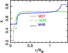
Figure 9: The radial distributions of hydrogen abundance of different models.

The value of $r_{10}$ and $r_{01}$ computed using the asymptotic formulas (13) and (14) strongly depend on the equation (8), which is obtained from the dispersion relation of p-modes. The dispersion relation is deduced from adiabatic oscillation equations with the conditions of Cowling approximation and local (constant coefficient) approximation (Unno et al., 1989). For stars with a convective core, there is a large gradient of chemical composition $\nabla_{\mu}$ at the top of the core (see Figure 9), which leads to a sudden increase in the squared Brunt-V$\ddot{a}$is$\ddot{a}$l$\ddot{a}$ frequency $N^{2}$. This results in the fact that the coefficient {$h(r)=\exp[\int^{r}_{0}(N^{2}/g-g/c^{2})dr]$} of the adiabatic oscillation equations [(15.5) and (15.6) in Unno et al. (1989)] strongly depends on radius $r$ in this region; i.e. the coefficients should not be assumed to be constant. Thus relation (8) should be modified. Moreover, the large $\nabla_{\mu}$ might hinder the fact that p-modes transmit in the stellar interior. In other words, the equation (8) might underestimate the value of the turning point $r_{t}$. Therefore, we modify relation (8) as

$$\nu_{n,l}=f_{0}\frac{c(r_{t})}{r_{t}}\frac{\sqrt{l(l+1)}}{2\pi},$$ (16)

where the parameter $f_{0}$ is larger than one. For a given mode, the position of the turning point determined by equation (8) is deeper than that predicted by equation (16). Thus the frequency ratios computed by equations (13) and (8) are larger than those calculated by equations (13) and (16).

3.3 Calculated Results of Asymptotic Formula

3.3.1 Results of HD 49933

The observed $r_{10}$ has an increase at about 2050 $\mu$Hz. If the increase is related to the convective core, we can use the asymptotic formulas (13) and (16) and the structure of model M48 to calibrate equation (16) and determine that the value of $f_{0}$ is 2.0. The solid (cyan) lines in Figure 8 show the computed $r_{10}$ using formulas (13) and (16). For M07, equation (16) predicts that modes with a frequency between 1000 and 2500 $\mu$Hz cannot reach the convective core. Thus the ratio $r_{10}$ of adiabatic oscillation frequencies in this range does not exhibit increased behavior. For M26 and M52, Figure 8 shows that the ratio $r_{10}$ of adiabatic oscillation frequencies starts to increase at about 2400 and 2000 $\mu$Hz respectively. Formulas (13) and (16) predict that modes with a frequency larger than about 2300 $\mu$Hz for M26 and 1950 $\mu$Hz for M52 can reach the convective core. Unfortunately, the ratio $r_{10}$ determined by formulas (13) and (16) does not reproduce directly the observed increase behavior.

3.3.2 Further Assumption and Results

In a convective region, there is no gradient of chemical composition; so the turning point should be determined by equation (8). Due to the fact that the quantity $A\nu_{0}$ is mainly dependent on the conditions in stellar interiors, we assume that the turning point of the modes propagating out of the convective core is determined by equation (16) despite the fact that there is no chemical gradient in the outer layers of the radiative region, but that the turning point of the modes penetrated the convective core is determined by equation (8). These assumptions can result in two inferences. One is that the frequency ratios can increase suddenly near the frequencies whose corresponding turning points are located at the boundary of the convective core. The other is that the magnitude of the increase is equal to the difference between the ratios determined by equations (13) and (8) and those determined by equations (13) and (16) at the boundary of the convective core.

For model M48, according to formula (16), the turning point of the modes of about 2100 $\mu$Hz is located at the boundary of the convective core. For the modes with frequencies larger than 2100 $\mu$Hz, their turning points should be determined by equation (8) in the convective core. The value of $r_{10}$ determined by formulas (13) and (8) is about 0.0494 at around 2100 $\mu$Hz, while that determined by formulas (13) and (16) is about 0.0323 for the frequency just less than 2100 $\mu$Hz. The difference between these two values is about 0.017, which is compatible with the value of 0.019 of the increase of the observed $r_{10}$ at around 2100 $\mu$Hz. A sudden change in the turning point of the consecutive $\nu_{n,1}$ seems unreasonable. Thus we assume that the overshooting region is a transition region between the radiative region and the convective core as determined by Schwarzschild criteria; that is to say, the value of $f_{0}$ changes from 2.0 to 1.0 in the overshooting region. The ratios $r_{10}$ computed according to this assumption are shown by the long-dashed (magenta) lines in Figure 8. The magnitude of the increase of the $r_{10}$ between about 2050 and 2250 $\mu$Hz is about 0.015 for M48, which is slightly lower than the observed value of 0.019. For M52, when the overshooting region is treated as a transition region, the magnitude of the increase in the $r_{10}$ between 1950 and 2150 $\mu$Hz is also about 0.015.

3.3.3 Test by the Sun

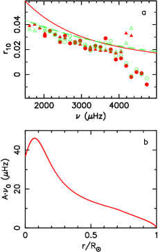
Figure 10: Panel $a$: The solid red and open green circles show the $r_{01}$ and $r_{10}$ of the Sun (Duvall et al., 1988), while the $r_{01}$ and $r_{10}$ of the Sun (García et al., 2011) are indicated by the solid red and open green triangles, respectively. The solid red line represents the ratio $r_{10}$ computed using solar model M98 (Yang & Bi, 2007a) and equations (13) and (8); the dashed green line depicts the ratio $r_{10}$ computed using solar model M98 and equations (13) and (16). Panel $b$ indicates the distribution of $A\nu_{0}$ of model M98. The turning point of 4000 $\mu$Hz is located at about 0.082 $R_{\odot}$.

There exists a gradient of the mean molecular weight in the interior of the Sun despite the fact that it is less than the gradient in stars with a convective core. Thus the calibrated equation (16) can be tested by the solar model and solar oscillation frequencies. We computed the ratios $r_{10}$ and $r_{01}$ of the Sun from the frequencies given by Duvall et al. (1988) and García et al. (2011) (see the panel $a$ of Figure 10) respectively, and the values of the asymptotic $r_{10}$ for the solar model M98 (Yang & Bi, 2007a). The solid (red) line in the panel $a$ of Figure 10 shows the $r_{10}$ computed using equations (13) and (8). The dashed (green) line represents the $r_{10}$ computed using equations (13) and (16), which is in good agreement with the observed $r_{10}$ between about 2000 and 3700 $\mu$Hz for the frequencies calculated by Duvall et al. (1988) or between about 1500 and 4000 $\mu$Hz for those calculated by García et al. (2011).

However, the asymptotic formulas do not reproduce the observed $r_{10}$ when frequencies are larger than 4000 $\mu$Hz. In this range, the value of the asymptotic $r_{10}$ is larger than that obtained from the frequencies of Duvall et al. (1988), but lower than that obtained from those of García et al. (2011). According to equation (16), the turning point $r_{t}$ of the modes of 4000 and 4800 $\mu$Hz is located at about 0.082 and 0.069 $R_{\odot}$, respectively. Panel $b$ of Figure 10 shows that the quantity $A\nu_{0}$ reaches the maximum at about 0.07 $R_{\odot}$. Then the quantity decreases with decreasing radius; i.e., $A\nu_{0}$ decreases with the increase in frequencies when the frequencies are larger than a certain value, which leads to the fact that the ratios of the modes propagating in this region could decrease more rapidly with the increase in frequencies. The discrepancy between the observed $r_{10}$ and the asymptotic $r_{10}$ at high frequencies could reflect that between the central structure of the solar model and that of the Sun.

3.4 The Influence of Near-surface Effects on the Ratios

In principle, the ratios $r_{10}$ and $r_{01}$ should not be sensitive to surface effects. In order to determine whether they are actually affected by such effects, we computed the ratios of the corrected frequencies of our all models. The ratio $r_{10}$ of the corrected frequencies of models M07, M26, M48, and M52 is shown in Figure 8 by the dash-triple-dotted (orange) line, which completely overlaps with the uncorrected one. Our calculations show that the ratios $r_{10}$ and $r_{01}$ are not affected by such effects.

4 DISCUSSIONS AND SUMMARY

4.1 Discussions

Silva Aguirre et al. (2011) argued that the slope of the ratios $r_{10}$ and $r_{01}$ depends simultaneously on the central hydrogen content ($X_{c}$), the extent of the convective core, and the amplitude of the sound-speed discontinuity at the core boundary. Brand$\tilde{a}$o et al. (2010) also concluded that the relation between the slope of $d_{01}$ and the size of the jump in the sound speed at the edge of the convective core is linear. In our models, however, the slope seems not to depend directly on the central hydrogen content, the extent of the convective core, or the size of the jump in the sound speed. Model M26 has almost the steepest ratios in the observable range of frequencies (see Figure 8). However, its central hydrogen content and the size of its convective core are larger than those of model M07, though less than those of M48. At the same time the amplitude of the sound-speed discontinuity at the core boundary (see Figure 7) is less than that of M07, but larger than that of M48.

According to equation (13), due to the fact that $2/\nu_{n,1}$ decreases with increasing frequencies, the slope of ratio $r_{10}$ is mainly affected by $A\nu_{0}$. If a mode did not arrive at the convective core, its $A\nu_{0}$ could not be affected by that core. According to equation (16), the value of $A\nu_{0}$ is about 28.7 $\mu$Hz at 1300 $\mu$Hz for models M07 and M26; but that value is about 40.7 $\mu$Hz at 2400 $\mu$Hz, whose corresponding turning point is located in the radiative region for M07. Thus the $r_{10}$ of model M07 only slightly decreases with the increase in frequencies and is not affected by the jump in the sound speed at the core boundary. For model M26, the value is 32.6 $\mu$Hz at 2300 $\mu$Hz, whose corresponding turning point is located just at the core boundary; in this case the jump in the sound speed at the core boundary affects the slope of $r_{10}$ of adiabatic frequencies.

The overshooting region is treated as a transition area between the radiative region and the convective core, which means that the mixing should not be a complete process in the overshooting region. This is consistent with the result that overshooting mixing should be regarded as a weak mixing process in stars (Zhang, 2012, 2013).

The distribution of $r_{10}$ obtained from the asymptotic formula has a shift, compared to the distributions of the observed $r_{10}$ (see Figure 8). This may suggest that there are some discrepancies between our models and HD 49933.

Moreover, the uncertainty of the observed ratios is relatively large at high frequencies, which is mainly due to the uncertainty of the $l=0$ modes. Considering the large uncertainty, the increase of the ratios is not very significant. This may affect our interpretation on HD 49933.

In our calculations, only the models with a large convective core can reproduce the increase in the ratios $r_{10}$ and $r_{01}$. For these models, the value of $\delta_{\rm ov}$ is around 0.6, which is larger than the generally accepted value. This may be why the behavior cannot be predicted by the models of Silva Aguirre et al. (2013). Moreover, the surface rotation period of HD 49933 is about 3.4 days (Benomar et al., 2009b), which is obviously lower than the approximately 27 days of the Sun. Rotation can lead to an increase in the convective core, which depends on the rotational mixing and rotation rate (Maeder, 1987; Yang et al., 2013a). Thus, the large core might be related to the rotation. In addition, the low-mass stars with mass more massive than about 1.25 $M_{\odot}$ have a shallow convective zone. Their angular momentum loss rate could be either lower than that of the Sun or neglected (Ekstr$\ddot{o}$m et al., 2012; Yang et al., 2013a, b). The rotation rate of such stars can obviously be higher than that of the Sun. The high rotation rate of HD 49933, therefore, suggests that its mass might be greater than 1.25 $M_{\odot}$.

4.2 Summary

In this work, we constructed a series of models for HD49933. The increase behavior in the ratios $r_{10}$ and $r_{01}$ at high frequencies is not only reproduced by our models, but also predicted by the asymptotic formulas of the ratios. The increase in the ratios could exist for stars with a large convective core and derive from the fact that the gradient of chemical compositions at the bottom of the radiative region hinders the propagation of p-modes, while such a hindrance does not exist in the convective core. The asymptotic formulas of the ratios calibrated to HD 49933 reproduce well the solar ratios between about 1500 and 4000 $\mu$Hz. At higher frequencies, the behavior of the ratios obtained from the frequencies of García et al. (2011) is contrary to that obtained from the data of Duvall et al. (1988); at the same time, the observed ratios cannot be reproduced by theoretical ratios.

When the characteristic of the increase in the ratios is neglected, the observational constraints point to a star with $M=1.20^{+0.09}_{-0.02}$ $M_{\odot}$, $R=1.43^{+0.033}_{-0.013}$ $R_{\odot}$, $t=2.97^{+0.06}_{-1.24}$ Gyr, $r_{cc}=0.145^{+0.035}_{-0.023}$ $R_{\odot}$, $\alpha=1.85\pm 0.05$, and $\delta_{\rm ov}$$=0.6\pm 0.2$ for HD 49933, where the uncertainties correspond to the maximum/minimum values reached by the model parameters, for $1\sigma$ departures from the most probable value of the observational constraints. However, when that characteristic is used to constrain stellar models, the observational constraints favor a star with $M=1.28\pm 0.01$ $M_{\odot}$, $R=1.458\pm 0.005$ $R_{\odot}$, $t=1.83\pm 0.1$ Gyr, $r_{cc}=0.16\pm 0.02$ $R_{\odot}$, $\alpha=1.85\pm 0.05$, and $\delta_{\rm ov}$$=0.6\pm 0.2$. The characteristic of the increase in the ratios provides a strict constraint on stellar models and could be applied to determining the extent of overshooting and the size of the convective core. Moreover, in order to reproduce the characteristic of the increase in the ratios of HD 49933, the diffusion of chemical elements and the core overshooting are required. However, if the frequency ratios at high frequencies are not considered when compared to stellar models, the effect of element diffusion can be neglected when computing the models.

Figure 5: The ratios $r_{01}$ and $r_{10}$ of observational frequencies and adiabatic frequencies of models. The red shows $r_{01}$. The green represents $r_{10}$. For each frequency, we accepted the maximum error bar listed by Benomar et al. (2009b) at $1\sigma$.

Figure 6: Same as the Figure 5, but for different models.

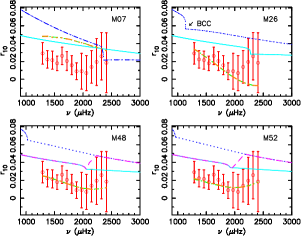
Figure 8: The ratio $r_{10}$ as a function of oscillation frequencies. The circles with an error bar show the observed data. The dash-dotted green line indicates the ratio of adiabatic oscillation frequencies. The dotted blue line shows the ratio computed from equations (13) and (8). The solid cyan line depicts the ratio computed using equations (13) and (16). The long-dashed magenta line represents the one computed using equations (13) and (16) in the radiative region, but computed using equations (13) and (8) in the convective core, while the overshoot region has been treated as a transition region. The dash-triple-dotted orange line depicts the ratio for the corrected adiabatic oscillation frequencies. It overlaps with the uncorrected one. The BCC shows the boundary of the convective core.

Table 1: The initial parameters of models.

	Variable	Minimum	Maximum	$\delta$
	M/M⊙	1.10	1.34	$\leq$0.02
	$\alpha$	1.65	1.95	$\leq$0.1
	$\delta_{\rm ov}$	0.0	0.6	$\leq$0.2
Diffusion	$Z_{i}$	0.006	0.030	0.002
	$X_{i}$	0.675	0.699	0.002
No Diff.	$Z_{i}$	0.004	0.012	0.002
	$X_{i}$	0.713	0.721	0.002

Table 2: Parameters of models without diffusion. The models with the same $\delta_{\rm ov}$ are treated as a set. In each set, the model with a minimum $\chi_{\nu}^{2}$ is highlighted by italics. The $r_{cc}$ shows the radius of the convctive core of a model.

Model	$M$	$(Z/X)_{s}$	$X_{c}$	$T_{\rm eff}$	$L$	$r_{cc}$	$R$	age	$\alpha$	$\delta_{\rm ov}$	$\Delta\nu$	$\chi_{\nu}^{2}$	$\chi^{2}_{\nu_{\mathrm{corr}}}$	$\chi_{c}^{2}$
	($M_{\odot}$)			(K)	($L_{\odot}$)	($R_{\odot}$)	($R_{\odot}$)	(Gyr)			($\mu$Hz)
M1	1.14	0.0112	0.020	6679	3.592	0.042	1.417	2.978	1.75	0.0	86.48	9.47	14.65	0.86
M2	1.18	0.0140	0.079	6648	3.508	0.031	1.414	2.681	1.75	0.0	86.43	6.86	10.63	0.57
M3	1.18	0.0140	0.044	6681	3.589	0.078	1.417	2.764	1.85	0.0	86.33	5.57	7.49	0.30
M4	1.20	0.0140	0.206	6695	3.631	0.062	1.418	2.397	1.75	0.0	86.45	10.00	14.47	0.59
M5	1.22	0.0168	0.267	6594	3.467	0.070	1.429	2.269	1.65	0.0	86.45	9.77	14.37	0.86
M6	1.22	0.0168	0.238	6611	3.524	0.071	1.433	2.382	1.75	0.0	86.27	8.47	6.92	0.31
M7	1.22	0.0168	0.226	6626	3.573	0.073	1.436	2.460	1.85	0.0	86.19	4.56	2.75	0.14
M8	1.10	0.0083	0.166	6714	3.483	0.074	1.381	3.406	1.85	0.2	86.35	8.15	9.86	0.85
M9	1.14	0.0112	0.223	6655	3.467	0.083	1.403	3.125	1.85	0.2	86.28	7.82	7.41	0.55
M10	1.16	0.0112	0.286	6716	3.573	0.088	1.399	2.692	1.75	0.2	86.50	12.86	16.80	0.75
M11	1.18	0.0140	0.294	6628	3.475	0.091	1.416	2.718	1.75	0.2	86.40	5.43	9.39	0.67
M12	1.22	0.0168	0.364	6599	3.483	0.098	1.429	2.290	1.65	0.2	86.41	13.30	15.88	0.69
M13	1.22	0.0168	0.341	6618	3.532	0.097	1.433	2.398	1.75	0.2	86.39	5.40	10.28	0.47
M14	1.22	0.0168	0.319	6635	3.589	0.097	1.435	2.497	1.85	0.2	86.27	2.50	3.00	0.23
M15	1.14	0.0112	0.341	6674	3.499	0.115	1.401	3.202	1.85	0.4	86.29	5.86	8.25	0.44
M16	1.16	0.0112	0.385	6726	3.606	0.120	1.400	2.776	1.75	0.4	86.57	10.84	21.75	0.97
M17	1.18	0.0140	0.390	6643	3.499	0.123	1.415	2.785	1.75	0.4	86.39	6.68	11.94	0.53
M18	1.18	0.0140	0.375	6663	3.556	0.122	1.417	2.877	1.85	0.4	86.30	2.71	4.19	0.25
M19	1.22	0.0168	0.439	6610	3.491	0.127	1.427	2.331	1.65	0.4	86.55	9.59	17.86	0.95
M20	1.22	0.0168	0.423	6632	3.565	0.127	1.431	2.451	1.75	0.4	86.37	6.77	11.83	0.36
M21	1.22	0.0168	0.407	6652	3.622	0.128	1.434	2.554	1.85	0.4	86.25	3.56	5.73	0.23
M22	1.14	0.0112	0.412	6670	3.475	0.140	1.397	3.215	1.75	0.6	86.47	8.37	17.84	0.89
M23	1.14	0.0112	0.400	6692	3.532	0.138	1.399	3.304	1.85	0.6	86.46	9.06	11.67	0.67
M24	1.18	0.0140	0.440	6657	3.548	0.145	1.414	2.882	1.75	0.6	86.45	7.23	16.29	0.52
M25	1.18	0.0140	0.427	6679	3.589	0.145	1.417	2.979	1.85	0.6	86.35	4.36	9.88	0.32
M26	1.20	0.0168	0.430	6603	3.491	0.1454	1.431	2.972	1.85	0.6	86.45	1.99	3.79	0.74
M27	1.20	0.0168	0.423	6613	3.526	0.1449	1.433	3.028	1.90	0.6	86.17	2.33	3.61	0.19
M28	1.22	0.0168	0.458	6637	3.631	0.150	1.445	2.609	1.75	0.6	86.39	7.66	10.09	0.53

Table 3: Same as Table 2, but for models with diffusion.

Model	$M$	$(Z/X)_{s}$	$X_{c}$	$T_{\rm eff}$	$L$	$r_{cc}$	$R$	age	$\alpha$	$\delta_{\rm ov}$	$\Delta\nu$	$\chi_{\nu}^{2}$	$\chi^{2}_{\nu_{\mathrm{corr}}}$	$\chi_{c}^{2}$
	($M_{\odot}$)			(K)	($L_{\odot}$)	($R_{\odot}$)	($R_{\odot}$)	(Gyr)			($\mu$Hz)
M29	1.26	0.0062	0.405	6591	3.516	0.087	1.440	1.484	1.75	0.0	86.45	8.22	14.74	0.71
M30	1.26	0.0076	0.383	6610	3.573	0.088	1.443	1.596	1.85	0.0	86.33	5.45	8.31	0.38
M31	1.28	0.0087	0.417	6566	3.516	0.091	1.450	1.433	1.75	0.0	86.39	6.68	11.35	0.73
M32	1.26	0.0062	0.465	6597	3.524	0.113	1.439	1.494	1.75	0.2	86.45	8.64	16.34	0.67
M33	1.26	0.0074	0.446	6618	3.589	0.113	1.443	1.603	1.85	0.2	86.32	5.87	9.52	0.34
M34	1.28	0.0085	0.475	6573	3.524	0.117	1.450	1.440	1.75	0.2	86.41	6.87	12.40	0.73
M35	1.28	0.0099	0.454	6594	3.589	0.117	1.416	1.554	1.85	0.2	86.29	4.30	6.79	0.26
M36	1.30	0.0092	0.505	6536	3.475	0.120	1.454	1.246	1.65	0.2	86.48	9.00	17.03	1.23
M37	1.30	0.0108	0.483	6558	3.540	0.119	1.459	1.372	1.75	0.2	86.36	5.83	10.13	0.74
M38	1.26	0.0061	0.509	6603	3.532	0.141	1.439	1.536	1.75	0.4	86.44	9.46	18.39	0.62
M39	1.26	0.0073	0.494	6626	3.597	0.140	1.441	1.639	1.85	0.4	86.41	7.58	11.26	0.49
M40	1.28	0.0097	0.499	6602	3.606	0.143	1.453	1.595	1.85	0.4	86.31	4.70	8.53	0.45
M41	1.30	0.0092	0.542	6546	3.475	0.145	1.454	1.277	1.65	0.4	86.53	9.66	17.88	1.15
M42	1.30	0.0106	0.521	6564	3.548	0.146	1.459	1.410	1.75	0.4	86.42	7.08	13.31	0.69
M43	1.26	0.0059	0.539	6608	3.540	0.160	1.452	1.580	1.75	0.6	86.54	11.09	20.15	0.93
M44	1.26	0.0071	0.519	6632	3.614	0.159	1.442	1.696	1.85	0.6	86.35	7.28	13.46	0.40
M45	1.28	0.0069	0.550	6557	3.467	0.162	1.445	1.402	1.65	0.6	86.54	10.70	23.07	1.26
M46	1.28	0.0082	0.537	6583	3.540	0.161	1.448	1.521	1.75	0.6	86.46	7.72	15.74	0.75
M47	1.28	0.0094	0.525	6608	3.614	0.164	1.452	1.646	1.85	0.6	86.31	5.28	10.13	0.46
M48	1.28	0.0135	0.507	6537	3.491	0.160	1.458	1.837	1.85	0.6	86.25	2.19	3.16	0.81
M49	1.29	0.0132	0.511	6577	3.595	0.162	1.462	1.763	1.90	0.6	86.19	3.05	4.98	0.46
M50	1.30	0.0104	0.542	6568	3.556	0.165	1.459	1.454	1.75	0.6	86.38	6.66	13.08	0.71
M51	1.28	0.0133	0.519	6541	3.499	0.171	1.458	1.867	1.85	0.7	86.29	4.99	5.29	0.80
M52	1.29	0.0125	0.529	6569	3.564	0.170	1.460	1.725	1.85	0.7	86.32	3.04	4.23	0.61
M53	1.28	0.0131	0.529	6545	3.508	0.180	1.458	1.902	1.85	0.8	86.32	4.78	7.15	0.79
M54	1.29	0.0123	0.538	6573	3.573	0.181	1.459	1.758	1.85	0.8	86.32	4.26	7.21	0.58

References

- Appourchaux et al. (2008) Appourchaux, T., Michel, E., & Auvergne, M. et al. 2008, A&A, 488, 705
- Appourchaux et al. (2012) Appourchaux, T., Chaplin, W. J., García, R. A. 2012, A&A, 543, A54
- Asplund et al. (2004) Asplund, M., Grevesesse, N., Sauval, A. J., Allende Prieto, C., Kiselman, D. 2004, A&A, 417, 751
- Baglin et al. (2006) Baglin A., Auvergne M., Barge P. et al. 2006, in Fridlund M., Baglin A., Lochard J., Conroy L., eds, ESA Special Publication Vol., 1306, Scientific Objectives for a Minisat: COROT. ESA, Nordwijk, p. 33
- Benomar et al. (2009a) Benomar, O., Appourchaux, T., Baudin, F., et al., 2009a, A&A, 506, 15
- Benomar et al. (2009b) Benomar, O., Baudin, F., Campante, T. L., et al., 2009b, A&A, 507, L13
- Benomar et al. (2010) Benomar, O., Baudin, F., Marques, J. P., et al., 2010, Astron. Nachr., 331, 956
- Bigot et al. (2011) Bigot, L., Mourard, D., Berio, P., et al., 2011, A&A, 534, L3
- Brando et al. (2010) Brando, I. M., Cunha, M. S., Creevey, O. L., & Christensen-Dalsgaard, J. 2010, AN, 331, 940
- Christensen-Dalsgaard (1993) Christensen-Dalsgaard, J. 1993, in ASP Conf. Proc. 42, GONG 1992. Seismic Investigation of the Sun and Stars, ed. T. M. Brown (San Francisco, CA: ASP), 347
- Christensen-Dalsgaard & Houdek (2010) Christensen-Dalsgaard, J., Houdek, G. 2010, Ap&SS, 328, 51
- Cunha & Metcalfe (2007) Cunha, M. S., & Metcalfe, T. S. 2007, ApJ, 666, 413
- Creevey et al. (2011) Creevey, O. L., Bazot, M., 2011, J.Phys. Conf. Ser., 271, a2038
- Deheuvels et al. (2010) Deheuvels, S., Bruntt, H., Michel, E., et al., 2010, A&A, 515, A87
- De Meulenaer et al. (2010) De Meulenaer, P., et al. 2010, A&A, 523, A54
- Duvall et al. (1988) Duvall, T. L., Jr., Harvey, J. W., Libbrecht, K. G., Popp, B. D., Pomerantz, M. A. 1988, ApJ, 324, 1158
- Eggenberger et al. (2005) Eggenberger, P., Carrier, F., Bouchy, F., 2005, NewA, 10, 195
- Eggenberger et al. (2006) Eggenberger, P., Carrier, F., 2006, A&A, 449, 293
- Ekstrm et al. (2012) Ekstrm, S., Georgy, C., & Eggenberger, P. 2012, A&A, 537, A146
- Ferguson et al. (2005) Ferguson, J. W., Alexander, D. R., Allard, F. et al., 2005, ApJ, 623, 585
- García et al. (2011) García, R. A., Salabert, D., & Ballot, J. et al., 2011, JPhCS, 271, 012049
- Gillon & Magain (2006) Gillon, M., & Magain, P., 2006, A&A, 448, 341
- Gough & Novotny (1990) Gough, D. O., & Novotny, E., 1990, Soph, 128, 143
- Guenther (1994) Guenther, D. B., 1994, ApJ, 422, 400
- Guenther et al. (1992) Guenther, D. B., Demarque, P., Kim Y. -C., Pinsonneault, M. H., 1992, ApJ, 387, 372
- Grevesse & Sauval (1998) Grevesse, N., & Sauval, A. J. 1998, in Solar Composition and Its Evolution, ed. C. Frhlich et al. (Dordrecht: Kluwer), 161
- Iglesias & Rogers (1996) Iglesias, C., Rogers, F. J., 1996, ApJ, 464, 943
- Kallinger et al. (2010) Kallinger, T., Gruberbauer, M., Fossati, F., Weiss, W. W. 2010, A&A, 510, 106
- Kjeldsen et al. (2008) Kjeldsen, H., Bedding, T. R., & Christensen-Dalsgaard, J. 2008, ApJL, 683, L175
- Maeder (1987) Maeder, A. 1987, A&A, 178, 159
- Mazumdar et al. (2006) Mazumdar, A., Basu, S., Collier, B. L., & Demarque, P. 2006, MNRAS, 372, 949
- Michel et al. (2008) Michel, E., Baglin, A., Auvergne, M., et al., 2008, Science, 322, 558
- Mosser et al. (2005) Mosser, B., Bouchy, F., Catala, C., et al., 2005, A&A, 431, L13
- Piau et al (2009) Piau, L., Turch-Chieze, S., Duez, V. et al., 2009, A&A, 506, 175
- Pinsonneault et al. (1989) Pinsonneault, M. H., Kawaler, S. D., Sofia, S., & Demarqure, P. 1989, ApJ, 338, 424
- Rogers & Nayfonov (2002) Rogers, F. J., & Nayfonov, A., 2002, ApJ, 576, 1064
- Roxburgh (1993) Roxburgh. I. W. 1993, in PRISMA, Report of Phase A Study, ed. T. Appourchaux, et al., ESA SCI(93), 31
- Roxburgh & Vorontsov (2003) Roxburgh, I. W., &Vorontsov, S. V., 2003, A&A, 411, 215
- Salabert et al. (2011) Salabert, D., Régulo, C., Ballot, J., et al., 2011, A&A, 530, 127