A multi-phenotypic cancer model with cell plasticity

Abstract

The conventional cancer stem cell (CSC) theory indicates a hierarchy of CSCs and non-stem cancer cells (NSCCs), that is, CSCs can differentiate into NSCCs but not vice versa. However, an alternative paradigm of CSC theory with reversible cell plasticity among cancer cells has received much attention very recently. Here we present a generalized multi-phenotypic cancer model by integrating cell plasticity with the conventional hierarchical structure of cancer cells. We prove that under very weak assumption, the nonlinear dynamics of multi-phenotypic proportions in our model has only one stable steady state and no stable limit cycle. This result theoretically explains the phenotypic equilibrium phenomena reported in various cancer cell lines. Furthermore, according to the transient analysis of our model, it is found that cancer cell plasticity plays an essential role in maintaining the phenotypic diversity in cancer especially during the transient dynamics. Two biological examples with experimental data show that the phenotypic conversions from NCSSs to CSCs greatly contribute to the transient growth of CSCs proportion shortly after the drastic reduction of it. In particular, an interesting overshooting phenomenon of CSCs proportion arises in three-phenotypic example. Our work may pave the way for modeling and analyzing the multi-phenotypic cell population dynamics with cell plasticity.

Da Zhou^1,∗, Yue Wang², Bin Wu³

1. School of Mathematical Sciences, Xiamen University, Xiamen 361005, P.R. China
   ($*$Corresponding Author, zhouda@xmu.edu.cn)

2. Department of Applied Mathematics, University of Washington, Seattle, WA 98195, USA

3. Evolutionary Theory Group, Max-Planck-Institute for Evolutionary Biology, August-Thienemann-Stra$\beta$e 2, 24306 Plön, Germany

1 Introduction

The cancer stem cell (CSC) hypothesis [1, 2] states that tumors or hematological cancers arise from a small number of stem-like cancer cells with the abilities of self-renewal and differentiation into other non-stem cancer cells (NSCCs). That is, the conventional cancer stem cell theory suggests a cellular hierarchy where CSCs are at the apex [3]. Based on this paradigm, cancer stem cell models were widely investigated in previous literature on theoretical biology [4, 5, 6, 7, 8, 9, 10, 11, 12, 13].

However, recent studies have highlighted the complexities and challenges in the evolving concept of CSC [14, 15]. In particular, it was reported that reversible phenotypic changes can occur between stem-like cancer cells and more differentiated cancer cells. Meyer et al showed that interconversion occurred both in vivo and in vitro between noninvasive, epithelial-like $CD44^{+}CD24^{+}$ cells and invasive, mesenchymal $CD44^{+}CD24^{-}$ cells in breast cancer [16]. Chaffer et al showed both in vivo and in vitro that transformed (oncogenic) $CD44^{lo}$-HMECs (human mammary epithelial cells) could spontaneously convert to $CD44^{hi}$-CSCs [17]. The results by Quintana et al indicated that phenotypically diverse cancer cells in both primary and metastatic melanomas can undergo reversible phenotypic conversions in vivo [18]. Scaffidi et al showed that stem-like cancer cells can be generated in vitro from transformed (oncogenic) fibroblasts during neoplastic transformation [19]. The conversion from NSCCs to CSCs was also in situ visualized by Yang et al in SW620 colon cancer cell line [20]. Besides, the phenotypic transitions between different NSCCs in breast cancer was reported both in vivo and in vitro [21]. These various types of phenotypic conversions among cancer cells, also known as cancer cell plasticity mechanisms [22], provide new thinking about the CSC hypothesis and related therapeutic strategy [23].

Special attention has recently been paid to the mathematical models concerning cancer cell plasticity. Gupta et al introduced a simple Markov chain model of stochastic transitions among stem-like, basal and luminal cells in breast cancer cell lines [21]. Zapperi and La Porta compared mathematical models for cancer cell proliferation that take phenotypic switching and imperfect biomarker into account [24]. A series of works by dos Santos and da Silva developed a model with the effects of stochastic noise and cell plasticity for explaining the variable frequencies of CSCs in tumors [25, 26]. Zhou et al compared the transient dynamics of the bidirectional and unidirectional models of CSCs and NSCCs [27]. Wang et al showed that tumor heterogeneity may exist in the model with both CSC hierarchy and cell plasticity [28]. Leder et al’s model described the reversible phenotypic interconversions between the stem-like resistant cells (SLRCs) and the differentiated sensitive cells (DSCs) in glioblastomas, which revealed optimized radiation dosing schedules [29]. These works demonstrated that cell plasticity provides new insight into cancer cell population dynamics.

To further explore how cell plasticity challenges the hierarchical cancer stem cell scenario, and in particular how cell plasticity influences tumor heterogeneity, one should incorporate cell plasticity into the development of cancer which is full of biological complexities. One particular and crucial complexity arises from highly diverse phenotypes in the population of cancer cells. The aforementioned mathematical models were mainly focused on the relation between CSCs and NSCCs [24, 25, 26, 27, 28, 29], that is, their models simply classified the cancer cells into two “opposite” phenotypes. This simplification is effective for studying the reversible conversions between NSCCs and CSCs, but covers up various phenotype switchings between different cancer cells that are worthy of studying. As an exceptional case, Gupta et al’s model [21] consists of three phenotypes (stem-like, basal and luminal cells), but rigorous mathematical analysis for general multi-phenotypic models with cell plasticity is still lacking.

In this study, we try to provide a multi-phenotypic framework for integrating cell plasticity with conventional growth model of cancer cells. A generalized model comprising $1+m$ cellular phenotypes (one CSC phenotype and $m$ different NSCC phenotypes) is put forward. Besides cell-state conversions from NSCCs to CSCs and phenotype switchings between different NSCC phenotypes, the cellular processes in classical cancer stem cell models (i.e., asymmetric cell division, symmetric cell division and cell death) are also included in our model. When the cell population size is not large enough and subject to stochastic fluctuations, our model is formulated by a continuous-time high-dimensional Markov process. In the limit of large population size, the model can be governed by a system of linear ordinary differential equations (ODEs). Moreover, to investigate the dynamics of phenotypic proportions, the population model is converted into a nonlinear frequency one. It is shown that under very weak assumption, the nonlinear frequency model has only one stable steady state and no stable limit cycle. Not only does this result theoretically explain the phenotypic equilibrium phenomena reported in various cancer cell lines [17, 20, 21, 30], but it is also predicted that the phenotypic equilibrium should be universal in the population of multi-phenotypic cancer cells. Furthermore, it is also found that cancer cell plasticity greatly influences the transient proportions of cell phenotypes. In particular, two concrete examples with experimental data are presented, showing that the cell-state conversions play an essential role in the transient growth of CSCs proportion shortly after the drastic reduction of it. In particular, an interesting overshooting phenomenon of CSCs proportion arises in S-B-L model with cell plasticity. Note that two-phenotypic models never perform overshooting [27, 45], overshooting can be a result of interplay between cell plasticity and diversity of phenotype. Moreover, it has been investigated in ecology and population genetics that phenotypic variability can serve as an advantageous strategy for biological populations in fluctuating environments [31, 32, 33, 34, 35], our findings thus enrich this idea that cell plasticity as a surviving strategy might be more essential in maintaining the phenotype diversity (heterogeneity) of cancer especially during transient dynamics.

The paper is organized as follows. The model framework is formulated in Section 2. In Section 3, we investigate the frequency model and phenotypic equilibrium. The roles of cell-state conversions in transient dynamics are discussed in Section 4. Conclusions are presented in Section 5.

2 Model description

2.1 Assumptions

This section describes the assumptions of the model investigated in this study. Consider a population of cancer cells comprising $1+m$ phenotypes: CSC represents cancer stem cell, and $\textrm{NSCC}_{1}$, $\textrm{NSCC}_{2}$, …, $\textrm{NSCC}_{m}$ represent $m$ different phenotypes of non-stem cancer cells. In this model, cell plasticity is integrated with the growth model of cancer cells. According to conventional cancer stem cell scenario, not only can CSC divide asymmetrically into two unequal daughter cells (one CSC and one NSCC) [1], but it can also divide symmetrically into two daughter CSCs [36] . So for CSC we assume that

• Symmetric division: CSC $\overset{\alpha_{00}}{\longrightarrow}$ CSC+CSC;

• Asymmetric division: CSC $\overset{\alpha_{0j}}{\longrightarrow}$ CSC+$\textrm{NSCC}_{j}$ ($1\leq j\leq m$);

• Cell death: CSC $\overset{\alpha_{0}}{\longrightarrow}$ $\emptyset$.

For NSCCs, besides the symmetric division, two types of cell plasticity mechanisms that have been reported in previous biological literature are included in our model, i.e., the cell-state conversions from NSCCs to CSCs (termed de-differentiation) [20] and phenotype switchings between different NCSSs [21]. In this way, for $\textrm{NSCC}_{i}$ ($1\leq i\leq m$) we assume that

• Symmetric division: $\textrm{NSCC}_{i}$ $\overset{\alpha_{ii}}{\longrightarrow}$ $\textrm{NSCC}_{i}$+$\textrm{NSCC}_{i}$;

• De-differentiation: $\textrm{NSCC}_{i}$ $\overset{\alpha_{i0}}{\longrightarrow}$ CSC;

• phenotype switching: $\textrm{NSCC}_{i}$ $\overset{\alpha_{ij}}{\longrightarrow}$ $\textrm{NSCC}_{j}$ ($i\neq j$);

• Cell death: $\textrm{NSCC}_{i}$ $\overset{\alpha_{i}}{\longrightarrow}$ $\emptyset$.

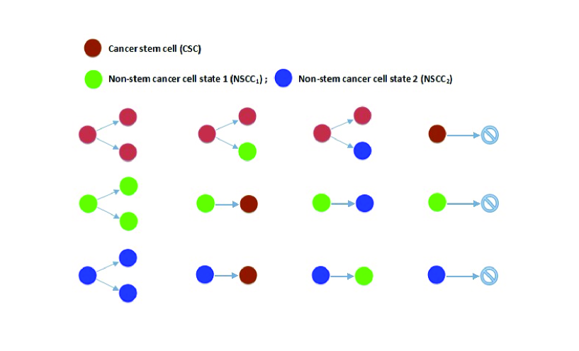
Figure 1: The model illustrated by the three-phenotype example (CSC, $\textrm{NSCC}_{1}$, $\textrm{NSCC}_{2}$). For CSC (first row, left to right): symmetric division, asymmetric division (differentiation to $\textrm{NSCC}_{1}$), asymmetric division (differentiation to $\textrm{NSCC}_{2}$), and cell death; For $\textrm{NSCC}_{1}$ (second row, left to right): symmetric division, phenotypic conversion to CSC, phenotypic conversion to $\textrm{NSCC}_{2}$, and cell death; For $\textrm{NSCC}_{2}$ (third row, left to right): symmetric division, phenotypic conversion to CSC, phenotypic conversion to $\textrm{NSCC}_{1}$, and cell death.

We list the elements of the model in table 1 (see Fig. 1 for the example of three phenotypes). If we denote $X^{0}_{t}$, $X^{1}_{t}$,…, $X^{m}_{t}$ as the cell numbers of CSC, $\textrm{NSCC}_{1}$, …, $\textrm{NSCC}_{m}$ at time $t$ respectively, then $\overrightarrow{X_{t}}=(X^{0}_{t},X^{1}_{t},...,X^{m}_{t})^{T}$ is an ($m+1$)-dimensional cellular system consisting of $(m+1)\times(m+2)$ cellular processes. On the basis of the modeling principles in biochemical reactions (see Chapter 7 in [38]), our cellular system can be formulated by both stochastic and deterministic models as follows:

Table 1: Parameters used in the model

Symbol	Parameter	Cellular process
$\alpha_{00}$	symmetric division rate by CSC	CSC $\overset{\alpha_{00}}{\longrightarrow}$ CSC+CSC
$\alpha_{0j}$	asymmetric division rate by CSC	CSC $\overset{\alpha_{0j}}{\longrightarrow}$ CSC+$\textrm{NSCC}_{j}$ ($1\leq j\leq m$)
$\alpha_{0}$	death rate by CSC	CSC $\overset{\alpha_{0}}{\longrightarrow}$ $\emptyset$
$\alpha_{ii}$	symmetric division rate by $\textrm{NSCC}_{i}$	$\textrm{NSCC}_{i}$ $\overset{\alpha_{ii}}{\longrightarrow}$ $\textrm{NSCC}_{i}$+$\textrm{NSCC}_{i}$ ($1\leq i\leq m$)
$\alpha_{i0}$	phenotypic conversion rate from $\textrm{NSCC}_{i}$ to CSC	$\textrm{NSCC}_{i}$ $\overset{\alpha_{i0}}{\longrightarrow}$ CSC ($1\leq i\leq m$)
$\alpha_{ij}$	phenotypic conversion rate from $\textrm{NSCC}_{i}$ to $\textrm{NSCC}_{j}$	$\textrm{NSCC}_{i}$ $\overset{\alpha_{ij}}{\longrightarrow}$ $\textrm{NSCC}_{j}$ ($i\neq j$)
$\alpha_{i}$	death rate by $\textrm{NSCC}_{i}$	$\textrm{NSCC}_{i}$ $\overset{\alpha_{i}}{\longrightarrow}$ $\emptyset$ ($1\leq i\leq m$)

2.2 Stochastic model

The randomness of cellular systems is essentially rooted in the stochastic nature of gene expression in individual cells [39]. The emergence of determinism from randomness is a result of the Law of Large Numbers. In other words, when the population is not large enough and subject to stochastic fluctuations, $\overrightarrow{X}=(X^{0}_{t},X^{1}_{t},...,X^{m}_{t})^{T}$ should be stochastic. According to the theory of Chemical Master Equation (CME) (see Chapter 11 in [40]), the stochastic model can be formulated by a continuous-time Markov process on $\mathbb{N}^{m+1}$. If we define $\textrm{Pr}\{x_{0},...,x_{i},...,x_{m};t\}$ as the probability of $\overrightarrow{X}=(x_{0},...,x_{i},...,x_{m})^{T}$ at time $t$, then the rate of change in $\textrm{Pr}\{x_{0},...,x_{i},...,x_{m};t\}$ is equal to the rate of transition from all the other possible states to $(x_{0},...,x_{i},...,x_{m})$ minus the rate of transition from $(x_{0},...,x_{i},...,x_{m})$ to all the other possible states, formally,

$$\frac{d\textrm{Pr}\{x_{0},...,x_{i},...,x_{m};t\}}{dt}=F(x_{0},...,x_{i},...,x_{m},t),$$ (1)

where

$$F(x_{0},...,x_{i},...,x_{m},t) = \sum_{i=0}^{m}(x_{i}-1)\alpha_{ii}\textrm{Pr}\{x_{0},...,x_{i}-1,...,x_{m};t\}$$

$$+\sum_{i=0}^{m}(x_{i}+1)\alpha_{i}\textrm{Pr}\{x_{0},...,x_{i}+1,...,x_{m};t\}$$

$$+\sum_{j=1}^{m}(x_{0}\alpha_{0j}\textrm{Pr}\{x_{0},...,x_{j}-1,...,x_{m};t\})$$

$$+\sum_{\begin{subarray}{c}(i,j)\in\{1,2,...,m\}\times\{0,1,...,m\}\\ \textrm{with}~{}i\neq j\end{subarray}}(x_{i}+1)\alpha_{ij}\textrm{Pr}\{x_{0},...,x_{i}+1,...,x_{j}-1...,x_{m};t\}$$

$$-\sum_{(i,j)\in\{0,1,...,m\}\times\{0,1,...,m\}}(x_{i}\alpha_{ij})\textrm{Pr}\{x_{0},...,x_{i},...,x_{m};t\}$$

$$-\sum_{i=0}^{m}(x_{i}\alpha_{i})\textrm{Pr}\{x_{0},...,x_{i},...,x_{m};t\}.$$

The first four items of $F(x_{0},...,x_{i},...,x_{m},t)$ describe the transitions from other states to $(x_{0},...,x_{i},...,x_{m})$. For example, the first item corresponds to the sum of the rates of transition from $(x_{0},...,x_{i}-1,...,x_{m})$ to $(x_{0},...,x_{i},...,x_{m})$ by symmetric division of $i^{th}$ cell phenotype, $0\leq i\leq m$. Similarly, the other three items can be explained by other types of cellular processes accordingly. The last two items of $F(x_{0},...,x_{i},...,x_{m},t)$ describe the transitions from $(x_{0},...,x_{i},...,x_{m})$ to other states. Since it is difficult to calculate the analytic solution of $\textrm{Pr}\{x_{0},...,x_{i},...,x_{m};t\}$, stochastic simulation (called Gillespie algorithm [41]) can often be used as an efficient numerical approach to investigate the CME.

When the population size is large enough, it is more convenient to use deterministic equations to capture the model:

2.3 Deterministic model

Let $\langle\overrightarrow{X_{t}}\rangle=(\langle X^{0}_{t}\rangle,\langle X^{1}_{t}\rangle,...,\langle X^{m}_{t}\rangle)^{T}$ be the expectation of $\overrightarrow{X_{t}}$, where

$$\langle X^{i}_{t}\rangle:=\sum_{x_{0},...,x_{i},...,x_{m}}x_{i}\textrm{Pr}\{x_{0},...,x_{i},...,x_{m};t\}~{}~{}(0\leq i\leq m).$$

We now derive the equation governing the dynamics of $\langle X^{i}_{t}\rangle$ (our method is based on Section 5.8 in [38]). We multiply $x_{i}$ on the both sides of (1), and then calculate the summation over all the indexes

$$\sum_{x_{0},...,x_{i},...,x_{m}}(x_{i}\frac{d\textrm{Pr}\{x_{0},...,x_{i},...,x_{m};t\}}{dt})=\sum_{x_{0},...,x_{i},...,x_{m}}(x_{i}F(x_{0},...,x_{i},...,x_{m},t)),$$

that is,

$$\frac{d\langle X^{i}_{t}\rangle}{dt}=\sum_{x_{0},...,x_{i},...,x_{m}}(x_{i}F(x_{0},...,x_{i},...,x_{m},t)).$$

Then we have
1) when $i=0$

$$\frac{d\langle X^{0}_{t}\rangle}{dt}=(\alpha_{00}-\alpha_{0})\langle X^{0}_{t}\rangle+\sum_{i=1}^{m}(\alpha_{i0}\langle X^{i}_{t}\rangle)).$$ (2)

2) when $1\leq i\leq m$

$$\frac{d\langle X^{i}_{t}\rangle}{dt}=\sum_{j\neq i}\alpha_{ji}\langle X^{j}_{t}\rangle+(\alpha_{ii}-\alpha_{i}-\sum_{j\neq i}\alpha_{ij})\langle X^{i}_{t}\rangle.$$ (3)

Thus the dynamics of $\langle\overrightarrow{X_{t}}\rangle$ can be formulated by the following $(m+1)$-dimensional linear ordinary differential equations (ODEs)

$$\frac{d\langle\overrightarrow{X_{t}}\rangle}{dt}=A\langle\overrightarrow{X_{t}}\rangle,$$ (4)

where

$$A=\left(\begin{smallmatrix}\alpha_{00}-\alpha_{0}&\alpha_{10}&\alpha_{20}&\cdots&\alpha_{m0}\\ \alpha_{01}&\alpha_{11}-\alpha_{1}-\sum_{j\neq 1}\alpha_{1j}&\alpha_{21}&\cdots&\alpha_{m1}\\ \vdots&\vdots&\vdots&\vdots&\vdots\\ \alpha_{0(m-1)}&\cdots&\cdots&\alpha_{(m-1)(m-1)}-\alpha_{(m-1)}-\sum_{j\neq(m-1)}\alpha_{(m-1)j}&\alpha_{m(m-1)}\\ \alpha_{0m}&\cdots&\cdots&\alpha_{(m-1)m}&\alpha_{mm}-\alpha_{m}-\sum_{j\neq m}\alpha_{mj}\\ \end{smallmatrix}\right).$$ (5)

It is noteworthy that Eq. (4) can also be obtained based on the Law of Mass Action (LMA) [42], indicating the equivalent kinetic foundation between the stochastic theory of CME and its deterministic counterpart of LMA. If we choose to ignore cancer cell plasticity in the model, i.e. let $\alpha_{ij}=0$ $(1\leq i\leq m,0\leq j\leq m$, and $i\neq j)$, the form of $A$ will reduce to the one governing the hierarchical cancer stem cell model:

$$A^{*}=\left(\begin{array}[]{ccccc}\alpha_{00}-\alpha_{0}&0&0&\cdots&0\\ \alpha_{01}&\alpha_{11}-\alpha_{1}&0&\cdots&0\\ \vdots&\vdots&\vdots&\vdots&\vdots\\ \alpha_{0(m-1)}&\cdots&\cdots&\alpha_{(m-1)(m-1)}-\alpha_{(m-1)}&0\\ \alpha_{0m}&\cdots&\cdots&0&\alpha_{mm}-\alpha_{m}\\ \end{array}\right).$$ (6)

In comparison of $A$ and $A^{*}$, it is interesting that there seems to be a trade-off between the diagonal and off-diagonal elements, that is, $A$ has larger off-diagonal elements but smaller diagonal elements than $A^{*}$. Note that the diagonal elements correspond to the growth contributions from the cells with the same phenotypes themselves while the off-diagonal elements are the contributions from other phenotypes, cancer cell plasticity can be interpreted as a altruism behavior among cancer cells in the sense that it makes cancer cells of one phenotype help other phenotypes to survive by sacrificing their own phenotype [43]. How this altruism behavior affects the population structure of cancer cells is one of the major tasks in the study of cell plasticity models.

In the following two sections, we will analyze both the asymptotic and transient dynamics of the model, then apply the theoretical results to explain the problems arising from concrete biological experiments.

3 Phenotypic equilibrium and frequency model

It has been reported in various cancer cell lines [17, 20, 21, 30] that, the cancer cell populations starting from different initial proportions can return towards equilibrium proportions over time. The arise of this phenotypic equilibrium has performed as a profound indication in support of the intrinsic homeostasis in cancer. To explain this phenomenon, we investigate the dynamics of phenotypic proportions in this section.

The model in previous section describes the population dynamics of the absolute cell numbers of different phenotypes. However in reality, relative numbers, i.e. the proportions of cell phenotypes are usually measured by fluorescence-activated cell sorting (FACS) experiments. Thus one often converts the population model to a frequency model.

Let $N_{t}$ be the total number of the population, $N_{t}=X^{0}_{t}+X^{1}_{t}+...+X^{m}_{t}$, the proportion of $X^{i}_{t}$ is defined as $x^{i}_{t}=X^{i}_{t}/N_{t}.$ Then $\overrightarrow{x_{t}}=(x^{0}_{t},x^{1}_{t},...,x^{m}_{t})^{T}$ is the vector describing the phenotypic proportions. Let $\langle\overrightarrow{x_{t}}\rangle$ be the expectation of $\overrightarrow{x_{t}}$, from Eq. (4) we can obtain the nonlinear (second order) ODEs governing the dynamics of $\langle\overrightarrow{x_{t}}\rangle$ as follows (see mathematical details in 6.1):

$$\frac{d\langle\overrightarrow{x_{t}}\rangle}{dt}=A\langle\overrightarrow{x_{t}}\rangle-\langle\overrightarrow{x_{t}}\rangle e^{T}A\langle\overrightarrow{x_{t}}\rangle,$$ (7)

where $e=(1,1,...,1)^{T}.$ Note that $x^{0}_{t}+x^{1}_{t}+...+x^{m}_{t}=1$, if replacing $x^{m}_{t}$ by $1-(x^{0}_{t}+x^{1}_{t}...+x^{m-1}_{t})$, the dimension of Eq. (7) should reduce from $m+1$ to $m$ (see 6.1).

To show the stability of the frequency model Eq. (7), we have Theorem 1:

Theorem 1

If the Perron-Frobenius eigenvalue $\lambda_{1}$ of the matrix $A$ in Eq. (5) is simple (i.e. the algebraic multiplicity of $\lambda_{1}$ is equal to one), then Eq. (7) has one and only one stable fixed point and no stable limit cycle.
(Technically, in very few cases it is necessary to add a small perturbation to the initial state for completing the final proof, see proof in 6.2)

The Perron-Frobenius eigenvalue $\lambda_{1}$ is the largest real eigenvalue satisfying that Re$\lambda<\lambda_{1}$ for every other $\lambda$ (6.2). On account of the inevitability of perturbations in real world, it can be proved that almost surely the algebraic multiplicity of $\lambda_{1}$ is equal to one (6.3). Especially when validating the model with biological experiments, the condition of Theorem 1 can easily be satisfied. Theorem 1 thus theoretically explains the phenotypic equilibrium phenomena observed in cancer cell lines, that is, starting from different initial proportions, the cancer cell population can return towards stable equilibrium proportions as time passes. Furthermore, note that Theorem 1 holds for the general cases with any finite phenotypes, it can be predicted that the phenotypic equilibrium should be universal in multi-phenotypic population of cancer cells.

In next section we will turn our attention from long-term asymptotic behavior to transient dynamics of the model.

4 Transient analysis and cell plasticity

In this section, we investigate how the cell plasticity influences the transient proportions of cell phenotypes and maintains the heterogeneity of cancer.

To explore the proportion of any phenotype $i$ ($0\leq i\leq m$), from Eq. (7) we have

$$\frac{d\langle x^{i}_{t}\rangle}{dt}=\sum_{j=0}^{m}(a_{ij}\langle x^{j}_{t}\rangle)-\langle x^{i}_{t}\rangle\sum_{n=0}^{m}\sum_{j=0}^{m}(a_{nj}\langle x^{j}_{t}\rangle).$$ (8)

We are interested in how $\langle x^{i}_{t}\rangle$ changes shortly after the drastic reduction of it. This problem is of particular interest to cancer biologists because of two major lines: One is that in cell culture experiments, they care about the transient changes of cancer cells shortly after the cell sorting. The other is that they are concerned about how the residual cancer cells relapse after the treatments.

Assume that the proportion of phenotype $i$ at time $t_{0}$ becomes very small, i.e. $\langle x^{i}_{t_{0}}\rangle\approx 0$. Then Eq. (8) can be approximately simplified as follows

$$\left.\frac{d\langle x^{i}_{t}\rangle}{dt}\right|_{t=t_{0}}\approx\sum_{j\neq i}^{m}(a_{ij}\langle x^{j}_{t_{0}}\rangle).$$ (9)

Eq. (9) indicates that the transient growth of $\langle x^{i}_{t}\rangle$ at time $t_{0}$ is almost contributed by the cell-state conversions from other phenotypes provided that current proportion of phenotype $i$ is very small. That is, as soon as the cancer cells of one phenotype dramatically decreases, cancer cell plasticity helps increase their phenotypic proportion, which serves as a mutual-helping mechanism in transient dynamics. In particular, suppose the great majority of CSCs have already been eliminated (e.g. by CSCs-targeted drugs or cell sorting), i.e. $\langle x^{0}_{t_{0}}\rangle\approx 0$. It is easy to distinguish the conventional CSC model from the one with cell plasticity by comparing their transient dynamics: In conventional CSC model without cancer cell plasticity, the growth of CSCs relies only on the self-renewal of CSCs themselves, the initial growth of CSCs proportion should be very limited (constrained by the rate limitation of cell division cycle); In contrast, the de-differentiations from other NSCCs can effectively speed up the transient grow rate of CSCs proportion. In this way, there should be a disparity of the transient increase between these two models shortly after the initial time $t_{0}$. To further illustrate the impact of cell plasticity on transient change of CSCs proportion, we will discuss two concrete examples in next two subsections: CSC-NSCC model and S-B-L model.

4.1 CSC-NSCC model

CSC-NSCC model is the most widely studied cell plasticity model. In this model, besides CSCs, all the other non-CSCs are grouped into one whole phenotype. We now treat the CSC-NSCC model as a two-phenotypic example of the multi-phenotypic framework, which contains six cellular processes as follows:
1) CSC $\overset{\alpha_{00}}{\longrightarrow}$ CSC+CSC;
2) CSC $\overset{\alpha_{01}}{\longrightarrow}$ CSC+NSCC;
3) CSC $\overset{\alpha_{0}}{\longrightarrow}$ $\emptyset$.
4) NSCC $\overset{\alpha_{10}}{\longrightarrow}$ CSC.
5) NSCC $\overset{\alpha_{11}}{\longrightarrow}$ NSCC+NSCC;
6) NSCC $\overset{\alpha_{1}}{\longrightarrow}$ $\emptyset$;

Let $s_{t}$ be CSCs proportion, and $n_{t}=1-s_{t}$ be NSCCs proportion, the equation governing the change of CSCs proportion is then given by

$$\frac{d\langle s_{t}\rangle}{dt}=-C\langle s_{t}\rangle^{2}+D\langle s_{t}\rangle+\alpha_{10},$$ (10)

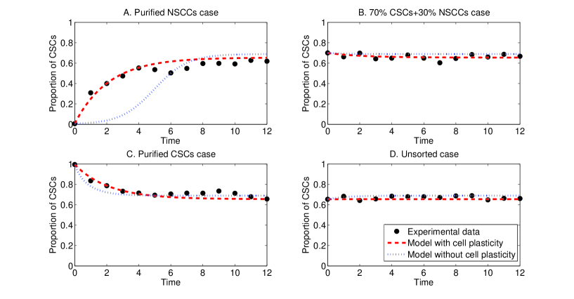
Figure 2: The comparison of CSC-NSCC models (10) with and without cell plasticity by fitting to experimental data on SW620 colon cancer cell line: The black dots are the experimental data in [20], the blue dashed lines are the predictions of the model without cell plasticity ($\alpha_{10}=0$), and the red dashed lines are the predictions of the model with cell plasticity ($\alpha_{10}>0$). There are four groups of data in the experiment: A) Purified NSCCs case ($0.6\%$ CSCs+$99.4\%$ NCSSs); B) $70\%$ CSCs+$30\%$ NCSSs; C) Unsorted case ($65.4\%$ CSCs+$34.6\%$ NCSSs); D) Purified CSCs case ($99.4\%$ CSCs+$0.6\%$ NCSSs). By least squares method, we predicted the values of four different cases together with the best fitting parameters (see methods in 6.4). It is shown that in (B), (C) and (D), the predicted trajectories by both models are in good accord with the data. In (A), however, compared to the sigmoidal growth pattern predicted by the model without cell plasticity, the prediction by the model with cell plasticity shows a transient increase in the first few days, which is in line with the experimental data.

where $C=(\alpha_{00}+\alpha_{01}-\alpha_{0})-(\alpha_{11}-\alpha_{1})$ and $D=(\alpha_{00}-\alpha_{0})-(\alpha_{11}+\alpha_{10}-\alpha_{1})$. Note that $\alpha_{10}$ is the transition rate from NSCCs to CSCs, the model will reduce to the conventional CSC model without cell plasticity by letting $\alpha_{10}=0$. Fig. 2 shows the comparison of the models with and without cell plasticity by validating them to the published data on SW620 colon cancer cell line [20]. The method for parameter fitting we performed is presented in 6.4. It is found that the major difference between the two models lies in purified NSCCs case (Fig. 2A): Starting from very small CSCs proportion ($0.6\%$ purity), the initial growth of CSCs proportion predicted by the model without cell plasticity is very slow, the growth rate will gradually increase until CSCs proportion tends to its equilibrium level, which shows a typical sigmoidal growth pattern [44]. However, the model with cell plasticity predicted a transient increase of CSCs proportion shortly after the initiation, which is in line with the experimental data. Even though both models predict the final phenotypic equilibrium, only can the model with cell plasticity fit the transient change on the data. This indicates that cancer cell plasticity could play more essential role in transient dynamics than in long-term behavior of CSCs proportion. A similar result is obtained if the stochastic version of the model is simulated using Gillespie algorithm (see 6.5).

4.2 S-B-L model

We now consider a three-phenotypic example of our model. Enlightened by Gupta et al.’s work [21], the three-phenotypic model comprises of stem-like (S), basal (B) and luminal cells (L). Based on our framework, S-B-L model contains twelve reactions as follows:
1) S $\overset{\alpha_{00}}{\longrightarrow}$ S+S;
2) S $\overset{\alpha_{01}}{\longrightarrow}$ S+B;
3) S $\overset{\alpha_{02}}{\longrightarrow}$ S+L;
4) S $\overset{\alpha_{0}}{\longrightarrow}$ $\emptyset$.
5) B $\overset{\alpha_{11}}{\longrightarrow}$ B+B;
6) B $\overset{\alpha_{10}}{\longrightarrow}$ S;
7) B $\overset{\alpha_{12}}{\longrightarrow}$ L;
8) B $\overset{\alpha_{1}}{\longrightarrow}$ $\emptyset$;
9) L $\overset{\alpha_{22}}{\longrightarrow}$ L+L;
10) L $\overset{\alpha_{20}}{\longrightarrow}$ S;
11) L $\overset{\alpha_{21}}{\longrightarrow}$ B.
12) L $\overset{\alpha_{2}}{\longrightarrow}$ $\emptyset$;

Let $(s_{t},b_{t},l_{t})^{T}$ be the vector describing the proportions of (S, B, L), then we have

$$\left\{\begin{aligned} \frac{d\langle s_{t}\rangle}{dt}&=(\alpha_{00}-\alpha_{0})\langle s_{t}\rangle+\alpha_{10}\langle b_{t}\rangle+\alpha_{20}\langle l_{t}\rangle-s_{t}[A_{1}\langle s_{t}\rangle+A_{2}\langle b_{t}\rangle+A_{3}\langle l_{t}\rangle]\\ \frac{d\langle b_{t}\rangle}{dt}&=\alpha_{01}\langle s_{t}\rangle+(\alpha_{11}-\alpha_{10}-\alpha_{12}-\alpha_{1})\langle b_{t}\rangle+\alpha_{21}\langle l_{t}\rangle-\langle b_{t}\rangle[A_{1}\langle s_{t}\rangle+A_{2}\langle b_{t}\rangle+A_{3}\langle l_{t}\rangle]\\ \frac{d\langle l_{t}\rangle}{dt}&=\alpha_{02}\langle s_{t}\rangle+\alpha_{12}\langle b_{t}\rangle+(\alpha_{22}-\alpha_{20}-\alpha_{21}-\alpha_{2})\langle l_{t}\rangle-\langle l_{t}\rangle[A_{1}\langle s_{t}\rangle+A_{2}\langle b_{t}\rangle+A_{3}\langle l_{t}\rangle]\\ \end{aligned}\right.$$ (11)

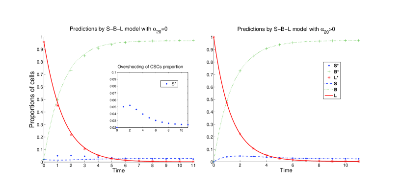
Figure 3: Predictions of S-B-L model: We fitted Eq. (11) to the cell-state dynamics on the data of SUM159 breast cancer cell line (Figure 3 in [21]). $S$, $B$ and $L$ are the predictions by the model, while $S^{*}$, $B^{*}$ and $L^{*}$ are the cell-state dynamics on data. There are three groups of data: A) Purified stem-like cells case; B) Purified basal cells case; C) Purified luminal cells case. We predicted the time points of three different cases together with the best fitting parameters. This figure shows the predictions in purified luminal case, see 6.4 for the other two cases. The left panel is the predictions by the model without phenotypic conversion from luminal cells to stem-like cells ($\alpha_{20}=0$), while the right panel is the predictions by the model with phenotypic conversion from luminal cells to stem-like cells ($\alpha_{20}>0$). It is shown that only can the model with cell plasticity predict the overshooting of the proportion of stem-like cells. The small window in left panel specifically focuses on the overshooting phenomenon of stem-like cells.

where $A_{1}=\alpha_{00}+\alpha_{01}+\alpha_{02}-\alpha_{0}$, $A_{2}=\alpha_{11}-\alpha_{1}$, $A_{3}=\alpha_{22}-\alpha_{2}$. Fig. 3 shows the predictions of S-B-L model by fitting to cell-state dynamics on data of SUM159 breast cancer cell line [21](see methods in 6.4). Starting from very small $\langle s_{0}\rangle$, in contrast to the gradual increase of $\langle s_{t}\rangle$ predicted by the model with $\alpha_{20}=0$, there is an overshooting of $\langle s_{t}\rangle$ predicted by the model with $\alpha_{20}>0$, which is in line with the cell-state dynamics observed in experiment. That is, the proportion of stem-like cells is rapidly elevated by de-differentiation to the value above the equilibrium level, and then returns towards the final equilibrium as time passes. It has been reported that CSC-NSCC model can never perform overshooting [27, 45], which implies that the overshooting phenomenon are rooted in the diversity of phenotype in the multi-phenotypic model. Moreover, note that overshooting behavior is a result of biological response to environmental stimulus through evolution [46], cancer cell plasticity may have meaningful implications for the evolution of cancer. One possible explanation is that the reversible phenotype switching between cells provides an advantageous cooperative strategy for cancer cell populations during their competitions with various anticancer mechanisms [43], thus increases their collective fitness. This idea is in line with the literature in ecology and population genetics [32, 34] regarding phenotypic variability as a surviving strategy for biological populations in fluctuating environments.

5 Conclusions

Instead of the hierarchical structure of cancer cells proposed by cancer stem cell theory, the updated CSC paradigm with cell plasticity suggests a reversible nature between different cancer cell phenotypes. In this study we proposed a generalized multi-phenotypic cancer model for providing a mathematical framework to investigate the interplay between cell plasticity and diversity of phenotypes in cancer. Based on our model, some interesting and insightful results have been achieved. On one hand, it was shown (in Theorem 1) that the phenotypic equilibrium phenomena can be predicted by the stability of our frequency model. On the other hand, by comparing the models with and without cell plasticity, it was found that cell plasticity may play more essential role in transient dynamics. It has been shown that only can the models with cell plasticity predict the transient increase and overshooting phenomena in CSCs proportion. In particular, the overshooting phenomenon performed by the S-B-L model was shown to be one of the salient features in the multi-phenotypic models with cell plasticity. With the further study of the multi-phenotypic models with cell plasticity, more interesting and insightful phenomena would be found in future.

Cancer cell plasticity has enriched the theory of cancer stem cell and comes along with new fundamental problems in cancer biology: Firstly, its molecular mechanism is poorly understood. It was reported that TGF-$\beta$ might have important roles in the process of cell-state conversions through activating epithelial mesenchymal transition (EMT) [20]. Further studies on related molecular models should be important tasks. Accordingly, besides the population-level models studied in this work, molecular-level models should also be accounted for in future. Secondly, even though cell plasticity is found to be intimately related to the heterogeneity of cancer, cancer complexity is a result of multifactorial mechanisms (e.g. clonal evolution, tumor microenvironment, reversible cell plasticity and etc [47]), and it is not clear in which cancer and to what extent the disease progression arises from the cell plasticity. That is, how to distinguish cell plasticity from other sources of cancer heterogeneity should be a central problem in future, for both theoretical and experimental researchers.

6 Appendix

6.1 Derivation of Eq. (7)

For Eq. (4)

$$\frac{d\langle X^{i}_{t}\rangle}{dt}=a_{i0}\langle X^{0}_{t}\rangle+a_{i1}\langle X^{1}_{t}\rangle+...+a_{im}\langle X^{m}_{t}\rangle.$$

Note that

$$x^{i}_{t}=\frac{X^{i}_{t}}{X^{0}_{t}+X^{1}_{t}+...+X^{m}_{t}}=\frac{X^{i}_{t}}{N_{t}},$$

$$\frac{d\langle X^{i}_{t}\rangle}{dt}=\frac{d(\langle x^{i}_{t}\rangle\langle N_{t}\rangle)}{dt}=\langle x^{i}_{t}\rangle\frac{d}{dt}\langle N_{t}\rangle+\langle N_{t}\rangle\frac{d\langle x^{i}_{t}\rangle}{dt},$$

then

$$\frac{d\langle x^{i}_{t}\rangle}{dt} =\frac{1}{\langle N_{t}\rangle}\frac{d\langle X^{i}_{t}\rangle}{dt}-\frac{\langle x^{i}_{t}\rangle}{\langle N_{t}\rangle}\frac{d\langle N_{t}\rangle}{dt}$$

$$=\sum_{j=0}^{m}(a_{ij}\langle x^{j}_{t}\rangle)-\langle x^{i}_{t}\rangle\sum_{n=0}^{m}\sum_{j=0}^{m}(a_{nj}\langle x^{j}_{t}\rangle).$$

Then we have Eq. (7).

By letting $x^{m}_{t}=1-(x^{0}_{t}+x^{1}_{t}...+x^{m-1}_{t})$, we have (for $0\leq i\leq m-1$)

$$\frac{d\langle x^{i}_{t}\rangle}{dt} =\sum_{j=0}^{m}(a_{ij}\langle x^{j}_{t}\rangle)-\langle x^{i}_{t}\rangle\sum_{n=0}^{m}\sum_{j=0}^{m}(a_{nj}\langle x^{j}_{t}\rangle)$$

$$=\sum_{j=0}^{m-1}(a_{ij}\langle x^{j}_{t}\rangle)+a_{im}\langle x^{m}_{t}\rangle-\langle x^{i}_{t}\rangle\sum_{n=0}^{m}\left(\sum_{j=0}^{m-1}(a_{nj}\langle x^{j}_{t}\rangle)+a_{nm}\langle x^{m}_{t}\rangle\right)$$

$$=\sum_{j=0}^{m-1}(a_{ij}-a_{im})\langle x^{j}_{t}\rangle-\langle x^{i}_{t}\rangle\sum_{n=0}^{m}\left(\sum_{j=0}^{m-1}(a_{nj}-a_{nm})\langle x^{j}_{t}\rangle+a_{nm}\right)+a_{im}$$

$$=\underbrace{-\langle x^{i}_{t}\rangle\sum_{n=0}^{m}\sum_{j=0}^{m-1}(a_{nj}-a_{nm})\langle x^{j}_{t}\rangle}_{\textrm{nonlinear term}}\underbrace{-\langle x^{i}_{t}\rangle\sum_{n=0}^{m}a_{nm}+\sum_{j=0}^{m-1}(a_{ij}-a_{im})\langle x^{j}_{t}\rangle}_{\textrm{linear term}}\underbrace{+a_{im}.}_{\textrm{constant term}}$$

6.2 Proof of Theorem 1

Let us first consider the properties of Eq. (4). We will show that there exists a largest real eigenvalue $\lambda_{1}$ of $A$ satisfying Re$\lambda<\lambda_{1}$ for every other $\lambda$. Note that the off-diagonal elements of the matrix $A$ are non-negative, $A+\kappa I$ becomes a non-negative matrix ($I$ is the identity matrix) when $\kappa$ is large enough. By Perron-Frobenius theory (see chapter 1 in [48]), $A+\kappa I$ has an real eigenvalue $\lambda^{\prime}_{1}$ satisfying $Re\lambda^{\prime}<\lambda^{\prime}_{1}$ for any other eigenvalue $\lambda^{\prime}$ of $A+\kappa I$. It is easy to show that $\lambda^{\prime}_{1}-\kappa$ is just the largest real eigenvalue (called Perron-Frobenius eigenvalue $\lambda_{1}$) satisfying that Re$\lambda<\lambda_{1}$ for every other $\lambda$ of $A$ .

Suppose $\lambda_{1}$ is simple, the solution of Eq. (4) can be expressed as

$$\begin{split}&\langle\overrightarrow{X_{t}}\rangle=c_{1,1}\vec{u}e^{\lambda_{1}t}+\sum_{j=2}^{n}\sum_{l=1}^{n_{j}}c_{j,l}\sum_{i=1}^{n_{j}}\vec{r^{j}_{l,i}}t^{i-1}e^{\lambda_{j}t},\end{split}$$

where $\lambda_{1},\lambda_{2},\cdots{}\lambda_{n}$ are the different eigenvalues of $A$, $n_{j}$ is the algebraic multiplicity of $\lambda_{j}$, $\vec{u}$ is the normalized (i.e. $u_{0}+u_{2}+...+u_{m}=1$) right eigenvector of $\lambda_{1}$, $\vec{r^{j}_{l,i}}$ is the corresponding eigenvector of $\lambda_{j}$, $c_{j,l}$ is a constant determined by initial values. Note that Re$\lambda_{i}<\lambda_{1}~{}(i\neq 1)$, when $c_{1,1}\neq{}0$,

$$\begin{split}&\frac{\langle\overrightarrow{X_{t}}\rangle}{c_{1,1}e^{\lambda_{1}t}}=\vec{u}+\sum_{j=2}^{n}\sum_{l=1}^{n_{j}}\frac{c_{j,l}}{c_{1,1}}\sum_{i=1}^{n_{j}}\vec{r^{j}_{l,i}}t^{i-1}e^{(\lambda_{j}-\lambda_{1})t}\rightarrow\vec{u}.\end{split}$$

Thus

$$\langle\overrightarrow{x_{t}}\rangle=\frac{\langle\overrightarrow{X_{t}}\rangle}{\langle N_{t}\rangle}=\frac{\overrightarrow{X_{t}}/c_{1,1}e^{\lambda_{1}t}}{\langle N_{t}\rangle/c_{1,1}e^{\lambda_{1}t}}\rightarrow\frac{\vec{u}}{u_{0}+u_{2}+...+u_{m}}$$

Since $\vec{u}$ has been normalized, $\langle\overrightarrow{x_{t}}\rangle$ will tend to $\vec{u}$ when $t\rightarrow{}+\infty{}$.

In the following we will handle the case of $c_{1,1}=0$. Let $t=0$, we get the linear equations of $c_{j,l}$:

$$\begin{split}&c_{1,1}\vec{u}+\sum_{j=2}^{n}\sum_{l=1}^{n_{j}}c_{j,l}\vec{r^{j}_{l,1}}=\langle\overrightarrow{X_{0}}\rangle^{T}\end{split}$$

Denote the coefficient matrix by $B=[\vec{u}\ \vec{r^{2}_{1,1}}\ \vec{r^{2}_{2,1}}\cdots\vec{r^{n}_{n_{n},1}}]$, and let $B^{*}$ be $B$ with its first column replaced by $\langle\overrightarrow{X_{0}}\rangle^{T}$. Notice that columns of $B$ are linear independent. Then from Cramer’s rule

$$\begin{split}&c_{1,1}=\frac{det|B^{*}|}{det|B|},\end{split}$$

When $c_{1,1}=0$, namely $det|B^{*}|=0$, we can find an $n$-dimensional vector $\vec{v}$ which is linear independent with the last $n-1$ columns of $B$. Actually, with a small perturbation $\varepsilon{}\vec{v}$ to $\langle\overrightarrow{X_{0}}\rangle^{T}$, all the columns of $B^{*}$ are linear independent, and $c_{1,1}\neq{}0$. Note that fluctuations are inevitable in real world, $c_{1,1}\neq 0$ always holds in reality.

6.3 The algebraic multiplicity of Perron-Frobenius eigenvalue

It was shown above that the Perron-Frobenius eigenvalue $\lambda_{1}$ being simple is essential for proving Theorem 1. Here we will show that this condition is easily satisfied in real world. In fact, a more general result can be obtained as follows:

Proposition 1

Denote $\mathbb{R}^{n\times n}$ as the space of $n\times n$ real square matrices, equipped with Lebesgue measure. Then its subset of the matrices with repeated eigenvalues has measure zero.

To prove this proposition, we need following lemma first.

Lemma 1

For any non-zero polynomial $f(x_{1},x_{2},\cdots,x_{m})$ $(m\geq 1)$, its zero set has measure $0$ (w. r. t. Lebesgue measure on $\mathbb{R}^{m}$).

Proof of Lemma 3: We use inductive method. For $m=1$, the polynomial has only finite roots, whose zero set has measure $0$. Assume we have proved the lemma for $m=k-1$. For $m=k$, let us take $f(x_{1},x_{2},\cdots,x_{k})$ as the polynomial of $(x_{2},\cdots,x_{k})$, then the coefficients can be regarded as polynomials of $x_{1}$. It is easy to see that at most finite $x_{1}\in\mathbb{R}$ can make all coefficients equal to $0$. Denote such set of $x_{1}$ by $S$, then $\{(x_{1},x_{2},\cdots,x_{k}|\ x_{1}\in S\}$ has measure $0$ in $\mathbb{R}^{k}$. For any fixed $x_{1}\notin S$, $f(x_{1},x_{2},\cdots,x_{k})$ is a non-zero polynomial of $(x_{2},\cdots,x_{k})$. From inductive assumption we know its zero set has measure $0$ in $\mathbb{R}^{k-1}$. By Fubini-Tonelli theorem, we know that $\{(x_{1},x_{2},\cdots,x_{k})|\ x_{1}\notin S,\ f(x_{1},x_{2},\cdots,x_{k})=0\}$ has measure $0$ in $\mathbb{R}^{k}$. Thus $\{(x_{1},x_{2},\cdots,x_{k})|\ f(x_{1},x_{2},\cdots,x_{k})=0\}$ has measure $0$ in $\mathbb{R}^{k}$.

Proof of Proposition 1: It is easy to show that for any square matrix in $\mathbb{R}^{n\times n}$, the coefficients of its characteristic polynomial are polynomials of matrix entries. Thus the discriminant of the characteristic polynomial is again a polynomial of matrix entries. Applying Lemma 3 to the discriminant of characteristic polynomial, we have that the zero set of the discriminant has measure zero. And then according to the fact that a polynomial has repeated root if and only if its discriminant is $0$ [49], the set of the matrices with repeated eigenvalues has measure zero. The proof is completed.

Proposition 1 implies that almost surely the Perron-Frobenius eigenvalue $\lambda_{1}$ should be simple. In particular, perturbations are inevitable in the real work, so $\lambda_{1}$ can easily be simple. To further illustrate this result, we consider a $3\times 3$ example:

$$A=\left(\begin{array}[]{ccc}3&2&3\\ 0&3&5\\ 0&0&2\\ \end{array}\right),$$ (12)

its eigenvalues are $\lambda_{1}=\lambda_{2}=3$, $\lambda_{3}=2$. In this case the Perron-Frobenius eigenvalue $\lambda_{1}$ is repeated. However, if adding perturbations to $A$, e.g.

$$A=\left(\begin{array}[]{ccc}3.23&2.19&3.22\\ 0&3.78&5.11\\ 0&0&2.31\\ \end{array}\right),$$ (13)

its eigenvalues become $\lambda_{1}=3.78$, $\lambda_{2}=3.23$, $\lambda_{3}=2.31$. In this way the Perron-Frobenius eigenvalue $\lambda_{1}$ become simple.

Since the perturbations from experimental measurements and natural fluctuations are inevitable in reality, the Perron-Frobenius eigenvalue $\lambda_{1}$ in $A$ is seldom to be repeated. For example, consider the S-B-L model in Sec 4.2, let $\alpha_{00}=0.34$, $\alpha_{01}=0.29$, $\alpha_{02}=0.34$, $\alpha_{0}=0.11$, $\alpha_{11}=0.43$, $\alpha_{10}=0.07$, $\alpha_{12}=0.13$, $\alpha_{1}=0.09$, $\alpha_{22}=0.36$, $\alpha_{20}=0.06$, $\alpha_{21}=0.17$, $\alpha_{2}=0.10$, then the matrix $A$ turns to

$$A=\left(\begin{array}[]{ccc}0.23&0.09&0.10\\ 0.29&0.14&0.06\\ 0.34&0.07&0.03\\ \end{array}\right).$$ (14)

The eigenvalues of $A$ are $\lambda_{1}=0.4391$, $\lambda_{2}=-0.0844$, $\lambda_{3}=0.0453$. The Perron-Frobenius eigenvalue $\lambda_{1}$ is simple.

6.4 Methods for parameter fitting

We used least squares method to estimate the parameters. Let $\vec{y}=(y_{0},...,y_{n})^{T}$ be the data on $n$ time points, $\vec{x}(\vec{\theta})=(x_{0},...,x_{n})^{T}$ be the discrete trajectory of the model with parameter vector $\vec{\theta}$. The best-fitting parameters are obtained by solving the following least squares problem

$$\min_{\vec{\theta}}\sum_{i=0}^{n}(x_{i}-y_{i})^{2}.$$

Specifically, we first discuss the parameter fitting of the CSC-NSCC model to the data on SW620 cell line [20]. There are four groups of data in their experiment, each group contains 13 time points (from day 0 to day 24, the data points were recorded every two days). That is, there are a total of $13\times 4=52$ time points. We estimated the parameters in Eq. (10) by fitting to these 52 data points of four groups all together. It should be noted that, based on population-level data measured by FACS experiment, only can we estimate the values of $C$, $D$ and $\alpha_{10}$ in Eq. (10), we cannot estimate all the $\alpha_{ij}$ or ${\alpha_{i}}$ individually. However, it is interesting that $\alpha_{10}$ is presented as an independent coefficient, so we can still compare the models with and without cell plasticity based on the population-level analysis. We list the main points for parameter fitting as follows:

1. Fit four groups data together: Let $y^{j}_{i}$ be the $i^{th}$ time point in $j^{th}$ groups, then we need to solve the following least squares problem

   $$\min_{(C,D,\alpha_{10})}\sum_{j=1}^{4}\sum_{i=0}^{12}(x^{j}_{i}-y^{j}_{i})^{2}.$$

2. Fixed initial states: We set the initial states of Eq. (10) are the same as those on data, that is, let $x^{j}_{0}=y^{j}_{0}$ $(1\leq j\leq 4)$.

3. Parameter range: Based on the rate limitation of human cell proliferation cycle [50], we assume that each cell requires at least one day to finish a cell cycle. To rescale the discrete time point to continuous time and note that the data was recorded every two days, we have $0\leq\alpha_{ij}\leq 2\log 2$. Meanwhile, for the non-extinction of the cell population, we assume that cell death rate is smaller than symmetric division rate, i.e. $0\leq\alpha_{i}<\alpha_{ii}\leq 2\log 2$.

We performed fmincon algorithm in Matlab to calculate optimal values of $(C^{*},D^{*},\alpha^{*}_{10})$. To test the uniqueness of the solutions, 100 different starting values of $(C^{0},D^{0},\alpha^{0}_{10})$ were uniformly selected on the basis of the above parameter range. It was shown that the values of $(C,D,\alpha_{10})$ converge to $C^{*}\sim(10^{-6},10^{-5})$, $D^{*}=-0.4002\pm 0.0001$, and $\alpha^{*}_{10}=0.2630\pm 0.0002$. For the goodness of fit, the coefficient of determination is used to measure how well the observations on data are predicted by the models, that is,

$$R^{2}=1-\frac{SS_{res}}{SS_{tot}}=1-\frac{0.0588}{0.9921}=0.9407,$$

where $SS_{res}$ is the sum of squared residuals and $SS_{tot}$ is the total sum of squares (proportional to the sample variance) of data. By letting $\alpha_{10}=0$, with the same numerical scheme we have $C^{*}=1.3865\pm 0.0002$, $D^{*}=0.9550\pm 0.0001$, and the coefficient of determination is

$$R^{2}=1-\frac{SS_{res}}{SS_{tot}}=1-\frac{0.5932}{0.9921}=0.4021.$$

Fig 2A shows that the disparity between the predictions by the two models mainly lies in the transient dynamics in purified NSCCs case, where only can the model with $\alpha_{10}>0$ predict the transient increase of CSCs proportion.

Now we discuss the parameter fitting of the S-B-L model. The time-series data we used is the cell-state dynamics on SUM159 breast cancer cell line (Figure 3 in [21] ). There were three cases in their experiments (purified stem-like cells case, purified basal cells case and purified luminal cells case). In each case, 12 time points were recorded for each cell phenotype. That is, a total of $3\times 12\times 3=108$ data points were recorded. Note that $s_{t}+b_{t}+l_{t}=1$, the effective number of the data is actually reduced to 72. By letting $l_{t}=1-s_{t}-b_{t}$, we have

$$\left\{\begin{aligned} \frac{d\langle s_{t}\rangle}{dt}&=A_{4}\langle s_{t}\rangle+\alpha_{10}\langle b_{t}\rangle+\alpha_{20}\langle l_{t}\rangle-s_{t}[A_{1}\langle s_{t}\rangle+A_{2}\langle b_{t}\rangle+A_{3}\langle l_{t}\rangle]\\ \frac{d\langle b_{t}\rangle}{dt}&=\alpha_{01}\langle s_{t}\rangle+A_{5}\langle b_{t}\rangle+\alpha_{21}\langle l_{t}\rangle-\langle b_{t}\rangle[A_{1}\langle s_{t}\rangle+A_{2}\langle b_{t}\rangle+A_{3}\langle l_{t}\rangle]\\ \langle l_{t}\rangle&=1-s_{t}-b_{t}\\ \end{aligned}\right.$$ (16)

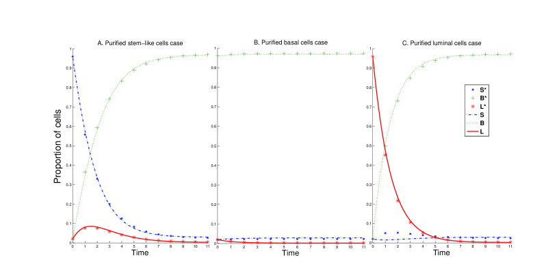
Figure 4: Fit Eq. (16) to cell-state dynamics in [21] by letting $\alpha_{20}=0$. The best fitting parameters are $A_{4}=0.032\pm 0.002$, $\alpha_{10}=0.016\pm 0.003$, $\alpha_{20}=0$, $A_{1}=0.578\pm 0.002$, $A_{2}=0.581\pm 0.002$, $A_{3}=0.550\pm 0.001$, $\alpha_{01}=0.416\pm 0.001$, $A_{5}=0.567\pm 0.002$ and $\alpha_{21}=0.693\pm 0.001$. The sum of squared residuals $SS_{res}$ are about 0.06 and the coefficient of determination $R^{2}=0.9851$. The unfitting part lies in the transient dynamics of the purified luminal cells case. In particular, the overshooting of the stem-like cells proportion cannot be predicted by the model.

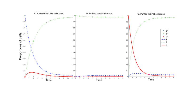
Figure 5: Fit Eq. (16) to cell-state dynamics in [21] by letting $\alpha_{20}>0$. The best fitting parameters are $A_{4}=0.027\pm 0.002$, $\alpha_{10}=0.013\pm 0.001$, $\alpha_{20}=0.071\pm 0.001$, $A_{1}=0.580\pm 0.002$, $A_{2}=0.578\pm 0.002$, $A_{3}=0.579\pm 0.001$, $\alpha_{01}=0.418\pm 0.001$, $A_{5}=0.567\pm 0.003$, and $\alpha_{21}=0.688\pm 0.001$. The sum of squared residuals is about $\sim(10^{-7},10^{-8})$, so the coefficient of determination $R^{2}$ is very close to 1.

where $A_{4}=\alpha_{00}-\alpha_{0}$, $A_{5}=\alpha_{11}-\alpha_{10}-\alpha_{12}-\alpha_{1}$. Similar to the CSC-NSCC model, on the basis of population level data, we cannot estimate all the twelve parameters $\alpha_{ij}$ and $\alpha_{i}$ in S-B-L model individually, since the freedom of the parameters in Eq. (16) is only nine. Note that the parameters for de-differentiation ($\alpha_{20}$ and $\alpha_{10}$) are presented as independent coefficients, it is feasible to investigate how de-differentiation influences the proportion of stem-like cells in transient dynamics. By applying similar numerical scheme we used in the CSC-NSCC model , we fitted Eq. (16) to the cell-state dynamics on data. Fig. 4 shows the predictions by the model with $\alpha_{20}=0$, and Fig. 5 shows the predictions by the model with $\alpha_{20}>0$. Note that the cell-state dynamic data in [21] was produced by the Markov chain, it is not surprising that the coefficients of determination of the two models are both close to 1. But it is note worthy that, the main difference between the two cases lies in the purified luminal case, where only can the model with $\alpha_{20}>0$ predict the overshooting of stem-like cells proportion.

6.5 Stochastic simulations

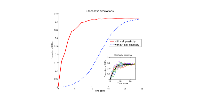
Figure 6: Stochastic simulation of CSC-NSCC model: It is shown that starting from very small CSCs proportion, the stochastic model without cell plasticity shows sigmoidal pattern growth, while the model with cell plasticity predicts the transient increase of CSCs proportion. This is in accord with the prediction by the Eq. (10) in Fig. 2A. The small window shows the strategy of our stochastic simulation. For given parameters, 20 stochastic samples (colorful thin lines) were produced by Monte carlo simulation. The thick black line is the representative trajectory by averaging these 20 stochastic samples.

The stochastic simulation of CSC-NSCC model is illustrated in Fig. 6. The simulation scheme we used is based on Monte Carlo simulation for the CME (see Section 11.4.4 in [40]).

6.6 A remark for the model

By adding symmetric differentiation of CSC into our model,

• CSC $\overset{\beta_{0j}}{\longrightarrow}$ $\textrm{NSCC}_{j}$+$\textrm{NSCC}_{j}$ ($1\leq j\leq m$)

the dynamics of $\langle\overrightarrow{X_{t}}\rangle$ can still be formed by the linear ODEs as follows

$$\frac{d\langle\overrightarrow{X_{t}}\rangle}{dt}=Q\langle\overrightarrow{X_{t}}\rangle,$$ (17)

where

$$Q=\left(\begin{smallmatrix}\alpha_{00}-\alpha_{0}-\sum_{j=1}^{m}\beta_{0j}&\alpha_{10}&\alpha_{20}&\cdots&\alpha_{m0}\\ \alpha_{01}+2\beta_{01}&\alpha_{11}-\alpha_{1}-\sum_{j\neq 1}\alpha_{1j}&\alpha_{21}&\cdots&\alpha_{m1}\\ \vdots&\vdots&\vdots&\vdots&\vdots\\ \alpha_{0(m-1)}+2\beta_{0(m-1)}&\cdots&\cdots&\alpha_{(m-1)(m-1)}-\alpha_{(m-1)}-\sum_{j\neq(m-1)}\alpha_{(m-1)j}&\alpha_{m(m-1)}\\ \alpha_{0m}+2\beta_{0m}&\cdots&\cdots&\alpha_{(m-1)m}&\alpha_{mm}-\alpha_{m}-\sum_{j\neq m}\alpha_{mj}\\ \end{smallmatrix}\right).$$ (18)

It is easy to find that the only difference between $Q$ and $A$ in Eq. (5) lies in the first column, but this does not change the non-negativity of the off-diagonal elements. Note that the main ingredient of the proof of Theorem 1 is the non-negativity of the off-diagonal elements in $A$ (see 6.2), Theorem 1 still holds for $Q$.

Moreover, the transient properties discussed in our model are still valid for the model with $Q$ here, by only replacing $a_{ij}$ in Eq. (8) with $q_{ij}$ here. Let us take the CSC-NSCC model as an example. The equation governing the change rate of CSCs proportion is given by

$$\frac{d\langle s_{t}\rangle}{dt}=-C^{*}\langle s_{t}\rangle^{2}+D^{*}\langle s_{t}\rangle+\alpha_{10},$$ (19)

where $C^{*}=(\alpha_{00}+\alpha_{01}+\beta_{01}-\alpha_{0})-(\alpha_{11}-\alpha_{1})$ and $D^{*}=(\alpha_{00}-\alpha_{0})-(\alpha_{11}+\alpha_{10}-\alpha_{1})$. the property of transient increase is still dependent on $\alpha_{10}$, which shares the same nature as Eq. (10).

Figures

References

- [1] T. Reya, S. Morrison, M. Clarke, I. Weissman, Stem cells, cancer, and cancer stem cells, Nature 414 (2001) 105–111.
- [2] C. Jordan, M. Guzman, M. Noble, Cancer stem cells, N. Engl. J. Med. 355 (12) (2006) 1253–1261.
- [3] P. Dalerba, R. Cho, M. Clarke, Cancer stem cells: models and concepts, Annu. Rev. Med. 58 (2007) 267–284.
- [4] C. Colijn, M. C. Mackey, A mathematical model of hematopoiesis i. periodic chronic myelogenous leukemia, J. Theor. Biol. 237 (2) (2005) 117–132.
- [5] M. D. Johnston, C. M. Edwards, W. F. Bodmer, P. K. Maini, S. J. Chapman, Mathematical modeling of cell population dynamics in the colonic crypt and in colorectal cancer, Proc. Natl. Acad. Sci. USA 104 (2007) 4008–4013.
- [6] B. Boman, M. Wicha, J. Fields, O. Runquist, Symmetric division of cancer stem cells–a key mechanism in tumor growth that should be targeted in future therapeutic approaches, Clin. Pharmacol. Ther. 81 (6) (2007) 893–898.
- [7] D. Dingli, A. Traulsen, F. Michor, (a) symmetric stem cell replication and cancer, PLoS Comput. Biol. 3 (3) (2007) e53.
- [8] M. D. Johnston, P. K. Maini, S. Jonathan Chapman, C. M. Edwards, W. F. Bodmer, On the proportion of cancer stem cells in a tumour, J. Theor. Biol. 266 (4) (2010) 708–711.
- [9] T. Antal, P. L. Krapivsky, Exact solution of a two-type branching process: models of tumor progression, J. Stat. Mech. 2011 (2011) P08018.
- [10] A. Sottoriva, L. Vermeulen, S. Tavaré, Modeling evolutionary dynamics of epigenetic mutations in hierarchically organized tumors, PLoS Comput. Biol. 7 (5) (2011) e1001132.
- [11] B. Werner, D. Dingli, T. Lenaerts, J. Pacheco, A. Traulsen, Dynamics of mutant cells in hierarchical organized tissues, PLoS Comput. Biol. 7 (12) (2011) e1002290.
- [12] T. Stiehl, A. Marciniak-Czochra, Mathematical modeling of leukemogenesis and cancer stem cell dynamics, Math. Model. Nat. Pheno. 7 (01) (2012) 166–202.
- [13] R. Molina-Peña, M. Álvarez, A simple mathematical model based on the cancer stem cell hypothesis suggests kinetic commonalities in solid tumor growth, PloS ONE 7 (2) (2012) e26233.
- [14] L. Nguyen, R. Vanner, P. Dirks, C. Eaves, Cancer stem cells: an evolving concept, Nat. Rev. Cancer 12 (2) (2012) 133–143.
- [15] J. Visvader, G. Lindeman, Cancer stem cells: current status and evolving complexities, Cell stem cell 10 (6) (2012) 717–728.
- [16] M. Meyer, J. Fleming, M. Ali, M. Pesesky, E. Ginsburg, B. Vonderhaar, Dynamic regulation of cd24 and the invasive, cd44poscd24neg phenotype in breast cancer cell lines, Breast Cancer Res. 11 (6) (2009) R82.
- [17] C. Chaffer, I. Brueckmann, C. Scheel, A. Kaestli, P. Wiggins, L. Rodrigues, M. Brooks, F. Reinhardt, Y. Su, K. Polyak, et al., Normal and neoplastic nonstem cells can spontaneously convert to a stem-like state, Proc. Natl. Acad. Sci. USA 108 (19) (2011) 7950–7955.
- [18] E. Quintana, M. Shackleton, H. R. Foster, D. R. Fullen, M. S. Sabel, T. M. Johnson, S. J. Morrison, Phenotypic heterogeneity among tumorigenic melanoma cells from patients that is reversible and not hierarchically organized, Cancer cell 18 (5) (2010) 510–523.
- [19] P. Scaffidi, T. Misteli, In vitro generation of human cells with cancer stem cell properties, Nat. Cell Biol. 13 (9) (2011) 1051–1061.
- [20] G. Yang, Y. Quan, W. Wang, Q. Fu, J. Wu, T. Mei, J. Li, Y. Tang, C. Luo, Q. Ouyang, et al., Dynamic equilibrium between cancer stem cells and non-stem cancer cells in human sw620 and mcf-7 cancer cell populations, Br. J. Cancer 106 (9) (2012) 1512–1519.
- [21] P. Gupta, C. Fillmore, G. Jiang, S. Shapira, K. Tao, C. Kuperwasser, E. Lander, Stochastic state transitions give rise to phenotypic equilibrium in populations of cancer cells, Cell 146 (4) (2011) 633–644.
- [22] R. French, R. Clarkson, The complex nature of breast cancer stem-like cells: Heterogeneity and plasticity, J. Stem Cell Res. Ther. S 7 (2012) 009.
- [23] A. O. Pisco, A. Brock, J. Zhou, A. Moor, M. Mojtahedi, D. Jackson, S. Huang, Non-darwinian dynamics in therapy-induced cancer drug resistance, Nat. Commun. 4 (2013) 2467.
- [24] S. Zapperi, C. La Porta, Do cancer cells undergo phenotypic switching? the case for imperfect cancer stem cell markers, Sci. Rep. 2 (2012) 441.
- [25] R. V. dos Santos, L. M. da Silva, A possible explanation for the variable frequencies of cancer stem cells in tumors, PloS one 8 (8) (2013) e69131.
- [26] R. V. dos Santos, L. M. da Silva, The noise and the kiss in the cancer stem cells niche, J. Theor. Biol. 335 (21) (2013) 79–87.
- [27] D. Zhou, D. Wu, Z. Li, M. Qian, M. Q. Zhang, Population dynamics of cancer cells with cell state conversions, Quant. Biol. 1 (3) (2013) 201–208.
- [28] W. Wang, Y. Quan, Q. Fu, Y. Liu, Y. Liang, J. Wu, G. Yang, C. Luo, Q. Ouyang, Y. Wang, Dynamics between cancer cell subpopulations reveals a model coordinating with both hierarchical and stochastic concepts, PloS one 9 (1) (2014) e84654.
- [29] K. Leder, K. Pitter, Q. LaPlant, D. Hambardzumyan, B. D. Ross, T. A. Chan, E. C. Holland, F. Michor, Mathematical modeling of pdgf-driven glioblastoma reveals optimized radiation dosing schedules, Cell 156 (3) (2014) 603–616.
- [30] D. Iliopoulos, H. Hirsch, G. Wang, K. Struhl, Inducible formation of breast cancer stem cells and their dynamic equilibrium with non-stem cancer cells via il6 secretion, Proc. Natl. Acad. Sci. USA 108 (4) (2011) 1397–1402.
- [31] D. M. Wolf, V. V. Vazirani, A. P. Arkin, Diversity in times of adversity: probabilistic strategies in microbial survival games, J. Theor. Biol. 234 (2) (2005) 227–253.
- [32] E. Kussell, S. Leibler, Phenotypic diversity, population growth, and information in fluctuating environments, Science 309 (5743) (2005) 2075–2078.
- [33] T. Lu, T. Shen, M. R. Bennett, P. G. Wolynes, J. Hasty, Phenotypic variability of growing cellular populations, Proc. Natl. Acad. Sci. USA 104 (48) (2007) 18982–18987.
- [34] M. Acar, J. T. Mettetal, A. van Oudenaarden, Stochastic switching as a survival strategy in fluctuating environments, Nat. Genet. 40 (4) (2008) 471–475.
- [35] K. Kaneko, Evolution of robustness and plasticity under environmental fluctuation: Formulation in terms of phenotypic variances, J. Stat. Phys. 148 (4) (2012) 686–704.
- [36] M. Todaro, M. G. Francipane, J. P. Medema, G. Stassi, Colon cancer stem cells: promise of targeted therapy, Gastroenterology 138 (6) (2010) 2151–2162.
- [37] S. J. Morrison, J. Kimble, Asymmetric and symmetric stem-cell divisions in development and cancer, Nature 441 (7097) (2006) 1068–1074.
- [38] N. G. Van Kampen, Stochastic processes in physics and chemistry, Vol. 1, Elsevier Science, Amsterdam, 1992.
- [39] L. Cai, N. Friedman, X. Xie, Stochastic protein expression in individual cells at the single molecule level, Nature 440 (7082) (2006) 358–362.
- [40] D. A. Beard, H. Qian, Chemical biophysics: quantitative analysis of cellular systems, Cambridge University Press, 2008.
- [41] D. T. Gillespie, Stochastic simulation of chemical kinetics, Annu. Rev. Phys. Chem. 58 (2007) 35–55.
- [42] A. B. Koudrjavcev, R. F. Jameson, W. Linert, The law of mass action, Springer, 2001.
- [43] R. Axelrod, D. Axelrod, K. Pienta, Evolution of cooperation among tumor cells, Proc. Natl. Acad. Sci. USA 103 (36) (2006) 13474–13479.
- [44] I. A. Rodriguez-Brenes, N. L. Komarova, D. Wodarz, Tumor growth dynamics: insights into evolutionary processes, Trends. Ecol. Evol.
- [45] C. Jia, M. Qian, D. Jiang, Overshoot in biological systems modeled by markov chains: a nonequilibrium dynamic phenomenon, arXiv preprint arXiv:1311.2260.
- [46] W. Ma, A. Trusina, H. El-Samad, W. Lim, C. Tang, Defining network topologies that can achieve biochemical adaptation, Cell 138 (4) (2009) 760–773.
- [47] C. E. Meacham, S. J. Morrison, Tumour heterogeneity and cancer cell plasticity, Nature 501 (7467) (2013) 328–337.
- [48] E. Seneta, Non-negative matrices and Markov chains, 2nd Edition, Springer, New York, 1981.
- [49] A. Dickenstein, I. Z. Emiris, Solving polynomial equations: Foundations, algorithms, and applications, Vol. 14, Springer, 2005.
- [50] C. Cowan, I. Klimanskaya, J. McMahon, J. Atienza, J. Witmyer, J. Zucker, S. Wang, C. Morton, A. McMahon, D. Powers, et al., Derivation of embryonic stem-cell lines from human blastocysts, N. Engl. J. Med. 350 (13) (2004) 1353–1356.