Abstract

It was shown that an infinite convergent sequence of improving non-increasing upper bounds to the ground state energy of a slow-moving acoustical polaron can be obtained by means of generalized variational method. The proposed approach is especially well-suited for massive analytical and numerical computations of experimentally measurable properties of realistic polarons and can be elaborated even further, without major alterations, to allow for treatment of various polaron-type models.

Key words: acoustic polaron, ground state, upper bound, variational method

PACS: 71.38.-k, 71.38.Fp

1. The acoustical polaron model

A local change in the electronic state in a crystal leads to the excitation of crystal lattice vibrations, i.e. the excitation of phonons. And vice versa, any local change in the state of the lattice ions alters the local electronic state. This situation is commonly referred to as an “electron–phonon interaction”. This interaction manifests itself even at the absolute zero of temperature, and results in a number of specific microscopic and macroscopic phenomena such as, for example, lattice polarization. When a conduction electron with band mass $m$ moves through the crystal, this state of polarization can move together with it. This combined quantum state of the moving electron and the accompanying polarization may be considered as a quasiparticle with its own particular characteristics, such as effective mass, total momentum, energy, and maybe other quantum numbers describing the internal state of the quasiparticle in the presence of an external magnetic field or in the case of a very strong lattice polarization that causes self-localization of the electron in the polarization well with the appearance of discrete energy levels. Such a quasiparticle is usually called a “polaron state”  or simply a “polaron”.

The concept of the polaron was introduced first by L.D. Landau [1], followed by much more detailed work by S.I. Pekar [2] who investigated the most essential properties of stationary polaron in the limiting case of very intense electron-phonon interaction, in the so-called adiabatic approximation. Subsequently, Landau and Pekar [3] investigated the self-energy and the effective mass of the polaron for the adiabatic regime. Many other famous researchers have contributed to the development of polaron theory later [4, 5, 6, 7, 8, 9, 10].

A quantized polaron model for the case of an electron interacting with longitudinal optical phonons, widely known as the Fröhlich polaron model, was introduced by H. Fröhlich [6]. Since then, a broad variety of polaron-like models has been devised on its basis to account for the effects of the interaction of electrons with other various types of phonons in crystals. The model under consideration is represented by the standard quantized acoustical polaron Hamiltonian

(1) $$H=\frac{\hat{\bf p}^{2}}{2m}+\displaystyle\sum_{\bf k}\hbar\omega_{{\bf k}}{b^{+}_{\bf k}}{b_{\bf k}}+\displaystyle\sum_{\bf k}\tilde{V}_{k}\left({b^{+}_{\bf k}}e^{-i{\bf k}\hat{\bf r}}+{b_{\bf k}}e^{i{\bf k}\hat{\bf r}}\right),$$

where $\omega_{{\bf k}}=sk$ is the frequency of the acoustical phonons with $s$ being the velocity of sound,

$$\tilde{V}_{k}=\left(\frac{4\pi\alpha}{\tilde{V}}\right)^{1/2}\frac{\hbar^{2}}{m}k^{1/2},$$

where $\tilde{V}$ is the volume of the crystal, and

$$\alpha=\frac{D^{2}m^{2}}{8\pi\rho\hbar^{3}s}$$

is the dimensionless electron-phonon interaction constant where $D$ is the deformation potential and $\rho$ the mass density of the crystal. The operators $\hat{\bf p}$ and $\hat{\bf r}$ stand for the electron momentum and position coordinate quantum operators, satisfying the usual commutation relations

$$\quad[\hat{p}_{i},\hat{r}_{j}]=-i\hbar\delta_{ij},$$

and the operators $b^{+}_{{\bf k}}$, $b_{{\bf k}}$, satisfying the usual commutation relations

$$[b_{{\bf k}},b_{{\bf k}^{\prime}}^{+}]=\delta_{{\bf k}{\bf k}^{\prime}},\quad[b_{{\bf k}},b_{{\bf k}^{\prime}}]=0,$$

are Bose operators of creation and annihilation of acoustical phonons of energy $\hbar\omega_{{\bf k}}$ and wave vector ${\bf k}$.

In the following it will be convenient to express the energies in units of $2ms^{2}$, the lengths in units of $\hbar/2ms$ and the phonon wave vectors in units of $2ms/\hbar$ so that all variables will be dimensionless. In this units the model (1) takes the form

(2) $$H=\hat{\bf p}^{2}+\displaystyle\sum_{\bf k}k{b^{+}_{\bf k}}{b_{\bf k}}+\displaystyle\sum_{\bf k}V_{k}\left({b^{+}_{\bf k}}e^{-i{\bf k}\hat{\bf r}}+{b_{\bf k}}e^{i{\bf k}\hat{\bf r}}\right),$$

with

$$V_{k}=2\left(\frac{4\pi\alpha}{V}\right)^{1/2}k^{1/2},$$

where $V$ is dimensionless volume. In the course of the calculations the sum over the phonon vectors $\sum_{{\bf k}}$ will be replaced finally by the integral $V/(2\pi)^{3}\int d{\bf k}$. In this paper the so-called continuum polaron model (i.e. ”large polaron”) is considered. But a finite cutoff at $k_{0}$, the boundary of the first Brillouin zone in the phonon wave vector space, is introduced to account for the discreteness of the crystal lattice. As usual, $k_{0}\sim 1/a$, i.e. the inverse of the lattice constant.

2. Acoustical polaron ground state energy

It is known that the polaron total momentum

$$\hat{\bf P}=\hat{\bf p}+\displaystyle\sum_{{\bf k}}{\bf k}{b^{+}_{\bf k}}{b_{\bf k}}$$

is a constant of the motion and commutes with the Hamiltonian (1). Therefore, it is possible to transform the Hamiltonian to the representation in which $\hat{\bf P}$ becomes a ”c”-number by means of the unitary transformation

$$H\to\tilde{H},\quad\tilde{H}=S^{-1}HS,\quad S=\exp(-i\displaystyle\sum_{{\bf k}}{\bf k}\hat{\bf r}{b^{+}_{\bf k}}{b_{\bf k}}),$$

so that

$$\tilde{H}=(\hat{\bf p}-\displaystyle\sum_{{\bf k}}k{b^{+}_{\bf k}}{b_{\bf k}})^{2}+\displaystyle\sum_{\bf k}{\bf k}{b^{+}_{\bf k}}{b_{\bf k}}+\displaystyle\sum_{\bf k}V_{k}\left({b^{+}_{\bf k}}+{b_{\bf k}}\right),$$

or

(3) $$\tilde{H}=({\bf P}-\displaystyle\sum_{{\bf k}}{\bf k}{b^{+}_{\bf k}}{b_{\bf k}})^{2}+\displaystyle\sum_{\bf k}k{b^{+}_{\bf k}}{b_{\bf k}}+\displaystyle\sum_{\bf k}V_{k}\left({b^{+}_{\bf k}}+{b_{\bf k}}\right),$$

in the $\hat{\bf p}$ - representation where $\hat{\bf P}$ becomes a quantum ”c”-number ${\bf P}$, the value of the polaron total momentum, and the Hamiltonian (3) no longer contains the electron coordinates. Another unitary transformation

$$\tilde{H}\to{\mathcal{H}}(f),\quad{\mathcal{H}}(f)=U^{-1}\tilde{H}U,\quad U=\exp\{\displaystyle\sum_{{\bf k}}f_{{\bf k}}({b^{+}_{\bf k}}-{b_{\bf k}})\},$$

provides us with the Hamiltonian

$${\mathcal{H}}(f)=\left({\bf P}-\displaystyle\sum_{{\bf k}}{\bf k}({b^{+}_{\bf k}}+f_{{\bf k}})({b_{\bf k}}+f_{{\bf k}})\right)^{2}+$$

(4) $$+\displaystyle\sum_{\bf k}k{b^{+}_{\bf k}}{b_{\bf k}}+\displaystyle\sum_{{\bf k}}[kf_{{\bf k}}+V_{k}]({b^{+}_{\bf k}}+{b_{\bf k}})+2\displaystyle\sum_{{\bf k}}V_{k}f_{{\bf k}}+\displaystyle\sum_{{\bf k}}k^{2}f^{2}_{{\bf k}},$$

or, in a much more convenient albeit equivalent form,

$${\mathcal{H}}(f)={\mathcal{H}}_{0}(f)+{\mathcal{H}}_{1}(f),$$

where

$${\mathcal{H}}_{0}(f)=P^{2}+\displaystyle\sum_{{\bf k}}k{b^{+}_{\bf k}}{b_{\bf k}}+(\displaystyle\sum_{{\bf k}}{\bf k}{b^{+}_{\bf k}}{b_{\bf k}})^{2}-\alpha^{\prime},$$

$${\mathcal{H}}_{1}(f)=\displaystyle\sum_{{\bf k}}[(k+k^{2})f_{{\bf k}}+V_{k}]({b^{+}_{\bf k}}+{b_{\bf k}})+2\displaystyle\sum_{{\bf k}{\bf m}}({\bf k}\cdot{\bf m})f_{{\bf k}}f_{{\bf m}}{b^{+}_{\bf k}}{b_{\bf m}}+$$

$$+\displaystyle\sum_{{\bf k}{\bf m}}({\bf k}\cdot{\bf m})f_{{\bf k}}f_{{\bf m}}({b^{+}_{\bf k}}{b^{+}_{\bf m}}+{b_{\bf k}}{b_{\bf m}})+2\displaystyle\sum_{{\bf k}{\bf m}}({\bf k}\cdot{\bf m})f_{{\bf k}}({b^{+}_{\bf m}}{b_{\bf m}}{b_{\bf k}}+{b^{+}_{\bf k}}{b^{+}_{\bf m}}{b_{\bf m}})-$$

$$-2\displaystyle\sum_{{\bf k}}({\bf P}\cdot{\bf k})({b^{+}_{\bf k}}+f_{{\bf k}})({b_{\bf k}}+f_{{\bf k}})+$$

(5) $$+2\displaystyle\sum_{{\bf k}{\bf m}}({\bf k}\cdot{\bf m})f_{{\bf m}}^{2}{b^{+}_{\bf k}}{b_{\bf k}}+2\displaystyle\sum_{{\bf k}{\bf m}}({\bf k}\cdot{\bf m})f_{{\bf m}}^{2}({b^{+}_{\bf k}}+{b_{\bf k}})+\displaystyle\sum_{{\bf k}{\bf m}}({\bf k}\cdot{\bf m})f_{{\bf m}}^{2}f_{{\bf k}}^{2},$$

and

$$-\alpha^{\prime}=2\displaystyle\sum_{{\bf k}}V_{k}f_{{\bf k}}+\displaystyle\sum_{{\bf k}}(k+k^{2})f^{2}_{{\bf k}}+(\displaystyle\sum_{{\bf k}}f^{2}_{{\bf k}}{\bf k})^{2},$$

which is just the sole Hamiltonian to be treated further on.

The ultimate goal is to find the lowest eigenvalue $E_{g}(\alpha,{\bf P},k_{0})$ of this Hamiltonian corresponding to the ground state energy of the slow-moving polaron for a given total polaron momentum ${\bf P}$. Then, the function $E_{g}(\alpha,{\bf P},k_{0})$ could be expanded in powers of ${\bf P}$ as

$$E_{g}(\alpha,{\bf P},k_{0})=E_{g}(\alpha,0,k_{0})+\frac{P^{2}}{2m_{eff}}+O(P\,^{4}),$$

where $E_{g}(\alpha,0,k_{0})$ is the ground state energy of the polaron at rest and the coefficient $m_{eff}$ can be interpreted as the polaron effective mass. In general spatially anisotropic case, the so-called inverse mass tensor

$$\left(\frac{1}{m_{eff}}\right)_{ij}=\frac{\partial^{2}E(\alpha,{\bf P},k_{0})}{\partial P_{i}\partial P_{j}}\Bigg{|}_{{\bf P}=0}$$

must be introduced instead of the scalar effective mass parameter $m_{eff}$.

Extensive work has already been done to evaluate $E(\alpha,{\bf P},k_{0})$ directly through conventional perturbational calculations or to find upper bound estimates for its value by means of multitudinous variational methods. These approaches are beyond the scope of this work. It is only worth mentioning that, as a rule, perturbational schemes does not provide one with reliable error bound estimates whilst the quality of upper bounds derived by variational methods depends mostly on the choice of proper trial states in any particular case and, being this way, these bounds cannot be improved significantly, not to say infinitely, step by step, through any regular scheme of calculations.

The purpose of the present research is to show that infinitely improvable upper bounds for the ground state energy $E(\alpha,{\bf P},k_{0})$ can be obtained by generalized variational method formulated for the first time in [11] and later in [13] in a different context.

3. Generalized variational method

It was proved in [11] following ideas outlined in [12], and also found later in [13] by a different approach, that for a quantum system represented by some Hamiltonian $\hat{H}$ and any normalized trial state $|\psi\rangle$,  such that $\langle\psi|\psi\rangle=1$,

$$E_{g}\leq\min(a_{1}^{(n)},...,a_{n}^{(n)})\leq\langle\psi|\hat{H}|\psi\rangle,$$

where the ordered by increase real numbers $(a_{1}^{(n)},...,a_{n}^{(n)})$ are the roots of the n-th order polynomial equation

$$P_{n}(x)=\displaystyle\sum_{i=0}^{n}X_{i}x^{n-i}=0,$$

whereby $X_{0}\equiv 1$ and all the other coefficients $X_{i}$,  $1\leq i\leq n$ are provided by the system of $n$ linear equations

$${\mathcal{M}}{\bf X}+{\bf Y}=0,$$

with

$$Y_{i}=M_{2n-i},\quad{\mathcal{M}}_{ij}=M_{2n-(i+j)},\quad i,j=1,2,...n,$$

and

$$M_{m}=\langle\psi|\hat{H}^{m}|\psi\rangle.$$

It is assumed that all moments $M_{m}$ are finite. Moreover, it was proved that a limit exists

$${\mathcal{E}}_{g}=\lim_{n\to\infty}\min(a_{1}^{(n)},...,a_{n}^{(n)}),$$

and the following inequality holds

$$\min(a_{1}^{(n+1)},...,a_{n+1}^{(n+1)})\leq\min(a_{1}^{(n)},...,a_{n}^{(n)}).$$

For example, at the first order

$$E_{g}\leq a_{1}^{(1)},\qquad a_{1}^{(1)}=\langle\psi|\hat{H}|\psi\rangle,$$

and at the second order

(6) $$E_{g}\leq\min(a_{1}^{(2)},a_{2}^{(2)})=\langle\psi|\hat{H}|\psi\rangle+\frac{K_{3}}{2K_{2}}-\left[\left(\frac{K_{3}}{2K_{2}}\right)^{2}+K_{2}\right]^{1/2},$$

$$a_{1}^{(2)}=\langle\psi|\hat{H}|\psi\rangle+\frac{K_{3}}{2K_{2}}-\left[\left(\frac{K_{3}}{2K_{2}}\right)^{2}+K_{2}\right]^{1/2},$$

$$a_{2}^{(2)}=\langle\psi|\hat{H}|\psi\rangle+\frac{K_{3}}{2K_{2}}+\left[\left(\frac{K_{3}}{2K_{2}}\right)^{2}+K_{2}\right]^{1/2},$$

where $K_{2}$ and $K_{3}$ are the central moments

$$K_{2}=\langle\psi|(\hat{H}-\langle\psi|\hat{H}|\psi\rangle)^{2}|\psi\rangle,\qquad K_{3}=\langle\psi|(\hat{H}-\langle\psi|\hat{H}|\psi\rangle)^{3}|\psi\rangle.$$

It is obvious that the second order upper bound (6) would lie below the first order upper bound for most physically relevant quantum models and most reasonable choices of the trial state $|\psi\rangle$.

Moreover, if $\langle\psi|E_{g}\rangle\neq 0$    , then    $\lim_{n\to\infty}\min(a_{1}^{(n)},...,a_{n}^{(n)})=E_{g}$.

Additionally, an excitation gap, should there happen to be any discernable one in the spectrum, can be approximated at the $n$-th order by the difference

$$G_{n}=a_{2}^{(n)}-a_{1}^{(n)}.$$

4. Infinitely improvable upper bounds for acoustical polaron at rest

For ${\bf P}=0$, the function $f_{{\bf k}}$ is spherically symmetric, and the canonically transformed Fröhlich polaron model (4) can be written down as

$${\mathcal{H}}(f)=\displaystyle\sum_{{\bf k}}k{b^{+}_{\bf k}}{b_{\bf k}}+(\displaystyle\sum_{{\bf k}}{\bf k}{b^{+}_{\bf k}}{b_{\bf k}})^{2}-\alpha^{\prime}+$$

$$+\displaystyle\sum_{{\bf k}}[(k+k^{2})f_{k}+V_{k}]({b^{+}_{\bf k}}+{b_{\bf k}})+2\displaystyle\sum_{{\bf k}{\bf m}}({\bf k}\cdot{\bf m})f_{k}f_{m}{b^{+}_{\bf k}}{b_{\bf m}}+$$

$$+\displaystyle\sum_{{\bf k}{\bf m}}({\bf k}\cdot{\bf m})f_{k}f_{m}({b^{+}_{\bf k}}{b^{+}_{\bf m}}+{b_{\bf k}}{b_{\bf m}})+2\displaystyle\sum_{{\bf k}{\bf m}}({\bf k}\cdot{\bf m})f_{k}({b^{+}_{\bf m}}{b_{\bf m}}{b_{\bf k}}+{b^{+}_{\bf k}}{b^{+}_{\bf m}}{b_{\bf m}}).$$

Let us choose phonon vacuum state $|0\rangle$ as a trial state $|\psi\rangle$ for ${\mathcal{H}}(f)$,  so that inequality

$$E_{g}(\alpha,0,k_{0})\leq\langle 0|{\mathcal{H}}(f)|0\rangle=2\displaystyle\sum_{{\bf k}}V_{k}f_{k}+\displaystyle\sum_{{\bf k}}(k+k^{2})f^{2}_{k}$$

holds, the right-hand side of which is minimized by

$$f_{k}=-V_{k}/(k+k^{2}),$$

and, eventually,

(7) $$E_{g}(\alpha,0,k_{0})\leq E_{W}(\alpha,0,k_{0})=-\frac{4\alpha}{\pi}\left[2\ln[1+k_{0}]+k_{0}^{2}-2k_{0}\right].$$

The bound (7) is precisely the upper bound derived in [14, 15] by the Feynman path-integral method (note that different units of the energies, lengths and wave vectors were employed in [15]). Though this bound holds formally for arbitrary strength of the electron-phonon interaction, it is, actually, the second order perturbation-theory result valid in the weak-coupling limit. In order to derive better upper bounds at higher orders of generalized variational method it is only necessary to calculate moments $\langle 0|{\mathcal{H}}^{m}(f)|0\rangle$ for sufficiently large integer exponents $m$. This can be easily accomplished by means of the Wick theorem. The resulting multitudinous products of integrals of the kind

(8) $$\int_{0}^{k_{D}}\frac{k^{p}dk}{(k+k^{2})^{q}},\qquad p,q-\mbox{non-negative integers},$$

can be evaluated analytically wherever necessary as well as all the concomitant integrals over the angular variables of the corresponding wave vectors.

At the second order variational approximation (6)

(9) $$E_{g}(\alpha,0,k_{0})\leq E_{var}=-\frac{4\alpha}{\pi}\left[2\ln[1+k_{0}]+k_{0}^{2}-2k_{0}\right]+\frac{K_{3}}{2K_{2}}-\left[\left(\frac{K_{3}}{2K_{2}}\right)^{2}+K_{2}\right]^{1/2},$$

where

(10) $$K_{2}=\frac{128\alpha^{2}}{3\pi^{2}}F_{1}^{2}(k_{0}),$$

(11) $$K_{3}=\frac{256\alpha^{2}}{3\pi^{2}}F_{1}(k_{0})F_{2}(k_{0})+\frac{4096\alpha^{3}}{9\pi^{3}}F_{3}^{3}(k_{0}),$$

(12) $$F_{1}(k_{0})=\left[-k_{0}+\frac{k_{0}^{2}}{2}+3\ln(1+k_{0})+\frac{1}{1+k_{0}}-1\right]$$

(13) $$F_{2}(k_{0})=\left[3k_{0}-k_{0}^{2}+\frac{k_{0}^{3}}{3}-4\ln(1+k_{0})-\frac{1}{1+k_{0}}+1\right]$$

(14) $$F_{3}(k_{0})=\left[-4k_{0}+\frac{3k_{0}^{2}}{2}-\frac{2k_{0}^{3}}{3}+\frac{k_{0}^{4}}{4}+5\ln(1+k_{0})+\frac{1}{1+k_{0}}-1\right]$$

It is instructive to compare this bound with the bound obtained in [15] in the strong-coupling limit

(15) $$E_{SC}=-\frac{8\alpha}{3\pi}k_{0}^{3}+2\sqrt{2}\left[\frac{3\alpha}{5\pi}\right]^{1/2}k_{0}^{5/2}.$$

It is argued in [15], that the strong coupling region is defined by the condition $\alpha>>15\pi/32k_{0}$. Bounds (7), (9) and (15) are plotted as functions of $\alpha$ in Figs.1-4. for $k_{0}=0.5$, $k_{0}=1$, $k_{0}=2$ and $k_{0}=3$. It is seen that for relatively small values of the cut-off wave vector $k_{0}$ the bound $E_{var}$ is much lower than the two other bounds for the whole region of the interaction strength $\alpha$. As $k_{0}$ increases, the bound $E_{var}$ approaches the weak-coupling limit bound $E_{W}$ from below for any fixed value of $\alpha$. It seems that such asymptotic behavior of the variational bound $E_{var}$ is typical for other polaron models too, for example, for the ”physical” Fröhlich polaron model [16]. Therefore, to obtain better bounds for larger values of $k_{0}$, calculations at higher orders of the generalized variational method are to be carried out.

5. Infinitely improvable upper bounds for slow-moving acoustical polaron

The same trial state $|0\rangle$ can be employed in general case ${\bf P}\neq 0$ leading to inequality

$$E_{g}(\alpha,{\bf P},k_{0})\leq\langle 0|{\mathcal{H}}(f)|0\rangle=P^{2}+2\displaystyle\sum_{{\bf k}}V_{k}f_{{\bf k}}+\displaystyle\sum_{{\bf k}}(k+k^{2})f^{2}_{{\bf k}}-2\displaystyle\sum_{{\bf k}}({\bf P}\cdot{\bf k})f^{2}_{{\bf k}}+(\displaystyle\sum_{{\bf k}}f^{2}_{{\bf k}}{\bf k})^{2},$$

the right-hand side of which is minimized by

$$f_{{\bf k}}=-V_{k}/[k-2{\bf k}\cdot{\bf P}(1-\eta)+k^{2}],$$

where $\eta$ is defined self-consistently by the equation

$$\eta{\bf P}=\displaystyle\sum_{{\bf k}}f^{2}_{{\bf k}}{\bf k}=\displaystyle\sum_{{\bf k}}V_{k}^{2}{\bf k}/[k-2{\bf k}\cdot{\bf P}(1-\eta)+k^{2}]^{2},$$

or, alternatively, by

$$\eta P^{2}=\displaystyle\sum_{{\bf k}}V_{k}^{2}{\bf k}\cdot{\bf P}/[k-2{\bf k}\cdot{\bf P}(1-\eta)+k^{2}]^{2}.$$

The resulting upper bound

(16) $$E_{g}(\alpha,{\bf P},k_{0})\leq P^{2}(1-\eta)^{2}-\displaystyle\sum_{{\bf k}}V_{k}^{2}\frac{k+k^{2}-4{\bf k}\cdot{\bf P}(1-\eta)}{[k-2{\bf k}\cdot{\bf P}(1-\eta)+k^{2}]^{2}}$$

is similar to the bound obtained in [17]. A compromise choice

(17) $$f_{{\bf k}}=-[V_{k}+2\eta{\bf k}\cdot{\bf P}]/[k-2{\bf k}\cdot{\bf P}+k^{2}],$$

eliminating all terms linear in Bose operators ${b^{+}_{\bf k}}$, ${b_{\bf k}}$ in (4), is equally possible too, with the corresponding self-consistency equation for $\eta$

$$\eta P^{2}=\displaystyle\sum_{{\bf k}}f^{2}_{{\bf k}}{\bf k}=\displaystyle\sum_{{\bf k}}{\bf k}\cdot{\bf P}[V_{k}+2\eta{\bf k}\cdot{\bf P}]^{2}/[k-2{\bf k}\cdot{\bf P}+k^{2}]^{2},$$

which can be solved analytically. At the same time, the simplest choice

$$f_{k}=-V_{k}/(k+k^{2})$$

seems to be the choice of preference, because the technicalities of calculation of arbitrary order moments $\langle 0|{\mathcal{H}}^{m}(f)|0\rangle$ for this choice are exactly the same as they were in the case ${\bf P}=0$, i.e. based on the Wick theorem exclusively and without involvement of any integrations over wave vectors more complicated and laborious than the integration (8). Also, due to spherical symmetry of this choice, several terms in the Hamiltonian (5) disappear, thus making calculations at higher orders of the applied variational method less laborious.

6. Summary

It was shown that ground-state energy function $E_{g}(\alpha,{\bf P},k_{0})$ of the slow-moving acoustical polaron can be approximated from above by infinite convergent sequence of upper bounds applicable for arbitrary values of the electron-phonon interaction strength $\alpha$, polaron total momentum ${\bf P}$ and limiting wave vector $k_{0}$. These bounds are provided by the generalized variational method. Then, various experimentally observable polaron characteristics of practical interest can be derived from these bounds. The proposed algorithm for the construction of the upper bounds is well suited for implementation by means of modern programming and computational environments destined for seamless fusion of analytical and numerical computation within the same application, such as, for example, Mathematica or Maple. The usage of the parallel computing techniques is advisable and would be highly advantageous, too, due to the intrinsic nature of the algorithm heavily relying on the Wick theorem and recursion relations for massive analytic integrations over wave vectors. Actually, when calculating each subsequent moment $\langle 0|{\mathcal{H}}^{m}(f)|0\rangle$, one has to calculate anew only the contributions stemming from the connected graphs, because all other contributions have already been calculated at the previous stages of the calculations. For example,

$$\langle 0|{\mathcal{H}}^{3}(f)|0\rangle=\langle 0|{\mathcal{H}}(f)|0\rangle^{3}+3\langle 0|{\mathcal{H}}(f)|0\rangle\langle 0|{\mathcal{H}}^{2}(f)|0\rangle+\langle\langle 0|{\mathcal{H}}^{3}(f)|0\rangle\rangle,$$

where $\langle\langle...\rangle\rangle$ stands for the connected part. The proposed approach is in no way limited to the acoustical polaron model considered above. It is rather universal and, being so, applicable without any major alterations to a broad range of polaron models of all sorts, including those ones concerned with manifestations of various polaron-like phenomena in quantum systems of lowered dimensions, such as quantum wells, wires and dots, with or without external electric and/or magnetic fields.

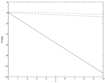
Figure 1. Upper bounds: $E_{var}$, solid line; $E_{W}$, dashed line; $E_{SC}$, dash-dotted line; $k_{0}=0.5$.

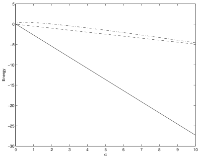
Figure 2. Upper bounds: $E_{var}$, solid line; $E_{W}$, dashed line; $E_{SC}$, dash-dotted line; $k_{0}=1$.

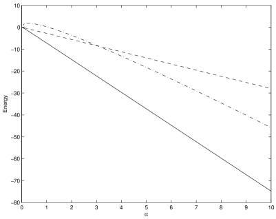
Figure 3. Upper bounds: $E_{var}$, solid line; $E_{W}$, dashed line; $E_{SC}$, dash-dotted line; $k_{0}=2$.

Figure 4. Upper bounds: $E_{var}$, solid line; $E_{W}$, dashed line; $E_{SC}$, dash-dotted line; $k_{0}=3$.

References

• [1] Landauย L.D., Phys. Z. Sowietunion, 1933, 3, 664. [English translation: Collected Papers. New York: Gordon and Breach, 1965.
• [2] Pekarย S.I., Sov. Phys. JETP, 1946, 16, 341. seeย also Pekarย S.I., Research in Electron Theory of Crystals. Moscow, Gostekhizdat, 1951. [English translation: Research in Electron Theory of Crystals. US AEC Report AEC-tr-5575].
• [3] Landauย L.D., Pekarย S.I., Sov. Phys. JETP, 1948, 18, 419.
• [4] H.ย Frรถhlich, H.ย Pelzer and S.ย Zienau, Philos. Mag. 41, 221 (1950).
• [5] Frรถhlichย H., Proc. Roy. Soc. A, 1937, 160, 230.
• [6] Frรถhlichย H., Advan. Phys., 1954, 3, 325.
• [7] Feynmanย R.P., Phys. Rev., 1955, 97, 660. seeย also R.ย P. Feynmanย R.P., Statistical Mechanics. Benjamin, Reading, MA, 1972.
• [8] Bogolubovย N.N., Ukrainian Math. J., 1950 II, No.ย 2, 3.
• [9] Bogolubovย N.N., Bogolubovย N.N. Jr., Aspects of the Polaron Theory. JINR Communications P-17-81-65, Dubna, 1981. seeย also Bogolubovย N.N., Bogolubovย N.N. Jr., Aspects of Polaron Theory. Equilibrium and Nonequilibrium Problems. World Scientific Publishing Company, New Jersey, london, Singapore, Beijing, Shanghai, Hong Kong, Taipei, Chennai, 2008.
• [10] Leeย T.D., Lowย F., Pinesย D., Phys. Rev., 1953, 90, 297.
• [11] Soldatovย A.V., Int. J. Mod. Phys. B, 1995, 9, n.22, 2899.
• [12] Peetersย F.M., Devreeseย J.T., J. Phys. A: Math. Gen., 1984, 17, 625.
• [13] Kireevย A.N., Int. J. Mod. Phys. B, 1997, 11, n.10, 1235.
• [14] Sumiย A, Toyozawaย Y., J. Phys. Soc. Jpn., 1973, 35, 137.
• [15] Peetersย F.M., Devreeseย J.T., Phys. Rev. B, 1985, 32, 3515.
• [16] Soldatovย A.V., Cond. Matter Phys., 2010, 13:4, 43701, 9 C.
• [17] Thomchickย J., Phys. Rev. B, 1978, 17, 1540.
Refer to caption