Adjusting chaotic indicators to curved spacetimes

Abstract

In this work, chaotic indicators, which have been established in the framework of classical mechanics, are reformulated in the framework of general relativity in such a way that they are invariant under coordinate transformation. For achieving this, the prescription for reformulating mLCE given by [Y. Sota, S. Suzuki, and K.-I. Maeda, Classical Quantum Gravity 13, 1241 (1996)] is adopted. Thus, the geodesic deviation vector approach is applied, and the proper time is utilized as measure of time. Following the aforementioned prescription, the chaotic indicators FLI, MEGNO, GALI, and APLE are reformulated. In fact, FLI has been reformulated by adapting other prescriptions in the past, but not by adapting the Sota et al. one. By using one of these previous reformulations of FLI, an approximative expression giving MEGNO as function of FLI has been applied on non-integrable curved spacetimes in a recent work. In the present work the reformulation of MEGNO is provided by adjusting the definition of the indicator to the Sota et al. prescription. GALI, and APLE are reformulated in the framework of general relativity for the first time. All the reformulated indicators by the Sota et al. prescription are tested and compared for their efficiency to discern order from chaos.

I Introduction

The concept of a chaotic dynamical system is usually correlated with the property of a system exhibiting sensitive dependence on initial conditions (see, e.g., the Devaney definition of chaos Devaney89 ). Even though this correlation might be somehow misleading (see, e.g., Banks94 ), the sensitivity to initial conditions provides an efficient way to detect chaos. Therefore, various such detecting methods have been developed and established in the framework of classical celestial mechanics over the last decades (see, e.g., Contop02 ; Skokos10 ; Maffione ).

From this variety of methods we are going to investigate a group of indicators which use the evolution of deviation vectors along a given orbit. In the classical framework the deviation vector evolves in a space tangential to the phase space, the measure of this vector is taken to be Euclidean, and the time is an independent parameter. From the category of these indicators, the most renowned is the maximal Lyapunov Characteristic Exponent (mLCE) (see, Skokos10 for a survey). Other similar indicators are: the Fast Lyapunov Indicator (FLI) Froesche97 ; Froesche05 , the Mean Exponential Growth of Nearby Orbits (MEGNO) Cincotta00 ; Cincotta03 , the Generalized Alignment Index (GALI) Skokos01 ; Skokos07 , the Average Power Law Exponent (APLE) LGVE08 ; LGVE09 . In classical mechanics the above mentioned indicators have been compared and studied for their efficiency several times (see, e.g., LGVE08 ; Maffione ).

However, the definition and the efficiency of these indicators pose issues in the framework of General Relativity (GR) (see, e.g., Motter ; Wu06 and references therein). Namely, one has to redefine the chaotic indicators in such a way that they will be invariant under coordinate transformations, and then to test these redefined indicators for their ability to detect chaos. In order to do the former, one has to find a way to define an invariant measure of the deviation vector in GR, and to choose an invariant time parameter. For the geodesic motion in curved spacetimes, which is the case we focus on, some suggestions to solve the above issues have already been provided. For instance, the indicators can be evaluated by applying the $3+1$ spacetime splitting approach Karas92 or by choosing the proper time as the time parameter Sota96 and using the invariant measure of the deviation vector either derived by the geodesic deviation equations Sota96 or by the two nearby orbits approximation Wu06 . In this study, the guideline of Sota et al. Sota96 was preferred for adjusting the chaotic indicators to the GR framework. However, if we depart from the geodesic motion, for example by taking into account the spin of the test particle, then approaches stemming from the $3+1$ splitting Karas92 are maybe preferable for addressing the aforementioned issues (see, e.g., Hartl03 ; Han08 ).

On the other hand, the above indicators are not the only methods which have been employed for detecting chaos in relativistic systems. Frequency analysis techniques, which were applied initially in the framework of classical mechanics (see, e.g., Laskar93 ), have been lately applied in the GR framework as well (see, e.g., SemSuk ; LG12 ); the same holds for the recurrence analysis techniques (see, Marwan07 for a review) which were also applied recently in curved spacetimes (see, e.g., Kopac ; SemSuk ). Both frequency analysis and recurrence analysis techniques are applied on time series, which makes them appropriate for the observational data post-analysis. Moreover, the recurrence analysis is able to discern deterministic chaos from stochastic noise, which might be very useful when the signal is embedded in noise.

Yet another kind of approach are the basin boundaries basin , which take advantage of the fractal geometry of a non-integrable system to detect the existence of chaos. The methods which use the curvature of a spacetime to search for chaos Sota96 ; Szyd are also Geometrical.

The background spacetime of a rapidly spinning neutron star suggested in MSM provides the non-integrable dynamical system to test the adjusted chaotic indicators. We are going to refer to this spacetime as Manko, Sanabria-Gómez, Manko or briefly MSM from now on. MSM background belongs to a broader family of spacetimes describing the surrounding spacetime of neutron stars; this family of spacetimes was introduced in Manko95 and revisited in Pappas13 , and their astrophysical importance was investigated in Pappas13 ; Berti04 . Now, from the dynamical point of view, since the existence of chaos in MSM background has already been revealed in Dubeibe07 ; Han08b ; Seyrich12 , the MSM spacetime provides the appropriate background for testing chaotic indicators on geodesic orbits.

The integration scheme applied to evolve these geodesic orbits along with the geodesic deviation equations is a symmetric, reversible integrator called integrator for geodesic equations of motion (IGEM) Seyrich12 . IGEM has been designed to evolve strongly chaotic orbits efficiently and to preserve the constants of motion. IGEM has been tested and compared with other integrators in the MSM spacetime Seyrich12 . From the above comparison IGEM appears to be the most appropriate for the present study.

The paper is organized as follows. Sec. II provides a brief description of the curved spacetime in which the chaotic indicators are tested. A brief survey on the geodesic and geodesic deviation equation of motion follows in Sec. III. The chaotic indicators and their invariant reformulation in curved spacetimes are presented in Sec. IV. Numerical examples of these indicators are given in Sec. V. Sec. VI surveys the main results, and in Appendix A the accuracy of the integrating scheme is discussed.

II The Manko, Sanabria-Gómez, Manko spacetime

It has been already mentioned that MSM belongs to a family of spacetimes that were designed to model neutron stars (see, e.g., Pappas13 ; Berti04 ). The MSM spacetime is asymptotically flat, axisymmetric and stationary; it describes the “exterior field of a charged, magnetized, spinning deformed mass” MSM . The MSM is a five-parameter vacuum solution, it depends on the mass $m$, the spin per unit mass $a$, the total charge $q$, the magnetic dipole moment ${\cal M}$, and the mass-quadrupole moment ${\cal Q}$. However, the two latter quantities are functions of the first three real parameters and of two other real parameters, i.e., $\mu$ and $b$,

$${\cal M} = \mu+q(a-b)~{}~{},$$

$${\cal Q} = -m(d-\delta-a~{}b+a^{2})~{}~{},$$ (1)

where

$$\delta := \frac{\mu^{2}-m^{2}b^{2}}{m^{2}-(a-b)^{2}-q^{2}}~{}~{},$$

$$d := \frac{1}{4}[m^{2}-(a-b)^{2}-q^{2}]~{}~{}.$$ (2)

The Weyl-Papapetrou line element of the MSM spacetime in prolate spheroidal coordinates $t,~{}x,~{}\phi,~{}y$ is

$$ds^{2}=g_{tt}~{}dt^{2}+g_{t\phi}dt~{}d\phi+g_{\phi\phi}+g_{xx}d\rho^{2}+g_{yy}dz^{2}~{}~{},\\$$ (3)

where

$$g_{tt} = -f~{}~{},$$

$$g_{t\phi} = f\omega~{}~{},$$

$$g_{\phi\phi} = \frac{k^{2}(x^{2}-1)(1-y^{2})}{f}-f\omega^{2}~{}~{},$$ (4)

$$g_{xx} = \frac{k^{2}e^{2\gamma}}{f}\frac{x^{2}-y^{2}}{x^{2}-1}~{}~{}.$$

$$g_{yy} = \frac{k^{2}e^{2\gamma}}{f}\frac{x^{2}-y^{2}}{1-y^{2}}~{}~{}.$$

The functions $f$, $\omega$, and $\gamma$ are

$$f = C/D~{}~{},$$

$$e^{2\gamma} = C/16k^{8}(x^{2}-y^{2})^{4}~{}~{},$$ (5)

$$\omega = (y^{2}-1)F/C~{}~{},$$

and

$$k:=\sqrt{d+\delta}~{}~{}.$$ (6)

The functions $C$, $D$, and $F$ are

$$C = R^{2}+\lambda_{1}\lambda_{2}S^{2}~{}~{},$$

$$D = E+RP+\lambda_{2}ST~{}~{},$$ (7)

$$F = RT-\lambda_{1}SP~{}~{},$$

where

$$\lambda_{1}=k^{2}(x^{2}-1),~{}~{}\lambda_{2}=y^{2}-1~{}~{}.$$ (8)

The functions $P$, $R$, $S$ and $T$ are

$$P := 2\{kmx[(2kx+m)^{2}-2y^{2}(2\delta+ab-b^{2})$$

$$- a^{2}+b^{2}-q^{2}]-2k^{2}q^{2}x^{2}-2y^{2}(4\delta d-m^{2}b^{2})\}~{}~{},$$

$$R := 4[k^{2}(x^{2}-1)+\delta(1-y^{2})]^{2}$$ (9)

$$+ (a-b)[(a-b)(d-\delta)-m^{2}b+q~{}\mu](1-y^{2})^{2}~{}~{},$$

$$S := -4{(a-b)[k^{2}(x^{2}-y^{2})+2\delta y^{2}]+y^{2}(m^{2}b-q~{}\mu)}~{}~{},$$

$$T := 4(2kmbx+2m^{2}b-q~{}\mu)[k^{2}(x^{2}-1)+\delta(1-y^{2})]$$

$$+ (1-y^{2})\{(a-b)(m^{2}b^{2}-4\delta d)$$

$$- (4kmx+2m^{2}-q^{2})[(a-b)(d-\delta)-m^{2}b+q~{}\mu]\}.$$

It is useful to mention that in the numerical calculations it is better to use the following combinations and expressions, in order to avoid numerical errors when the orbits approach the static limit $g_{tt}=C=0$,

$$\left[\frac{e^{2\gamma}}{f}\right] = \frac{D}{16k^{8}(x^{2}-y^{2})^{4}}~{}~{},$$

$$\left[f\omega\right] = \lambda_{2}\frac{F}{D}~{}~{},$$

and

$$g_{\phi\phi} = -\frac{\lambda_{2}}{D}\left[\lambda_{1}\left(C+2(RP+\lambda_{2}ST)\right)+\lambda_{1}P^{2}+\lambda_{2}T^{2}\right]$$

$$= -\left[2\lambda_{1}\lambda_{2}+\frac{\lambda_{2}}{D}(\lambda_{1}(P^{2}-E)+\lambda_{2}T^{2})\right]~{}~{}.$$

The numerical calculations were done in prolate spheroidal coordinates $x,~{}y$, but the results are presented in cylindrical coordinates $\rho,~{}z$ to facilitate the comparison with previous works Dubeibe07 ; Han08b ; Seyrich12 . The two coordinate systems relate through the transformation

$$\rho=k\sqrt{(x^{2}-1)(1-y^{2})},~{}~{}z=kxy~{}~{}.$$ (10)

III Geodesic and geodesic deviation

The fact that geodesic motion in MSM background exhibits chaotic behavior was shown in Dubeibe07 ; Han08b ; Seyrich12 mainly by studying Poincaré sections, but also by applying the FLI indicator Han08 as defined in Wu06 , and by the means of frequency analysis Seyrich12 .

For finding Poincaré sections, we have to evolve the geodesic equations

$$\ddot{x}^{\alpha}+\Gamma^{\alpha}_{\beta\gamma}\dot{x}^{\beta}\dot{x}^{\gamma}=0~{}~{},$$ (11)

where the dot corresponds to a derivative with respect to the proper time $\tau$, and $\Gamma^{\alpha}_{\beta\gamma}$ are the Christoffel symbols. The greek indices correspond to the whole spacetime.

The geodesic equations (11) are the Euler-Lagrange equations of the Lagrangian function

$$L=\frac{1}{2}g_{\alpha\beta}\dot{x}^{\alpha}\dot{x}^{\beta}~{}~{},$$ (12)

which is a constant of motion $L=-1$, and expresses the conservation of the four velocity of the test particle. The stationarity of the MSM spacetime provides the second constant

$$p_{t}=\frac{L}{\dot{t}}=-E~{}~{},$$ (13)

which is the energy of the test particle, while the axisymmetry provides the third constant

$$p_{\phi}=\frac{L}{\dot{\phi}}=L_{z}~{}~{},$$ (14)

which is the azimuthal component of the test particle’s angular momentum. By the last two constants the system is reduced to two degrees of freedom, and therefore, the Poincaré section can be used for detecting chaos in MSM spacetime backgrounds.

However, for including indicators in the study depending on deviation vectors like FLI, we need the geodesic deviation equations

$$\ddot{\xi}^{\alpha}+2\Gamma^{\alpha}_{\beta\gamma}\dot{x}^{\beta}\dot{\xi}^{\gamma}+\frac{\partial\Gamma^{\alpha}_{\beta\gamma}}{\partial x^{\delta}}\dot{x}^{\beta}\dot{x}^{\gamma}\xi^{\delta}=0~{}~{},$$ (15)

which show how two initially nearby geodesic orbits “$x^{\alpha}$” and “$x^{\alpha}+\xi^{\alpha}$” diverge from each other. $\xi^{\alpha}$ is the deviation vector, whose behavior plays a major role in distinguishing order from chaos as discussed in the next section.

IV Chaotic indicators

The measure of the deviation vector for a regular orbit grows linearly, while for a chaotic the growth is exponential or at least it follows a power law (see, e.g., LGVE08 ). This fact is the characteristic which mLCE, FLI, MEGNO, and APLE are designed to track. In order to have an invariant measure of the deviation vector in the phase space, Sota et al. Sota96 defined the quantity

$$\Xi^{2}=g_{\alpha\beta}\xi^{\alpha}\xi^{\beta}+g_{\alpha\beta}\frac{D\xi^{\alpha}}{d\tau}\frac{D\xi^{\beta}}{d\tau}~{}~{},$$ (16)

where the covariant derivative

$$\frac{D\xi^{\alpha}}{d\tau}=\dot{\xi}^{\alpha}+\Gamma^{\alpha}_{\beta\gamma}\dot{x}^{\beta}\xi^{\gamma}$$ (17)

provides the divergence of the velocities.

In order to ensure that $\Xi^{2}$ stays positive throughout the simultaneous evolution of the Eqs. (11), (15), we have to ensure that $\xi^{\alpha}$ and $\displaystyle\frac{D\xi^{\alpha}}{d\tau}$ will remain spacelike. The prescription for this Sota96 ; Wu06 is to choose initial conditions for $\xi^{\alpha},~{}\displaystyle\frac{D\xi^{\alpha}}{d\tau}$ such that

$$\xi^{\alpha}\dot{x}_{\alpha}=\frac{D\xi^{\alpha}}{d\tau}\dot{x}_{\alpha}=0~{}~{}.$$ (18)

However, condition (18) is not the only way to ensure $\Xi^{2}>0$, and in Wu06 other options are discussed. Anyway, for the numerical calculations done in this study the initial prescription of Sota et al. Sota96 is followed.

To address the issue of invariant time measure, whenever the definition of an indicator asks for a time parameter, the proper time is utilized. This parameter should be normalized by a typical time scale, e.g., $\tau_{ts}\approx Gm/c^{3}$ Sota96 . Throughout the article, geometric units are used, i.e., G=c=1, and the value of the mass $m$ of the central object is chosen to be of order of one, thus for simplicity, and without loss of generality, this time scale is set to be $\tau_{ts}=1$.

IV.1 mLCE

The maximal Lyapunov Characteristic Exponent

$$\textrm{mLCE}=\lim_{\tau\rightarrow\infty}\frac{1}{\tau}\ln{\frac{\Xi(\tau)}{\Xi(0)}}$$ (19)

is the most renowned chaotic indicator (see, Skokos10 for a review). The limit at infinity makes mLCE unrealistic for numerical studies, and the finite form of mLCE

$$\textrm{FmLCE}=\frac{1}{\tau}\ln{\frac{\Xi(\tau)}{\Xi(0)}}$$ (20)

is used instead. In Eq. (20) $\tau$ is sufficiently large. However, in the literature FmLCE is usually referred to as mLCE, which is adopted also in this article. Several techniques to find the invariant form of mLCE have already been suggested for geodesic flow in curved space, and a survey of these techniques can be found in Wu06 .

One category of these techniques uses a “shadow” orbit instead of evolving the geodesic deviation Eqs. (15). This shadow orbit is a geodesic orbit with initial conditions very near to the orbit under study, and the distance in the configuration space between these two orbits is used instead of $\Xi$. The shadow technique provides probably an easier way to discover whether an orbit is chaotic or not than the geodesic deviation technique does, because one just has to evolve two nearby orbits by computing the geodesic Eqs. (11). However, since the evolution of two orbits in a curved spacetime is not as exact as evolving the geodesic deviation Eqs. (15) in a spacetime tangent to the phase space where the orbital motion takes place, this approximation has a cost. Namely, even if we get a value of the mLCE near to the real mLCE (see, e.g., the numerical examples in Wu06 ), we lose the invariance of the mLCE indicator by using the shadow approximation.

The category of techniques using geodesic deviation equations splits into two subcategories. One subcategory uses the definition of $\Xi$ given by Sota et al. Sota96 (Eq. (16)) and the other measures the distance $\Xi$ only in the configuration space i.e., $\Xi^{2}=g_{\alpha\beta}\xi^{\alpha}\xi^{\beta}$. Now, the fact that the latter subcategory confines itself to a subspace of the space tangent to the phase space raises the question whether this technique can indeed find the invariant value of mLCE or it just distinguishes order from chaos, which would mean that this subcategory shares the same drawback with the technique of shadow orbits. On the other hand, the subcategory using the measure of $\Xi$ as given in Eq. (16) does not suffer from such ambiguity, since $\Xi$ is defined in the phase space. The latter has been in fact used for the reformulation of mLCE in Sota96 .

The principle of chaos detection behind the mLCE indicator is the following. When an orbit is regular, which means that on average $\Xi(\tau)$ grows linearly, then from Eq. (20) it is easy to show that

$$\textrm{mLCE}\propto\frac{\ln{\tau}}{\tau}~{}~{}.$$

Thus, for a regular orbit,

$$\lim_{\tau\rightarrow\infty}\textrm{mLCE}\rightarrow 0~{}~{}.$$

When an orbit is chaotic, which means usually that $\Xi(\tau)$ grows exponentially, e.g., $\Xi(\tau)\propto e^{\lambda\tau}$ where $\lambda$ is constant, then from Eq. (20) one gets

$$\textrm{mLCE}\propto\lambda~{}~{}.$$

Thus, for a chaotic orbit,

$$\lim_{\tau\rightarrow\infty}\textrm{mLCE}\rightarrow\lambda~{}~{}.$$

IV.2 FLI

The principles behind the mLCE indicator hold also for the Fast Lyapunov Indicator Froesche97 ; Froesche05 ,

$$\textrm{FLI}=\ln{\frac{\Xi(\tau)}{\Xi(0)}}~{}~{}.$$ (21)

The difference here is that in order to discern a chaotic orbit from a regular orbit, one has to define a time dependent limit. This limit depends on the maximum value of the FLI ($\textrm{FLI}_{max}$) that a regular orbit reaches at a given time. Then the $\textrm{FLI}_{max}$ value is compared with the FLI value reached by the other orbits at this given time. If the FLI value of an orbit is above $\textrm{FLI}_{max}$, then the orbit is characterized as chaotic. In fact, usually this limit is set as $\textrm{FLI}_{max}$ plus a relatively arbitrary “safety” value. For instance, if the maximum FLI value is $\textrm{FLI}_{max}$ in the finite proper time $\tau_{f}$, then the limit can be set to $\textrm{FLI}_{0}=\textrm{FLI}_{max}+\textrm{Constant}$, and any orbit whose $\textrm{FLI}>\textrm{FLI}_{0}$ is characterized as chaotic. For a detailed discussion on the $\textrm{FLI}_{0}$ issue refer to Sec. 3.2 of LGVE08 .

In the framework of general relativity a reformulation of FLI was proposed in Wu06 by employing the shadow orbit technique already discussed in Sec. IV.1. By the means of this approximative technique, FLI has already been applied in a few works (see, e.g., Han08b ; SemSuk ), but FLI has not yet been tested by applying the geodesic deviation technique according to the author’s knowledge.

IV.3 MEGNO

The basic definition of the Mean Exponential Growth of Nearby Orbits Cincotta00 ; Cincotta03 is

$$\textrm{MEGNO}(\tau_{f})=\frac{2}{\tau_{f}}\int_{0}^{\tau_{f}}\frac{\dot{\Xi}}{\Xi}\tau d\tau~{}~{},$$ (22)

where $\tau_{f}$ is the finite proper time until which the equations of motion (11), (15) are computed. A quite good approximation for MEGNO correlates it with the FLI indicator Mestre11 , i.e.,

$$\textrm{MEGNO}(\tau_{f})=2\left[\textrm{FLI}(\tau_{f})-<\textrm{FLI}(\tau_{f})>\right]~{}~{},$$ (23)

where $<\textrm{FLI}(\tau_{f})>$ is the mean value of FLI until the time $\tau_{f}$. However, MEGNO defined in the form (22) suffers from big value oscillations; for this reason, the average value of MEGNO,

$$<\textrm{MEGNO}(\tau_{f})>=\frac{1}{\tau_{f}}\int_{0}^{\tau_{f}}MEGNO(\tau)d\tau~{}~{},$$ (24)

is more useful. In fact, from now on we are going to refer to average MEGNO simply as MEGNO. The advantage of MEGNO over FLI is that it has a time independent limit by which an orbit is characterized as a chaotic or a regular one. For a regular orbit, MEGNO tends asymptotically to two, while if the orbit is chaotic it tends asymptotically to infinity.

Recently, in the last article of the SemSuk series, the MEGNO was tested in curved spacetimes describing a Schwarzschild black hole surrounded by a thin disc or a ring. The authors of this article used the approximation given by Eq. (23), and applied the shadow orbit technique to approximate the deviation vector. In the present study, another approach is followed. By using the approximation

$$\dot{\Xi}(\tau)=\frac{\Xi(\tau)-\Xi(\tau-d\tau)}{d\tau}~{}~{},$$

and by rewriting the formula (22) in discrete form, we arrive at

$$\textrm{MEGNO}(\tau_{f})=\frac{2}{\tau_{f}}\sum_{i=0}^{N}\left(1-\frac{\Xi(\tau_{i}-d\tau_{i})}{\Xi(\tau_{i})}\right)\tau_{i}~{}~{},$$ (25)

where $\displaystyle\tau_{f}=\sum_{i=0}^{N}\tau_{i}$. Respectively, the discrete form of Eq. (24) is

$$<\textrm{MEGNO}(\tau_{f})>=\frac{1}{\tau_{f}}\sum_{i=0}^{N}MEGNO(\tau_{i})d\tau_{i}~{}~{},$$ (26)

where $d\tau_{i}=\tau_{i}-\tau_{i-1}$ is practically the integration step used in the numerical calculations.

IV.4 APLE

The Average Power Law Exponent LGVE08 ; LGVE09 ,

$$\textrm{APLE}=\lim_{\tau\rightarrow\infty}\frac{\ln{\frac{\Xi(\tau)}{\Xi(0)}}}{\ln{\tau}}~{}~{},$$ (27)

was defined in order to detect “metastable” behaviors of weakly chaotic orbits. During this “metastable” phase the measure of the deviation vector increases following nearly a power law $\Xi(\tau)\propto\tau^{p}$. This phase ends when the measure of the vector begins to grow exponentially. Like the MEGNO, APLE has a limit to which regular orbits converge; this limit is the value one. If the orbit is weakly chaotic, then APLE will oscillate around a value equal to $p$ during the metastable phase. After the metastable phase, or if the orbit is strongly chaotic, the value of APLE goes to infinity following the exponential growth of the deviation vector.

In order to avoid a nullification of the denominator in Eq. (27), we can use various numerical tricks, which do not compromise the efficiency of the indicator (see, LGVE08 for a detailed discussion). For the purpose of this work, $\ln{(1+\tau)}$ was utilized; thus,

$$\textrm{APLE}=\lim_{\tau\rightarrow\infty}\frac{\ln{\frac{\Xi(\tau)}{\Xi(0)}}}{\ln{(1+\tau)}}$$ (28)

is used in the numerical examples of Sec. V instead of the Eq. (27). For $\tau>>1$, definition (27) is numerically equivalent to formula (28).

IV.5 GALI

The Generalized Alignment Index Skokos07 is a generalization of the Smaller Alignment Index (SALI) Skokos01 (also called Alignment Index Voglis02 ). GALI differs from the indicators discussed above because it does not depend on the rate by which a deviation vector grows, but on whether two or more deviation vectors with different initial directions will get aligned or not. GALI is identical to SALI when only two deviation vectors are used.

In particular, GALI uses the following properties of the deviation vectors. In the case of a chaotic orbit, two or more deviation vectors with different and arbitrary initial orientations will become parallel or anti-parallel exponentially fast. The speed by which this will happen depends on the value of the mLCE. On the other hand, in the case of regular motion, an orbit moves on a torus, and two or more deviation vectors with different and arbitrary initial orientations will become tangent to that torus with time. However, if the torus is $N$-dimensional, where $N\geq 2$, the orientation of the deviation vectors will remain, in general, different. If the torus is one-dimensional then the deviation vectors will become parallel or anti-parallel, but the time will follow a power law. Initially these properties have been investigated for the spectral distance techniques (see, e.g., VCE ), but by the introduction of SALI Skokos01 a more simple and efficient technique to detect chaos has been provided.

In Skokos01 SALI was defined as

$$\textrm{SALI}=\min{\left\{\left|\mathbf{w}-\mathbf{w}^{\prime}\right|,\left|\mathbf{w}+\mathbf{w}^{\prime}\right|\right\}}~{}~{},$$ (29)

where $\mathbf{w}$ and $\mathbf{w}^{\prime}$ are the deviation vectors of classical mechanics normalized to unity by their Euclidean norm. Another way to define SALI is to take the cross product of these vectors, .i.e.,

$$\textrm{SALI}=\left|\mathbf{w}\times\mathbf{w}^{\prime}\right|=\sin{\theta}~{}~{},$$ (30)

where $\theta$ is the angle between the two vectors. The definition (30) reveals that SALI, in fact, measures the surface defined by the two vectors.

In the case of a system with two degrees of freedom or more, SALI goes to zero for a chaotic orbit, while for a regular orbit it remains non-zero. In the case of a two dimensional map, SALI always goes to zero, but for chaotic orbits this happens exponentially fast, while for regular orbits $\textrm{SALI}\propto t^{-q}$, where $q\approx 2$. This kind of power laws, in fact, provide the means for GALI to find the dimension of a torus in multidimensional systems Skokos07 . The advantage of GALI over the other indicators is exactly this ability, but in order to use it, we have to evolve more than two deviation vectors. Thus, the advantage of GALI comes with a certain computational cost.

In curved spacetimes the Euclidean norm is not invariant under coordinate transformations, thus we cannot normalize the generalized deviation vector (Eq. (16)) defined by $\xi^{\alpha}$ and $\displaystyle\frac{D\xi^{\alpha}}{d\tau}$ to unity. This certainly is a problem for the definition (29), because for parallel vectors $\left|\mathbf{w}-\mathbf{w}^{\prime}\right|$ will not go to zero and for anti-parallel vectors $\left|\mathbf{w}+\mathbf{w}^{\prime}\right|$ will not go to zero.

On the other hand, in the definition (30) we really don’t depend on the strict normalization of the deviation vector to unity, the only thing we need is to limit the growth of the components $\xi^{\alpha}$ and $\displaystyle\frac{D\xi^{\alpha}}{d\tau}$. In order to do that we can divide them by the measures of the corresponding vectors, i.e., $\displaystyle\frac{\xi^{\alpha}}{\sqrt{\xi_{\kappa}\xi^{\kappa}}}$ and $\displaystyle\frac{\frac{D\xi^{\alpha}}{d\tau}}{\sqrt{\frac{D\xi_{\kappa}}{d\tau}\frac{D\xi^{\kappa}}{d\tau}}}$. Then we can use the outer products of one pair $\xi^{\alpha}$, $\zeta^{\alpha}$ of the deviation vectors and their corresponding velocities $\displaystyle\frac{D\xi^{\alpha}}{d\tau}$ $\displaystyle\frac{D\zeta^{\alpha}}{d\tau}$ to provide a similar definition of SALI to Eq. (30), i.e.,

$$OI_{\alpha\beta} = \eta_{\alpha\beta\gamma\delta}\frac{\xi^{\gamma}}{\sqrt{\xi_{\kappa}\xi^{\kappa}}}\frac{\zeta^{\delta}}{\sqrt{\zeta_{\nu}\zeta^{\nu}}}~{}~{},$$ (31)

$$OII_{\alpha\beta} = \eta_{\alpha\beta\gamma\delta}\frac{\frac{D\xi^{\gamma}}{d\tau}}{\sqrt{\frac{D\xi_{\kappa}}{d\tau}\frac{D\xi^{\kappa}}{d\tau}}}\frac{\frac{D\zeta^{\delta}}{d\tau}}{\sqrt{\frac{D\zeta_{\nu}}{d\tau}\frac{D\zeta^{\nu}}{d\tau}}}~{}~{},$$ (32)

where $\eta_{\alpha\beta\gamma\delta}$ is the Levi-Civita density tensor

$$\eta_{\alpha\beta\gamma\delta}=\sqrt{-g}~{}\epsilon_{\alpha\beta\gamma\delta}~{}~{},$$ (33)

and $\epsilon_{\alpha\beta\gamma\delta}$ is the Levi-Civita symbol with $\epsilon_{0123}=-1$.

If the deviation vectors $\xi^{\alpha}$, $\zeta^{\alpha}$ and their velocities $\displaystyle\frac{D\xi^{\alpha}}{d\tau}$, $\displaystyle\frac{D\zeta^{\alpha}}{d\tau}$ are parallel, then both $OI_{\alpha\beta}$ and $OII_{\alpha\beta}$ are null. Thus, we can define the quantity

$$SALI=\sum_{\alpha=0}^{3}\sum_{\beta=0}^{3}\left(OI_{\alpha\beta}+OII_{\alpha\beta}\right)~{}~{},$$ (34)

which will go to zero for chaotic orbits and remain non-zero for regular orbits. In order to define GALI, we can use outer products for multiple deviation vectors and their corresponding velocities similar to (31), and sum these outer products as has been suggested for SALI in Eq. (34).

V Numerical examples

In order to check the ability of the adjusted indicators (discussed in Sec. IV) to discern chaos from order, it is better to start with cases where chaos has already been found. In these cases the indicators just have to verify the previous findings. Thus, the study starts with two cases of the MSM spacetime background, which were investigated in Han08b .

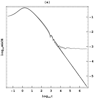
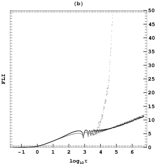
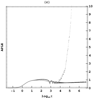
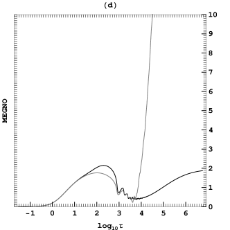
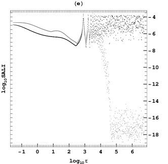
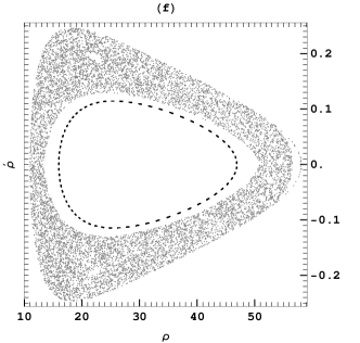
Figure 1: The behavior of chaotic indicators for two geodesic orbits, one regular (black) and one chaotic (gray), evolving in a MSM spacetime with $m=2.904$, $a=1.549$, $q=0$, $\mu=0$ and $b=6$. The constants of motion are $E=0.96$ and $L_{z}=2.75~{}m$. Panel (a) shows the evolution of mLCE as function of the proper time $\tau$ in logarithmic scale, panel (b) shows the FLI as function of $\log_{10}\tau$, panel (c) shows the APLE, panel (d) the MEGNO, panel (e) the $\log_{10}\textrm{SALI}$ as function of $\log_{10}\tau$, and panel (f) shows the Poincaré section on the equatorial plane $z=0$.

The first case comes from Fig. 3 of Han08 , where the mass is $m=2.904$, the spin is $a=1.549$, the charge is $q=0$, and the two real parameters are $\mu=0$ and $b=6$. In fact, for all the MSM spacetimes in this work the charge $q$ and the parameter $\mu$ were set to zero like in previous studies Dubeibe07 ; Han08b . The constants of motion in this example are $E=0.96$ and $L_{z}=2.75~{}m$. In Fig. 1, behaviors of different chaos detection techniques are shown for a regular orbit (black) and a chaotic orbit (gray). The initial radial distance for the former orbit is $\rho=16$, and for the latter $\rho=11$, while for both of them $\dot{\rho}=z=0$, and the $\dot{z}$ is derived from Eq. (12) with positive sign. The initial deviation vector used for Figs. 1(a)-(d) has $\xi^{x}=10^{-4}$, $\dot{\xi}^{x}=10^{-3}$, and $\dot{\xi}^{y}$ was calculated from the conditions (18), while the other components of the deviation vector and its derivative were set to zero. For the SALI in Fig. 1(e) a second deviation vector has been used, which initially has $\zeta^{\phi}=10^{-3}$ and $\dot{\zeta}^{x}=10^{-1}$; $\dot{\zeta}^{y}$ was evaluated from the conditions (18), while the other components of the deviation vector and its derivative were set to zero. Both deviation vectors satisfy the conditions (18). The preservation of these conditions and in general the numerical accuracy of the investigation is discussed in the Appendix A.

The Poincaré section ($z=0$, $\dot{z}>0$) of the orbits is shown in Fig. 1(f) (Fig. 3 of Han08 has more details). The chaotic orbit evolves in a chaotic sea (gray dots); thus we expect it to be strongly chaotic, while the regular orbit belongs to the resonance $9/65$ and it forms a chain of small islands of stability appearing like a “dashed” black curve.

In Fig. 1(a), the $\log_{10}\textrm{mLCE}$ is plotted as function of $\log_{10}{\tau}$. In such plots the curve of regular orbits tends to zero with a slop $\frac{\log_{10}\textrm{mLCE}}{\log_{10}{\tau}}\propto-1$ (see the discussion in Sec. IV.1), even if the curve of chaotic orbits can follow the slop $-1$ for a while, when the curve reaches the value of mLCE it becomes horizontal. The behavior described above is what we see in Fig. 1(a). Namely, the black points of the regular orbit follow the slope $-1$ as mLCE tends to zero, and the gray points showing the evolution of the chaotic orbit follow the $-1$ slope for a while, but after the time $\tau\approx 10^{-3}$ they change their inclination and become horizontal indicating the corresponding mLCE value ($\log_{10}\textrm{mLCE}\approx-3.15$).

The black points of the regular orbit in Fig. 1(b) show the anticipated linear growth of the corresponding deviation vector; i.e., we can see that $\textrm{FLI}\propto\log_{10}\tau$. The oscillations in FLI’s value come from the fact that the tori on which the regular orbits are evolving are not in general direct products of circles, but rather products of ellipses; thus, the deviation vector’s components stress and shrink periodically (for more details on these oscillations see e.g., the discussion in LGVE08 ). On the other hand, the gray points of the chaotic orbit, after a certain period that they behave similarly to the regular orbit, begin to diverge from the regular behavior with time because the exponential growth of the deviation vector dominates. Thus, until the time of this divergence we cannot distinguish a chaotic orbit from a regular one. The level a regular orbit reaches at a certain time indicates the threshold above which we can characterize an orbit as chaotic or regular (Sec. IV.2). However, this threshold is not only time-dependent, but also a little bit arbitrary because we have to include a safety margin for the oscillations (see Sec. IV.2 and discussion in LGVE08 ).

Examples of indicators with a time-independent threshold are the APLE and the MEGNO. These indicators for regular orbits tend asymptotically to $1$, and $2$, respectively (black points in Figs. 1(c)-(d)). In our examples, (Figs. 1(c)-(d)) the indicators tend to their asymptotic values from below (smaller values than the threshold); however, this is not always the case and the asymptotic behavior may be from above (see, e.g., LG12 ). Moreover, we have to take into account the oscillations of the deviation vector as we did for FLI. Thus, it is better to set higher values than the theoretical values to these thresholds, in order not to characterize regular orbits as chaotic. The actual thresholds’ values are usually set empirically, but they are not much higher than the theoretical ones. Now, for chaotic orbits the values of APLE and MEGNO tend to infinity, which is the case for the corresponding gray points shown in Fig. 1(c)-(d).

SALI differs from the other 4 indicators not only by the fact that it doesn’t take advantage of the deviation vector’s growth (in fact SALI kills this growth by normalizing the components of the deviation vectors), but also by the fact that it needs two deviation vectors with different initial orientations in order to distinguish regular from chaotic orbits. For regular orbits SALI oscillates around a non-zero value (black dots in Fig. 1(e)), while for chaotic orbits SALI initially also oscillates around a non-zero value, but afterwards it plunges to zero (gray dots in Fig. 1(e)). The oscillations ($10^{-14}\lesssim SALI\lesssim 10^{-19}$) for the chaotic orbit at large values of proper time in Fig. 1(e) are artificial, and they result from numerical round offs in the summation of Eq. (34). Thus, we have to set a quite arbitrary semi-empirical threshold, as was previously done for the other indicators, in order to characterize an orbit as chaotic. For example in the case of Fig. 1(e) this could be set to $10^{-10}$.

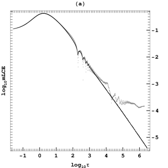
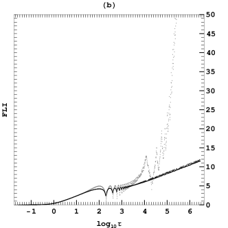
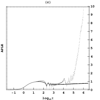
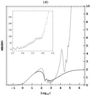
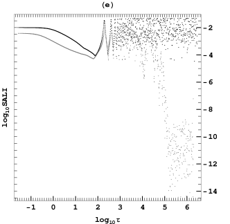
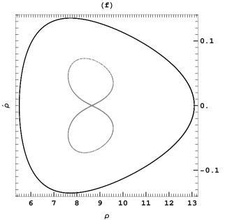
Figure 2: The behavior of chaotic indicators for two geodesic orbits, one regular (black) and one chaotic (gray), evolving in a MSM spacetime with $m=1.$, $a=0.6$, $q=0$, $\mu=0$ and $b=3$. The constants of motion are $E=0.95$ and $L_{z}=3$. Panel (a) shows the evolution of mLCE as function of the proper time $\tau$ in logarithmic scale, panel (b) shows the FLI as function of $\log_{10}\tau$, panel (c) shows the APLE, panel (d) the MEGNO (the embedded panel shows the non-averaged MEGNO), panel (e) the $\log_{10}\textrm{SALI}$ as function of $\log_{10}\tau$, and panel (f) shows the Poincaré section on the equatorial plane $z=0$.

The second example comes from Fig. 4 of Han08b , where the parameters of the MSM spacetime are $m=1$, $a=0.6$, and $b=3$, while the test particle has $E=0.95$ and $L_{z}=3$. The indicators seen in Figs. 2(a)-(e) were computed with the same initial deviation vectors’ setup as in Fig. 1. The black points correspond to the regular orbit with initial radial distance $\rho=5.5$, while the chaotic orbit has $\rho=8.65$. Both orbits started with $z=\dot{\rho}=0$, while $\dot{z}$ has been derived from Eq. (12). The Poincaré section for these orbits is shown in Fig. 2(f), the black curve shows a KAM, while the gray curve shows an orbit evolving in a chaotic layer inside the main island of stability.

The mLCEs of chaotic orbits moving in chaotic layers like the one in Fig. 2(f) are usually smaller than the mLCEs of chaotic orbits moving in a chaotic sea (e.g., Fig. 1(f)), when the chaotic orbits belong to the same Poincaré section. It is rather coincidental that this holds also when we compare the mLCE (gray dots) in Fig. 2(a)) with that in Fig. 1(a), because the orbits in Fig. 1 evolve in a different MSM spacetime than the orbits in Fig. 2. In such layers chaotic orbits tend to stick for considerable intervals of time near a regular orbit, and to imitate its behavior, this phenomenon is called stickiness (see Contop02 for a review on the stickiness phenomenon). For instance, if a chaotic orbit moving in a chaotic layer seems to give the final value of mLCE (Fig. 2(a) until $\log_{10}\tau\approx 5.5$), then if the orbit gets sticky, the mLCE will start dropping following a slope similar to a regular orbit (see the small drop in the mLCE value at $5.5\lesssim\log_{10}\tau\lesssim 6$ in Fig. 2(a)). After the orbit leaves the sticky region mLCE grows again (Fig. 2(a)). Thus, the adjusted mLCE to curved spacetimes is able to detect fine structures in the phase space.

Recall that FLI stands for fast Lyapunov indicator; thus, FLI has been designed to indicate the chaotic nature of an orbit quickly. For example, in Fig. 2(b) FLI has indicated that the orbit is chaotic at $\log_{10}\tau\approx 5$, while mLCE gives this indication at $\log_{10}\tau\approx 5.5$ (Fig. 2(a)), because we have to wait awhile until we are reassured that the mLCE has stopped dropping following the $-1$ inclination. However, this delay is not always the case; for example, Figs. 1(a),(b) show a case for which the detection needs approximately the same order of time, because the oscillations of FLI compel us to give a larger boundary to the limit for which we would characterize an orbit as chaotic (see previous discussions).

APLE, and MEGNO are as quick as FLI in detecting the chaoticity of an orbit (e.g., Figs. 2(b)-(d) and Figs. 1(b)-(d)), and they show the same sensitivity in detecting the stickiness interval. In particular, in Fig. 2(c) only a small break in the rate at which APLE tends to infinity can be seem for $5.5\lesssim\log_{10}\tau\lesssim 6$. FLI can detect this stickiness interval in the same way, but the change in this inclination is nearly visible like for APLE in Fig. 2. However, the MEGNO without the averaging (Eq. (25)) produces an observable plateau (embedded panel in Fig. 2(d)), during the time the orbit is sticky. The averaging is the reason why this plateau disappears in the averaged MEGNO and only a break in the rate gives away the stickiness. Thus, like in the case of mLCE, the reformulated chaotic indicators discussed in this paragraph, and in particular the reformulated MEGNO, are able to detect fine structures.

On the other hand, even if SALI is as fast as FLI, APLE and MEGNO in detecting chaos, there is no apparent evidence of stickiness in Fig. 2(e). It appears that once the deviation vectors become parallel, they do not diverge again.

The two examples (Figs. 1, 2) show that the readjusted indicators have the behavior which we would expect from their classical definition. In general, all the indicators have the same time response in detecting chaos, and this time depends on the maximum Lyapunov characteristic exponent. However, each of them has a special ability, which can make it ideal when a specific investigation of a dynamical system is required; e.g., APLE was designed to detect power law governed metastable behaviors. However, when the only aim is chaos detection, the indicator one chooses is a matter of convenience and taste.

             

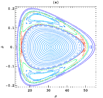
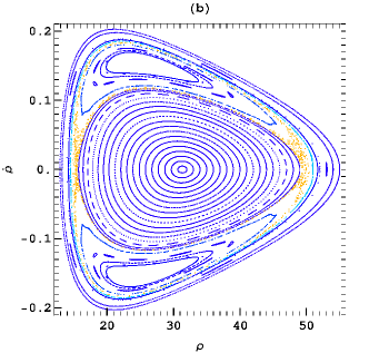
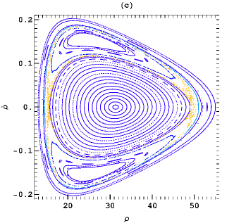
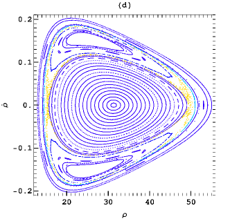
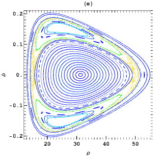
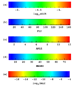
Figure 3: The values of the chaotic indicators on the Poincaré section lying on the equatorial plane $z=0$. The orbits evolve in a MSM spacetime with $m=2.904$, $a=1.549$, $q=0$, $\mu=0$ and $b=6$. The constants of motion are $E=0.96$ and $L_{z}=3.~{}m$. Panels (a)-(e) show the values of mLCE, FLI, APLE, MEGNO, and $\log_{10}\textrm{SALI}$ respectively in scales shown at the bottom right corner of the figure.

In order to reinforce the above point, the values of the five indicators under discussion are plotted on a Poincaré section in Fig. 3. This Poincaré section lies on the equator $z=0$ and has $\dot{z}>0$. The scales of the indicators’ values are given in the bottom right corner of Fig. 3. The orbits evolve in a MSM spacetime with $m=2.904$, $a=1.549$, $b=6$, and the constants of the motion are $E=0.96$, $L_{z}=3.~{}m$. For all orbits the initial deviation vectors are the same as those in Figs. 1, 2, and all five indicators have been evaluated for $1000$ sections. All five show clearly which regions are dominated by chaotic orbits and which by regular motion.

VI Conclusions

The chaotic indicators mLCE, FLI, GALI, MEGNO, and APLE had been defined in the framework of classical mechanics. In order to make these indicators appropriate for studying geodesic motion in curved spacetimes, they have to be reformulated in a way that will make them invariant under coordinate transformations. The authors of Sota96 provided a guideline to do this when they reformulated mLCE. By following this guideline the other four chaotic indicators were reformulated accordingly in Sec. IV. All the five reformulated indicators were tested in Sec. V for their efficiency in discerning regular from chaotic motion in the MSM spacetime background. It was shown that these five indicators have inherited the anticipated behavior from their classical counterparts, they are reliable, and, in general, equally fast in detecting chaotic motion.

Appendix A Numerical accuracy

For integrating the geodesics Eq. (11) and their deviations Eq. (15) the IGEM integration scheme Seyrich12 was implemented. This scheme was designed to cope with strongly chaotic geodesic motion efficiently and accurately. In this section we discuss IGEM’s performance.

One point not included in our previous analysis Seyrich12 is the renormalization of evaluated quantities during the evolution. The renormalization is applied in order to avoid the occurrence of very large numbers, which aside from causing other problems would slow down the IGEM integration scheme. These very large numbers appear due to the fact that the measure of the deviation vector grows exponentially; thus, in order to get rid of the growth of the corresponding values we renormalize them. In fact the renormalization of the deviation vector is a common ground in dynamical studies. Hence, anytime $\Xi$ becomes larger than $10$, the components of the deviation vector and the components of its velocity are multiplied by $10^{-2}$. However, there are times at which the measure of $\Xi$ can become very small; in such cases IGEM would choose its integrating step by taking into account mainly the needs of the geodesic orbit. In order to avoid this, anytime $\Xi$ drops below $10^{-3}$, the aforementioned components are divided by $10^{-2}$. Thus, by renormalization, the IGEM scheme is kept accurate and fast.

There are three independent and in involution constants of motion, namely, the energy $E$, the $z$ component of the angular momentum $L_{z}$, and the Lagrangian function $L$ itself. The Lagrangian function contains all the variables involved in the geodesic motion; thus, it is a very efficient quantity to check the accuracy of the numerical scheme applied. There are two relative errors that are of interest: first, the relative error between two time steps, i.e., $\log_{10}\left|1-\frac{L(\tau)}{L(\tau-d\tau)}\right|$, and the overall relative error, i.e., $\log_{10}\left|1-\frac{L(\tau)}{L}\right|$, where $L(\tau)$ is the value of the Lagrangian function evaluated at time $\tau$. Fig. 4(a) shows that the relative error between two time steps is of the order of the machine precision; however, the overall relative error seems to grow following a power law with exponent $\approx 5/9$ (Fig. 4(b)). This behavior appears to be independent of the character of the orbit; i.e., it does not depend on whether the orbit is chaotic (gray points) or regular (black points).

The deviation vectors $\xi^{\alpha}$, $\zeta^{\alpha}$ were set to satisfy the constraints (18) during the evolution of the orbits of Fig. 1. Panels (c)-(d) show how much these constraints were preserved. The slopes in these panels again indicate power laws, but each of them has a different exponent.

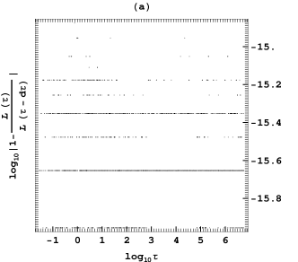
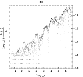
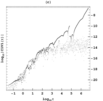
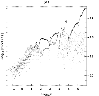
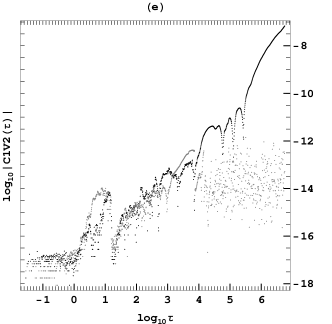
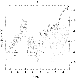
Figure 4: Accuracy checks of IGEM for the two orbits shown in Fig. 1. The black points correspond to the regular orbit, while the gray to the chaotic. Panel (a) shows the relative error between two time steps $\log_{10}\left|1-\frac{L(\tau)}{L(\tau-d\tau)}\right|$, where the $L(\tau)$ is the value of the Lagrangian function evaluated at time $\tau$. Panel (b) shows the overall relative error $\log_{10}\left|1-\frac{L(\tau)}{L}\right|$, where $L$ is the theoretical value of the Lagrangian function. Panels (c) and (d) show the conservation of the constraints $\xi^{\alpha}\dot{x}_{\alpha}=0$ (C1V1) and $\frac{D\xi^{\alpha}}{d\tau}\dot{x}_{\alpha}=0$ (C2V1) (Eq. (18)) respectively for the first vector, while panels (e) and (f) show the conservation of the constraints $\zeta^{\alpha}\dot{x}_{\alpha}=0$ (C1V2) and $\frac{D\zeta^{\alpha}}{d\tau}\dot{x}_{\alpha}=0$ (C2V2) respectively for the second vector.

References

- (1) R.L. Devaney, “An introduction to chaotic dynamical systems”, (Addison-Wesley Publishing Company, New York, 1989)
- (2) J. Banks, J. Brooks, G. Cairns, G. Davis, and P. Stacey, Am. Math. Mon. 99 332 (1992)
- (3) G. Contopoulos, “Order and chaos in dynamical astronomy” (Springer, Berlin, 2002)
- (4) C. Skokos, Lect. Notes Phys. 790, 63 (2010)
- (5) N. P. Maffione, L. A. Darriba, P. M. Cincotta, and C. M. Giordano, Celest. Mech. Dyn. Astron. 111, 285 (2011); Mon. Not. R. Astron. Soc. 429, 2700 (2013)
- (6) C. Froeschlé, R. Gonczi, and E. Lega, Planetary Space Sci. 45, 881 (1997)
- (7) C. Froeschlé, M. Guzzo, and E. Lega, Celest. Mech. Dyn. Astron. 92, 243 (2005)
- (8) P.M. Cincotta, and C. Simó, Astron. Astrophys. Sup. 147, 205 (2000)
- (9) P.M. Cincotta, C.M. Giordano, and C. Simó, Phys. D 182, 151 (2003)
- (10) C. Skokos, J. Phys. A: Math. Gen. 34, 10029 (2001)
- (11) C. Skokos, T. C. Bountis, and C. Antonopoulos, Phys. D , 231, 30 (2007)
- (12) G. Lukes-Gerakopoulos, N. Voglis, and C. Efthymiopoulos, Phys. A 387, 1907 (2008)
- (13) G. Lukes-Gerakopoulos, N. Voglis, and C. Efthymiopoulos, Chaos in Astronomy, 363 (2009)
- (14) A. E. Motter, Phys. Rev. L. 91, 231101 (2003); K. Gelfert, and A. E. Motter, Commun. Math. Phys. 300, 411 (2010)
- (15) Y. Sota, S. Suzuki, and K.-I. Maeda, Classical Quantum Gravity 13, 1241 (1996)
- (16) X. Wu, T.-Y. Huang, and H. Zhang, Phys. Rev. D 74, 083001 (2006)
- (17) V. Karas, and D. Vokrouhlicky, Gen. Rel. Grav. 24, 729 (1992)
- (18) M. D. Hartl, Phys. Rev. D 67, 024005 (2003); 67, 104023 (2003)
- (19) W. Han, Gen. Rel. Grav. 40, 1831 (2008)
- (20) J. Laskar, Celest. Mech. Dyn. Astron. 56, 19 (1993)
- (21) O. Semerák, and P. Suková, Mon. Not. R. Astron. Soc. 404, 545 (2010); 425, 2455 (2012); P. Suková, and O. Semerák, Mon. Not. R. Astron. Soc. 436, 978 (2013)
- (22) G. Lukes-Gerakopoulos, Phys. Rev. D 86, 044013 (2012)
- (23) N. Marwan, M. Carmen Romano, M. Thiel, and J. Kurths, Phys. Reports 438, 237 (2007)
- (24) O. Kopáček, V. Karas, J. Kovář, and Z. Stuchlík, Astroph. J. 722, 1240 (2010); J. Kovář, O. Kopáček, V. Karas, and Y. Kojima, Classical Quantum Gravity 30, 025010 (2013)
- (25) C. P. Dettmann, N. E. Frankel, and N. J Cornish, Phys. Rev. D 50, 618 (1994); N. J. Cornish, and N. E. Frankel, Phys. Rev. D 56, 1903 (1997); N. J. Cornish, and J. Levin, Phys. Rev. D 68, 024004 (2003)
- (26) M. Szydłowski, Phys. Lett. A 176, 22 (1993); M. Szydłowski, and A. Krawiec, Phys. Rev. D 53, 6893 (1996)
- (27) V. S. Manko, J. D. Sanabria-Gómez and O. V. Manko, Phys. Rev. D 62, 044048 (2000)
- (28) V. S. Manko, J. Martín, and E. Ruiz, Phys. Rev. D 51, 4187 (1995)
- (29) G. Pappas, and T. A. Apostolatos, Mon. Not. R. Astron. Soc. 429, 3007 (2013)
- (30) E. Berti, and N. Stergioulas, Mon. Not. R. Astron. Soc. 350, 1416 (2004)
- (31) F. L. Dubeibe, L. A. Pachón and J. D. Sanabria-Gómez, Phys. Rev. D 75, 023008 (2007)
- (32) W.-B. Han, Phys. Rev. D 77, 123007 (2008)
- (33) J. Seyrich, and G. Lukes-Gerakopoulos, Phys. Rev. D 86, 124013 (2012)
- (34) M. F. Mestre, P. M. Cincotta, and C. M Giordano, Mon. Not. R. Astron. Soc. 414, L100 (2011)
- (35) N. Voglis, C. Kalapotharakos, and I. Stavropoulos, Mon. Not. R. Astron. Soc. 337, 619 (2002)
- (36) N. Voglis, G. Contopoulos, and C. Efthymiopoulos, Phys. Rev. E 57, 372 (1998); Celest. Mech. Dyn. Astron. 73, 211 (1999)