A McKean optimal transportation perspective on Feynman-Kac formulae with application to data assimilation

Abstract

Data assimilation is the task of combining mathematical models with observational data. From a mathematical perspective data assimilation leads to Bayesian inference problems which can be formulated in terms of Feynman-Kac formulae. In this paper we focus on the sequential nature of many data assimilation problems and their numerical implementation in form of Monte Carlo methods. We demonstrate how sequential data assimilation can be interpreted as time-dependent Markov processes, which is often referred to as the McKean approach to Feynman-Kac formulae. It is shown that the McKean approach has very natural links to coupling of random variables and optimal transportation. This link allows one to propose novel sequential Monte Carlo methods/particle filters. In combination with localization these novel algorithms have the potential of beating the curse of dimensionality, which has prevented particle filters from being applied to spatially extended systems.

26/09/2013

1 Introduction

This paper is concerned with Monte Carlo methods for approximating expectation values for sequences of probability density functions (PDFs) $\pi^{n}(z)$, $n\geq 0$, $z\in{\cal Z}$. We assume that these PDFs arise sequentially from a Markov process with given transition kernel $\pi(z|z^{\prime})$ and are modified by weight functions $G^{n}(z)\geq 0$ at each iteration index $n\geq 1$. More precisely, the PDFs satisfy the recursion

$$\pi^{n}(z)=\frac{1}{C}G^{n}(z)\int_{\cal Z}\pi(z|z^{\prime})\pi^{n-1}(z^{\prime}){\rm d}z^{\prime}$$ (1)

with the constant $C$ chosen such that $\int_{\cal Z}\pi^{n}(z){\rm d}z=1$.

A general mathematical framework for such problems is provided by the Feynman-Kac formalism as discussed in detail in del Moral (2004). In order to apply Monte Carlo methods to (1) it is useful to reformulate (1) in terms of modified Markov processes with transition kernel $\pi^{n}(z|z^{\prime})$, which satisfy the consistency condition

$$\pi^{n}(z)=\int_{\cal Z}\pi^{n}(z|z^{\prime})\pi^{n-1}(z^{\prime}){\rm d}z^{\prime}.$$ (2)

This reformulation has been called the McKean approach to Feynman-Kac models in del Moral (2004). Once a particular McKean model is available, a Monte Carlo implementation reduces to sequences of particles $\{z_{i}^{n}\}_{i=1}^{M}$ being generated sequentially by

$$z_{i}^{n}\sim\pi^{n}(\cdot|z_{i}^{n-1}),\qquad i=1,\ldots,M,$$ (3)

for $n=0,1,\ldots,N$. In other words, $z^{n}_{i}$ is the realization of a random variable with (conditional) PDF $\pi^{n}(z|z_{i}^{n-1})$. Such a Monte Carlo method constitutes a particular instance of the far more general class of sequential Monte Carlo methods (SMCMs) (Doucet et al., 2001).

While there are many applications that naturally give rise to Feynman-Kac formulae (del Moral, 2004), we will focus in this paper on Markov processes for which the underlying transition kernel $\pi(z|z^{\prime})$ is determined by a deterministic dynamical system and that we wish to estimate its current state $z^{n}$ from partial and noisy observations $y^{n}_{\rm obs}$. The weight function $G^{n}(z)$ of a Feynman-Kac recursion (1) is in this case given by the likelihood of observing $y_{\rm obs}^{n}$ given $z^{n}$ and we encounter a particular application of Bayesian inference (Jazwinski, 1970; Stuart, 2010). The precise mathematical setting and the Feynman-Kac formula for the associated data assimilation problem will be discussed in Section 2. Some of the standard Monte Carlo approaches to Feynman-Kac formulae will be summarized in Section 3.

It is important to note that the consistency condition (2) does not specify a McKean model uniquely. In other words, given a Feynman-Kac recursion (1) there are many options to define an associated McKean model $\pi^{n}(z|z^{\prime})$. It has been suggested independently by Reich (2011); Reich and Cotter (2013) and Moselhy and Marzouk (2012) in the context of Bayesian inference that optimal transportation (Villani, 2003) can be used to couple the prior and posterior distributions. This idea generalizes to all Feynman-Kac formulae and leads to optimal in the sense of optimal transportation McKean models. This optimal transportation approach to McKean models will be developed in detail in Section 4 of this paper.

Optimal transportation problems lead to a nonlinear elliptic PDE, called the Monge-Ampere equation (Villani, 2003), which is very hard to tackle numerically in space dimensions larger than one. On the other hand, optimal transportation is an infinite-dimensional generalization (McCann, 1995; Villani, 2009) of the classic linear transport problem (Strang, 1986). This interpretation is very attractive in terms of Monte Carlo methods and gives rise to a novel SMCM of type (3), which we call the ensemble transform particle filter (ETPF) (Reich, 2013a). The ETPF is based on a linear transformation of the forecast particles

$$z_{i}^{f}\sim\pi(\cdot|z_{i}^{n-1}),\qquad i=1,\ldots,M,$$ (4)

of type

$$z_{j}^{n}=\sum_{i=1}^{M}z_{i}^{f}s_{ij}$$ (5)

with the entries $s_{ij}\geq 0$ of the transform matrix $S\in\mathbb{R}^{M\times M}$ being determined by an appropriate linear transport problem. Even more remarkably, it turns out that SMCMs which resample in each iteration as well as the popular class of ensemble Kalman filters (EnKFs) (Evensen, 2006) also fit into the linear transform framework of (5). We will discuss particle/ensemble-based sequential data assimilation algorithms within the unifying framework of linear ensemble transform filters in Section 5. This section also includes an extension to spatially extended dynamical systems using the concept of localization (Evensen, 2006). Section 7 provides numerical results for the Lorenz-63 (Lorenz, 1963) and the Lorenz-96 (Lorenz, 1996) models. The results for the 40 dimensional Lorenz-96 indicate that the ensemble transform particle filter with localization can beat the curse of dimensionality which has so far prevented SMCMs from being used for high-dimensional systems (Bengtsson et al., 2008). A brief historical account of data assimilation and filtering is given in Section 7.

We mention that, while the focus of this paper is on state estimation for deterministic dynamical systems, the results can easily be extended to stochastic models as well as combined state and parameter estimation problems. Furthermore, possible applications include all areas in which SMCMs have successfully been used. We refer, for example, to navigation, computer vision, and cognitive sciences (see, e.g., Doucet et al. (2001); Lee and Mumford (2003) and references therein).

2 Data assimilation and Feynman-Kac formula

Consider a deterministic dynamical system

$$z^{n+1}=\Psi(z^{n})$$ (6)

with state variable $z\in\mathbb{R}^{N_{z}}$, iteration index $n\geq 0$ and given initial $z^{0}\in{\cal Z}\subset\mathbb{R}^{N_{z}}$. We assume that $\Psi$ is a diffeomorphism on $\mathbb{R}^{N_{z}}$ and that $\Psi({\cal Z})\subseteq{\cal Z}$, which implies that the iterates $z^{n}$ stay in ${\cal Z}$ for all $n\geq 0$. Dynamical systems of the form (6) often arise as the time-$\Delta t$-flow maps of differential equations

$$\frac{{\rm d}z}{{\rm d}t}=f(z).$$ (7)

In many practical applications the initial state $z^{0}$ is not precisely known. We may then assume that our uncertainty about the correct initial state can, for example, be quantified in terms of ratios of frequencies of occurrence. More precisely, the ratio of frequency of occurrence (RFO) of two initial conditions $z_{a}^{0}\in{\cal Z}$ and $z_{b}^{0}\in{\cal Z}$ is defined as the ratio of frequencies of occurrence for the two associated $\varepsilon$-neighborhoods ${\cal U}_{\varepsilon}(z_{a}^{0})$ and ${\cal U}_{\varepsilon}(z_{b}^{0})$, respectively, and taking the limit $\varepsilon\to 0$. Here ${\cal U}_{\varepsilon}(z)$ is defined as

$${\cal U}_{\varepsilon}(z)=\{z^{\prime}\in\mathbb{R}^{N_{z}}:\|z^{\prime}-z\|^{2}\leq\varepsilon\}$$

It is important to note that the volume of both neighborhoods are identical, i.e., $V({\cal U}_{\varepsilon}(z_{a}^{0}))=V({\cal U}_{\varepsilon}(z_{b}^{0}))$.

From a frequentist perspective, RFOs can be thought of as arising from repeated experiments with one and the same dynamical system (6) under varying initial conditions and upon counting how often $z^{0}\in{\cal U}_{\varepsilon}(z^{0}_{a})$ relative to $z^{0}\in{\cal U}_{\varepsilon}(z^{0}_{b})$. There will, of course, be many instances for which $z^{0}$ is neither in ${\cal U}_{\varepsilon}(z_{a}^{0})$ nor ${\cal U}_{\varepsilon}(z_{b}^{0})$. Alternatively, one can take a Bayesian perspective and think of RFOs as our subjective belief about a $z_{a}^{0}$ to actually arise as the initial condition in (6) relative to another initial condition $z_{b}^{0}$. The later interpretation is also applicable in case only a single experiment with (6) is conducted.

Independent of such a statistical interpretation of the RFO, we assume the availability of a function $\tau(z)>0$ such that the RFO can be expressed as

$$\mbox{RFO}=\frac{\tau(z_{a}^{0})}{\tau(z_{b}^{0})}$$ (8)

for all pairs of initial conditions from ${\cal Z}$.

Provided that

$$\int_{\cal Z}\tau(z){\rm d}z<\infty$$

we can introduce the probability density function (PDF)

$$\pi_{Z^{0}}(z)=\frac{\tau(z)}{\int_{\cal Z}\tau(z){\rm d}z}$$

and interpret initial conditions $z^{0}$ as realizations of a random variable $Z^{0}:\Omega\to\mathbb{R}^{N_{z}}$ with PDF $\pi_{Z^{0}}$. We remark that most of our subsequent discussions carry through even if $\int_{\cal Z}\tau(z){\rm d}z$ is unbounded as long as the RFOs remain well-defined.

So far we have discussed RFOs for initial conditions. But one can also consider such ratios for any iteration index $n\geq 0$, i.e., for solutions

$$z^{n}_{a}=\Psi^{n}(z^{0}_{a})$$

and

$$z^{n}_{b}=\Psi^{n}(z^{0}_{b}).$$

Here $\Psi^{n}$ denotes the $n$-fold application of $\Psi$. The RFO at iteration index $n$ is now defined as the ratio of frequencies of occurrence for the two associated $\varepsilon$-neighborhoods ${\cal U}_{\varepsilon}(z_{a}^{n})$ and ${\cal U}_{\varepsilon}(z_{b}^{n})$, respectively, in the limit $\varepsilon\to 0$. We pull this ratio back to $n=0$ and find that

$$\mbox{RFO}(n)\approx\frac{\tau(\Psi^{-n}(z^{n}_{a}))V_{a}}{\tau(\Psi^{-n}(z^{n}_{b}))V_{b}}$$

for $\varepsilon$ sufficiently small, where

$$V_{a/b}=V(\Psi^{-n}({\cal U}_{\varepsilon}(z_{a/b}^{n}))):=\int_{\Psi^{-n}({\cal U}_{\varepsilon}(z_{a/b}^{n}))}{\rm d}z$$

denote the volumes of $\Psi^{-n}({\cal U}_{\varepsilon}(z^{n}_{a/b}))$ and $\Psi^{-n}$ refers to the inverse of $\Psi^{n}$. These two volumes can be approximated as

$$V_{a/b}\approx V({\cal U}_{\varepsilon}(z^{0}_{a/b}))\times|D\Psi^{-n}(z^{n}_{a/b})|$$

for $\varepsilon>0$ sufficiently small. Here $D\Psi^{-n}(z)\in\mathbb{R}^{N_{z}\times N_{z}}$ stands for the Jacobian matrix of partial derivatives of $\Psi^{-n}$ at $z$ and $|D\Psi^{-n}(z)|$ for its determinant. Hence, upon taking the limit $\varepsilon\to 0$, we obtain

$$\mbox{RFO}(n) =\frac{\tau(\Psi^{-n}(z^{n}_{a}))|D\Psi^{-n}(z^{n}_{a})|}{\tau(\Psi^{-n}(z^{n}_{b}))|D\Psi^{-n}(z^{n}_{b})|}$$

$$=\frac{\pi_{Z^{0}}(\Psi^{-n}(z^{n}_{a}))|D\Psi^{-n}(z^{n}_{a})|}{\pi_{Z^{0}}(\Psi^{-n}(z^{n}_{b}))|D\Psi^{-n}(z^{n}_{b})|}.$$

Therefore we may interpret solutions $z^{n}$ for fixed iteration index $n\geq 1$ as realizations of a random variable $Z^{n}:\Omega\to\mathbb{R}^{N_{z}}$ with PDF

$$\pi_{Z^{n}}(z)=\pi_{Z^{0}}(\Psi^{-n}(z))|D\Psi^{-n}(z)|.$$ (9)

These PDFs can also be defined recursively using

$$\pi_{Z^{n+1}}(z)=\int_{\cal Z}\delta(z-\Psi(z^{\prime}))\,\pi_{Z^{n}}(z^{\prime})\,{\rm d}z^{\prime}.$$ (10)

Here $\delta(\cdot)$ denotes the Dirac delta function, which satisfies

$$\int_{\mathbb{R}^{N_{z}}}f(z)\delta(z-\bar{z}){\rm d}z=f(\bar{z})$$

for all smooth functions $f:\mathbb{R}^{N_{z}}\to\mathbb{R}$. In other words, the dynamical system (6) induces a Markov process, which we can also write as

$$Z^{n+1}=\Psi(Z^{n})$$

in terms of the random variables $Z^{n}$, $n\geq 0$.

The sequence of random variables $\{Z^{n}\}_{n=0}^{N}$ for fixed $N\geq 1$ gives rise to the finite-time stochastic process $Z^{0:N}:\Omega\to{\cal Z}^{N+1}$ with realizations

$$z^{0:N}:=(z^{0},z^{1},\ldots,z^{N})=Z^{0:N}(\omega),\quad\omega\in\Omega,$$

that satisfy (6). The joint distribution of $Z^{0:N}$, denoted by $\pi_{Z^{0:N}}$, is formally given by

$$\pi_{Z^{0:N}}(z^{0},\ldots,z^{N})=\pi_{Z^{0}}(z^{0})\,\delta(z^{1}-\Psi(z^{0}))\cdots\delta(z^{N}-\Psi(z^{N-1}))$$ (11)

and (9) is the marginal of $\pi_{Z^{0:N}}$ in $z^{n}$, $n=1,\ldots,N$.

Let us now consider the situation where (6) serves as a model for an unknown physical process with realization

$$z^{0:N}_{\rm ref}=(z^{0}_{\rm ref},z^{1}_{\rm ref},\ldots,z^{N}_{\rm ref}).$$ (12)

In the classic filtering/smoothing setting (Jazwinski, 1970; Bain and Crisan, 2009) one assumes that there exists an $\omega_{\rm ref}\in\Omega$ such that

$$z^{0:N}_{\rm ref}=Z^{0:N}(\omega_{\rm ref}).$$

In practice such an assumption is highly unrealistic and the reference trajectory (12) may instead follow an iteration

$$z^{n+1}_{\rm ref}=\Psi_{\rm ref}(z^{n}_{\rm ref})$$ (13)

with unknown initial $z^{0}_{\rm ref}$ and unknown $\Psi_{\rm ref}$. Of course, it should hold that $\Psi$ in (6) is close to $\Psi_{\rm ref}$ in an appropriate mathematical sense.

Independently of such assumptions, we assume that $z^{0:N}_{\rm ref}$ is accessible to us through partial and noisy observations of the form

$$y^{n}_{\rm obs}=h(z_{\rm ref}^{n})+\xi^{n},\quad n=1,\ldots,N,$$

where $h:{\cal Z}\to\mathbb{R}^{N_{y}}$ is called the forward or observation map and the $\xi^{n}$’s are realizations of independent and identically distributed Gaussian random variables with mean zero and covariance matrix $R\in\mathbb{R}^{N_{y}\times N_{y}}$. Estimating $z_{\rm ref}^{n}$ from $y^{n}_{\rm obs}$ constitutes a classic inverse problem (Tarantola, 2005).

The ratio of fits to data (RFD) of two realizations $z_{a}^{0:N}$ and $z_{b}^{0:N}$ from the stochastic process $Z^{0:N}$ is defined as

$$\mbox{RFD}=\frac{\prod_{n=1}^{N}e^{-\frac{1}{2}(h(z^{n}_{a})-y^{n}_{\rm obs})^{T}R^{-1}(h(z^{n}_{a})-y_{\rm obs}^{n})}}{\prod_{n=1}^{N}e^{-\frac{1}{2}(h(z^{n}_{b})-y^{n}_{\rm obs})^{T}R^{-1}(h(z^{n}_{b})-y_{\rm obs}^{n})}}.$$

Finally we define the ratio of fits to model and data (RFMD) of a $z_{a}^{0:N}$ versus a $z_{b}^{0:N}$ given the model and the observations as follows:

RFMD $$=\mbox{RFD}\times\mbox{RFO}(0)$$

$$=\frac{\prod_{n=1}^{N}e^{-\frac{1}{2}(h(z^{n}_{a})-y^{n}_{\rm obs})^{T}R^{-1}(h(z^{n}_{a})-y_{\rm obs}^{n})}}{\prod_{n=1}^{N}e^{-\frac{1}{2}(h(z^{n}_{b})-y^{n}_{\rm obs})^{T}R^{-1}(h(z^{n}_{b})-y_{\rm obs}^{n})}}\frac{\pi_{Z^{0}}(z_{a}^{0})}{\pi_{Z^{0}}(z_{b}^{0})}$$

$$=\frac{\prod_{n=1}^{N}e^{-\frac{1}{2}(h(z^{n}_{a})-y^{n}_{\rm obs})^{T}R^{-1}(h(z^{n}_{a})-y_{\rm obs}^{n})}}{\prod_{n=1}^{N}e^{-\frac{1}{2}(h(z^{n}_{b})-y^{n}_{\rm obs})^{T}R^{-1}(h(z^{n}_{b})-y_{\rm obs}^{n})}}\frac{\pi_{Z^{0:N}}(z_{a}^{0:N})}{\pi_{Z^{0:N}}(z_{b}^{0:N})}.$$ (14)

The simple product structure arises since the uncertainty in the initial conditions is assumed to be independent of the measurement errors and the last identity follows from the fact that our dynamical model is deterministic.

Again we may translate this combined ratio into a PDF

$$\pi_{Z^{0:N}}(z^{0:N}|y_{\rm obs}^{1:N})=\frac{1}{C}\prod_{n=1}^{N}e^{-\frac{1}{2}(h(z^{n})-y^{n}_{\rm obs})^{T}R^{-1}(h(z^{n})-y_{\rm obs}^{n})}\,\pi_{Z^{0}}(z^{0}),$$ (15)

where $C>0$ is a normalization constant depending only on $y_{\rm obs}^{1:N}$. This PDF gives the probability distribution in $z^{0:N}$ conditioned on the given set of observations

$$y_{\rm obs}^{1:N}=(y^{1}_{\rm obs},\ldots,y_{\rm obs}^{N}).$$

The PDF (15) is, of course, also conditioned on (6) and the initial PDF $\pi_{Z^{0}}$. This dependence is not explicitly taken account of in order to avoid additional notational clutter.

The formulation (15) is an instance of Bayesian inference on the one hand, and an instance of the Feynman-Kac formalism on the other. Within the Bayesian perspective, $\pi_{Z^{0}}$ (or, equivalently, $\pi_{Z^{0:N}}$) represents the prior distribution,

$$\pi_{Y^{1:N}}({\rm y}^{1:n}|z^{0:n})=\frac{1}{(2\pi)^{N_{y}N/2}|R|^{N/2}}\prod_{n=1}^{N}e^{-\frac{1}{2}(h(z^{n})-y^{n})^{T}R^{-1}(h(z^{n})-y^{n})}$$

the compounded likelihood function, and (15) the posterior PDF given an actually observed $y^{1:n}=y^{1:n}_{\rm obs}$. The Feynman-Kac formalism is more general and includes a wide range of applications for which an underlying stochastic process is modified by weights $G^{n}(z^{n})\geq 0$. These weights then replace the likelihood functions

$$\pi_{Y}(y^{n}_{\rm obs}|z^{n})=\frac{1}{(2\pi)^{N_{y}/2}|R|^{1/2}}e^{-\frac{1}{2}(h(z^{n})-y^{n}_{\rm obs})^{T}R^{-1}(h(z^{n})-y^{n}_{\rm obs})}$$

in (15). The functions $G^{n}:\mathbb{R}^{N_{z}}\to\mathbb{R}$ can depend on the iteration index, as in

$$G^{n}(z):=\pi_{Y}(y_{\rm obs}^{n}|z)$$

or may be independent of the iteration index. See del Moral (2004) for further details on the Feynman-Kac formalism and Lelièvre et al. (2010) for a specific (non-Bayesian) application in the context of non-equilibrium molecular dynamics.

Formula (15) is hardly ever explicitly accessible and one needs to resort to numerical approximations whenever one wishes to either compute the expectation value

$$\mathbb{E}_{Z^{0:N}}[f(z^{0:N})|y_{\rm obs}^{1:N}]=\int_{{\cal Z}^{N+1}}f(z^{0:N})\,\pi_{Z^{0:N}}(z^{0:N}|y_{\rm obs}^{1:N}){\rm d}z^{0}\cdots{\rm d}z^{N}$$

of a given function $f:{\cal Z}^{N+1}\to\mathbb{R}$ or the

$$\mbox{RFMD}=\frac{\pi_{Z^{0:N}}(z_{a}^{0:N}|y_{\rm obs}^{1:N})}{\pi_{Z^{0:N}}(z_{b}^{0:N}|y_{\rm obs}^{1:N})}$$

for given trajectories $z^{0:N}_{a}$ and $z^{0:N}_{b}$. Basic Monte Carlo approximation methods will be discussed in Section 3. Alternatively, one may seek the maximum a posteriori (MAP) estimator $z^{0}_{\rm MAP}$, which is defined as the initial condition $z^{0}$ that maximizes (15) or, formulated alternatively,

$$z^{0}_{\rm MAP}=\mbox{arg}\,\inf L(z^{0}),\qquad L(z^{0}):=-\log\pi_{Z^{0:N}}(z^{0:N}|y_{\rm obs}^{1:N})$$

(Kaipio and Somersalo, 2005; Lewis et al., 2006; Tarantola, 2005). The MAP estimator is closely related to variational data assimilation techniques, such as 3D-Var and 4D-Var, widely used in meteorology (Daley, 1993; Kalnay, 2002).

In many applications expectation values need to be computed for functions $f$ which depend only on a single $z^{n}$. Those expectation values can be obtained by first integrating out all components in (15) except for $z^{n}$. We denote the resulting marginal PDF by $\pi_{Z^{n}}(z^{n}|y_{\rm obs}^{1:N})$. The case $n=0$ plays a particular role since

$$\mbox{RFMD}=\frac{\pi_{Z^{0}}(z_{a}^{0}|y_{\rm obs}^{1:N})}{\pi_{Z^{0}}(z_{b}^{0}|y_{\rm obs}^{1:N})}$$

and

$$\pi_{Z^{n}}(z^{n}|y_{\rm obs}^{1:N})=\pi_{Z^{0}}(\Psi^{-n}(z^{n})|y_{\rm obs}^{1:N})|D\Psi^{-n}(z^{n})|$$

for $n=1,\ldots,N$. These identities hold because our dynamical system (6) is deterministic and invertible. In Section 4 we will discuss recursive approaches for determining the marginal $\pi_{Z^{N}}(z^{N}|y_{\rm obs}^{1:N})$ in terms of Markov processes. Computational techniques for implementing such recursions will be discussed in Section 5.

3 Monte Carlo methods in path space

In this section, we briefly summarize two popular Monte Carlo strategies for computing expectation values with respect to the complete conditional distribution $\pi_{Z^{0:N}}(\cdot|y_{\rm obs}^{1:N})$. We start with the classic importance sampling Monte Carlo method.

3.1 Ensemble prediction and importance sampling

Ensemble prediction is a Monte Carlo method for assessing the marginal PDFs (9) for $n=0,\ldots,N$. One first generates $z_{i}^{0}$, $i=1,\ldots,M$, independent samples from the initial PDF $\pi_{Z^{0}}$. Here samples are generated such that the probability of being in ${\cal U}_{\varepsilon}(z)$ is

$$\int_{{{\cal U}_{\varepsilon}}(z)}\pi_{Z^{0}}(z^{\prime}){\rm d}z^{\prime}\approx V({\cal U}_{\varepsilon}(z))\times\pi_{Z^{0}}(z).$$

Since samples $z_{i}^{0}$ are generated such that their RFOs are all equal, it follows that their ratio of fits to model is identical to one. Furthermore, the expectation value of a function $f$ with respect to $Z^{0}$ is approximated by the familiar empirical estimator

$$\bar{f}_{M}:=\frac{1}{M}\sum_{i=1}^{M}f(z_{i}^{0}).$$

The initial ensemble $\{z_{i}^{0}\}_{i=1}^{M}$ is propagated independently under the dynamical system (6) for $n=0,\ldots,N-1$. This yields $M$ trajectories

$$z_{i}^{0:N}=(z_{i}^{0},z_{i}^{1},\ldots,z_{i}^{N}),$$

which provide independent samples from the $\pi_{Z^{0:N}}$ distribution. With each of these samples we associate the weight

$$w_{i}=\frac{1}{C}\prod_{n=1}^{N}e^{-\frac{1}{2}(h(z_{i}^{n})-y_{\rm obs}^{n})^{T}R^{-1}(h(z_{i}^{n})-y_{\rm obs}^{n})}$$

with the constant of proportionality chosen such that $\sum_{i=1}^{M}w_{i}=1$.

The ratio of fits to model and data for any pair of samples $z_{i}^{1:N}$ and $z_{j}^{1:N}$ from $\pi_{Z^{0:N}}$ is now simply given by $w_{i}/w_{j}$ and the expectation value of a function $f$ with respect to $\pi_{Z^{0:N}}(z^{0:N}|y_{\rm obs}^{1:N})$ can be approximated by the empirical estimator

$$\bar{f}=\sum_{i=1}^{M}w_{i}f(z^{0:N}_{i}).$$

This estimator is an instance of importance sampling since samples from a distribution different from the target distribution, here $\pi_{Z^{0:N}}$, are used to approximate the statistics of the target distribution, here $\pi_{Z^{0:N}}(\cdot|y_{\rm obs}^{1:N})$. See Liu (2001) and Robert and Casella (2004) for further details.

3.2 Markov chain Monte Carlo (MCMC) methods

Importance sampling becomes inefficient whenever the effective sample size

$$M_{\rm eff}=\frac{1}{\sum_{i=1}^{M}w_{i}^{2}}\in[1,M]$$ (16)

becomes much smaller than the sample size $M$. Under those circumstances it can be preferable to generate dependent samples $z_{i}^{0:N}$ using MCMC methods. MCMC methods rely on a proposal step and a Metropolis-Hastings acceptance criterion. Note that only $z_{i}^{0}$ needs to be stored since the whole trajectory is then uniquely determined by $z^{n}_{i}=\Psi^{n}(z_{i}^{0})$. Consider, for simplicity, the reversible proposal step

$$z^{0}_{p}=z_{i}^{0}+\xi,$$

where $\xi$ is a realization of a random variable $\Xi$ with PDF $\pi_{\Xi}$ satisfying $\pi_{\Xi}(\xi)=\pi_{\Xi}(-\xi)$ and $z^{0}_{i}$ denotes the last accepted sample. The associated trajectory $z_{p}^{0:N}$ is computed using (6). Next one evaluates the ratio of fits to model and data (14) for $z_{a}^{0:N}=z_{p}^{0:N}$ versus $z_{b}^{0:N}=z_{i}^{0:N}$, i.e.,

$$\alpha:=\frac{\prod_{n=1}^{N}e^{-\frac{1}{2}(h(z^{n}_{p})-y^{n}_{\rm obs})^{T}R^{-1}(h(z^{n}_{p})-y_{\rm obs}^{n})}}{\prod_{n=1}^{N}e^{-\frac{1}{2}(h(z^{n}_{i})-y^{n}_{\rm obs})^{T}R^{-1}(h(z^{n}_{i})-y_{\rm obs}^{n})}}\frac{\pi_{Z^{0}}(z_{p}^{0})}{\pi_{Z^{0}}(z_{i}^{0})}.$$

If $\alpha\geq 1$, then the proposal is accepted and the new sample for the initial condition is $z^{0}_{i+1}=z^{0}_{p}$. Otherwise the proposal is accepted with probability $\alpha$ and rejected with probability $1-\alpha$. In case of rejection one sets $z_{i+1}^{0}=z_{i}^{0}$. Note that the accepted samples follow the $\pi_{Z^{0}}(z^{0}|y_{\rm obs}^{1:N})$ distribution and not the initial PDF $\pi_{Z^{0}}(z^{0})$.

A potential problem with MCMC methods lies in low acceptance rates and/or highly dependent samples. In particular, if the distribution in $\pi_{\Xi}$ is too narrow then exploration of phase space can be slow while a too wide distribution can potentially lead to low acceptance rates. Hence one should compare the effective sample size (16) from an importance sampling approach to the effective sample size of an MCMC implementation, which is inversely proportional to the integrated autocorrelation time of the samples. See Liu (2001) and Robert and Casella (2004) for more details.

We close this section by referring to Särkkä (2013) for further algorithms for filtering and smoothing.

4 McKean optimal transportation approach

We now restrict the discussion of the Feynman-Kac formalism to the marginal PDFs $\pi_{Z^{n}}(z^{n}|y_{\rm obs}^{1:N})$. We have already seen in Section 2 that the marginal PDF with $n=N$ plays a particularly important role. We show that this marginal PDF can be recursively defined starting from the PDF $\pi_{Z^{0}}$ for the initial condition $z^{0}$ of (6). For that reason we introduce the forecast and analysis PDF at iteration index $n$ and denote them by $\pi_{Z^{n}}(z^{n}|y_{\rm obs}^{1:n-1})$ and $\pi_{Z^{n}}(z^{n}|y_{\rm obs}^{1:n})$, respectively. Those PDFs are defined recursively by

$$\pi_{Z^{n}}(z^{n}|y_{\rm obs}^{1:n-1})=\pi_{Z^{n-1}}(\Psi^{-1}(z^{n})|y_{\rm obs}^{1:n-1})|D\Psi^{-1}(z^{n})|$$ (17)

and

$$\pi_{Z^{n}}(z^{n}|y_{\rm obs}^{1:n})=\frac{\pi_{Y}(y_{\rm obs}^{n}|z^{n})\pi_{Z^{n}}(z^{n}|y_{\rm obs}^{1:n-1})}{\int_{\cal Z}\pi_{Y}(y_{\rm obs}^{n}|z)\pi_{Z^{n}}(z|y_{\rm obs}^{1:n-1}){\rm d}z}.$$ (18)

Here (17) simply propagates the analysis from index $n-1$ to the forecast at index $n$ under the action of the dynamical system (6). Bayes’ formula is then applied in (18) in order to transform the forecast into the analysis at index $n$ by assimilating the observed $y_{\rm obs}^{n}$.

Theorem 4.1

Consider the sequence of forecast and analysis PDFs defined by the recursion (17)-(18) for $n=1,\ldots,N$ with $\pi_{Z^{0}}(z^{0})$ given. Then the analysis PDF at $n=N$ is equal to the Feynman-Kac PDF (15) marginalized down to the single variable $z^{N}$.

Proof

We prove the theorem by induction in $N$. We first verify the claim for $N=1$. Indeed, by definition,

$$\pi_{Z^{1}}(z^{1}|y_{\rm obs}^{1}) =\frac{1}{C_{1}}\int_{\cal Z}\pi_{Y}(y_{\rm obs}^{1}|z^{1})\delta(z^{1}-\Psi(z^{0}))\pi_{Z^{0}}(z^{0}){\rm d}z^{0}$$

$$=\frac{1}{C_{1}}\pi_{Y}(y_{\rm obs}^{1}|z^{1})\pi_{Z^{0}}(\Psi^{[-1]}(z^{1}))|D\Psi^{-1}(z^{1})|$$

$$=\frac{1}{C_{1}}\pi_{Y}(y_{\rm obs}^{1}|z^{1})\pi_{Z^{1}}(z^{1})$$

and $\pi_{Z^{1}}(z^{1})$ is the forecast PDF at index $n=1$. Here $C_{1}$ denotes the constant of proportionality which only depends on $y_{\rm obs}^{1}$.

The induction step from $N$ to $N+1$ follows from the following line of arguments. We know by the induction assumption that the marginal PDF at $N+1$ can be written as

$$\pi_{Z^{N+1}}(z^{N+1}|y_{\rm obs}^{1:N+1}) =\int_{\cal Z}\pi_{Z^{N:N+1}}(z^{N:N+1}|y_{\rm obs}^{1:N+1}){\rm d}z^{N}$$

$$=\frac{1}{C_{N+1}}\pi_{Y}(y_{\rm obs}^{N+1}|z^{N+1})\int_{\cal Z}\delta(z^{N+1}-\Psi(z^{N}))\pi_{Z^{N}}(z^{N}|y_{\rm obs}^{1:N}){\rm d}z^{N}$$

$$=\frac{1}{C_{N+1}}\pi_{Y}(y_{\rm obs}^{N+1}|z^{N+1})\pi_{Z^{N+1}}(z^{N+1}|y_{\rm obs}^{1:N})$$

in agreement with (18) for $n=N+1$. Here $C_{N+1}$ denotes the constant of proportionality that depends only on $y_{\rm obs}^{N+1}$ and we have made use of the fact that the forecast PDF at index $n=N+1$ is, according to (17), defined by

$$\pi_{Z^{N+1}}(z^{N+1}|y_{\rm obs}^{1:N})=\pi_{Z^{N}}(\Psi^{-1}(z^{N+1})|y_{\rm obs}^{1:N})|D\Psi^{-1}(z^{N+1})|.$$

∎

While the forecast step (17) is in the form of a Markov process with transition kernel

$$\pi_{\rm model}(z|z^{\prime})=\delta(z-\Psi(z^{\prime})),$$

this does not hold for the analysis step (18). The McKean approach to (17)-(18) is based on introducing Markov transition kernels $\pi_{\rm data}^{n}(z|z^{\prime})$, $n=1,\ldots,N$, for the analysis step (18). In other words, the transition kernel $\pi_{\rm data}^{n}$ at iteration index $n$ has to satisfy the consistency condition

$$\pi_{Z^{n}}(z|y_{\rm obs}^{1:n})=\int_{\cal Z}\pi_{\rm data}^{n}(z|z^{\prime})\pi_{Z^{n}}(z^{\prime}|y_{\rm obs}^{1:n-1}){\rm d}z^{\prime}.$$ (19)

These transition kernels are not unique. The following kernel

$$\pi_{\rm data}^{n}(z|z^{\prime})=\epsilon\pi_{Y}(y^{n}_{\rm obs}|z^{\prime})\delta(z-z^{\prime})+\left(1-\epsilon\pi_{Y}(y^{n}_{\rm obs}|z^{\prime})\right)\pi_{Z^{n}}(z|y_{\rm obs}^{1:n})$$ (20)

has, for example, been considered in del Moral (2004). Here $\epsilon\geq 0$ has to be chosen such that

$$1-\epsilon\pi_{Y}(y^{n}_{\rm obs}|z)\geq 0$$

for all $z\in\mathbb{R}^{N_{z}}$. Indeed, we find that

$$\int_{\cal Z}\pi_{\rm data}(z|z^{\prime})\pi_{Z^{n}}(z^{\prime}|y_{\rm obs}^{1:n-1}){\rm d}z^{\prime} =\pi_{Z^{n}}(z|y_{\rm obs}^{1:n})+\epsilon\pi_{Y}(y^{n}_{\rm obs}|z)\pi_{Z^{n}}(z|y_{\rm obs}^{1:n-1})\,\,-$$

$$\qquad\qquad\qquad\epsilon\pi_{Z^{n}}(z|y^{1:n}_{\rm obs})\pi_{Y}(y^{n}_{\rm obs}|y_{\rm obs}^{1:n-1})$$

$$=\pi_{Z^{n}}(z|y_{\rm obs}^{1:n}).$$

The intuitive interpretation of this transition kernel is that one stays at $z^{\prime}$ with probability $p=\epsilon\pi_{Y}(y^{n}_{\rm obs}|z^{\prime})$ while with probability $(1-p)$ one samples from the analysis PDF $\pi_{Z^{n}}(z|y_{\rm obs}^{1:n})$.

Let us define the combined McKean-Markov transition kernel

$$\pi^{n}(z^{n}|z^{n-1}) :=\int_{\cal Z}\pi_{\rm data}^{n}(z^{n}|z)\pi_{\rm model}(z|z^{n-1}){\rm d}z$$

$$=\int_{\cal Z}\pi_{\rm data}^{n}(z^{n}|z)\delta(z-\Psi(z^{n-1})){\rm d}z$$

$$=\pi_{\rm data}^{n}(z^{n}|\Psi(z^{n-1}))$$ (21)

for the propagation of the analysis PDF from iteration index $n-1$ to $n$. The combined McKean-Markov transition kernels $\pi^{n}$, $n=1,\ldots,N$, define a finite-time stochastic process $\hat{Z}^{0:N}=\{\hat{Z}^{n}\}_{n=0}^{N}$ with $\hat{Z}^{0}=Z^{0}$. The marginal PDFs satisfy

$$\pi_{{\hat{Z}}^{n}}(z^{n}|y_{\rm obs}^{1:n})=\int_{\cal Z}\pi^{n}(z^{n}|z^{n-1})\pi_{{\hat{Z}}^{n-1}}(z^{n-1}|y_{\rm obs}^{1:n-1}){\rm d}z^{n-1}.$$

Corollary 1

The final time marginal distribution $\pi_{Z^{N}}(z^{N}|y_{\rm obs}^{1:N})$ of the Feynman-Kac formulation (15) is identical to the final time marginal distribution $\pi_{\hat{Z}^{N}}(z^{N}|y_{\rm obs}^{1:N})$ of the finite-time stochastic process $\hat{Z}^{0:N}$ induced by the McKean-Markov transition kernels $\pi^{n}(z^{n}|z^{n-1})$.

We summarize our discussion on the McKean approach in terms of analysis and forecast random variables, which constitute the basic building blocks for most current sequential data assimilation methods.

Definition 1

Given a dynamic iteration (6) with PDF $\pi_{Z^{0}}$ for the initial conditions and observations $y_{\rm obs}^{n}$, $n=1,\ldots,N$, the McKean approach leads to a recursive definition of forecast $Z^{n,f}$ and analysis $Z^{n,a}$ random variables. The iteration is started by declaring $Z^{0}$ the analysis $Z^{0,a}$ at $n=0$. The forecast at iteration index $n>0$ is defined by propagating the analysis at $n-1$ forward under the dynamic model (6), i.e.,

$$Z^{n,f}=\Psi(Z^{n-1,a}).$$ (22)

The analysis $Z^{n,a}$ at iteration index $n$ is defined by applying the transition kernel $\pi_{\rm data}^{n}(z|z^{\prime})$ to $Z^{n,f}$. In particular, if $z^{n,f}=Z^{n,f}(\omega)$ is a realized forecast at iteration index $n$, then the analysis is distributed according to

$$Z^{n,a}|z^{n,f}\sim\pi_{\rm data}^{n}(z|z^{n,f}).$$ (23)

If the marginal PDFs of $Z^{n,f}$ and $Z^{n,a}$ are denoted by $\pi_{Z^{n,f}}(z)$ and $\pi_{Z^{n,a}}(z)$, respectively, then the transition kernel $\pi_{\rm data}^{n}$ has to satisfy the compatibility condition (19), i.e.,

$$\int_{\cal Z}\pi_{\rm data}^{n}(z|z^{\prime})\pi_{Z^{n,f}}(z^{\prime}){\rm d}z^{\prime}=\pi_{Z^{n,a}}(z)$$ (24)

with

$$\pi_{Z^{n,a}}(z)=\frac{\pi_{Y}(y_{\rm obs}^{n}|z)\pi_{Z^{n,f}}(z)}{\int_{\cal Z}\pi_{Y}(y_{\rm obs}^{n}|z)\pi_{Z^{n,f}}(z){\rm d}z}.$$

The data related transition step (23) introduces randomness into the analysis of a given forecast value. This appears counterintuitive and, indeed, the main purpose of the rest of this section is to demonstrate that the transition kernel $\pi^{n}_{\rm data}$ can be chosen such that

$$Z^{n,a}=\nabla_{z}\phi^{n}(Z^{n,f}),$$ (25)

where $\phi^{n}:\mathbb{R}^{N_{z}}\to\mathbb{R}$ is an appropriate convex potential. In other words, the data-driven McKean update step can be reduced to a (deterministic) map and the stochastic process $\hat{Z}^{0:N}$ is induced by the deterministic recursion (or dynamical system)

$$\hat{Z}^{n}=\nabla_{z}\phi^{n}(\Psi(\hat{Z}^{n-1}))$$

with $\hat{Z}^{0}=Z^{0}$.

The compatibility condition (24) with $\pi_{\rm data}^{n}(z|z^{\prime})=\delta(z-\nabla_{z}\psi^{n}(z^{\prime}))$ reduces to

$$\pi_{Z^{n,a}}(\nabla_{z}\psi^{n}(z))|D\nabla_{z}\phi^{n}(z)|=\pi_{Z^{n,f}}(z),$$ (26)

which constitutes a highly non-linear elliptic PDE for the potential $\phi^{n}$. In the remainder of this section we discuss under which conditions this PDE has a solution. This discussion will also guide us towards a numerical approximation technique that circumvents the need for directly solving (26) either analytically or numerically.

Consider the forecast PDF $\pi_{Z^{n,f}}$ and the analysis PDF $\pi_{Z^{n,a}}$ at iteration index $n$. For simplicity of notion we drop the iteration index and simply write $\pi_{Z^{f}}$ and $\pi_{Z^{a}}$, respectively.

Definition 2

A coupling of $\pi_{Z^{f}}$ and $\pi_{Z^{a}}$ consists of a pair $Z^{f:a}=(Z^{f},Z^{a})$ of random variables such that $Z^{f}\sim\pi_{Z^{f}}$, $Z^{a}\sim\pi_{Z^{a}}$, and $Z^{f:a}\sim\pi_{Z^{f:a}}$. The joint PDF $\pi_{Z^{f:a}}(z^{f},z^{a})$ on the product space $\mathbb{R}^{N_{z}}\times\mathbb{R}^{N_{z}}$, is called the transference plan for this coupling. The set of all transference plans is denoted by $\Pi(\pi_{Z^{f}},\pi_{Z^{a}})$.

Clearly, couplings always exist since one can use the trivial product coupling

$$\pi_{Z^{f:a}}(z^{f},z^{a})=\pi_{Z^{f}}(z^{f})\pi_{Z^{a}}(z^{a}),$$

in which case the associated random variables $Z^{f}$ and $Z^{a}$ are independent and each random variable follows its given marginal distribution. Once a coupling has been found, a McKean transition kernel is determined by

$$\pi_{\rm data}(z|z^{\prime})=\frac{\pi_{Z^{f:a}}(z^{\prime},z)}{\int_{\cal Z}\pi_{Z^{f:a}}(z^{\prime},z^{\prime\prime}){\rm d}z^{\prime\prime}}.$$

Reversely, any transition kernel $\pi_{\rm data}(z|z^{\prime})$, such as (20), also induces a coupling.

A diffeomorphism $T:{\cal Z}\to{\cal Z}$ is called a transport map if the induced random variable $Z^{a}=T(Z^{f})$ satisfies

$$\int_{{\cal Z}}f(z^{a})\pi_{Z^{a}}(z^{a}){\rm d}z^{a}=\int_{{\cal Z}}f(T(z^{f}))\pi_{Z^{f}}(z^{f}){\rm d}z^{f}$$

for all suitable functions $f:{\cal Z}\to\mathbb{R}$. The associated coupling

$$\pi_{Z^{f:a}}(z^{f},z^{a})=\delta(z^{a}-T(z^{f}))\pi_{Z^{f}}(z^{f})$$

is called a deterministic coupling. Indeed, one finds that

$$\int_{\cal Z}\pi_{Z^{f:a}}(z^{f},z^{a}){\rm d}z^{a}=\pi_{Z^{f}}(z^{f})$$

and

$$\pi_{Z^{a}}(z^{a})=\int_{\cal Z}\pi_{Z^{f:a}}(z^{f},z^{a}){\rm d}z^{f}=\pi_{Z^{f}}(T^{-1}(z^{a}))|DT^{-1}(z^{a})|,$$

respectively.

When it comes to actually choosing a particular coupling from the set $\Pi(\pi_{Z^{f}},\pi_{Z^{a}})$ of all admissible ones, it appears preferable to pick the one that maximizes the covariance or correlation between $Z^{f}$ and $Z^{a}$. But maximizing their covariance for given marginals has an important geometric interpretation. Consider, for simplicity, univariate random variables $Z^{f}$ and $Z^{a}$, then

$$\mathbb{E}_{Z^{f:a}}[|z^{f}-z^{a}|^{2}] =\mathbb{E}_{Z^{f}}[|z^{f}|^{2}]+\mathbb{E}_{Z^{a}}[|z^{a}|^{2}]-2\mathbb{E}_{Z^{f:a}}[z^{f}z^{a}]$$

$$=\mathbb{E}_{Z^{f}}[|z^{f}|^{2}]+\mathbb{E}_{Z^{a}}[|z^{a}|^{2}]-2\mathbb{E}_{Z^{f:a}}[(z^{f}-\bar{z}^{f})(z^{a}-\bar{z}^{a})]-2\bar{z}^{f}\bar{z}^{a}$$

$$=\mathbb{E}_{Z^{f}}[|z^{f}|^{2}]+\mathbb{E}_{Z^{a}}[|z^{a}|^{2}]-2\bar{z}^{f}\bar{z}^{a}-2\mbox{cov}(Z^{f},Z^{a}),$$

where $\bar{z}^{f/a}=\mathbb{E}_{Z^{f/a}}[z^{f/a}]$. Hence finding a joint PDF $\pi_{Z^{f:a}}\in\Pi(\pi_{Z^{f}},\pi_{Z^{a}})$ that minimizes the expectation of $|z^{f}-z^{a}|^{2}$ simultaneously maximizes the covariance between $Z^{f}$ and $Z^{a}$. This geometric interpretation leads to the celebrated Monge-Kantorovitch problem.

Definition 3

Let $\Pi(\pi_{Z^{f}},\pi_{Z^{a}})$ denote the set of all possible couplings between $\pi_{Z^{f}}$ and $\pi_{Z^{a}}$. A transference plan $\pi_{Z^{f:a}}^{\ast}\in\Pi(\pi_{Z^{f}},\pi_{Z^{a}})$ is called the solution to the Monge-Kantorovitch problem with cost function $c(z^{f},z^{a})=\|z^{f}-z^{a}\|^{2}$ if

$$\pi_{Z^{f:a}}^{\ast}=\arg\inf_{\pi_{Z^{f:a}}\in\Pi(\pi_{Z^{f}},\pi_{Z^{a}})}\mathbb{E}_{Z^{f:a}}[\|z^{f}-z^{a}\|^{2}].$$ (27)

The associated functional $W(\pi_{Z^{f}},\pi_{Z^{a}})$, defined by

$$W(\pi_{Z^{f}},\pi_{Z^{a}})^{2}=\mathbb{E}_{Z^{f:a}}[\|z^{f}-z^{a}\|^{2}]$$ (28)

is called the $L^{2}$-Wasserstein distance between $\pi_{Z^{f}}$ and $\pi_{Z^{a}}$.

Example 1

Let us consider the discrete set

$$\mathbb{Z}=\{z_{1},z_{2},\ldots,z_{M}\},\qquad z_{i}\in\mathbb{R},$$ (29)

and two probability vectors $\mathbb{P}(z_{i})=1/M$ and $\mathbb{P}(z_{i})=w_{i}$, respectively, on $\mathbb{Z}$ with $w_{i}\geq 0$, $i=1,\ldots,M$, and $\sum_{i}w_{i}=1$. Any coupling between these two probability vectors is characterized by a matrix $T\in\mathbb{R}^{M\times M}$ such that its entries $t_{ij}=(T)_{ij}$ satisfy $t_{ij}\geq 0$ and

$$\sum_{i=1}^{M}t_{ij}=1/M,\qquad\sum_{j=1}^{M}t_{ij}=w_{i}.$$ (30)

These matrices characterize the set of all couplings $\Pi$ in the definition of the Monge-Kantorovitch problem. Given a coupling $T$ and the mean values

$$\bar{z}^{f}=\frac{1}{M}\sum_{i=1}^{M}z_{i},\qquad\bar{z}^{a}=\sum_{i=1}^{M}w_{i}z_{i},$$

the covariance between the associated discrete random variables ${\rm Z}^{f}:\Omega\to\mathbb{Z}$ and ${\rm Z}^{a}:\Omega\to\mathbb{Z}$ is defined by

$$\mbox{cov}({\rm Z}^{f},{\rm Z}^{a})=\sum_{i,j=1}^{M}(z_{i}-\bar{z}^{a})t_{ij}(z_{j}-\bar{z}^{f}).$$ (31)

The particular coupling defined by $t_{ij}=w_{i}/M$ leads to zero correlation between ${\rm Z}^{f}$ and ${\rm Z}^{a}$. On the other hand, maximizing the correlation leads to a linear transport problem in the $M^{2}$ unknowns $\{t_{ij}\}$. More precisely, the unknowns $t_{ij}$ have to satisfy the inequality constraints $t_{ij}\geq 0$, the equality constraints (30), and should minimize

$$J(T)=\sum_{i,j=1}^{M}t_{ij}|z_{i}-z_{j}|^{2},$$

which is equivalent to maximizing (31). See Strang (1986) and Nocedal and Wright (2006) for an introduction to linear transport problems and, more generally, to linear programming.

We now return to continuous random variables and the desired coupling between forecast and analysis PDFs. The following theorem is an adaptation of a more general result on optimal couplings from Villani (2003).

Theorem 4.2

If the forecast PDF $\pi_{Z^{f}}$ has bounded second-order moments, then the optimal transference plan that solves the Monge-Kantorovitch problem gives rise to a deterministic coupling with transport map

$$Z^{a}=\nabla_{z}\phi(Z^{f}),$$

where $\phi:\mathbb{R}^{N_{z}}\to\mathbb{R}$ is a convex potential.

Below we sketch the basic line of arguments that lead to this theorem. We first introduce the support of a coupling $\pi_{Z^{f:a}}$ on $\mathbb{R}^{N_{z}}\times\mathbb{R}^{N_{z}}$ as the smallest closed set on which $\pi_{Z^{f:a}}$ is concentrated, i.e.,

$$\mbox{supp}\,(\pi_{Z^{f:a}}):=\bigcap\{S\subset\mathbb{R}^{N_{z}}\times\mathbb{R}^{N_{z}}:\,S\,\,\mbox{closed and}\,\,\mu_{Z^{f:a}}(\mathbb{R}^{N_{z}}\times\mathbb{R}^{N_{z}}\setminus S)=0\}$$

with the measure of $\mathbb{R}^{N_{z}}\times\mathbb{R}^{N_{z}}\setminus S$ defined by

$$\mu_{Z^{f:a}}(\mathbb{R}^{N_{z}}\times\mathbb{R}^{N_{z}}\setminus S)=\int_{\mathbb{R}^{N_{z}}\times\mathbb{R}^{N_{z}}\setminus S}\pi_{Z^{f:a}}(z^{f},z^{a})\,{\rm d}z^{f}{\rm d}z^{a}.$$

The support of $\pi_{Z^{f:a}}$ is called cyclically monotone if for every set of points $(z^{f}_{i},z^{a}_{i})\in\mbox{supp}\,(\pi_{Z^{f:a}})\subset\mathbb{R}^{N_{z}}\times\mathbb{R}^{N_{z}}$, $i=1,\ldots,I$, and any permutation $\sigma$ of $\{1,\ldots,I\}$ one has

$$\sum_{i=1}^{I}\|z_{i}^{f}-z_{i}^{a}\|^{2}\leq\sum_{i=1}^{I}\|z_{i}^{f}-z^{a}_{\sigma(i)}\|^{2}.$$ (32)

Note that (32) is equivalent to

$$\sum_{i=1}^{I}(z_{i}^{f})^{T}(z_{\sigma(i)}^{a}-z_{i}^{a})\leq 0.$$

It can be shown that any coupling whose support is not cyclically monotone can be modified into another coupling with lower transport cost. Hence it follows that a solution $\pi^{\ast}_{Z^{f:a}}$ of the Monge-Kantorovitch problem (27) has cyclically monotone support.

A fundamental theorem (Rockafellar’s theorem (Villani, 2003)) of convex analysis now states that cyclically monotone sets $S\subset\mathbb{R}^{N_{z}}\times\mathbb{R}^{N_{z}}$ are contained in the subdifferential of a convex function $\phi:\mathbb{R}^{N_{z}}\to\mathbb{R}$. Here the subdifferential $\partial\phi$ of a convex function $\phi$ at a point $z\in\mathbb{R}^{N_{z}}$ is defined as the compact, non-empty and convex set of all $m\in\mathbb{R}^{N_{z}}$ such that

$$\phi(z^{\prime})\geq\phi(z)+m(z^{\prime}-z)$$

for all $z^{\prime}\in\mathbb{R}^{N_{z}}$. We write $m\in\partial\phi(z)$. An optimal transport map is obtained whenever the convex potential $\phi$ for a given optimal coupling $\pi^{\ast}_{Z^{f:a}}$ is sufficiently regular in which case the subdifferential $\partial\phi(z)$ reduces to the classic gradient $\nabla_{z}\phi$ and $z^{a}=\nabla_{z}\phi(z^{f})$. This regularity is ensured by the assumptions of the above theorem. See McCann (1995) and Villani (2003) for more details.

We summarize the McKean optimal transportation approach in the following definition.

Definition 4

Given a dynamic iteration (6) with PDF $\pi_{Z^{0}}$ for the initial conditions and observations $y_{\rm obs}^{n}$, $n=1,\ldots,N$, the forecast $Z^{n,f}$ at iteration index $n>0$ is defined by (22) and the analysis $Z^{n,a}$ by (25). The convex potential $\phi^{n}$ is the solution to the Monge-Kantorovitch optimal transportation problem for coupling $\pi_{Z^{f,n}}$ and $\pi_{Z^{a,n}}$. The iteration is started at $n=0$ with $Z^{0,a}=Z^{0}$.

The application of optimal transportation to Bayesian inference and data assimilation has first been discussed by Reich (2011), Moselhy and Marzouk (2012), and Reich and Cotter (2013).

In the following section we discuss data assimilation algorithms from a McKean optimal transportation perspective.

5 Linear ensemble transform methods

In this section, we discuss SMCMs, EnKFs, and the recently proposed (Reich, 2013a) ETPF from a coupling perspective. All three data assimilation methods have in common that they are based on an ensemble $z_{i}^{n}$, $i=1,\ldots,$M, of model states. In the absence of observations the $M$ ensemble members propagate independently under the model dynamics (6), i.e., an analysis ensemble at time-level $n-1$ gives rise to a forecast ensemble at time-level $n$ via

$$z_{i}^{n,f}=\Psi(z_{i}^{n-1,a}),\qquad i=1,\ldots,M.$$

The three methods differ in the way the forecast ensemble $\{z_{i}^{n,f}\}_{i=1}^{M}$ is transformed into an analysis ensemble $\{z_{i}^{n,a}\}_{i=1}^{M}$ under an observation $y_{\rm obs}^{n}$. However, all three methods share a common mathematical structure which we outline next. We drop the iteration index in order to simplify the notation.

Definition 5

The class of linear ensemble transform filters (LETFs) is defined by

$$z^{a}_{j}=\sum_{i=1}^{M}z_{i}^{f}s_{ij},$$ (33)

where the coefficients $s_{ij}$ are the $M^{2}$ entries of a matrix $S\in\mathbb{R}^{M\times M}$.

The concept of LETFs is well established for EnKF formulations (Tippett et al., 2003). It will be shown below that SMCMs and the ETPF also belong to the class of LETFs. In other words, these three methods differ only in the definition of the corresponding transform matrix $S$.

5.1 Sequential Monte Carlo methods (SMCMs)

A central building block of a SMCM is the proposal density $\pi_{\rm prop}(z|z^{\prime})$, which produces a proposal ensemble $\{z^{p}_{i}\}_{i=1}^{M}$ from the last analysis ensemble. Here we assume, for simplicity, that the proposal density is given by the model dynamics itself, i.e.,

$$\pi_{\rm prop}(z|z^{\prime})=\delta(z-\Psi(z^{\prime})),$$

and then

$$z_{i}^{p}=z_{i}^{f},\qquad i=1,\ldots,M.$$

One associates with the proposal/forecast ensemble two discrete measures on

$$\mathbb{Z}=\{z_{1}^{f},z_{2}^{f},\ldots,z_{M}^{f}\},$$ (34)

namely the uniform measure $\mathbb{P}(z_{i}^{f})=1/M$ and the non-uniform measure

$$\mathbb{P}(z_{i}^{f})=w_{i},$$

defined by the importance weights

$$w_{i}=\frac{\pi_{Y}(y_{\rm obs}|z_{i}^{f})}{\sum_{j=1}^{M}\pi_{Y}(y_{\rm obs}|z_{j}^{f})}.$$ (35)

The sequential importance resampling (SIR) filter (Gordon et al., 1993) resamples from the weighted forecast ensemble in order to produce a new equally weighted analysis ensemble $\{z_{i}^{a}\}$. Here we only consider SIR filter implementations with resampling performed after each data assimilation cycle.

An in-depth discussion of the SIR filter and more general SMCMs can be found, for example, in Doucet et al. (2001); Doucet and Johansen (2011). Here we focus on the coupling of discrete measures perspective of a resampling step. We first note that any resampling strategy effectively leads to a coupling of the uniform and the non-uniform measure on (34). As previously discussed, a coupling is defined by a matrix $T\in\mathbb{R}^{M\times M}$ such that $t_{ij}\geq 0$, and

$$\sum_{i=1}^{M}t_{ij}=1/M,\qquad\sum_{j=1}^{M}t_{ij}=w_{i}.$$ (36)

The resampling strategy (20) leads to

$$t_{ij}=\frac{1}{M}\left(\epsilon w_{j}\delta_{ij}+(1-\epsilon w_{j})w_{i}\right)$$

with $\epsilon\geq 0$ chosen such that $\epsilon w_{j}\leq 1$ for all $j=1,\ldots,M$. Monomial resampling corresponds to the special case $\epsilon=0$, i.e. $t_{ij}=w_{i}/M$. The associated transformation matrix $S$ in (33) is the realization of a random matrix with entries $s_{ij}\in\{0,1\}$ such that each column of $S$ contains exactly one entry $s_{ij}=1$. Given a coupling $T$, the probability for the $s_{ij}$’s entry to be the one selected in the $j$th column is

$$\mathbb{P}(s_{ij}=1)=Mt_{ij}$$

and $Mt_{ij}=w_{i}$ in case of monomial resampling. Any such resampling procedure based on a coupling matrix $T$ leads to a consistent coupling for the underlying forecast and analysis probability measures as $M\to\infty$, which, however, is non-optimal in the sense of the Monge-Kantorovitch problem (27). We refer to Bain and Crisan (2009) for resampling strategies which satisfy alternative optimality conditions.

We emphasize that the transformation matrix $S$ of a SIR particle filter analysis step satisfies

$$\sum_{i=1}^{M}s_{ij}=1$$ (37)

and

$$s_{ij}\in[0,1].$$ (38)

In other words, each realization of the resampling step yields a Markov chain $S$. Furthermore, the weights $\hat{w}_{i}=M^{-1}\sum_{j=1}^{M}s_{ij}$ satisfy $\mathbb{E}[\hat{w}_{i}]=w_{i}$ and the analysis ensemble defined by $z_{j}^{a}=z_{i}^{f}$ if $s_{ij}=1$, $j=1,\ldots,M$, is contained in the convex hull of the forecast ensemble (34).

A forecast ensemble $\{z_{i}^{f}\}_{i=1}^{M}$ leads to the following estimator

$$\bar{z}^{f}=\frac{1}{M}\sum_{i=1}^{M}z_{i}^{f}$$

for the mean and

$$P_{zz}^{f}=\frac{1}{M-1}\sum_{i=1}^{M}(z_{i}^{f}-\bar{z}^{f})(z_{i}^{f}-\bar{z}^{f})^{T}$$

for the covariance matrix. In order to increase the robustness of a SIR particle filter one often augments the resampling step by the particle rejuvenation step (Pham, 2001)

$$z_{j}^{a}=z_{i}^{f}+\xi_{j},$$ (39)

where the $\xi_{j}$’s are realizations of $M$ independent and identically distributed Gaussian random variables ${\rm N}(0,h^{2}P_{zz}^{f})$ and $s_{ij}=1$. Here $h>0$ is the rejuvenation parameter which determines the magnitude of the stochastic perturbations. Rejuvenation helps to avoid the creation of identical analysis ensemble members which would remain identical under the deterministic model dynamics (6) for all times. Furthermore, rejuvenation can be used as a heuristic tool in order to compensate for model errors as encoded, for example, in the difference between (6) and (13).

In this paper we only discuss SMCMs which are based on the proposal step (4). Alternative proposal steps are possible and recent work on alternative implementations of SMCMs include van Leeuwen (2010), Chorin et al. (2010), Morzfeld et al. (2012), Morzfeld and Chorin (2012), van Leeuwen and Ades (2012), Reich (2013b).

5.2 Ensemble Kalman filter (EnKF)

The historically first version of the EnKF uses perturbed observations in order to transform a forecast ensemble into an analysis ensemble. The key requirement of any EnKF is that the transformation step is consistent with the classic Kalman update step in case the forecast and analysis PDFs are Gaussian. The, so called, EnKF with perturbed observations is explicitly given by the simply formula

$$z_{j}^{a}=z_{j}^{f}-K(y_{j}^{f}+\xi_{j}-y_{\rm obs}),\qquad j=1,\ldots,M,$$

where $y_{j}^{f}=h(z_{j}^{f})$, the $\xi_{j}$’s are realizations of independent and identically distributed Gaussian random variables with mean zero and covariance matrix $R$, and $K$ denotes the Kalman gain matrix, which in case of the EnKF is determined by the forecast ensemble as follows:

$$K=P_{zy}^{f}(P_{yy}^{f}+R)^{-1}$$

with empirical covariance matrices

$$P^{f}_{zy}=\frac{1}{M-1}\sum_{i=1}^{M}(z_{i}^{f}-\bar{z}^{f})(y_{i}^{f}-\bar{y}^{f})^{T}$$

and

$$P^{f}_{yy}=\frac{1}{M-1}\sum_{i=1}^{M}(y_{i}^{f}-\bar{y}^{f})(y_{i}^{f}-\bar{y}^{f})^{T},$$

respectively. Here the ensemble mean in observation space is defined by

$$\bar{y}^{f}=\frac{1}{M}\sum_{i=1}^{M}y_{i}^{f}.$$

In order to shorten subsequent notations, we introduce the $N_{y}\times M$ matrix of ensemble deviations

$$A_{y}^{f}=[y_{1}^{f}-\bar{y}^{f},y_{2}^{f}-\bar{y}^{f},\dots,y_{M}^{f}-\bar{y}^{f}]$$

in observation space and the $N_{z}\times M$ matrix of ensemble deviations

$$A_{z}^{f}=[z_{1}^{f}-\bar{z}^{f},z_{2}^{f}-\bar{z}^{f},\dots,z_{M}^{f}-\bar{z}^{f}]$$

in state space, respectively. In terms of these ensemble deviation matrices, it holds that

$$P_{zz}^{f}=\frac{1}{M-1}A_{z}^{f}(A_{z}^{f})^{T}\quad\mbox{and}\quad P_{zy}^{f}=\frac{1}{M-1}A_{z}^{f}(A_{y}^{f})^{T},$$

respectively.

It can be verified by explicit calculations that the EnKF with perturbed observations fits into the class of LETFs with

$$z_{j}^{a}=\sum_{i=1}^{M}z_{i}^{f}\left(\delta_{ij}-\frac{1}{M-1}(y_{i}^{f}-\bar{y}_{i}^{f})^{T}(P_{yy}^{f}+R)^{-1}(y_{j}^{f}+\xi_{j}-y_{\rm obs})\right)$$

and, therefore,

$$s_{ij}=\delta_{ij}-\frac{1}{M-1}(y_{i}^{f}-\bar{y}^{f})^{T}(P_{yy}^{f}+R)^{-1}(y_{j}^{f}+\xi_{j}-y_{\rm obs}).$$

Here we have used that

$$\frac{1}{M-1}\sum_{i=1}^{M}(z_{i}^{f}-\bar{z}^{f})(y_{i}^{f}-\bar{y}^{f})^{T}=\frac{1}{M-1}\sum_{i=1}^{M}z_{i}^{f}(y_{i}^{f}-\bar{y}^{f})^{T}.$$

We note that the transform matrix $S$ is the realization of a random matrix. The class of ensemble square root filters (ESRF) leads instead to deterministic transformation matrices $S$. More precisely, an ESRF uses separate transformation steps for the ensemble mean $\bar{z}^{f}$ and the ensemble deviations $z_{i}^{f}-\bar{z}^{f}$. The mean is simply updated according to the classic Kalman formula, i.e.

$$\bar{z}^{a}=\bar{z}^{f}-K(\bar{y}^{f}-y_{\rm obs})$$ (40)

with the Kalman gain matrix defined as before.

Upon introducing the analysis matrix of ensemble deviations $A_{z}^{a}\in\mathbb{R}^{N_{z}\times M}$, one obtains

$$P_{zz}^{a} =\frac{1}{M-1}A_{z}^{a}(A_{z}^{a})^{T}$$

$$=P_{zz}^{f}-K(P_{zy}^{f})^{T}=\frac{1}{M-1}A_{z}^{f}Q(A_{z}^{f})^{T}$$ (41)

with the $M\times M$ matrix $Q$ defined by

$$Q=I-\frac{1}{M-1}(A^{f}_{y})^{T}(P_{yy}^{f}+R)^{-1}A_{y}^{f}.$$

Let us denote the matrix square root of $Q$ by $D$ and its entries by $d_{ij}$.

We note that $\sum_{i=1}^{M}d_{ij}=1$ and it follows that

$$z_{j}^{a} =\bar{z}^{f}-K(\bar{y}^{f}-y_{\rm obs})+\sum_{i=1}^{M}(z_{i}^{f}-\bar{z}^{f})d_{ij}$$

$$=\sum_{i=1}^{M}z_{i}^{f}\left(\frac{1}{M-1}(y_{i}^{f}-\bar{y}^{f})^{T}(P_{yy}^{f}+R)^{-1}(y_{\rm obs}-\bar{y}^{f})+d_{ij}\right)$$

$$=\sum_{i=1}^{M}z_{i}^{f}\left(\frac{1}{M-1}(y_{i}^{f}-\bar{y}^{f})^{T}(P_{yy}^{f}+R)^{-1}(y_{\rm obs}-\bar{y}^{f})+d_{ij}\right).$$ (42)

The appropriate entries for the transformation matrix $S$ of an ESRF can now be read off of (42). See Tippett et al. (2003); Wang et al. (2004); Livings et al. (2008); Ott et al. (2004); Nerger et al. (2012) and Evensen (2006) for further details on other ESRF implementations such as the ensemble adjustment Kalman filter. We mention in particular that an application of the Sherman-Morrison-Woodbury formula (Golub and van Loan, 1996) leads to the equivalent square root formula

$$D =\left\{I+\frac{1}{M-1}(A_{y}^{f})^{T}R^{-1}A_{y}^{f}\right\}^{-1/2},$$ (43)

which avoids the need for inverting the $N_{y}\times N_{y}$ matrix $P_{yy}^{f}+R$, which is desirable whenever $N_{y}\gg M$. Furthermore, using the equivalent Kalman gain matrix representation

$$K=P^{a}_{zy}R^{-1},$$

the Kalman update formula (40) for the mean becomes

$$\bar{z}^{a} =\bar{z}^{f}-P^{a}_{zy}R^{-1}(\bar{y}^{f}-y_{\rm obs})$$

$$=\bar{z}^{f}+\frac{1}{M-1}A_{z}^{f}Q(A^{f}_{y})^{T}R^{-1}(y_{\rm obs}-\bar{y}^{f}).$$

This reformulation gives rise to

$$s_{ij}=\frac{1}{M-1}q_{ij}(y^{f}_{j}-\bar{y}^{f})R^{-1}(y_{\rm obs}-\bar{y}^{f})+d_{ij},$$ (44)

which forms the basis of the local ensemble transform Kalman filter (LETKF) (Ott et al., 2004; Hunt et al., 2007) to be discussed in more detail in Section 6.

We mention that the EnKF with perturbed observations or an ESRF implementation leads to transformation matrices $S$ which satisfy (37) but the entries $s_{ij}$ can take positive as well as negative values. This can be problematic in case the state variable $z$ should be non-negative. Then it is possible that a forecast ensemble $z_{i}^{f}\geq 0$, $i=1,\ldots,M$, is transformed into an analysis $z_{i}^{a}$, which contains negative entries. See Janjić et al. (2014) for modifications to EnKF type algorithms in order to preserve positivity.

One can discuss the various EnKF formulations from an optimal transportation perspective. Here the coupling is between two Gaussian distributions; the forecast PDF ${\rm N}(\bar{z}^{f},P_{zz}^{f})$ and analysis PDF ${\rm N}(\bar{z}^{a},P_{zz}^{a})$, respectively with the analysis mean given by (40) and the analysis covariance matrix by (41). We know that the optimal coupling must be of the form

$$z^{a}=\nabla_{z}\phi(z^{f})$$

and, in case of Gaussian PDFs, the convex potential $\phi:\mathbb{R}^{N_{z}}\to\mathbb{R}$ is furthermore bilinear, i.e.,

$$\phi(z)=b^{T}z+\frac{1}{2}z^{T}Az$$

with the vector $b$ and the matrix $A$ appropriately defined. The choice

$$z^{a}=b+Az^{f}=\bar{z}^{a}+A(z^{f}-\bar{z}^{f})$$

leads to

$$b=\bar{z}^{a}-A\bar{z}^{f}$$

for the vector $b\in\mathbb{R}^{N_{z}}$. The matrix $A\in\mathbb{R}^{N_{z}\times N_{z}}$ then needs to satisfy

$$P_{zz}^{a}=AP_{zz}^{f}A^{T}.$$

The optimal, in the sense of Monge-Kantorovitch with cost function $c(z^{f},z^{a})=\|z^{f}-z^{a}\|^{2}$, matrix $A$ is given by

$$A=(P_{zz}^{a})^{1/2}\left[(P_{zz}^{a})^{1/2}P_{zz}^{f}(P_{zz}^{a})^{1/2}\right]^{-1/2}(P_{zz}^{a})^{1/2}.$$

See Olkin and Pukelsheim (1982). An efficient implementation of this optimal coupling in the context of ESRFs has been discussed in Reich and Cotter (2013). The essential idea is to replace the matrix square root of $P_{zz}^{a}$ by the analysis matrix of ensemble deviations $A_{z}^{a}=A_{z}^{f}D$ scaled by $1/\sqrt{M-1}$.

Note that different cost functions $c(z^{f},z^{a})$ lead to different solutions to the associated Monge-Kantorovitch problem (27). Of particular interest is the weighted inner product

$$c(z^{f},z^{a})=\left((z^{f}-z^{a})^{T}B^{-1}(z^{f}-z^{a})\right)^{2}$$

for an appropriate positive definite matrix $B\in\mathbb{R}^{N_{z}\times N_{z}}$ (Reich and Cotter, 2013).

As for SMCMs particle rejuvenation can be applied to the analysis from an EnKF or ESRF. However, the more popular method for increasing the robustness of EnKFs is to apply multiplicative ensemble inflation

$$z_{i}^{f}\to\bar{z}^{f}+\alpha(z_{i}^{f}-\bar{z}^{f}),\qquad\alpha\geq 1,$$ (45)

to the forecast ensemble prior to the application of an EnKF or ESRF. The parameter $\alpha$ is called the inflation factor. An adaptive strategy for determining the factor $\alpha$ has, for example, been proposed by Anderson (2007); Miyoshi (2011). The inflation factor $\alpha$ can formally be related to the rejuvenation parameter $h$ in (39) through

$$\alpha=\sqrt{1+h^{2}}.$$

This relation becomes exact as $M\to\infty$.

We mention that the rank histogram filter of Anderson (2010), which uses a nonlinear filter in observation space and linear regression from observation onto state space, also fits into the framework of the LETFs. See Reich and Cotter (2015) for more details. The nonlinear ensemble adjustment filter of Lei and Bickel (2011), on the other hand, falls outside the class of LETFs.

5.3 Ensemble transform particle filter (ETPF)

We now return to the SIR filter described in Section 5.1. Recall that a SIR filter relies on importance resampling which we have interpreted as a coupling between the uniform measure on (34) and the measure defined by (35). Any coupling is characterized by a matrix $T$ such that its entries are non-negative and (36) hold.

Definition 6

The ETPF is based on choosing the $T$ which minimizes

$$J(T)=\sum_{i,j=1}^{M}t_{ij}\|z_{i}^{f}-z_{j}^{f}\|^{2}$$ (46)

subject to (36) and $t_{ij}\geq 0$. Let us denote the minimizer by $T^{\ast}$. Then the transform matrix $S$ of an ETPF is defined by

$$S=MT^{\ast},$$

which satisfies (37) and (38).

Let us give a geometric interpretation of the ETPF transformation step. Since $T^{\ast}$ from Definition 6 provides an optimal coupling, Rockafellar’s theorem implies the existence of a convex potential $\phi_{M}:\mathbb{R}^{N_{z}}\to\mathbb{R}$ such that

$$z_{i}^{f}\in\partial\phi_{M}(z_{j}^{f})\quad\mbox{for all}\quad i\in{\cal I}_{j}:=\{i^{\prime}\in\{1,\ldots,M\}:t^{\ast}_{i^{\prime}j}>0\},$$

$j=1,\ldots,M$. In fact, $\phi_{M}$ can be chosen to be piecewise affine and a constructive formula can be found in Villani (2003). The ETPF transformation step

$$z_{j}^{a}=M\sum_{i=1}^{M}z_{i}^{f}t^{\ast}_{ij}=\sum_{i=1}^{M}z_{i}^{f}s_{ij}$$ (47)

corresponds to a particular selection from the linear space $\partial\phi_{M}(z_{j}^{f})$, $j=1,\ldots,M$; namely the expectation value of the discrete random variable

$${\rm Z}_{j}^{a}:\Omega\to\{z_{1}^{f},z_{2}^{f},\ldots,z_{M}^{f}\}$$

with probabilities $\mathbb{P}(z_{i}^{f})=s_{ij}$, $i=1,\ldots,M$. Hence it holds that

$$\bar{z}^{a}:=\frac{1}{M}\sum_{j=1}^{M}z_{j}^{a}=\sum_{i=1}^{M}w_{i}z_{i}^{f}.$$

See Reich (2013a) for more details. where it has also been shown that the potentials $\phi_{M}$ converge to the solution of the underlying continuous Monge-Kantorovitch problem as the ensemble size $M$ approaches infinity.

It should be noted that standard algorithms for finding the minimizer of (46) suffer from a ${\cal O}(M^{3}\log M)$ computational complexity. This complexity has been reduced to ${\cal O}(M^{2}\log M)$ by Pele and Werman (2009). There are also fast iterative methods for finding approximate minimizers of (46) using the Sinkhorn distance (Cuturi, 2013).

The particle rejuvenation step (39) for SMCMs can be extended to the ETPF as follows:

$$z_{j}^{a}=\sum_{i=1}^{M}z_{i}^{f}s_{ij}+\xi_{j},\qquad j=1,\ldots,M.$$ (48)

As before the $\xi_{j}$’s are realizations of $M$ independent Gaussian random variables with mean zero and appropriate covariance matrices $P_{j}^{a}$. We use $P_{j}^{a}=h^{2}P_{zz}^{f}$ with rejuvenation parameter $h>0$ for the numerical experiments conducted in this paper. Another possibility would be to locally estimate $P_{j}^{a}$ from the coupling matrix $T^{\ast}$, i.e.,

$$P_{j}^{a}=\sum_{i=1}^{M}s_{ij}(z_{i}^{f}-\bar{z}_{j}^{a})(z_{i}^{f}-\bar{z}_{j}^{a})^{T}$$

with mean $\bar{z}_{j}^{a}=\sum_{i=1}^{M}s_{ij}z_{i}^{f}$.

5.4 Quasi-Monte Carlo (QMC) convergence

The expected rate of convergence for standard Monte Carlo methods is $M^{-1/2}$ where $M$ denotes the ensemble size. QMC methods have an upper bound of $\log(M)^{d}M^{-1}$ where $d$ stands for the dimension (Caflisch, 1988). For the purpose of this paper, $d=N_{z}$. Unlike Monte Carlo methods QMC methods also depend on the dimension of the space which implies a better performance for small $N_{z}$ or/and large $M$. However, in practice QMC methods perform considerably better than the theoretical bound for the convergence rate and outperform Monte Carlo methods even for small ensemble sizes and in very high dimensional models. The latter may be explained by the concept of effective dimension introduced by Caflisch et al. (1997).

The following simulation investigates the convergence rate of the estimators for the first and second moment of the posterior distribution after applying a single analysis step of a SIR particle filter and an ETPF. The prior is chosen to be a uniform distribution on the unit square and the sum of both components is observed with additive noise drawn from a centered Gaussian distribution with variance equal to two. Reference values for the posterior moments are generated using Monte Carlo importance sampling with sample size $M=2^{26}$. QMC samples of different sizes are drawn from the prior distribution and a single residual resampling step is compared to a single transformation step using an optimal coupling $T^{\ast}$. Fig. 1 shows the root mean square errors (RMSEs) of the different posterior estimates with respect to their reference values. We find that the transform method preserves the optimal $M^{-1}$ convergence rate of the prior QMC samples while resampling reduces the convergence rate to the $M^{-1/2}$.

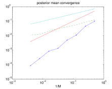
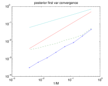
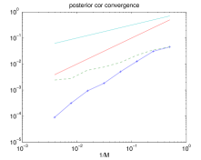
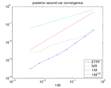
Figure 1: RMSEs of estimates for the posterior mean, variances (var), and correlation (cor) using importance resampling (SIR) and optimal transformations (ETPF) plotted on a log-log scale as a function of ensemble sizes $M$.

We mention that replacing the deterministic transformation step in (47) by drawing ensemble member $j$ from the prior ensemble according to the weights given by the $j$-th column of $S$ leads to a stochastic version of the ETPF. This variant, despite being stochastic like the importance resampling step, results again in a QMC convergence rate.

6 Spatially extended dynamical systems and localization

Let us start this section with a simple thought experiment on the curse of dimensionality. Consider a state space of dimension $N_{z}=100$ and a prior Gaussian distribution with mean zero and covariance matrix $P^{f}=I$. The reference solution is $z_{\rm ref}=0$ and we observe every component of the state vector subject to independent measurement errors with mean zero and variance $R=0.16$. If one applies a single importance resampling step to this problem with ensemble size $M=10$, one finds that the effective sample size collapses to $M_{\rm eff}\approx 1$ and the resulting analysis ensemble is unable to recover the reference solution. However, one also quickly realizes that the stated problem can be decomposed into $N_{z}$ independent data assimilation problems in each component of the state vector alone. If importance resampling is now performed in each component of the state vector independently, then the effective sample size for each of the $N_{z}$ analysis problems remains close to $M=10$ and the reference solution can be recovered from the given set of observations. This is the idea of localization. Note that localization has increased the total sample size to $M\times N_{z}=1000$ for this problem!

We now formally extend LETFs to spatially extended systems which may be viewed as an infinite-dimensional dynamical system (Robinson, 2001) and formulate an appropriate localization strategy. Consider the linear advection equation

$$u_{t}+u_{x}=0$$

as a simple example for such a scenario. If $u_{0}(x)$ denotes the solution at time $t=0$, then

$$u(x,t)=u_{0}(x+t)$$

is the solution of the linear advection equation for all $t\geq 0$. Given a time-increment $\Delta t>0$, the associated dynamical system maps a function $u(x)$ into $u(x+\Delta t)$. A finite-dimensional dynamical system is obtained by discretizing in space with mesh-size $\Delta x>0$. For example, the Box scheme (Morton and Mayers, 2005) leads to

$$\frac{u_{j}^{k+1}+u_{j+1}^{k+1}-u_{j}^{k}-u_{j+1}^{k}}{2\Delta t}+\frac{u_{j+1}^{k+1}+u_{j+1}^{k}-u_{j}^{k+1}-u_{j}^{k}}{2\Delta x}=0$$

and, for $J$ spatial grid points, the state vector at $t_{k}=k\Delta t$ becomes

$$z^{k}=(u_{1}^{k},u_{2}^{k},\ldots,u_{J}^{k})^{T}\in\mathbb{R}^{J}.$$

We may take the formal limit $J\to\infty$ and $\Delta x\to 0$ in order to return to functions $z^{k}(x)$. The dynamical system (6) is then defined as the map that propagates such functions (or their finite-difference approximations) from one observation instance to the next in accordance with the specified numerical method. Here we assume that observations are taken in intervals of $\Delta t_{\rm obs}=N_{\rm out}\Delta t$ with $N_{\rm out}\geq 1$ a fixed integer. The index $n\geq 1$ in (6) is the counter for those observation instances.

In other words, forecast or analysis ensemble members, $z^{f/a}(x)$, now become functions of $x\in\mathbb{R}$, belong to some appropriate function space ${\cal H}$, and the dynamical system (6) is formally replaced by a map or evolution equation on ${\cal H}$ (Robinson, 2001). For simplicity of exposition we assume periodic boundary conditions, i.e., $z(x)=z(x+L)$ for some appropriate $L>0$.

The curse of dimensionality (Bengtsson et al., 2008) implies that, generally speaking, none of the LETFs discussed so far is suitable for data assimilation of spatially extended systems. In order to overcome this situation, we now discuss the concept of localization as first introduced in Houtekamer and Mitchell (2001, 2005) for EnKFs. While we will focus on a particular localization, called R-localization, suggested by Hunt et al. (2007), our methodology can be extended to B-localization as proposed by Hamill et al. (2001).

In the context of the LETFs R-localization amounts to modifying (33) to

$$z^{a}_{j}(x)=\sum_{i=1}^{M}z_{i}^{f}(x)s_{ij}(x),$$

where the associated transform matrices $S(x)\in\mathbb{R}^{M}\times\mathbb{R}^{M}$ depend now on the spatial location $x\in[0,L]$. It is crucial that the transformation matrices $S(x)$ are sufficiently smooth in $x$ in order to produce analysis ensembles with sufficient regularity for the evolution problem under consideration and, in particular $z^{a}_{j}\in{\cal H}$. In case of an SMCM with importance resampling, the resulting $S(x)$ would, in general, not even be continuous for almost all $x\in[0,L)$. Hence we only discuss localization for the ESRF and the ETPF.

Let us, for simplicity, assume that the forward operator $h:{\cal H}\to\mathbb{R}^{N_{y}}$ for the observations $y_{\rm obs}$ is defined by

$$h_{k}(z)=z({\rm x}_{k}),\qquad k=1,\ldots,N_{y}.$$

Here the ${\rm x}_{k}\in[0,L)$ denote the spatial location at which the observation is taken. The measurement errors are Gaussian with mean zero and covariance matrix $R\in\mathbb{R}^{N_{y}\times N_{y}}$. We assume for simplicity that $R$ is diagonal.

In the sequel we assume that $z(x)$ has been extended to $x\in\mathbb{R}$ by periodic extension from $x\in[0,L)$ and introduce time-averaged and normalized spatial correlation function

$$C(x,s):=\frac{\sum_{n=0}^{N}z^{n}(x+s)z^{n}(x)}{\sum_{n=0}^{N}(z^{n}(x))^{2}}$$ (49)

for $x\in[0,L)$ and $s\in[-L/2,L/2)$. Here we have assumed that the underlying solution process is stationary ergodic. In case of spatial homogeneity the spatial correlation function becomes furthermore independent of $x$ for $N$ sufficiently large.

We also introduce a localization kernel ${\cal K}(x,x^{\prime};r_{\rm loc})$ in order to define $R$-localization for an ESRF and the ETPF. The localization kernel can be as simple as

$${\cal K}(x,x;r_{\rm loc})=\left\{\begin{array}[]{ll}1-\frac{1}{2}s&\mbox{for}\,\,s\leq 2,\\ 0&\mbox{else},\end{array}\right.$$ (50)

with

$$s:=\frac{\min\{|x-x^{\prime}-L|,|x-x^{\prime}|,|x-x^{\prime}+L|\}}{r_{\rm loc}}\geq 0,$$

or a higher-order polynomial such as

$${\cal K}(x,x^{\prime};r_{\rm loc})=\left\{\begin{array}[]{ll}1-\frac{5}{3}s^{2}+\frac{5}{8}s^{3}+\frac{1}{2}s^{4}-\frac{1}{4}s^{5}&\mbox{for}\,\,s\leq 1,\\ -\frac{2}{3}s^{-1}+4-5s+\frac{5}{3}s^{2}+\frac{5}{8}s^{3}-\frac{1}{2}s^{4}+\frac{1}{12}s^{5}&\mbox{for}\,\,1\leq s\leq 2,\\ 0&\mbox{else}.\end{array}\right..$$ (51)

See Gaspari and Cohn (1999).

In order to compute the transformation matrix $S(x)$ for given $x$, we modify the $k$th diagonal entry in the measurement error covariance matrix $R\in\mathbb{R}^{N_{y}\times N_{y}}$ and define

$$\frac{1}{\tilde{r}_{kk}(x)}:=\frac{{\cal K}(x,{\rm x}_{k};r_{{\rm loc},R})}{r_{kk}}$$ (52)

for $k=1,\ldots,N_{y}$. Given a localization radius $r_{{\rm loc},R}>0$, this results in a matrix $\tilde{R}^{-1}(x)$ which replaces the $R^{-1}$ in an ESRF and the ETPF.

More specifically, the LETKF is based on the following modifications to the ESRF. First one replaces (43) by

$$Q(x)=\left\{I+\frac{1}{M-1}(A_{y}^{f})^{T}\tilde{R}^{-1}(x)A_{y}^{f}\right\}^{-1}$$

and defines $D(x)=Q(x)^{1/2}$. Finally the localized transformation matrix $S(x)$ is given by

$$s_{ij}(x)=\frac{1}{M-1}q_{ij}(x)(y^{f}_{j}-\bar{y}^{f})\tilde{R}^{-1}(x)(y_{\rm obs}-\bar{y}^{f})+d_{ij}(x),$$ (53)

which replaces (44). We mention that Anderson (2012) discusses practical methods for choosing the localization radius $r_{{\rm loc},R}$ for EnKFs.

In order to extend the concept of $R$-localization to the ETPF, we also define the localized cost function

$$c_{x}(z^{f},z^{a})=\int_{0}^{L}{\cal K}(x,x^{\prime};r_{{\rm loc},c})\|z^{f}(x^{\prime})-z^{a}(x^{\prime})\|^{2}{\rm d}x^{\prime}$$ (54)

with a localization radius $r_{{\rm loc},c}\geq 0$, which can be chosen independently from the localization radius for the measurement error covariance matrix $R$.

The ETPF with R-localization can now be implemented as follows. At each spatial location $x\in[0,L)$ one determines the desired transformation matrix $S(x)$ by first computing the weights

$$w_{i}\propto e^{-\frac{1}{2}(h(z_{i}^{f})-y_{\rm obs})^{T}\tilde{R}^{-1}(x)(h(z_{i}^{f})-y_{\rm obs})}$$ (55)

and then minimizing the cost function

$$J(T)=\sum_{i,j=1}^{M}c_{x}(z_{i}^{f},z_{j}^{f})t_{ij}$$ (56)

over all admissible couplings. One finally sets $S(x)=MT^{\ast}$.

As discussed earlier any infinite-dimensional evolution equation such as the linear advection equation will be truncated in practice to a computational grid $x_{j}=j\Delta x$. The transform matrices $S(x)$ need then to be computed for each grid point only and the integral in (54) is replaced by a simple Riemann sum.

We mention that alternative filtering strategies for spatio-temporal processes have been proposed by Majda and Harlim (2012) in the context of turbulent systems. One of their strategies is to perform localization in spectral space in case of regularly spaced observations. Another spatial localization strategy for particle filters can be found in Rebeschini and van Handel (2013).

7 Applications

In this section we present some numerical results comparing the different LETFs for the chaotic Lorenz-63 (Lorenz, 1963) and Lorenz-96 (Lorenz, 1996) models. While the highly nonlinear Lorenz-63 model can be used to investigate the behavior of different DA algorithms for strongly non-Gaussian distributions, the forty dimensional Lorenz-96 model is a prototype “spatially extended” system which demonstrates the need for localization in order to achieve skillful filter results for moderate ensemble sizes. We begin with the Lorenz-63 model.

We mention that theoretical results on the long time behavior of filtering algorithms for chaotic systems, such as the Lorenz-63 model, have been obtained, for example, by González-Tokman and Hunt (2013) and Law et al. (2013).

7.1 Lorenz-63 model

The Lorenz-63 model is given by the differential equation (7) with state variable $z=({\rm x},{\rm y},{\rm z})^{T}\in\mathbb{R}^{3}$, right hand side

$$f(z) =\left(\begin{array}[]{l}\sigma({\rm y}-{\rm x})\\ {\rm x}(\rho-{\rm z})-{\rm y}\\ {\rm xy}-\beta{\rm z}\end{array}\right),$$

and parameter values $\sigma=10$, $\rho=28$, and $\beta=8/3$. The resulting ODE (7) is discretized in time by the implicit midpoint method (Ascher, 2008), i.e.,

$$z^{n+1}=z^{n}+\Delta tf(z^{n+1/2}),\qquad z^{n+1/2}=\frac{1}{2}(z^{n+1}+z^{n})$$ (57)

with step-size $\Delta t=0.01$. Let us abbreviate the resulting map by $\Psi_{\rm IM}$. Then the dynamical system (6) is defined as

$$\Psi=\Psi_{\rm IM}^{[12]}.$$

In other words observations are assimilated every 12 time-steps. We only observe the ${\rm x}$ variable with a Gaussian measurement error of variance $R=8$.

We used different ensemble sizes from $10$ to $80$ as well as different inflation factors ranging from $1.0$ to $1.12$ by increments of $0.02$ for the EnKF and rejuvenation parameters ranging from $0$ to $0.4$ by increments of $0.04$ for the ETPF. Note that a rejuvenation parameter of $h=0.4$ corresponds to an inflation factor $\alpha=\sqrt{1+h^{2}}\approx 1.0770$.

The following variant of the ETPF with localized cost function has also been implemented. We first compute the importance weights $w_{i}$ of a given observation. Then each component of the state vector is updated using only the distance in that component in the cost function $J(T)$. For example, the ${\rm x}_{i}^{f}$ components of the forecast ensemble members $z_{i}^{f}=({\rm x}_{i}^{f},{\rm y}_{i}^{f},{\rm z}_{i}^{f})^{T}$, $i=1,\ldots,M$, are updated according to

$${\rm x}_{i}^{a}=M\sum_{i=1}^{M}{\rm x}_{i}^{f}t_{ij}^{\ast}$$

with the coefficients $t_{ij}^{\ast}\geq 0$ minimizing the cost function

$$J(T)=\sum_{i,j=1}^{M}t_{ij}|{\rm x}_{i}^{f}-{\rm x}_{j}^{f}|^{2}$$

subject to (36). We use ETPF_R0 as the shorthand form for this method. This variant of the ETPF is of special interest from a computational point of view since the linear transport problem in $\mathbb{R}^{3}$ reduces to three simple one-dimensional problems.

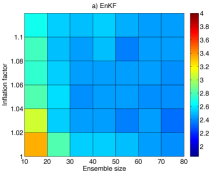
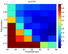
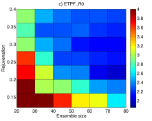
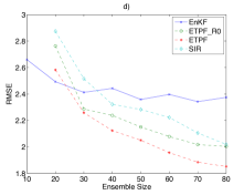
Figure 2: a)-c): Heatmaps showing the RMSEs for different parameters for the EnKF, ETPF and ETPF_R0 for the Lorenz-63 model. d): RMSEs for different ensemble sizes using ’optimal’ inflation factors and rejuvenation.

The model is run over $N=20,000$ assimilation steps after discarding 200 steps to lose the influence of the initial conditions. The resulting root-mean-square errors averaged over time (RMSEs)

$$\text{RMSE}=\frac{1}{N}\sum_{n=1}^{N}\sqrt{\|\bar{z}^{n,a}-z_{\text{ref}}^{n}\|^{2}}$$

are reported in Fig. 2 a)-c). We dropped the results for the ETPF and ETPF_R0 with ensemble size $M=10$ as they indicated strong divergence. We see that the EnKF produces stable results while the other filters are more sensitive to different choices for the rejuvenation parameter. However, with increasing ensemble size and ’optimal’ choice of parameters the ETPF and the ETPF_R0 outperform the EnKF which reflects the biasedness of the EnKF.

Fig. 2 d) shows the RMSEs for each ensemble size using the parameters that yield the lowest RMSE. Here we see again that the stability of the EnKF leads to good results even for very small ensemble sizes. The downside is also evident: While the ETPFs fail to track the reference solution as well as the EnKF for very small ensemble sizes a small increase leads to much lower RMSEs. The asymptotic consistent ETPF outperforms the ETPF_R0 for large ensemble sizes but is less stable otherwise. We also included RMSEs for the SIR filter with rejuvenation parameters chosen from the same range of values as for the ETPFs. Although not shown here, this range seems to cover the ’optimal’ choice for the rejuvenation parameter. The comparison with the EnKF is as expected: for small ensemble sizes the SIR performs worse but beats the EnKF for larger ensemble sizes due to its asymptotic consistency. However, the equally consistent ETPF yields lower RMSEs throughout for the ensemble sizes considered here. Interestingly, the SIR only catches up with the inconsistent but computationally cheap ETPF_R0 for the largest ensemble size in this experiment. We mention that the RMSE drops to around 1.4 with the SIR filter with an ensemble size of 1000.

At this point we note that the computational burden increases considerably for the ETPF for larger ensemble sizes due to the need of solving increasingly large linear transport problems. See the discussion from Section 5.3.

7.2 Lorenz-96 model

Given a periodic domain $x\in[0,L]$ and $N_{z}$ equally spaced grid-points $x_{j}=j\Delta x$, $\Delta x=L/N_{z}$, we denote by $u_{j}$ the approximation to $z(x)$ at the grid points $x_{j}$, $j=1,\ldots,N_{z}$. The following system of differential equations

$$\frac{{\rm d}u_{j}}{{\rm d}t}=-\frac{u_{j-1}u_{j+1}-u_{j-2}u_{j-1}}{3\Delta x}-u_{j}+F,\qquad j=1,\ldots,40,$$ (58)

is due to Lorenz (1996) and is called the Lorenz-96 model. We set $F=8$ and apply periodic boundary conditions $u_{j}=u_{j+40}$. The state variable is defined by $z=(u_{1},\ldots,u_{40})^{T}\in\mathbb{R}^{40}$. The Lorenz-96 model (58) can be seen as a coarse spatial approximation to the PDE

$$\frac{\partial u}{\partial t}=-\frac{1}{2}\frac{\partial(u)^{2}}{\partial x}-u+F,\qquad x\in[0,40/3],$$

with mesh-size $\Delta x=1/3$ and $N_{z}=40$ grid points. The implicit midpoint method (57) is used with a step-size of $\Delta t=0.005$ to discretize the differential equations (58) in time. Observations are assimilated every 22 time-steps and we observe every other grid point with a Gaussian measurement error of variance $R=8$. The large assimilation interval and variance of the measurement error are chosen because of a desired non-Gaussian ensemble distribution.

We used ensemble sizes from 10 to 80, inflation factors from $1.0$ to $1.12$ with increments of $0.02$ for the EnKF and rejuvenation parameters between $0$ and $0.4$ with increments of $0.05$ for the ETPFs.

As mentioned before, localization is required and we take (51) as our localization kernel. For each value of $M$ we fixed a localization radius $r_{{\rm loc},R}$ in (52). The particular choices can be read off of the following table:

M	10	20	30	40	50	60	70	80
$r_{\text{loc},R}^{EnKF}$	2	4	6	6	7	7	8	8
$r_{\text{loc},R}^{ETPF}$	1	2	3	4	5	6	6	6

These values have been found by trial and error and we do not claim that these values are by any means ’optimal’.

As for localization of the cost function (56) for the ETPF we used the same kernel as for the measurement error and implemented different versions of the localized ETPF which differ in the choice of the localization radius: ETPF_R1 corresponds to the choice of $r_{\text{loc},c}=1$ and ETPF_R2 is used for the ETPF with $r_{\text{loc},c}=2$. As before we denote the computationally cheap version with cost function $c_{x_{j}}(z^{f},z^{a})=|u_{j}^{f}-u_{j}^{a}|^{2}$ at grid point $x_{j}$ by ETPF_R0.

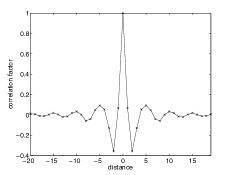
Figure 3: Time averaged spatial correlation between solution components depending on their distance.

The localization kernel as well as the localization radii $r_{\text{loc},c}$ are not chosen by any optimality criterion but rather by convenience and simplicity. A better kernel or localization radii may be derived from looking at the time averaged spatial correlation coefficients (49) as shown in Fig. 3. Our kernel gives higher weights to components closer to the one to be updated, even though the correlation with the immediate neighbor is relatively low.

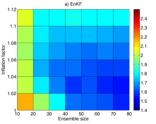
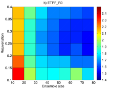
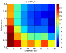
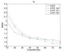
Figure 4: a)-c): Heatmaps showing the RMSEs for different parameters for the EnKF, ETPF_R0 and ETPF_R1 for the Lorenz-96 model. d): RMSEs for different ensemble sizes using ’optimal’ inflation factors and rejuvenation.

The model is run over $N=10,000$ assimilation steps after discarding 500 steps to loose the influence of the initial conditions. The resulting time averaged RMSEs are displayed in Fig. 4. We dropped the results for the smallest rejuvenation parameters as the filters showed strong divergence. Similar to the results for the Lorenz-63 model the EnKF shows the most stable overall performance for various parameters but fails to keep up with the ETPFs for higher ensemble sizes, though the difference between the different filters is much smaller than for the Lorenz-63 system. This is no surprise since the Lorenz-96 system does not have the highly non-linear dynamics of the Lorenz-63 system which causes the involved distributions to be strongly non-Gaussian. The important point here is that the ETPF as a particle filter is able to compete with the EnKF even for small ensemble sizes. Traditionally, high dimensional systems required very high ensemble sizes for particle filters to perform reasonably well. Hundreds of particles are necessary for the SIR to be even close to the true state.

8 Historical comments

The notion of data assimilation has been coined in the field of meteorology and more widely in the geosciences to collectively denote techniques for combining computational models and physical observations in order to estimate the current state of the atmosphere or any other geophysical process. The perhaps first occurrence of the concept of data assimilation can be found in the work of Richardson (1922), where observational data needed to be interpolated onto a grid in order to initialize the computational forecast process. With the rapid increase in computational resolution starting in the 1960s, it became quickly necessary to replace simple data interpolation by an optimal combination of first guess estimates and observations. This gave rise to techniques such as the successive correction method, nudging, optimal interpolation and variational least square techniques (3D-Var and 4D-Var). See Daley (1993); Kalnay (2002) for more details.

Leith (1974) proposed ensemble (or Monte Carlo) forecasting as an alternative to conventional single forecasts. However ensemble forecasting did not become operational before 1993 due to limited computer resources (Kalnay, 2002). The availability of ensemble forecasts subsequently lead to the invention of the EnKF by Evensen (1994) with a later correction by Burgers et al. (1998) and many subsequent developments, which have been summarized in Evensen (2006). We mention that the analysis step of an EnKF with perturbed observations is closely related to a method now called randomized likelihood method (Kitanidis, 1995; Oliver, 1996; Oliver et al., 1996).

In a completely independent line of research the problem of optimal estimation of stochastic processes from data has led to the theory of filtering and smoothing, which started with the work of Wiener (1948). The state space approach to filtering of linear systems gave rise to the celebrated Kalman filter and more generally to the stochastic PDE formulations of Zakai and Kushner-Stratonovitch in case of continuous-time filtering. See Jazwinski (1970) for the theoretical developments up to 1970. Monte Carlo techniques were first introduced to the filtering problem by Handschin and Mayne (1969), but it was not until the work of Gordon et al. (1993) that the SMCM became widely used (Doucet et al., 2001). The McKean interacting particle approach to SMCMs has been pioneered by del Moral (2004). The theory of particle filters for time-continuous filtering problems is summarized in Bain and Crisan (2009).

Standard SMCMs suffer from the curse of dimensionality in that the necessary number of ensemble members $M$ increases exponentially with the dimension $N_{z}$ of state space (Bengtsson et al., 2008). This limitation has prevented SMCMs from being used in meteorology and the geosciences. On the other hand, it is known that EnKFs lead to inconsistent estimates which is problematic when multimodal forecast distributions are to be expected. Current research work is therefore focused on a theoretical understanding of EnKFs and related sequential assimilation techniques (see, for example, González-Tokman and Hunt (2013); Law et al. (2013)), extensions of particle filters/SMCMs to PDE models (see, for example, Morzfeld and Chorin (2012); van Leeuwen and Ades (2012); Beskov et al. (2013); Metref et al. (2013)), and Bayesian inference on function spaces (see, for example, Stuart (2010); Cotter et al. (2009); Dashti et al. (2013)) and hybrid variational methods such as by, for example, Bonavita et al. (2012); Clayton et al. (2013).

A historical account of optimal transportation can be found in Villani (2009). The work of McCann (1995) provides the theoretical link between the classic linear assignment problem and the Monge-Kantorovitch problem of coupling PDFs. The ETPF is a computational procedure for approximating such couplings using importance sampling and linear transport instead.

9 Summary and Outlook

We have discussed various ensemble/particle-based algorithms for sequential data assimilation in the context of LETFs. Our starting point was the McKean interpretation of Feynman-Kac formulae. The McKean approach requires a coupling of measures which can be discussed in the context of optimal transportation. This approach leads to the ETPF when applied in the context of SMCMs. We have furthermore discussed extensions of LETFs to spatially extended systems in form of $R$-localization.

The presented work can be continued along several lines. First, one may replace the empirical forecast measure

$$\pi_{\rm emp}^{f}(z):=\frac{1}{M}\sum_{i=1}^{M}\delta(z-z_{i}^{f}),$$ (59)

which forms the basis of SMCMs and the ETPF, by a Gaussian mixture

$$\pi_{\rm GM}^{f}(z):=\frac{1}{M}\sum_{i=1}^{M}{\rm n}(z;z_{i}^{f},B),$$ (60)

where $B\in\mathbb{R}^{N_{z}\times N_{z}}$ is a given covariance matrix and

$${\rm n}(z;m,B):=\frac{1}{(2\pi)^{N_{z}/2}|B|^{1/2}}e^{-\frac{1}{2}(z-m)^{T}B^{-1}(z-m)}.$$

Note that the empirical measure (59) is recovered in the limit $B\to 0$. While the weighted empirical measure

$$\pi_{\rm emp}^{a}(z):=\sum_{i=1}^{M}w_{i}\delta(z-z_{i}^{f})$$

with weights given by (35) provides the analysis in case of an empirical forecast measure (59) and an observation $y_{\rm obs}$, a Gaussian mixture forecast PDF (60) leads to an analysis PDF in form of a weighted Gaussian mixture provided the forward operator $h(z)$ is linear in $z$. This fact allows one to extend the ETPF to Gaussian mixtures. See Reich and Cotter (2015) for more details. Alternative implementations of Gaussian mixture filters can, for example, be found in Stordal et al. (2011) and Frei and Künsch (2013).

Second, one may factorize the likelihood function $\pi_{Y^{1:N}}(y^{1:N}|z^{0,N})$ into $L>1$ identical copies

$$\hat{\pi}_{Y^{1:N}}(y^{1:N}|z^{0:N}):=\frac{1}{(2\pi)^{N_{y}N/2}|R/L|^{N/2}}\prod_{n=1}^{N}e^{-\frac{1}{2L}(h(z^{n})-y^{n})^{T}R^{-1}(h(z^{n})-y^{n})},$$

i.e.,

$$\pi_{Y^{1:N}}(y^{1:N}|z^{0,N})=\prod_{l=1}^{L}\hat{\pi}_{Y^{1:N}}(y^{1:N}|z^{0:N})$$

and one obtains a sequence of $L$ “incremental” Feynman-Kac formulae. Each of these formulae can be approximated numerically by any of the methods discussed in this review. For example, one obtains the continuous EnKF formulation of Bergemann and Reich (2010) in the limit $L\to\infty$ in case of an ESRF. We also mention the continuous Gaussian mixture ensemble transform filter (Reich, 2012). An important advantage of an incremental approach is the fact that the associated weights (35) remain closer to the uniform reference value $1/M$ in each iteration step. See also related methods such as running in place (RIP) (Kalnay and Yang, 2010), the iterative EnKF approach of Bocquet and Sakov (2012); Sakov et al. (2012), and the embedding approach of Beskov et al. (2013) for SMCMs.

Third, while this paper has been focused on discrete time algorithms, most of the presented results can be extended to differential equations with observations arriving continuously in time such as

$${\rm d}y_{\rm obs}(t)=h(z_{\rm ref}(t)){\rm d}t+\sigma{\rm d}W(t),$$

where $W(t)$ denotes standard Brownian motion and $\sigma>0$ determines the amplitude of the measurement error. The associated marginal densities satisfy the Kushner-Stratonovitch stochastic PDE (Jazwinski, 1970). Extensions of the McKean approach to continuous-in-time filtering problems can be found in Crisan and Xiong (2010) and Yang et al. (2013). We also mention the continuous-in-time formulation of the EnKF by Bergemann and Reich (2012). More generally, a reformulation of LETFs in terms of continuously-in-time arriving observations is of the abstract form

$${\rm d}z_{j}=f(z_{j}){\rm d}t+\sum_{i=1}^{M}z_{i}{\rm d}s_{ij},\qquad j=1,\ldots,M.$$ (61)

Here $S(t)=\{s_{ij}(t)\}$ denotes a matrix-valued stochastic process which depends on the ensemble $\{z_{i}(t)\}$ and the observations $y_{\rm obs}(t)$. In other words, (61) leads to a particular class of interacting particle systems and we leave further investigations of its properties for future research. We only mention that the continuous-in-time EnKF formulation of Bergemann and Reich (2012) leads to

$${\rm d}s_{ij}=\frac{1}{M-1}(y_{i}-\bar{y})\sigma^{-1}({\rm d}y_{\rm obs}-y_{j}{\rm d}t+\sigma^{1/2}{\rm d}W_{j}),$$

where the $W_{j}(t)$’s denote standard Brownian motion, $y_{j}=h(z_{j})$, and $\bar{y}=\frac{1}{M}\sum_{i=1}^{M}y_{i}$. See als Amezcua et al. (2014) for related reformulations of ESRFs.