$Y(3940)$ as a Mixed Charmonium-Molecule State

Abstract

Using the QCD sum rules approach we study the mass and decay width of the channel $J/\psi\>\omega$ for the $Y(3940)$ state, assuming that it can be described by a mixed charmonium-molecule scalar state $(\chi_{c0})\!-\!(D^{\ast}\!\bar{D}^{\ast})$ current with $J^{PC}=0^{++}$ quantum numbers. For the mixing angle $\theta=(76.0\pm 5.0)^{\circ}$, we obtain the value $M_{Y}=(3.95\pm 0.11)~{}\mbox{GeV}$ for the mass, which is in good agreement with the experimental mass of the $Y(3940)$ state. For the decay width into the channel $Y\to J/\psi\>\omega$ we find the value $\Gamma_{Y\to J/\psi\>\omega}=(1.7\pm 0.6)\nobreak\,\mbox{MeV}$, which is also compatible with the experimental data. We thus conclude that the present description of the $Y(3940)$ as a mixed charmonium-molecule state is a possible scenario to explain the structure of this state.

I Introduction

In the past years several states in the region of mass of about 3940 MeV has been observed in different processes of production and decay. The state $X(3915)$ was observed by Belle Collaboration in the process $\gamma\gamma\to\,J/\psi\,\omega$ belleX3915 , with a mass $m=(3915\pm 3\pm 2)$ MeV and total width $\Gamma=(17\pm 10\pm 3)$ MeV. In addition, the observation of the state $Y(3940)$ has been made by Belle Collaboration in the decay $B\to(J/\psi\,\omega)K$, with a mass $m=3943\pm 11({\mbox{{\it stat}}})\pm 13({\mbox{{\it syst}}})$ MeV and decay width $\Gamma=87\pm 22({\mbox{\it stat}})\pm 26({\mbox{\it syst}})$ MeV belleY3940 . Afterwards, this state has been also observed in the process $B\to(J/\psi\,\omega)K$ by Babar Collaboration, with a slightly smaller mass of $m=3914.6^{+3.9}_{-3.4}~{}({\mbox{{\it stat}}})~{}\pm~{}2.0({\mbox{\it syst}})$ MeV and width $\Gamma=34^{+12}_{-8}~{}({\mbox{{\it stat}}})~{}\pm~{}5.0({\mbox{\it syst}})$ MeV babarY3940 . In the same mass region, the state $Z(3930)$ was discovered in the process $\gamma\gamma\to\,D\bar{D}$, that is generally linked to the charmonium state $\chi_{c2}(2P)$ belleZ3940 ; babarZ3940 .

The proximity of the masses could indicate that all these states are connected to the same particle observed in different processes. There are evidences, however, that the two reported states, $Y(3940)$ and $X(3915)$, could be interpreted as molecular states. The $X(3915)$ state has a larger product of the two-photon width times the decay branching fraction than usually expected for charmonium states, as noted in Ref. babar2 . Regarding the $Y(3940)$, the lower limit for the decay channel $J/\psi\>\omega$ has been estimated to be $\Gamma>1$ MeV, which is large for a channel that is OZI suppressed for conventional charmonium states godfrey ; godfrey2 . These facts suggests that these states cannot be interpreted as a conventional $c\bar{c}$ state. In Ref. liu , it was proposed that the $Y(3940)$ can be a molecular state $D^{*}\bar{D}^{*}$, with quantum numbers $J^{PC}=0^{++}$ or $2^{++}$. It was also concluded that the $Y(3940)$ must be the molecular partner of the state $Y(4140)$, a $D^{*}_{s}\bar{D}^{*}_{s}$ molecule. This interpretation has been tested in several approaches, such as phenomenological lagrangians gutsche and vector-meson dominance oset . In Ref. albuquerque , the $Y$ state was studied with QCD Sum Rules (QCDSR) method svz ; rry ; SNB as a $D^{*}\bar{D}^{*}$ molecule with quantum numbers $0^{++}$ and the mass obtained was $m_{D^{*}\bar{D}^{*}}=(4.13\pm 0.10)$ MeV, failing to reproduce the experimental mass of the state.

In the present work we revisit the study of the $Y(3940)$ within QCDSR approach, using a mixed charmonium-molecule current. The prescription of a mixture of two- and four-quarks states has been successfully implemented for other states in the framework of sum rules. Following the work of Ref. oka that was applied in the light quark sector, the authors in Refs. matheusX3872 ; x3872rad ; x3872prod described the $X(3872)$ state as a molecule-charmonium state, implementing the mixing of the current and extending it to the charm sector. In these works the mass and decay width for the channels $J/\psi+(2\pi,3\pi,\gamma)$ and the production in $B$-meson decays were estimated in a good agreement with the experimental values. Another state that was studied as a mixture was the $Y(4260)$. In Ref. diasY4260 , the $Y(4260)$ was described as a tetraquark-charmonium mixed state, and the mass and decay width estimated are also consistent with the experimental values.

In the following sections we use the QCDSR approach to describe the $Y(3940)$ as a mixing between the $\chi_{c0}$ charmonium and the $D^{\ast}\!\bar{D}^{\ast}$ molecule, with $J^{PC}=0^{++}$. We obtain the mass for this state and the decay width in the channel $Y\to J/\psi\>\omega$.

II Mixed Hadronic Current

In order to evaluate the sum rule for the $Y(3940)$ state as a mixed $(\chi_{c0})\!-\!(D^{\ast}\!\bar{D}^{\ast})$ state, with $J^{PC}=0^{++}$, one employs the following hadronic current

$$j = a\>\mbox{cos}\>\theta~{}j_{{}_{\chi_{c0}}}~{}+~{}\mbox{sin}\>\theta~{}j_{{}_{D^{\ast}\!D^{\ast}}}$$ (1)

where $\theta$ is an arbitrary mixing angle. The meson and molecule currents are, respectively, given by:

$$j_{{}_{\chi_{c0}}} = \bar{c}_{k}c_{k}$$ (2)

$$j_{{}_{D^{\ast}\!D^{\ast}}} = \left(\bar{q}_{i}\gamma_{\mu}c_{i}\right)\left(\bar{c}_{j}\gamma^{\mu}q_{j}\right)~{}~{}.$$ (3)

Notice that the normalization factor $a$ is introduced in Eq. (1) for ensuring that the mixed current can be evaluated at the same Fock space. Usually, one sets oka ; matheusX3872 ; x3872rad ; x3872prod

$$a=-\frac{\langle\bar{q}q\rangle}{\sqrt{2}}~{}.$$ (4)

Then, evaluating the two- and three-point correlation functions altogether with Eq. (1) one can estimate the mass and decay width of the mixed $(\chi_{c0})\!-\!(D^{\ast}\!\bar{D}^{\ast})$ state.

III Two-Point Correlation Function

To obtain the mass of a hadronic state using the QCDSR approach, one has to evaluate the two-point correlation function

$$\Pi(q) = i\int d^{4}x~{}e^{iq\cdot x}\langle 0|\>T[j(x)j^{\dagger}(0)]\>|0\rangle$$ (5)

According to the quark-hadron duality principle, Eq. (5) can be evaluated in two ways: the phenomenological side and the QCD side. The phenomenological side is calculated by inserting, in Eq. (5), a complete set of intermediate states, $Y$, which couple to the hadronic current in Eq. (1). Parametrizing this coupling through a generic parameter $\lambda_{Y}$, one defines

$$\langle 0|\>j\>|Y\rangle=\lambda_{Y}~{}.$$ (6)

Using Eq. (6) and after some algebraic manipulation, one can write the phenomenological side of Eq. (5) as

$$\Pi^{\mbox{\tiny$PHEN$}}(q)=\frac{\lambda_{Y}^{2}}{M_{Y}^{2}-q^{2}}+\int\limits_{0}^{\infty}\!ds\>\frac{\rho^{\mbox{\tiny$cont$}}(s)}{s-q^{2}}$$ (7)

where $M_{Y}$ is the mixed $(\chi_{c0})\!-\!(D^{\ast}\!\bar{D}^{\ast})$ ground state mass and the second term in the RHS of Eq. (7) denotes the continuum (or higher resonance) contributions. As usual in a QCDSR approach, it is assumed that the continuum contribution to the spectral density, $\rho^{\mbox{\tiny$cont$}}(s)$ in Eq. (7), vanishes below a certain threshold $s_{0}$. Above this threshold, it is assumed that the result coincides with the one obtained in the OPE side. Therefore, one uses the ansatz io1

$$\rho^{\mbox{\tiny$cont$}}(s) = \rho^{\mbox{\tiny$OPE$}}(s)\>\Theta(s-s_{0})$$ (8)

where $\Theta(s-s_{0})$ is the Heaviside step function.

In the OPE side, one calculates the correlation function in terms of quark and gluon fields using the Wilson’s operator product expansion (OPE). This is also called the OPE side. Then, inserting Eq. (1) into the above equation, one obtains

$$\Pi^{\mbox{\tiny$OPE$}}(q) = i\!\int\!\!d^{4}x\,e^{iq\cdot x}\Bigg{\{}\!\frac{1}{2}\langle\bar{q}q\rangle^{2}\mbox{cos}^{2}\theta~{}\Pi_{{}_{\chi_{c0}}}+\mbox{sin}^{2}\theta~{}\Pi_{{}_{D^{\ast}\!D^{\ast}}}$$ (9)

$$-~{}\frac{\langle\bar{q}q\rangle}{\sqrt{2}}\>\mbox{sin}\,\theta\>\mbox{cos}\,\theta~{}\Big{[}\Pi_{{}_{mix}}+\Pi_{{}_{mix}}^{\ast}\Big{]}\Bigg{\}}$$

where the $\Pi_{{}_{\chi_{c0}}}(x)$ and $\Pi_{{}_{D^{\ast}\!D^{\ast}}}(x)$ functions are, respectively, the correlation functions of the $\chi_{c0}$ meson and the $D^{\ast}D^{\ast}~{}(0^{++})$ molecular state, which have been calculated in other works albuquerque ; rry . Thus, one only has to calculate the $\Pi_{{}_{mix}}(x)$ and $\Pi_{{}_{mix}}^{\ast}(x)$ functions defined as follows:

$$\Pi_{{}_{mix}}(x) = \langle 0|\>T[j_{{}_{\chi_{c0}}}(x)j_{{}_{D^{\ast}\!D^{\ast}}}^{\dagger}(0)]\>|0\rangle$$ (10)

$$= -\mbox{Tr}\bigg{[}S^{q}_{ji}(0)\>\gamma_{\mu}\>S^{c}_{ik}(-x)S^{c}_{kj}(x)\>\gamma^{\mu}\bigg{]}$$

$$\Pi_{{}_{mix}}^{\ast}(x) = \langle 0|\>T[j_{{}_{D^{\ast}\!D^{\ast}}}(x)j_{{}_{\chi_{c0}}}^{\dagger}(0)]\>|0\rangle$$ (11)

$$= -\mbox{Tr}\bigg{[}S^{q}_{ji}(0)\>\gamma_{\mu}\>S^{c}_{ik}(x)S^{c}_{kj}(-x)\>\gamma^{\mu}\bigg{]}$$

where $S^{c}(x)$ and $S^{q}(x)$ are the charm- and light-quark propagators, respectively. The next step is to write the correlation function in terms of a dispersion relation, such that

$$\Pi^{\mbox{\tiny$OPE$}}(q^{2})=\int\limits_{4m^{2}_{c}}^{\infty}\!ds\>\frac{\rho^{\mbox{\tiny$OPE$}}(s)}{s-q^{2}},$$ (12)

where $\rho^{\mbox{\tiny$OPE$}}(s)$ is given by the imaginary part of the correlation function: $\pi\>\rho^{\mbox{\tiny$OPE$}}(s)=\mbox{Im}[\>\Pi^{\mbox{\tiny$OPE$}}(q^{2}=s)\>]$. According to Eq. (9), the expression for the spectral density is

$$\rho^{\mbox{\tiny$OPE$}}(s) = \!\frac{1}{2}\langle\bar{q}q\rangle^{2}\mbox{cos}^{2}\theta~{}\rho_{{}_{\chi_{c0}}}(s)+\mbox{sin}^{2}\theta~{}\rho_{{}_{D^{\ast}\!D^{\ast}}}(s)$$ (13)

$$-~{}\frac{\langle\bar{q}q\rangle}{\sqrt{2}}\>\mbox{sin}\,\theta\>\mbox{cos}\,\theta~{}\rho_{{}_{mix}}(s)~{}~{}.$$

One calculates the sum rule at leading order in $\alpha_{s}$ in the operators and considers the contributions from the condensates up to dimension-8 in the OPE. The expressions for the spectral density are given in Appendix A.

To improve the matching between the two sides of the sum rule, one performs the Borel transform. After transferring the continuum contributions to the OPE side, the sum rule for the scalar charmonium-molecule, considered as a mixed scalar $(\chi_{c0})\!-\!(D^{\ast}\!\bar{D}^{\ast})$ state, can be written as

$$\lambda_{Y}^{2}\>e^{-{M_{Y}^{2}}/M_{B}^{2}} =\int\limits^{s_{0}}_{4m_{c}^{2}}\!\!ds\>e^{-s/M_{B}^{2}}~{}\rho^{\mbox{\tiny$OPE$}}(s)~{}~{}.$$ (14)

Therefore, one can estimate the ground state mass from the following ratio

$${\cal R}=\frac{\int\limits_{4m_{c}^{2}}^{s_{0}}\!\!ds\>s\>e^{-s/M_{B}^{2}}~{}\rho^{\mbox{\tiny$OPE$}}(s)}{\int\limits_{4m_{c}^{2}}^{s_{0}}\!\!ds\>e^{-s/M_{B}^{2}}~{}\rho^{\mbox{\tiny$OPE$}}(s)}$$ (15)

where at the $M_{B}^{2}$-stability point, one obtains

$$M_{Y} \simeq \sqrt{{\cal R}}~{}~{}.$$ (16)

III.1 Numerical Analysis

The numerical values for the quark masses and condensates are listed in Table 1. These values are consistent with the ones used in Refs. x3872rad ; x3872prod ; diasY4260 for the QCDSR analysis on other mixed hadronic states.

Table 1: QCD input parameters.

Parameters	Values
$\overline{m}_{c}$	$(1.23-1.47)\nobreak\,\mbox{GeV}$
$\langle\bar{q}q\rangle$	$-(0.23\pm 0.03)^{3}\nobreak\,\mbox{GeV}^{3}$
$\langle g_{s}^{2}G^{2}\rangle$	$(0.88\pm 0.25)~{}\nobreak\,\mbox{GeV}^{4}$
$\langle g_{s}^{3}G^{3}\rangle$	$(0.58\pm 0.18)~{}\nobreak\,\mbox{GeV}^{6}$
$m_{0}^{2}\equiv\langle\bar{q}Gq\rangle/\langle\bar{q}q\rangle$	$(0.8\pm 0.1)~{}\nobreak\,\mbox{GeV}^{2}$
$\rho\equiv\langle\bar{q}q\bar{q}q\rangle/\langle\bar{q}q\rangle^{2}$	$(0.5-2.0)$

For reliable results in a sum rule calculation, one must establish a valid Borel window which guarantees the existence of a region with $M_{B}^{2}$-stability, a good OPE convergence and pole dominance over continuum contributions. Nevertheless, another crucial point is the optimal choice of the continuum threshold $s_{0}$ and the mixing angle $\theta$.

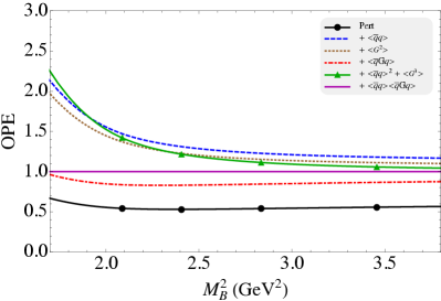
Figure 1: OPE convergence in the region $1.7\leq M_{B}^{2}\leq 3.8~{}\nobreak\,\mbox{GeV}^{2}$ for $\sqrt{s_{0}}=4.40\nobreak\,\mbox{GeV}$ and $\theta=76.0^{\circ}$. One plots the relative contributions starting with the perturbative contribution (line with circles), and each other line represents the relative contribution after adding of one extra condensate in the expansion: + $\langle\bar{q}q\rangle$ (dashed line), + $\langle G^{2}\rangle$ (dotted line), + $\langle\bar{q}Gq\rangle$ (dot-dashed line), + $\langle\bar{q}q\rangle^{2}$ + $\langle G^{3}\rangle$ (line with triangles) and $\langle\bar{q}q\rangle\cdot\langle\bar{q}Gq\rangle$ (solid line).

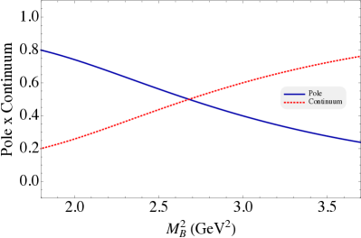
Figure 2: The pole (solid line) and continuum (dotted line) contributions for $\sqrt{s_{0}}=4.40\nobreak\,\mbox{GeV}$ and $\theta=76.0^{\circ}$.

We start our analysis discussing the possible values of both parameters. Considering that we are interested in a mixed state with a mass $M_{Y}\!\sim\!3.9\nobreak\,\mbox{GeV}$, a reasonable initial value for the continuum threshold would be $\sqrt{s_{0}}=4.40\nobreak\,\mbox{GeV}$. In principle, the choice of the mixing angle seems to be arbitrary. Hence, for a fixed value of $\theta$, we search for a continuum threshold which allows us to determine the best $M_{B}^{2}$-stability inside of a valid Borel window. After lengthy numerical calculations, we find that the optimal choice is

$$\sqrt{s_{0}} = (4.40\pm 0.10)\nobreak\,\mbox{GeV}$$ (17)

$$\theta = (76.0\pm 5.0)^{\circ}~{}~{}.$$ (18)

We notice that the OPE does not converge for $\theta$ values outside this range. Using these values, we analyze the relative contributions of the terms in the OPE, for $\sqrt{s_{0}}=4.40\nobreak\,\mbox{GeV}$ and $\theta=76.0^{\circ}$. As one can see in Fig. 1, the contribution of the dimension-8 condensate is smaller than $20$% of the total contribution for values of $M_{B}^{2}\geq 2.4\nobreak\,\mbox{GeV}^{2}$, which indicates the starting point for a good OPE convergence. In order to determine the maximum value of the Borel mass parameter, we must analyze the pole contribution. Since the QCDSR approach extracts information only from the ground state, we have to ensure that the pole contribution is greater than the continuum contribution. Thus, we fix the maximum value of the Borel mass parameter as the value for which the pole is greater than or equal to the continuum contribution. From Fig. 2, we can see that this condition is satisfied when $M_{B}^{2}=2.7\nobreak\,\mbox{GeV}^{2}$. Therefore, the Borel window is set as $2.4\leq M^{2}_{B}\leq 2.7$ GeV².

In Fig. 3, we plot the ground state mass as a function of $M_{B}^{2}$, considering three different values of $\sqrt{s_{0}}$. We conclude that there is a good $M_{B}^{2}$-stability in the determined Borel window.

Varying the value of the continuum threshold in the range $\sqrt{s_{0}}=(4.40\pm 0.10)\nobreak\,\mbox{GeV}$, the mixing angle in the range $\theta=(76.0\pm 5.0)^{\circ}$, and the other parameters as indicated in Table 1, we get

$$M_{Y}=(3.95\pm 0.11)~{}\mbox{GeV}~{}.$$ (19)

This mass is compatible with the experimental mass of the $Y(3940)$ state observed by Belle Collaboration belleY3940 . Therefore, from a QCD sum rule point of view, a mixed scalar $(\chi_{c0})\!-\!(D^{\ast}\!\bar{D}^{\ast})$ state could be a good candidate to explain the $Y(3940)$ state.

After the determination of the mass, we can use this result in Eq. (14) to estimate the coupling parameter, defined in Eq. (6). Therefore, considering the same values of $s_{0}$, $\theta$ and the Borel window used for the mass calculation, we obtain

$$\lambda_{Y}=(2.1\pm 0.6)\times 10^{-2}~{}\mbox{GeV}^{5}.$$ (20)

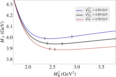
Figure 3: The mass as a function of the sum rule parameter $M_{B}^{2}$ for $\sqrt{s_{0}}=4.30\nobreak\,\mbox{GeV}$ (dotted line), $\sqrt{s_{0}}=4.40\nobreak\,\mbox{GeV}$ (solid line) and $\sqrt{s_{0}}=4.50\nobreak\,\mbox{GeV}$ (dashed line). The respective parentheses indicate the valid Borel window.

IV The $Y(3940)\to J/\psi\>\omega$ decay width

In order to provide more evidence to support the conclusion reached at the end of the previous section, that the $Y(3940)$ can be explained as a scalar mixed state, we now use the QCDSR to compute the form factor associated with the vertex $Y\>J/\psi\>\omega$ and to estimate the width of the channel $Y(3940)\to J/\psi\>\omega$. For this purpose, we start writing the three-point function defined as

$$\Pi_{\mu\nu}(p,p^{\prime},q)=\int d^{4}x\>d^{4}y~{}e^{ip^{\prime}\cdot x}\>e^{iq\cdot y}~{}\Pi_{\mu\nu}(x,y),$$ (21)

where $p=p^{\prime}+q$ and $\Pi_{\mu\nu}(x,y)$ is given by

$$\Pi_{\mu\nu}(x,y)=\langle 0|T\{j_{\mu}^{\psi}(x)j_{\nu}^{\omega}(y)j^{\dagger}(0)\}|0\rangle.$$ (22)

The interpolating currents for the $J/\psi$ meson and the mixed $(\chi_{c0})\!-\!(D^{\ast}\!\bar{D}^{\ast})$ state used in Eq. (22) are defined in Section II, while the interpolating current associated with the $\omega$ meson is defined by

$$j^{\omega}_{\nu}=\frac{1}{6}\Big{(}\bar{u}_{a}\gamma_{\nu}u_{a}+\bar{d}_{a}\gamma_{\nu}d_{a}\Big{)}.$$ (23)

In the same manner that it was done for the two-point correlation function, we again invoke the quark-hadron duality principle to calculate the three-point function in two ways. We match both sides after performing the Borel transform. In the phenomenological side, one has to insert the intermediate states for the $J/\psi$, $\omega$ and $Y(3940)$ mesons in Eq. (21). Using the following relations:

$$\langle 0|\>j_{\mu}^{\psi}\>|J/\psi(p^{\prime})\rangle = M_{\psi}f_{\psi}\>\epsilon_{\mu}(p^{\prime}),$$

$$\langle 0|\>j^{\omega}_{\nu}\>|\omega(q)\rangle = M_{\omega}f_{\omega}\>\epsilon_{\nu}(q),$$ (24)

$$\langle Y(p)|\>j\>|0\rangle = \lambda_{Y},$$

we obtain the expression

$$\Pi_{\mu\nu}^{\mbox{\tiny$PHEN$}}(p,p^{\prime},q) = {\lambda_{Y}\>M_{\psi}f_{\psi}\>M_{\omega}f_{\omega}~{}g_{{}_{\!Y\!\psi\omega}}(q^{2})\over(p^{2}-M_{Y}^{2})({p^{\prime}}^{2}-M_{\psi}^{2})(q^{2}-M_{\omega}^{2})}~{}~{}$$ (25)

$$\times~{}\Big{[}q_{\mu}p^{\prime}_{\nu}-(p^{\prime}\cdot q)g_{\mu\nu}\Big{]}+\cdots\;,$$

where the dots stand for the contribution of all possible excited states. The form factor, $g_{{}_{\!Y\!\psi\omega}}(q^{2})$, is defined by the generalization of the on-shell mass matrix element, $\langle J/\psi\>\omega\>|\>Y\rangle$, for an off-shell $\omega$ meson:

$$\langle J/\psi\>\omega\>|\>Y\rangle = g_{{}_{\!Y\!\psi\omega}}(q^{2})\bigg{[}\Big{(}p^{\prime}\cdot\epsilon^{*}(q)\Big{)}\Big{(}q\cdot\epsilon^{*}(p^{\prime})\Big{)}$$ (26)

$$-~{}(p^{\prime}\cdot q)\Big{(}\epsilon^{*}(p^{\prime})\cdot\epsilon^{*}(q)\Big{)}\bigg{]},$$

which can be extracted from the effective Lagrangian that describes the coupling between two vector mesons and one scalar meson:

$${\cal{L}}=\frac{i}{2}\>g_{{}_{\!Y\!\psi\omega}}V_{\alpha\beta}\Psi^{\alpha\beta}~{}Y$$ (27)

where $V_{\alpha\beta}=\partial_{\alpha}\omega_{\beta}-\partial_{\beta}\omega_{\alpha}$ and $\Psi^{\alpha\beta}=\partial^{\alpha}\psi^{\beta}-\partial^{\beta}\psi^{\alpha}$, are the tensor fields of the $\omega$ and $\psi$ fields respectively.

In the OPE side, we calculate the correlation function at leading order in $\alpha_{s}$ and we consider condensates up to dimension 7. Notice that the three-point function includes a number of different Lorentz structures and the most suitable one for our purposes seems to be the $q_{\mu}p^{\prime}_{\nu}$. The reasons for the choice of this structure are: (a) it has the larger number of momenta; (b) the OPE leading term decreases as $1/Q^{2}$ as $Q^{2}\rightarrow\infty$, which is an expected behavior for QCD form factors. In general, for any given structure, the sum rule method is inapplicable at large $Q^{2}$ where the power corrections become large and uncontrollable. At small $Q^{2}$, the situation is even worse since when approaching the physical region the operator expansion stops working. In this sense, one has to consider that the sum rule is valid up to a rather small $Q^{2}$ and the extrapolation from the values of $Q^{2}$ to the physical region can be obtained with a good accuracy.

Matching both side of the sum rule, taking the approximation $p^{2}\simeq{p^{\prime}}^{2}=-P^{2}$ and doing the Borel transform to $P^{2}\rightarrow M_{B}^{2}$, we get the following expression in the $q_{\mu}p^{\prime}_{\nu}$ structure:

$$\frac{\lambda_{Y}M_{\omega}f_{\omega}M_{\psi}f_{\psi}~{}g_{{}_{\!Y\!\psi\omega}}(Q^{2})}{(M_{Y}^{2}-M_{\psi}^{2})(Q^{2}+M_{\omega}^{2})}\!\!\!\!\!\!\! \>\left(e^{-M_{Y}^{2}/M_{B}^{2}}-e^{-M_{\psi}^{2}/M_{B}^{2}}\right)+$$

$$+H(Q^{2})~{}e^{-s_{0}/M_{B}^{2}} = \Pi^{\mbox{\tiny$OPE$}}(M_{B}^{2},Q^{2}),$$ (28)

where $Q^{2}=-q^{2}$, and $H(Q^{2})$ function represents the contribution to the pole-continuum transitions matheusX3872 ; io2 ; decayx ; dsdpi . The $\Pi^{\mbox{\tiny$OPE$}}(M_{B}^{2},Q^{2})$ function is

$$\Pi^{{\mbox{\tiny$OPE$}}}(M_{B}^{2},Q^{2})=\sin\theta\int\limits_{4m_{c}^{2}}^{+\infty}\!\!ds~{}e^{-s/M_{B}^{2}}\>\rho(s,Q^{2})~{},$$ (29)

and $\rho=\rho^{pert}+\rho^{\langle\bar{q}q\rangle}+\rho^{\langle G^{2}\rangle}+\rho^{\langle\bar{q}Gq\rangle}+\rho^{\langle\bar{q}q\rangle\langle G^{2}\rangle}$ is given explicitly by

$$\rho^{pert}(s,Q^{2}) = ~{}~{}\rho^{\langle\bar{q}q\rangle}(s,Q^{2})~{}~{}=~{}~{}0~{},$$ (30)

$$\rho^{\langle G^{2}\rangle}(s,Q^{2}) = -\frac{\langle g_{s}^{2}G^{2}\rangle}{3^{2}\cdot 2^{10}\>\pi^{4}}\int\limits_{0}^{1}\!d\alpha~{}\delta\!\left[s-\frac{m_{c}^{2}}{\alpha(1\!-\!\alpha)}\right]$$ (31)

$$\times~{}(3-3\alpha+\alpha^{2})~{},$$

$$\rho^{\langle\bar{q}Gq\rangle}(s,Q^{2}) = \frac{m_{c}\langle\bar{q}Gq\rangle}{72\pi^{2}Q^{2}}\int\limits_{0}^{1}\!d\alpha~{}\delta\!\left[s-\frac{m_{c}^{2}}{\alpha(1\!-\!\alpha)}\right]~{},$$

$$\rho^{\langle\bar{q}q\rangle\langle G^{2}\rangle}(s,Q^{2}) = \frac{m_{c}\langle\bar{q}q\rangle\langle g_{s}^{2}G^{2}\rangle}{3^{3}\cdot 2^{5}\pi^{2}Q^{4}}\int\limits_{0}^{1}\!d\alpha~{}\delta\!\left[s-\frac{m_{c}^{2}}{\alpha(1\!-\!\alpha)}\right]$$ (32)

$$\times~{}\frac{(1-3\alpha+3\alpha^{2})}{\alpha(1-\alpha)}~{}~{}.$$

As observed in previous works matheusX3872 ; x3872rad ; x3872prod ; diasY4260 , the charmonium part of the mixed current defined in Eq. (1) contributes to the three-point function uniquely with disconnected diagram. Hence, only the molecule part contributes to the decay channel $Y(3940)\to J/\psi\>\omega$. This fact is evident due to the presence of the sine function in Eq. (29).

We follow the usual procedure in order to extract the value of the coupling constant associated with the $Y\to J/\psi\>\omega$ process. First, we must determine the form factor of the $Y\>J/\psi\>\omega$ vertex, which can be done by isolating the function $g_{{}_{\!Y\!\psi\omega}}(Q^{2})$ in Eq. (28), then we divide Eq. (28) by its derivative with respect to $1/M_{B}^{2}$ in order to eliminate the unknown function $H(Q^{2})$. Therefore, we are left with a function for the form factor $g_{{}_{\!Y\!\psi\omega}}(Q^{2})$ to be determined numerically.

In the numerical analysis we use the experimental values of the meson masses and decay constants: $M_{\psi}=3.10\nobreak\,\mbox{GeV}$, $f_{\psi}=0.405$ GeV, $M_{\omega}=0.782$ GeV, $f_{\omega}=0.046$ GeV. For the Y mass, we use the experimental value in Ref. belleY3940 and the meson-current parameter $\lambda_{Y}$ which has been evaluated in the previous section, see Eq. (20).

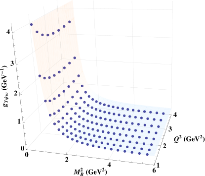
Figure 4: The form factor $g_{{}_{\!Y\!\psi\omega}}(Q^{2})$ as a function of the momentum $Q^{2}$ and Borel mass parameter $M_{B}^{2}$.

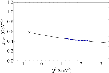
Figure 5: QCDSR results for the form factor $g_{{}_{\!Y\!\psi\omega}}(Q^{2})$, for $\sqrt{s_{0}}=4.40$ GeV (circles). The solid line gives the parametrization of the QCDSR results through Eq. (33). The cross indicates the value of the coupling constant.

In Fig. 4, we show a plot of the form factor $g_{{}_{\!Y\!\psi\omega}}(Q^{2})$ as a function of $M_{B}^{2}$ and $Q^{2}$. Note that, a reliable sum rule must be independent of the choice of Borel mass parameter. As one can see, we obtain a good stability in Borel mass parameter at $M_{B}^{2}\geq 1.8\nobreak\,\mbox{GeV}^{2}$. Here we work at the interval a $1.8~{}\nobreak\,\mbox{GeV}^{2}\leq M_{B}^{2}\leq 4.0~{}\nobreak\,\mbox{GeV}^{2}$. The form factor dependence in $Q^{2}$ can be evaluated by taking the average of the $M_{B}^{2}$ values inside this stability region. The results are shown in Fig. 5.

As mentioned above, the sum rule is not reliable at very large and very small values of $Q^{2}$. Here we find that the results are reliable for $1.2\leq Q^{2}\leq 2.4\nobreak\,\mbox{GeV}^{2}$.

Once we have determined the form factor behavior, we can now extract the coupling constant by using the momentum value at the omega meson pole, $Q^{2}=-M_{\omega}^{2}$. For this purpose, we have to extrapolate the form factor to the region of $Q^{2}$ where the QCDSR is not valid. This extrapolation can be done by parametrizing the QCDSR results shown in Fig. 5 for $g_{{}_{\!Y\!\psi\omega}}(Q^{2})$ using a monopolar function:

$$g_{{}_{\!Y\!\psi\omega}}(Q^{2})=\frac{g_{1}}{g_{2}+Q^{2}},$$ (33)

and the results for the fitting parameters are:

$$g_{1}=(4.0~{}\pm~{}1.0)~{}\mbox{GeV};$$

$$g_{2}=(7.4~{}\pm~{}0.2)~{}\mbox{GeV}^{2}.$$ (34)

The theoretical errors are evaluated considering errors on the following parameters: $\sqrt{s_{0}}=4.40\pm 0.10$ GeV, $\theta=76.0^{\circ}\pm 5.0^{\circ}$, and also the error on the meson coupling parameter $\lambda_{Y}$, given by Eq. (20). We notice that the results do not depend much on the parameters $\sqrt{s_{0}}$ and $\theta$, while the theoretical errors are mainly affected by the meson coupling $\lambda_{Y}$.

In order to see how well the parametrization works, the solid line in Fig. 5 represents the Eq. (33) with values given by Eq. (34). The coupling constant, $g_{{}_{\!Y\!\psi\omega}}$ , is given by using the momentum value $Q^{2}=-M^{2}_{\omega}$ in Eq. (33). Then, we get:

$$g_{{}_{\!Y\!\psi\omega}}=g_{{}_{\!Y\!\psi\omega}}(-M^{2}_{\omega})=(0.58~{}\pm~{}0.14)~{}~{}\mbox{GeV}^{-1}.$$ (35)

The decay width for this process $Y(3940)\rightarrow J/\psi\>\omega$ is given by

$$\Gamma_{{Y(3940)\to J/\psi\>\omega}}=\frac{g^{2}_{{}_{\!Y\!\psi\omega}}}{3}{p(M_{Y},M_{\omega},M_{\psi})\over 8\pi M_{Y}^{2}}\hskip 28.45274pt$$

$$\times\left(M_{\psi}^{2}M_{\omega}^{2}+{1\over 2}(M_{Y}^{2}-M^{2}_{\psi}-M_{\omega}^{2})^{2}\right),$$ (36)

where

$$p(a,b,c)\equiv{\sqrt{a^{4}+b^{4}+c^{4}-2a^{2}b^{2}-2a^{2}c^{2}-2b^{2}c^{2}}\over 2a}.$$ (37)

Therefore, we obtain the decay width inserting the value obtained for the coupling constant (35) in (36):

$$\Gamma_{Y(3940)\to J/\psi\>\omega}=(1.7~{}\pm~{}0.6)~{}\nobreak\,\mbox{MeV}.$$ (38)

This result is consistent with the experimental width of the state and the lower limit for the process $Y\to J/\psi\>\omega$ belleY3940 ; babarY3940 ; godfrey ; godfrey2 . It is also of the same order as other available theoretical evaluations oset ; gutsche .

V Summary and Conclusions

In summary, we have used the QCDSR approach to study the two-point and three-point functions of the $Y(3940)$ state, by considering it as a mixed charmonium-molecule state. We have evaluated the mass working with the two-point function at leading order in $\alpha_{s}$ and we consider the contributions from the condensates up to dimension-8. We obtained a mass which is in a very good agreement with the experimental value for the $Y(3940)$ state, and we found a mixing angle around $\theta=(76.0\pm 5.0)^{0}$.

To evaluate the width of the decay channel $Y(3940)\to J/\psi\>\omega$, we work with the three-point function also at leading order in $\alpha_{s}$ and we consider the contributions from the condensates up to dimension-7. The obtained value of the width is $\Gamma_{Y\to J/\psi\>\omega}=(1.7\pm 0.6)$ MeV, which is smaller than the total experimental width belleY3940 ; babarY3940 , but is consistent with the lower limit for this channel $\Gamma>1$ MeV oset ; gutsche . Thus, according to the available experimental data, we can conclude that a mixing between the $\chi_{c0}$ charmonium and the $D^{\ast}\!\bar{D}^{\ast}$ molecule, could be a good candidate to explain the $Y(3940)$ state.

Acknowledgment

This work has been supported by FAPESP and CNPq.

Appendix A Spectral Densities for the Two-point Correlation Function

Next, we list the spectral densities for the mixed scalar $(\chi_{c0})\!-\!(D^{\ast}\!\bar{D}^{\ast})$ state described by the current in Eq. (1). We consider the OPE contributions up to dimension-8 condensates and keep terms at leading order in $\alpha_{s}$. In order to retain the heavy quark mass finite, we use the momentum-space expression for the heavy quark propagator. We calculate the light quark part of the correlation function in the coordinate-space and use the Schwinger parametrization to evaluate the heavy quark part of the correlator. For the $d^{4}x$ integration in Eq. (5), we use again the Schwinger parametrization, after a Wick rotation. Finally, the result of these integrals are given in terms of logarithmic functions through which we extract the spectral densities. The same technique can be used for evaluating the condensate contributions.

For the $\chi_{c0}$ meson contribution, the spectral densities are written below rry

$$\rho^{pert}_{{}_{\chi_{c0}}}(s) = -\frac{3m_{c}^{2}}{8\pi^{2}}~{}v\left(4-\frac{1}{x}\right)~{}~{},$$

$$\rho^{\langle G^{2}\rangle}_{{}_{\chi_{c0}}}(s) = \frac{\langle g_{s}^{2}G^{2}\rangle}{2^{4}\pi^{2}}\int\limits^{1}_{0}\!d\alpha\>\delta\!\left[s-\frac{m_{c}^{2}}{\alpha(1-\alpha)}\right]$$

$$\times~{}\bigg{(}1-\frac{m_{c}^{2}/M_{B}^{2}}{\alpha(1-\alpha)^{2}}\bigg{)}~{},$$

$$\rho^{\langle G^{3}\rangle}_{{}_{\chi_{c0}}}(s) = \frac{m_{c}^{2}\>\langle g_{s}^{3}G^{3}\rangle}{3\cdot 2^{6}\pi^{2}\>M_{B}^{4}}\int\limits^{1}_{0}\!d\alpha\>\delta\!\left[s-\frac{m_{c}^{2}}{\alpha(1-\alpha)}\right]$$

$$\times~{}\bigg{(}\frac{72-83\alpha+14\alpha^{2}}{\alpha(1-\alpha)^{3}}\bigg{)}~{}~{}.$$

For the $D^{\ast}\bar{D}^{\ast}~{}(0^{++})$ molecular state albuquerque

$$\rho^{pert}_{{}_{D^{\ast}\!D^{\ast}}}(s) = \frac{m_{c}^{8}}{5\cdot 2^{12}\pi^{6}}\bigg{[}v\!\left(480+\frac{1460}{x}-\frac{274}{x^{2}}-\frac{38}{x^{3}}+\frac{1}{x^{4}}\right)$$

$$~{}+120\mathcal{L}_{v}\left(8x-1-6\mbox{\>Log}(x)-\frac{8}{x}+\frac{2}{x^{2}}\right)-1440\mathcal{L}_{+}\bigg{]}~{},$$

$$\rho^{\langle\bar{q}q\rangle}_{{}_{D^{\ast}\!D^{\ast}}}(s) = \frac{m_{c}^{5}\langle\bar{q}q\rangle}{64\pi^{4}}\bigg{[}v\!\left(\!6\!-\!\frac{5}{x}\!-\!\frac{1}{x^{2}}\!\right)\!+\!6\mathcal{L}_{v}\!\left(\!2x\!-\!2\!+\!\frac{1}{x}\!\right)\!\bigg{]}~{},$$

$$\rho^{\langle G^{2}\rangle}_{{}_{D^{\ast}\!D^{\ast}}}(s) = \frac{m_{c}^{4}\langle g_{s}^{2}G^{2}\rangle}{3\cdot 2^{10}\pi^{6}}\bigg{[}v\!\left(\!6\!-\!\frac{5}{x}\!-\!\frac{1}{x^{2}}\!\right)\!+\!6\mathcal{L}_{v}\!\left(\!2x\!-\!2\!+\!\frac{1}{x}\!\right)\!\bigg{]},$$

$$\rho^{\langle\bar{q}Gq\rangle}_{{}_{D^{\ast}\!D^{\ast}}}(s) = \frac{3m_{c}^{3}\langle\bar{q}Gq\rangle}{128\pi^{4}}\left(\frac{v}{x}-2\mathcal{L}_{v}\right)~{},$$

$$\rho^{\langle\bar{q}q\rangle^{2}}_{{}_{D^{\ast}\!D^{\ast}}}(s) = \frac{m_{c}^{2}\>\rho\langle\bar{q}q\rangle^{2}}{4\pi^{2}}~{}v~{},$$

$$\rho^{\langle G^{3}\rangle}_{{}_{D^{\ast}\!D^{\ast}}}(s) = \frac{m_{c}^{2}\langle g_{s}^{3}G^{3}\rangle}{3\cdot 2^{12}\pi^{6}}\!\bigg{[}v\!\left(\!6\!-\!\frac{25}{x}\!+\!\frac{1}{x^{2}}\!\right)\!\!+\!6\mathcal{L}_{v}\!\left(\!2x\!+\!2\!+\!\frac{1}{x}\!\right)\!\!\bigg{]},$$

$$\rho^{\langle 8\rangle}_{{}_{D^{\ast}\!D^{\ast}}}(s)\!\! = -\frac{m_{c}^{2}\langle\bar{q}q\rangle\langle\bar{q}Gq\rangle}{8\pi^{2}}\int\limits_{0}^{1}\!d\alpha~{}\delta\!\left[s-\frac{m_{c}^{2}}{\alpha(1-\alpha)}\right]$$

$$\times~{}\left(1+\frac{m_{c}^{2}/M_{B}^{2}}{\alpha(1-\alpha)}\right)~{}~{}.$$

Finally, for the mixed term, we have

$$\rho^{\langle\bar{q}q\rangle}_{mix}(s) = \frac{m_{c}^{2}\langle\bar{q}q\rangle}{4\pi^{2}}~{}v\left(4-\frac{1}{x}\right)~{},$$

$$\rho^{\langle\bar{q}Gq\rangle}_{mix}(s) = 0~{}~{}.$$

In all these expressions we have used the following definitions:

$$x = m_{c}^{2}/s~{}~{},$$ (39)

$$v = \sqrt{1-4x}~{}~{},$$ (40)

$${\cal L}_{v} = \mbox{Log}\left(\frac{1+v}{1-v}\right)~{}~{},$$ (41)

$${\cal L}_{+} = \mbox{Li}_{2}\left(\frac{1+v}{2}\right)-\mbox{Li}_{2}\left(\frac{1-v}{2}\right)~{}~{}.$$ (42)

References

• [1] S. Uehara et al. [Belle Collaboration], Phys. Rev. Lett.  104, 092001 (2010) [arXiv:0912.4451 [hep-ex]].
• [2] K. Abe et al. [Belle Collaboration], Phys. Rev. Lett.  94, 182002 (2005) [hep-ex/0408126].
• [3] B. Aubert et al. [BaBar Collaboration], Phys. Rev. Lett.  101, 082001 (2008).
• [4] S. Uehara et al. [Belle Collaboration], Phys. Rev. Lett.  96, 082003 (2006) [hep-ex/0512035].
• [5] B. Aubert et al. [BaBar Collaboration], Phys. Rev. D 81, 092003 (2010) [arXiv:1002.0281 [hep-ex]].
• [6] J. P. Lees et al. [BaBar Collaboration], Phys. Rev. D 86, 072002 (2012) [arXiv:1207.2651 [hep-ex]].
• [7] S. Godfrey and S. L. Olsen, Ann. Rev. Nucl. Part. Sci.  58, 51 (2008) [arXiv:0801.3867 [hep-ph]].
• [8] E. Eichten, S. Godfrey, H. Mahlke and J. L. Rosner, Rev. Mod. Phys.  80 (2008) 1161 [hep-ph/0701208].
• [9] X. Liu and S. -L. Zhu, Phys. Rev. D 80, 017502 (2009) [Erratum-ibid. D 85, 019902 (2012)] [arXiv:0903.2529 [hep-ph]].
• [10] T. Branz, T. Gutsche and V. E. Lyubovitskij, Phys. Rev. D 80, 054019 (2009) [arXiv:0903.5424 [hep-ph]].
• [11] T. Branz, R. Molina and E. Oset, Phys. Rev. D 83, 114015 (2011) [arXiv:1010.0587 [hep-ph]].
• [12] R. M. Albuquerque, M. E. Bracco and M. Nielsen, Phys. Lett. B 678, 186 (2009) [arXiv:0903.5540 [hep-ph]].
• [13] M.A. Shifman, A.I. and Vainshtein and V.I. Zakharov, Nucl. Phys. B 147, 385 (1979).
• [14] L.J. Reinders, H. Rubinstein and S. Yazaki, Phys. Rept. 127, 1 (1985).
• [15] For a review and references to original works, see e.g., S. Narison, QCD as a theory of hadrons, Cambridge Monogr. Part. Phys. Nucl. Phys. Cosmol. 17, 1 (2002) [hep-h/0205006]; QCD spectral sum rules , World Sci. Lect. Notes Phys. 26, 1 (1989); Acta Phys. Pol. B26, 687 (1995); Riv. Nuov. Cim. 10N2, 1 (1987); Phys. Rept. 84, 263 (1982).
• [16] J. Sugiyama, T. Nakamura, N. Ishii, T. Nishikawa and M. Oka, Phys. Rev. D 76, 114010 (2007) [arXiv:0707.2533 [hep-ph]].
• [17] R. D’E. Matheus, F. S. Navarra, M. Nielsen and C. M. Zanetti, Phys. Rev. D 80, 056002 (2009) [arXiv:0907.2683 [hep-ph]].
• [18] M. Nielsen and C. M. Zanetti, Phys. Rev. D 82, 116002 (2010) [arXiv:1006.0467 [hep-ph]].
• [19] C. M. Zanetti, M. Nielsen and R. D. Matheus, Phys. Lett. B 702, 359 (2011) [arXiv:1105.1343 [hep-ph]].
• [20] J. M. Dias, R. M. Albuquerque, M. Nielsen and C. M. Zanetti, Phys. Rev. D 86, 116012 (2012) [arXiv:1209.6592 [hep-ph]].
• [21] B.L. Ioffe, Nucl. Phys. B 188, 317 (1981); ibid., Nucl. Phys. B 191, 591(E) (1981).
• [22] B.L. Ioffe and A.V. Smilga, Nucl. Phys. B232, 109 (1984).
• [23] F.S. Navarra, M. Nielsen, Phys. Lett. B 639, 272 (2006); arXiv:hep-ph/0605038.
• [24] M. Nielsen, Phys. Lett. B 634, 35 (2006); arXiv:hep-ph/0510277.