Multiple State Representation Scheme for Organic Bulk Heterojunction Solar Cells: A Novel Analysis Perspective

Abstract

The physics of organic bulk heterojunction solar cells is studied within a six state model, which is used to analyze the factors that affect current-voltage characteristics, power-voltage properties and efficiency, and their dependence on nonradiative losses, reorganization of the nuclear environment, and environmental polarization. Both environmental reorganization and polarity is explicitly taken into account by incorporating Marcus heterogeneous and homogeneous electron transfer rates. The environmental polarity is found to have a non-negligible influence both on the stationary current and on the overall solar cell performance. For our organic bulk heterojunction solar cell operating under steady-state open circuit condition, we also find that the open circuit voltage logarithmically decreases with increasing nonradiative electron-hole recombination processes.

Considerable progress has been achieved in improving the device efficiency of bulk heterojunction (BHJ) organic solar cells, with a recently set record of $10.7\%$. [1, 2] Much of this success came about by searching for promising electron-donor polymers characterized by low optical gap, using fullerene based electron-acceptor derivatives and optimizing the interpenetrated frozen-in microstructures. Such phase-separated blend morphologies are distinguished by a large interface area between the donor and the acceptor phases, which is a prerequisite to tailor most efficient organic photovoltaic solar cells (OPVs). While material design is one successful strategy to improve the OPV setup, another is to focus on the device physics by developing approaches that take into account physical and chemical features of BHJ organic solar cells in order to improve their dynamical operation. In the last two years there appeared several reviews [3, 4, 5, 6, 7] and perspective articles [8, 9] about both material designs and device physics giving an excellent account of the state-of-the-art for organic photovoltaics.

In the context of solar energy conversion, device physics aims to identify routes for improved cell performance by studying models that account for both the material properties and the underlying microscopic principles of the energy conversion processes, i. e. structural and energetics system parameters, in order to identify critical factors that affect the overall OPV performance. Thus, the generated free carriers in a photovoltaic device, which can be harvested at the electrodes, are limited by the complex interplay between charge generation, diffusion, and recombination processes. In BHJ organic solar cells the generation of free charge carriers requires that photoinduced excitons (bounded electron-hole pairs) on the donor material must diffuse to and dissociate at the donor-acceptor (D-A) interface before their recombination takes place. This exciton dissociation at the D-A interface starts with the formation of a charge transfer (CT) state (a geminate pair), where the hole and the electron remain at close proximity on their respective donor and acceptor sites. [7] This CT state can either recombine nonradiatively (geminate recombination), or undergo charge separation leading to mobile electron and hole carriers. [7, 10] However, because of both the low carrier mobility and the interpenetrated nature of typical BHJ blends, there is a non-negligible probability that dissociated free carriers recombine again at the large D-A interface (nongeminate recombination) before being collected at the electrodes. [7, 11] These nonradiative recombinations can be a major loss mechanism that strongly reduces the power conversion efficiency in BHJ solar cells, [12, 13, 14, 15, 16] and are mainly influenced by the energy difference between the highest occupied molecular level $\varepsilon_{\rm D1}$ of D (called HOMO of D) and the lowest unoccupied level $\varepsilon_{\rm A2}$ of A (called LUMO of A). Since it was experimentally found for several donor-acceptor material combinations [17, 18, 5, 19] that the open circuit voltage $U_{\rm oc}$ is proportional to this effective energy gap, the nonradiative recombination losses can be traced back to a drop of $U_{\rm oc}$.

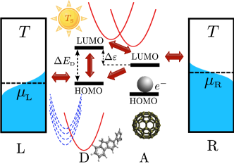
Figure 1: Schematic representation of energetics in BHJ solar cells. The system consists of a donor and acceptor, each characterized by their HOMO and LUMO levels. The metal-molecule coupling is manifested by heterogeneous electron transfer (ET) rates, while transitions between the two molecules are controlled by homogeneous ET rates, both obtained from the Marcus ET theory.

Understanding the relationship between system properties that affect exciton dissociation at the D-A interface and consequently $U_{\rm oc}$ is subject of active research [20, 19, 9]. To study how nonradiative losses at the D-A interface influence the overall device performance, we invoke the minimal model used in our previous publication [21], a solar cell with coupled donor and acceptor molecules, each described as a two-level (HOMO, LUMO) system, in contact with two electrodes, $\rm L$ and $\rm R$ (see Fig. 1). The electrodes are represented by free-electron reservoirs at chemical potentials $\mu_{K}$ ($K=L,R$) that are set to $\varepsilon_{\rm\scriptscriptstyle F}=\varepsilon_{\rm\scriptscriptstyle D1}+\Delta E_{\rm\scriptscriptstyle D}/2$ in the zero-bias junction. In the model studied here a symmetric bias is applied with $\mu_{K}=\varepsilon_{\rm\scriptscriptstyle F}\pm|e|U/2$, where $U$ is the bias voltage. Here, we use the notation $\Delta E_{\rm\scriptscriptstyle K}=\varepsilon_{\rm\scriptscriptstyle K2}-\varepsilon_{\rm\scriptscriptstyle K1}$ ($K=\rm D,\,A$) for the energy differences that represent the donor and acceptor band gaps, and refer to $\Delta\varepsilon=\varepsilon_{\rm\scriptscriptstyle D2}-\varepsilon_{\rm\scriptscriptstyle A2}$ as the interface or donor-acceptor LUMO-LUMO gap. It is important to note that these energies are determined by the detailed electronic structure of the system. Roughly, $\Delta\varepsilon$ is determined by the single electron energies augmented by the exciton binding energy - the sum $E_{\rm\scriptscriptstyle C}=V_{\rm\scriptscriptstyle C}+V_{\rm\scriptscriptstyle C}^{\prime}$, where $V_{\rm\scriptscriptstyle C}>0$ is the Coulombic repulsion between two electrons on the acceptor and $V_{\rm\scriptscriptstyle C}^{\prime}>0$ is the Coulombic energy cost to move an electron away from the donor. Furthermore, interaction with the nuclear environment, expressed under equilibrium conditions by the nuclear reorganization energy, affects this energy gap as described below. The different system states are described by occupation numbers $n_{\rm\scriptscriptstyle K_{j}}=0,1$, where $K=D,A$ and $j=1,2$. In order to use a minimal model that contains essential physical pictures we limit the number of system states as follows. First, an imposed restriction $n_{\rm\scriptscriptstyle D1}n_{\rm\scriptscriptstyle D2}=0$ ensures that the donor cannot be double occupied. In addition we set $n_{\rm\scriptscriptstyle A1}=1$, so that the acceptor can only receive an additional electron. The resulting minimal model then consists of six states with respect to the occupations $(n_{\rm\scriptscriptstyle D1},\,n_{\rm\scriptscriptstyle D2},\,n_{\rm\scriptscriptstyle A1},\,n_{\rm\scriptscriptstyle A2})$, that we denote by the integers $j=0,\,...,\,5$, [see Fig. 2(a)]. Within this six-state representation, the probability to find the system in state $j$ is denoted by $P_{j}$.

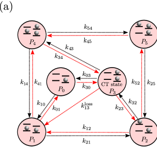
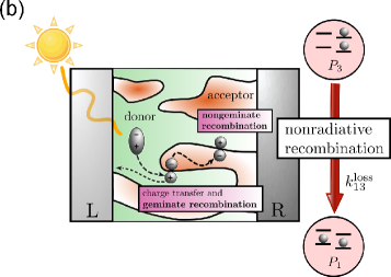
Figure 2: (a) Network representation of the underlying master equation associated with the six accessible microstates. The graph is composed of six vertices (shown as circles). The interconnected vertices represent the probabilities $P_{j}$ to find the system in a microstate $j$ ($j=0,...,5$) and the edges connecting some pairs of vertices stand for transitions between the states. The edges are drawn as arrows that indicate transitions with rate $k_{j^{\prime}\,j}=k_{j^{\prime}\leftarrow j}$ from a state (vertex) $j$ to $j^{\prime}$. (b) The recombination process. With a certain probability, electrons transferred into the LUMO of the acceptor in state $P_{3}$ can recombine with the hole left on the donor (geminate recombination) or migrate in the acceptor phase and recombine with the donor at another interfacial position (nongeminate recombination). Both processes eventually lead, following nonradiative relaxation, to state $P_{1}$, reducing the number of carriers collected at the electrodes.

This minimal model of a BHJ solar cell accounts for the important interfacial electronic processes, including excitation, exciton dissociation, carrier recombination and electron transfer (ET) processes. In order to focus on these interfacial processes we disregard in this model exciton diffusion in the donor and charge carrier diffusion in the acceptor phase, but obviously a more complete model should take these important processes of the cell operation into account [22]. In particular, the ET processes are affected by environmental polarization relaxation. This is taken here into account using the nonadiabatic Marcus theory, which is based on the assumption that in each electronic state the nuclear motion reaches thermal equilibrium quickly (fast relative to rates of change of electronic states). The relevant rates are associated with the following processes:

(a) The electron transfer between the left electrode $\mathrm{L}$ to the HOMO of the donor is determined by heterogeneous Marcus rates [23] [see also Fig. 2(a)],

$$k_{10}=k_{43}=\frac{\nu_{\rm\scriptscriptstyle L}}{\sqrt{4\pi\lambda_{\rm\scriptscriptstyle D}k_{\rm B}T}}\int dE\,f(E)e^{-\frac{\scriptstyle(E+\mu_{\rm\scriptscriptstyle L}-\varepsilon_{{\rm\scriptscriptstyle D1}}-\lambda_{\rm\scriptscriptstyle D})^{2}}{\scriptstyle 4\lambda_{\rm\scriptscriptstyle D}k_{\rm B}T}}\,,$$ (1)

where $\nu_{\rm\scriptscriptstyle L}$ is the inverse of a characteristic time scale involved in this process, $\lambda_{\rm\scriptscriptstyle D}$ is the reorganization energy associated with the response of the nuclear environment to electronic population on the donor (also called inner-sphere reorganization energy [24]), and $k_{\rm B}T$ is the thermal energy. Here, $f(x)=1/[\exp(x)+1]$ with $x=E/k_{\rm B}T$ and $T$ is the cell temperature. A similar expression, with $\mu_{\rm\scriptscriptstyle L}$, $\nu_{\rm\scriptscriptstyle L}$, and $\lambda_{\rm\scriptscriptstyle D}$ replaced by $\mu_{\rm\scriptscriptstyle R}$, $\nu_{\rm\scriptscriptstyle R}$, and $\lambda_{\rm\scriptscriptstyle A}$ applies for electron transfer rates $k_{03}=k_{14}=k_{25}$ from the LUMO of the acceptor to the right electrode $R$. The corresponding reverse rates, e.g.,

$$k_{01}=k_{34}=\frac{\nu_{\rm\scriptscriptstyle L}}{\sqrt{4\pi\lambda_{\rm\scriptscriptstyle D}k_{\rm B}T}}\int dE\,\tilde{f}(E)e^{-\frac{\scriptstyle(E+\mu_{\rm\scriptscriptstyle L}-\varepsilon_{{\rm\scriptscriptstyle D1}}+\lambda_{\rm\scriptscriptstyle D})^{2}}{\scriptstyle 4\lambda_{\rm\scriptscriptstyle D}k_{\rm B}T}}\,,$$ (2)

where $\tilde{f}(E)=1-f(E)$, satisfy detailed balance.

(b) Light absorption and molecular excitation take place at the donor with photon absorption leading to an exciton (electron in an excited state D2) with rate $k_{21}=k_{54}=\nu_{\rm\scriptscriptstyle{S}}n_{\rm\scriptscriptstyle{S}}(x_{\rm\scriptscriptstyle{S}})$, where $n_{\rm{\scriptscriptstyle S}}=1/\left[\exp(x_{\rm{\scriptscriptstyle S}})-1\right]$ with $x_{\rm{\scriptscriptstyle S}}=\Delta E_{\rm{\scriptscriptstyle D}}/k_{\rm B}T_{\rm{\scriptscriptstyle S}}$ [25]. $T_{\rm{\scriptscriptstyle S}}$ is the sun temperature representing the incident radiation and $\nu_{\rm\scriptscriptstyle{S}}$ determines the characteristic time scale for this process. Excited states can radiatively decay with rates $k_{12}=k_{45}=\nu_{\rm\scriptscriptstyle{S}}(1+n_{\rm\scriptscriptstyle{S}}(x_{\rm\scriptscriptstyle{S}}))$.

(c) The dissociation of an exciton at the D-A interface leads to a CT state $P_{3}$ with a homogeneous rate given by a Marcus-type expression

$$k_{32} =\frac{\nu_{\rm\scriptscriptstyle DA}}{\sqrt{4\pi{\lambda}_{{\rm\scriptscriptstyle DA}}k_{\rm B}T}}e^{-\frac{\scriptstyle({\varepsilon}_{\rm\scriptscriptstyle DA}-{\lambda}_{{\rm\scriptscriptstyle DA}})^{2}}{\scriptstyle 4{\lambda}_{{\rm\scriptscriptstyle DA}}k_{\rm B}T}}\,,$$

$$k_{23} =\frac{\nu_{\rm\scriptscriptstyle DA}}{\sqrt{4\pi{\lambda}_{{\rm\scriptscriptstyle DA}}k_{\rm B}T}}e^{-\frac{\scriptstyle({\varepsilon}_{\rm\scriptscriptstyle DA}+{\lambda}_{{\rm\scriptscriptstyle DA}})^{2}}{\scriptstyle 4{\lambda}_{{\rm\scriptscriptstyle DA}}k_{\rm B}T}}\,,$$ (3)

where $\varepsilon_{\rm\scriptscriptstyle DA}=\varepsilon_{\rm\scriptscriptstyle D2}-(\varepsilon_{\rm\scriptscriptstyle A2}+E_{\rm\scriptscriptstyle C})+E_{\rm\scriptscriptstyle P}$. $E_{\rm\scriptscriptstyle P}$ is the term associated with the energy change of charge states, where the electron is on the donor or on the acceptor. If the environmental polarization motions (or modes) that respond to charging are different for the donor and the acceptor species, the reorganization energy for the ET transfer at the D-A interface is $\lambda_{\rm\scriptscriptstyle DA}=\lambda_{\rm\scriptscriptstyle D}+\lambda_{\rm\scriptscriptstyle A}$ [23]. Since the physical origin of $E_{\rm\scriptscriptstyle P}$ and $\lambda_{\rm\scriptscriptstyle DA}$ is the same, they are related to each other. The details of this relationship depend on how reorganization occurs on transition between the initial and final state of the electron transfer process. In our case, environmental polarization stabilizes the charge separated state relative to the parent excitonic configuration. More generally [26] if some reorganization exists already in the absence of environmental polarity it changes according to $\lambda_{\rm\scriptscriptstyle DA}\rightarrow\lambda_{\rm\scriptscriptstyle DA}+E_{\rm\scriptscriptstyle P}$. In either case the forward rate is not affected by increasing environmental polarity while the backward process is inhibited.

(d) In the six-state model nonradiative (geminate and nongeminate) recombination of electron and holes at the D-A interface will together be represented by an effective recombination rate $k_{13}^{\rm\scriptscriptstyle loss}$ [see Fig. 2(b)]. However, future work should take into account the fact that the geminate and nongeminate rates depend differently on the densities of electrons and holes, as for example in a rate equation description. In fact, a rate equation description should imply that the geminate rate is proportional to the number of geminate electron-hole pairs, while the nongeminate contribution depends on the product of electron and hole densities at the interface.

The system dynamics is modeled by a master equation approach accounting for the time evolution of the probabilities $P_{j}(t)$ ($j=0,...,5$) fulfilling normalization $\sum_{j}P_{j}(t)=1$ at all times. [27, 28, 29, 30, 31, 32] An elegant network representation [33] can be used to depict the transitions between the six possible states shown in Fig. 2(a). Starting from this, the currents can be written in terms of state probabilities as follows

$$J_{\rm\scriptscriptstyle L}(t) =k_{10}(P_{0}+P_{3})-k_{01}(P_{1}+P_{4})$$ (4)

$$J_{\rm\scriptscriptstyle R}(t) =k_{03}(P_{3}+P_{4}+P_{5})-k_{30}(P_{0}+P_{1}+P_{2})$$ (5)

$$J_{\rm\scriptscriptstyle S}(t) =k_{21}(P_{1}+P_{4})-k_{12}(P_{2}+P_{5})$$ (6)

$$J_{\rm\scriptscriptstyle DA}(t) =k_{32}P_{2}-k_{23}P_{3}$$ (7)

$$J_{\rm\scriptscriptstyle loss}(t)\mathbf{} =k_{13}^{\rm\scriptscriptstyle loss}P_{3}\,.$$ (8)

$J_{\rm\scriptscriptstyle L}$ ($J_{\rm\scriptscriptstyle R}$) is the current entering (leaving) the molecular system from (to) the electrodes, $J_{\rm\scriptscriptstyle S}$ is the light induced transition current between the HOMO and the LUMO in the donor phase, and $J_{\rm\scriptscriptstyle DA}$ is the current between the donor and acceptor species. $J_{\rm\scriptscriptstyle loss}$ is the loss current which includes both geminate and nongeminate recombination processes at the D-A interface. The steady-state solution of the underlying master equation is given by Kirchhoff’s current law [34] for each state $j=0,..,5$, i. e. the net influx must equal the net outflux at each vertex. For example, for $j=0$, the node condition is $0=k_{01}P_{1}(t)+k_{03}P_{3}(t)-\left(k_{10}+k_{30}\right)P_{0}(t)$ [see Fig. 2(a)]. Applying this procedure to each state leads to a closed set of coupled linear equations. In what follows we specify the steady-state current $J_{\rm\scriptscriptstyle L}=J_{\rm\scriptscriptstyle R}=J_{\rm\scriptscriptstyle S}-J_{\rm\scriptscriptstyle loss}=J_{\rm\scriptscriptstyle DA}-J_{\rm\scriptscriptstyle loss}\equiv J$.

In order to demonstrate the nature of the kinetics we consider the following set of parameters:  $\mu_{\rm\scriptscriptstyle L}=\varepsilon_{\rm\scriptscriptstyle D1}+(\Delta E_{\rm\scriptscriptstyle D}-|e|U)/2$, $\mu_{\rm\scriptscriptstyle R}=\mu_{\rm\scriptscriptstyle L}+|e|U$, $\varepsilon_{\rm\scriptscriptstyle D1}=-0.1\,\rm eV$,$\varepsilon_{\rm\scriptscriptstyle D2}=1.4\,\rm eV$, $\varepsilon_{\rm\scriptscriptstyle A2}=0.8\,\rm eV$, $V_{\rm\scriptscriptstyle C}=0.25\,\rm eV$, and $V_{\rm\scriptscriptstyle C}^{\prime}=0.15\,\rm eV$. Thus, $\Delta E_{\rm\scriptscriptstyle D}=\varepsilon_{\rm\scriptscriptstyle D2}-\varepsilon_{\rm\scriptscriptstyle D1}=1.5\,\rm eV$ [35] and $E_{\rm\scriptscriptstyle C}=0.4\,\rm eV$ [36, 8]. For the temperatures we choose $T=300\rm K$ and $T_{s}=6000\rm K$. The kinetic rates are set to $\nu_{\rm\scriptscriptstyle L}=\nu_{\rm\scriptscriptstyle R}=\nu_{\rm\scriptscriptstyle S}=0.01\nu_{\rm\scriptscriptstyle DA}$ and $\nu_{\rm\scriptscriptstyle DA}=10^{12}$s^-1. For simplicity we assume that the reorganization energies $\lambda_{\rm\scriptscriptstyle D}$ and $\lambda_{\rm\scriptscriptstyle A}$ in the donor and acceptor phase are both $0.1\,\rm eV$.

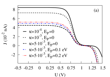
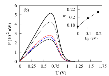
Figure 3: (a) Steady-state current and (b) power as functions of bias voltage for three different rate ratios $\kappa=k_{13}^{\rm\scriptscriptstyle loss}/k_{32}$ and polarity energies $E_{\rm\scriptscriptstyle P}$. In (b) the assignment of lines is given in the legend (a). The inset in (b) shows the thermodynamic efficiency at maximum power [21] as function of $E_{\rm\scriptscriptstyle P}$ for $\kappa=5\cdot 10^{-3}$.

The behaviors of the current- and power-voltage characteristics as functions of both the nonradiative losses and environmental polarity are shown in Fig. 3. Figure 3(a) shows the current-voltage characteristics for different $E_{\rm\scriptscriptstyle P}$ values and several rate ratios $\kappa=k_{13}^{\rm\scriptscriptstyle loss}/k_{32}$, which measure the magnitude of the recombination losses compared to the fast ET transfer at the D-A interface. Obviously the steady-state current decreases with increasing losses. In particular, the plateau in the $J(U)$ curve drops down with larger $k_{13}^{\rm\scriptscriptstyle loss}$. For a certain applied voltage value $U_{\rm oc}$ the current is zero and becomes negative for $U>U_{\rm oc}$. To demonstrate the influence of the environmental polarity we choose $\kappa=5\cdot 10^{-3}$ and two different polarity energies $E_{\rm\scriptscriptstyle P}=0.1$ eV and $0.2$ eV. Compared to the curve corresponding to $E_{\rm\scriptscriptstyle P}=0$ and $\kappa=5\cdot 10^{-3}$ we find a significant increase in the current. Figure 3(b) compares the performance $P(U)=UJ(U)$ of the BHJ solar cell for various loss currents and environmental polarity energies. Clearly, the curves in Fig. 3(b) exhibit a maximum in the region where the current in Fig. 3(a) decreases sharply. We also observe that the performance of the solar cell strongly depends on both environmental polarization relaxation and nonradiative losses. In particular, the inset in Fig. 3(b) shows the dependence of the thermodynamic efficiency $\eta$ on $E_{\rm\scriptscriptstyle P}$ for $\kappa=5\cdot 10^{-3}$. Because the maximum power output is shifted to larger $U$ by increasing $E_{\rm P}$, the solar cell becomes more efficient by increasing the environmental polarization.

Next, we analyze the steady-state performance of the BHJ solar cell operating under open circuit condition [$J(U_{\rm oc})=0$].

Figure 4: Open circuit voltage as function of rate ratio $\kappa$ for vanishing $E_{\rm\scriptscriptstyle P}$ (filled circles) and for $E_{\rm\scriptscriptstyle P}=0.2$ eV (open circles). The inset shows $U_{\rm oc}$ as function of the effective band gap $|\varepsilon_{\rm\scriptscriptstyle D1}-\varepsilon_{\rm\scriptscriptstyle A2}|$ of the D-A blend for $\kappa=10^{-3}$.

Figure 4 shows $U_{\rm oc}$ calculated for the chosen parameter set as function of $\kappa$. Increasing nonradiative loss rates leads to a decrease in the open circuit voltage, in agreement with earlier findings [20, 4] As a result, we find that $U_{\rm oc}$ is proportional to $\ln(\kappa)$ [see filled circles for $E_{\rm\scriptscriptstyle P}=0$ in Fig. 4]. It is also interesting to see how these results change upon increasing environmental polarity, in particular because it inhibits recombination but at the same time makes a larger LUMO-LUMO gap. The open circuit voltage increases by considering environmental polarity [see Fig. 4]. In the inset of Fig. 4 we study the influence of the effective band gap $|\varepsilon_{\rm\scriptscriptstyle D1}-\varepsilon_{\rm\scriptscriptstyle A2}|$ on $U_{\rm oc}$. We observe that our BHJ solar cell model well accounts for the present common understanding that $U_{\rm oc}$ is linearly proportional to the effective bandgap. For example, let us consider a donor HOMO level of $\varepsilon_{\rm\scriptscriptstyle D1}=-0.1$  eV and a rate ratio $\kappa=k_{13}^{\rm\scriptscriptstyle loss}/k_{32}=10^{-3}$, where we vary $k_{32}$ and consequently also the acceptor LUMO level $\varepsilon_{\rm\scriptscriptstyle A2}$. We then have $U_{\rm oc}=|\varepsilon_{\rm\scriptscriptstyle D1}-\varepsilon_{\rm\scriptscriptstyle A2}|/|e|-a(\kappa)$. The value of the parameter $a$ depends on $\kappa$ [37]. For $\kappa=10^{-3}$, the fit yields $a(\kappa=10^{-3})=0.17$, which corresponds to the dashed line in the inset of Fig. 4.

In conclusion, we developed a model using a six-state representation for a D-A blend which accounts for essential aspects of the device physics of BHJ solar cells. In particular, we incorporated more realistically the molecule-reservoir coupling in terms of heterogeneous Marcus rates and the ET process at the D-A interface by homogeneous Marcus rates. In addition we have demonstrated how nonradiative (geminate and nongeminate) processes can be captured within a six-state representation. We also discussed the influence of environmental polarity on the charge separation process. The environmental polarity turned out to have a decisive influence on both the stationary current and the overall solar cell performance. Focusing on a BHJ cell operating under steady-state open circuit condition, we observed a less pronounced influence of the environmental polarity on $U_{\rm oc}$ and found $U_{\rm oc}$ proportional to $\ln(\kappa)$ by varying the rate ratio $\kappa$. Regarding future generalizations that include hot electrons [8, 38, 39] and tail states [18], the present model provides a framework for analyzing the open circuit voltage behavior.

1 Acknowledgement

We thank Carsten Deibel for illuminating discussions on geminate and nongeminate recombination processes, and an anonymous referee for useful comments. M.E. gratefully acknowledges funding by a Minerva Short-Term Research Grant. The research of A.N. is supported by the Israel Science Foundation, the Israel-US Binational Science Foundation (grant No. 2011509), and the European Science Council (FP7/ERC grant No. 226628).

References

- [1] \NameService R. F. \REVIEWScience 3322011293.
- [2] In April 2012, Heliatek (www.heliatek.com) reported that an organic tandem solar cell achieved a power conversion efficiency of on a cm2 substrate. Organic solar cells with power conversion efficiencies are considered to be competitively viable with inorganic solar cells.
- [3] \NameDennler G., Scharber M. C. Brabec C. J. \REVIEWAdv. Mater. 2120091323.
- [4] \NameDeibel C. Dyakonov V. \REVIEWRep. Prog. Phys. 732010096401.
- [5] \NameNicholson P. G. Castro F. A. \REVIEWNanotechnology 212010492001.
- [6] \NameThompson B. C., Khlyabich P. P., Burkhart B., Aviles A. E., Rudenko A., Shultz G. V., Ng C. F. Mangubat L. B. \REVIEWGreen 1201129.
- [7] \NameNelson J. \REVIEWMaterials Today 142011462.
- [8] \NamePensack R. D. Asbury J. B. \REVIEWJ. Phys. Chem. Lett. 120102255.
- [9] \NameCredgington D. Durrant J. R. \REVIEWJ. Phys. Chem. Lett. 320121465.
- [10] \NameAndersson L. M., Müller C., Badada B. H., Zhang F., Würfel U. Inganas O. \REVIEWJ. Appl. Phys. 1102011024509.
- [11] \NameGluecker M., Foertig A., Dyakonov V. Deibel C. \REVIEWPhys. Status Solidi RRL 62012337.
- [12] \NameNelson J., Kirkpatrick J. Ravirajan P. \REVIEWPhys. Rev. B 692004035337.
- [13] \NameKirchartz T., Taretto K. Rau U. \REVIEWJ. Phys. Chem. C 113200917958.
- [14] \NameKirchartz T., Pieters B. E., Taretto K. Rau U. \REVIEWPhys. Rev. B 802009035334.
- [15] \NameGiebink N. C., Wiederrecht G. P., Wasieleswski M. R. Forrest S. R. \REVIEWPhys. Rev. B 832011195326.
- [16] \NameGruber M., Wagner J., Klein K., Hörmann U., Opitz A., Stutzmann M. Brütting W. \REVIEWAdv. Energy Mater. 220121100.
- [17] \NameScharber M. C., Mühlbacher D., Koppe M., Denk P., Waldauf C., Heeger A. J. Brabec C. J. \REVIEWAdv. Mater. 182006789.
- [18] \NameNayak P. K., Bisquert J. Cahen D. \REVIEWAdv. Mater. 2320112870.
- [19] \NameRauh D., Wagenpfahl A., Deibel C. Dyakonov V. \REVIEWAppl. Phys. Lett. 982011133301.
- [20] \NameMaurano A., Hamilton R., Shuttle C. G., Ballantyne A. M., Nelson J., O Regan B., Zhang W., McCulloch I., Azimi H., Morana M., Brabec C. J. Durrant J. R. \REVIEWAdv. Mater. 2220104987.
- [21] \NameEinax M., Dierl M. Nitzan A. \REVIEWJ. Phys. Chem. C 115201121396.
- [22] \NameDierl M., Einax M. Nitzan A. in preparation.
- [23] \NameNitzan A. \BookChemical Dynamics in Condensed Phases: Relaxation, Transfer, and Reactions in Condensed Molecular Systems 1st Edition (Oxford University Press, Oxford) 2006.
- [24] \NameVaissier V., Barnes P., Kirkpatrick J. Nelson J. \REVIEWPhys. Chem. Chem. Phys. 1520134804.
- [25] \NameRutten B., Esposito M. Cleuren B. \REVIEWPhys. Rev. B 802009235122.
- [26] On transition from state a to state a , if the two corresponding parabolic nuclear potential surfaces are and , introducing an additional environmental polarity response such that implies so that and .
- [27] \NameEinax M., Solomon G. C., Dieterich W. Nitzan A. \REVIEWJ. Chem. Phys. 1332010054102.
- [28] \NameEinax M., Körner M., Maass P. Nitzan A. \REVIEWPhys. Chem. Chem. Phys. 122010645.
- [29] \NameDierl M., Maass P. Einax M. \REVIEWEurophys. Lett. 93201150003.
- [30] \NameDierl M., Maass P. Einax M. \REVIEWPhys. Rev. Lett. 1082012060603.
- [31] \NameDierl M., Einax M. Maass P. \REVIEWPhys. Rev. E 872013062126.
- [32] \NameSylvester-Hvid K. O., Rettrup S. Ratner M. A. \REVIEWJ. Chem. B, 10820044296.
- [33] \NameSchnakenberg J. \REVIEWRev. Mod. Phys. 481976571.
- [34] \NameKirchhoff G. \REVIEWAnn. Phys. (Berlin) 1481847497.
- [35] \NameSoci C., Hwang I.-W., Moses D., Zhu Z., Waller D., Gaudiana R., Brabec C. J. Heeger A. J. \REVIEWAdv. Funct. Mater. 172007632.
- [36] \NameGregg B. A. Hanna M. C. \REVIEWJ. Appl. Phys. 9320033605.
- [37] \NameKoster L. J. A., Shaheen S. E. Hummelen J. C. \REVIEWAdv. Energy Mater. 220121246.
- [38] \NameGrancini G., Maiuri M., Fazzi D., Petrozza A., Egelhaaf H.-J., Brida D., Cerullo G. Lanzani G. \REVIEWNature Mater. 12201329.
- [39] \NameJailaubekov A. E., Willard A. P., Tritsch J. R., Chan W.-L., Sai N., Gearba R., Kaake L. G., Williams K. J., Leung K., Rossky P. J. Zhu X.-Y. \REVIEWNature Mater. 12201366.