A review of beam tomography research at Daresbury Laboratory

Abstract

This is a review on beam tomography research at Daresbury. The research has focussed on development of normalised phase space techniques. It starts with the idea of sampling tomographic projections at equal phase advances and shows that this would give the optimal reconstruction results. This idea has influenced the design, construction and operation of the tomography sections at the Photo Injector Test Facility at Zeuthen (PITZ) and at the Accelerator and Laser in Combined Experiments (ALICE) at Daresbury. The theoretical justification of this idea is later developed through simulations and analysis of the measurements results at ALICE. The mathematical formalism is constructed around the normalised phase space and the idea of equal phase advances become the basis of this. This formalism is applied to a variety of experimental and simulated situations and shown to be useful in improving resolution, increasing reliability and providing diagnostic information. In this review, we also present the simplifying concepts, formalisms and simulation tools that we have developed.

I Introduction

Phase space tomography Stratakis ; McKee is a measurement technique that is used in accelerators to characterise the phase space of a particle beam. It has been used in a number of accelerators, including PITZ Asova2 , UMER Stratakis2 , SNS, PSI Reggiani , CERN CERN , BNL Yakimenko , FLASH Honkavaara and TRIUMF Rao2 . The beam distribution measured in coordinate space can be mapped mathematically to a phase space, and the rotation angle in the phase space can be varied by changing the strengths of optical elements along the beamline. This mapping to rigid rotation makes it possible to reconstruct the phase space distribution using standard tomographic techniques.

In a simple implementation, the optical element could just be a drift space. Suppose that we wish to determine the transverse, horizontal phase space at a particular location in a beamline. Suppose that there is a scintillating screen at a second location further along the beamline. The horizontal phase space at the screen is related to that at the first location. Assuming linear mapping, the relation can be represented by a matrix. This matrix produces a geometrical transformation on the phase space, usually a combination of shearing and stretching. The tomographic method involves projecting the screen image on the horizontal axis. The geometric connection means that this can be related to the projection of the phase space at the first location in a rotated direction. This angle can be varied by changing the length of the drift space. By measuring the projections for a range of drift distances, the projections for a range of angles at the first location can be obtained. The phase space distribution can be reconstructed from these projections using techniques like Filtered Back Projection (FBP) or Maximum Entropy Technique (MENT). In practice, the setup will involve a combination of drift spaces and other elements, such as quadrupoles or solenoids. Measurements on longitudinal phase space also require RF cavities. In this review we focus on transverse phase space.

Phase space tomography has been implemented in different ways in a number of accelerators. At ALICE Ibison , it follows closely the basic theory described above. It uses a quadrupole to change the rotation angle by changing the quadrupole strength. The quadrupole strength is varied using a computer, and screen images are captured automatically and then processed using FBP. However, the range of angles accessible by a single quadrupole is limited to a smaller range than the full 180^∘. At PITZ Asova2 , the rotation angle is varied using a combination of drift spaces and quadrupoles. In practice it may not be easy to build a setup to move a screen mechanically along a beampipe in order to vary the drift distance. The PITZ tomography section consists of four screens to measure the beam distribution in coordinate space at different locations along the beampipe. The quadrupole strengths are not normally varied during a measurement. This means that only four projections are measured. This small number of projection angles makes it better to use MENT for reconstruction. At ALICE, PSI and SNS Reggiani , the tomography diagnostic sections have also been designed for MENT with between three and five screens. At TRIUMF Rao2 , a wire scanner with a quadrupole is used instead of screens. There are wires in three fixed angles. These measure the projections in three directions in the transverse coordinate space. MENT is used for reconstruction. At UMER Stratakis2 , the strengths of a few quadrupoles are adjusted to obtain the full 180^∘ range of angles. The reconstruction is carried out using FBP. The reconstruction algorithm is modified to include space charge effects.

Phase space tomography research at ALICE over the past three years has focussed on two main areas: development of the normalised phase space method, and more recently development of 4D reconstruction. Development of the normalised phase space method has been primarily motivated by the idea of using equal phase advances in phase space tomography Asova . The phase advance here refers to betatron phase advance Lee . There at four screens separated by FODO cells. This setup is designed to give 45^∘ phase advance in between adjacent screens in transverse phase space in both horizontal and vertical directions. Together, the four screens give four projections at equal phase advances over 180^∘. This design has been adopted for the construction of the PITZ tomography section and used in tomographic measurements since then Asova2 . The same idea has been used in the design and construction of the ALICE tomography section Muratori ; Muratori2 . There are three screens with FODO cells in between adjacent screens. Phase advance between adjacent screens is adjusted to be 60^∘. This gives three projections with equal phase advances in between. However, at ALICE we have not had the chance to carry out such a measurement. In the beam time available, we have mainly used a quadrupole scan in which the quadrupole strength is varied rapidly using a computer and images captured at a single screen.

At PITZ where only four projections are available, MENT is used for reconstructing the phase space. The use of such a small amount of measured data to reconstruct the whole phase space means that the magnitude of error is uncertain. Simulations on hypothetical distributions at PITZ have demonstrated that using equal phase advances give the smallest error in emittances of reconstructed distributions Asova1 . However, at the time of the construction of first PITZ and then ALICE, there has been no theoretical justification as to why equal phase advances should produce optimal reconstructions. This has been a question because there is no obvious connection between phase advance and the method of phase space tomography. The only angle that exists in phase space tomography is the projection angle and this is not equal to phase advance. The explanation comes later when we show that the phase advance is in fact equal to the projection angle in normalised phase space Hock . A Gaussian distribution in normalised phase space would appear roughly circular. Having equal phase advances means sampling projections at equal angles in this phase space. This would be the natural sampling interval, particularly if variation of distribution with angle is small. Conversely, a distribution in real phase space tends to be long and narrow because of long drift spaces in beamlines. Such a distribution varies strongly with angle. Using equal angle intervals would either sample too little in the sharply varying directions or require too many projections over the full 180^∘ range.

This realisation has not only provided a theoretical justification for the idea and use of equal phase advances. It also opens up new areas of applications. So far, we have shown that normalised phase space can improve resolution for FBP Hock , reduce distortion for MENT Hock1 , and detect linear errors in reconstructions Ibison . In section II, we summarise the main steps leading to the formulae for tomography in general. In section III, we provide a simple derivation of phase space tomography formalism that we have developed. In section IV, we provide a simple derivaton of MENT. In section V, we explain how we use FBP in practice. In section VI, we review the idea of equal phase advances and how it has influenced the design of tomography sections at PITZ and ALICE. In section VII, we explain our normalised phase space method and show how phase advance is connected to projection angles. In section VIII, we summarise our measurement procedure at ALICE and the reconstruction results. In section IX, we explain an idea to observe space charge at the ALICE tomography section using normalised phase space. In section X, we review the use of normalised phase space to improve the reliability of MENT reconstructions. In section XI, we conclude with a summary and a discussion on what we plan to do next.

II Tomography

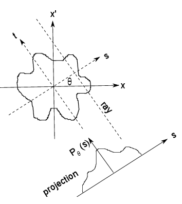
Figure 1:

We review here the basic theory of tomography. The goal is essentially to derive a formula to calculate a 2D distribution function $f(x,x^{\prime})$ from its projections. The following steps are summarised from Kak .

We first define the projection. Consider the axes $(s,t)$ rotated by angle $\theta$ in Fig. 1. The coordinates are related to $(x,x^{\prime})$ by

$$s =x\cos\theta+x^{\prime}\sin\theta$$

$$t =-x\sin\theta+x^{\prime}\cos\theta$$ (1)

The projection of $f(x,x^{\prime})$ along $s$ axis is given by

$$P_{\theta}(s)=\int_{-\infty}^{\infty}f(x(s,t),x^{\prime}(s,t))dt$$ (2)

This is an integral along a line of constant $s$. This line is called a ray. It is perpendicular to the $s$ axis, which is the direction of the projection.

The Fourier transform of the projection is

$$S_{\theta}(w)=\int_{-\infty}^{\infty}P_{\theta}(s)e^{-i2\pi ws}ds$$ (3)

Substituting the definition of projection

$$S_{\theta}(w)=\int_{-\infty}^{\infty}\left[\int_{-\infty}^{\infty}f(x,x^{\prime})dt\right]e^{-i2\pi ws}ds$$ (4)

and transforming to $(x,x^{\prime})$ coordinates

$$S_{\theta}(w)=\int_{-\infty}^{\infty}\int_{-\infty}^{\infty}f(x,x^{\prime})e^{-i2\pi w(x\cos\theta+x^{\prime}\sin\theta)}dxdx^{\prime}$$ (5)

In terms of the following coordinates

$$u =w\cos\theta$$

$$v =w\sin\theta$$ (6)

we see that $S_{\theta}(w)$ is the same as the 2D Fourier transform

$$F(u,v)=\int_{-\infty}^{\infty}\int_{-\infty}^{\infty}f(x,x^{\prime})e^{-i2\pi(xu+x^{\prime}v)}dxdx^{\prime}$$ (7)

So

$$S_{\theta}(w)=F(w,\theta)=F(w\cos\theta,w\sin\theta)$$ (8)

where $(w,\theta)$ are the polar coordinates in the 2D spatial frequency domain.

Inverting the transform gives

$$f(x,x^{\prime})=\int_{-\infty}^{\infty}\int_{-\infty}^{\infty}F(u,v)e^{i2\pi(ux+vx^{\prime})}dudv$$ (9)

Transforming to polar coordinates:

$$f(x,x^{\prime})=\int_{0}^{2\pi}\int_{0}^{\infty}F(w,\theta)e^{i2\pi w(x\cos\theta+x^{\prime}\sin\theta)}wdwd\theta$$ (10)

Next split this into two parts:

$$f(x,x^{\prime})=\int_{0}^{\pi}\int_{0}^{\infty}F(w,\theta)e^{i2\pi w(x\cos\theta+x^{\prime}\sin\theta)}wdwd\theta$$

$$+\int_{0}^{\pi}\int_{0}^{\infty}F(w,\theta+\pi)e^{i2\pi w[x\cos(\theta+\pi)+x^{\prime}\sin(\theta+\pi)]}wdwd\theta$$ (11)

Then use this property of Fourier transform:

$$F(w,\theta+\pi)=F(-w,\theta)$$ (12)

and rewrite the transform as:

$$f(x,x^{\prime})=\int_{0}^{\pi}\left[\int_{-\infty}^{\infty}F(w,\theta)|w|e^{i2\pi ws}dw\right]d\theta$$ (13)

where $F(w,\theta)$ is the Fourier transform of the projection $S_{\theta}(w)$:

$$f(x,x^{\prime})=\int_{0}^{\pi}\left[\int_{-\infty}^{\infty}S_{\theta}(w)|w|e^{i2\pi ws}dw\right]d\theta$$ (14)

This provides the relation between projections and function $f(x,x^{\prime})$.

The Filtered Back Projection technique for computing $f(x,x^{\prime})$ from the projections is obtained by defining

$$Q_{\theta}(s)=\int_{-\infty}^{\infty}S_{\theta}(w)|w|e^{i2\pi ws}dw$$ (15)

Multiplying a Fourier transform $S_{\theta}(w)$ by a function $|w|$ of frequency and then inverting the transform is often called filtering. Since $S_{\theta}(w)$ is the Fourier transform of the projection, $Q_{\theta}(s)$ is called the filtered projection.

From Eq. (14)

$$f(x,x^{\prime})=\int_{0}^{\pi}Q_{\theta}(s)d\theta$$ (16)

This is like spreading $Q_{\theta}(s)$ back over the $(x,x^{\prime})$ space and then summing up for all angles. For this reason, $Q_{\theta}(s)$ is called the back projection.

In principle, the two equations above can be discretised and used to reconstruct $f(x,x^{\prime})$ numerically from the projections $P_{\theta}(s)$. This reconstruction technique is called Filtered Back Projection.

III Phase Space Tomography

A standard derivation of the equations used in beam tomography is given in McKee . Rather than just summarising the results, we reproduce here an alternative derivation which gives insight into the geometric nature of the method.

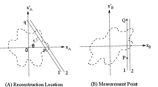
Figure 2: The $x$ intercept $a$ at A is mapped to point P at B, and $y$ intercept $b$ is mapped to point Q. Projection variable $s$ at A corresponds to projection variable $x_{B}$ at B.

We need to derive the relation between a projection at B in the $x_{B}$ direction and the corresponding projection at A. Specifically, we want to find (i) a formula for the direction $\theta$ of the projection at A; (ii) a formula to relate projection variables $s$ and $x_{B}$; and (iii) a formula to relate a projection at B to a projection at A. We assume that the mapping is given:

$$\begin{pmatrix}x_{B}\\ x_{B}^{\prime}\end{pmatrix}=\begin{pmatrix}M_{11}&M_{12}\\ M_{21}&M_{22}\end{pmatrix}\begin{pmatrix}x_{A}\\ x_{A}^{\prime}\end{pmatrix}$$ (17)

The effect of this mapping is a geometrical transformation. For a drift space, it is a shear in the $x$ direction, as illustrated in Fig. 2. For a thin quadrupole, it is a shear in the $x^{\prime}$ direction. For other elements, it could be some combination of shear, stretch and rotation.

Consider a ray line 1 at B in Fig. 2 and the corresponding ray line 1 at A. Line 1 at A is mapped to line 1 at B by the mapping in Eq. (17). The intercepts $p$ and $q$ at A are mapped to points P and Q at B. The coordinates of P are $(pM_{11},pM_{21})$. The coordinates of Q are $(qM_{12},qM_{22})$. Since P and Q lie on the same vertical line, they have the same $x_{B}$ coordinate:

$$x_{B}=pM_{11}=qM_{12}.$$ (18)

From triangle 0pq in Fig. 2, angle $\theta$ is equal to angle 0qp. So the tangent of the angle $\theta$ is $p/q$. From Eq. (18), we obtain:

$$\tan\theta=\frac{p}{q}=\frac{M_{12}}{M_{11}}.$$ (19)

This gives the formula for the direction $\theta$ of the projection at A.

From Eq. (18), the ratio $x_{B}/s$ is equal to $pM_{11}/s$. From triangle 0pq in Fig. 2, $p/s$ is equal to $\sec\theta$. Using the identity $1+\tan^{2}\theta=\sec^{2}\theta$, Eq. (19) gives

$$\frac{x_{B}}{s} =\frac{aM_{11}}{s}$$

$$=M_{11}\sec\theta$$

$$=M_{11}\sqrt{1+\tan^{2}\theta}$$

$$=M_{11}\sqrt{1+\frac{M_{12}^{2}}{M_{11}^{2}}}$$

$$=\sqrt{M_{11}^{2}+M_{12}^{2}}$$ (20)

This ratio is the scaling factor $a$ relating projection variables $s$ and $x_{B}$.

Compare the distance interval between lines 1 and 2 at B, and the corresponding interval at A. The interval at A is clearly scaled down by the above scaling factor $a$. Since the number of particles within this interval must be the same at A and at B, the projection $p_{A}$ at A must be scaled up from the projection $p_{B}$ at B by $a$. This observation gives the formula to transform a projection at B to a projection at A:

$$p_{A}(s)=ap_{B}(as),$$ (21)

where $a$ is $x_{B}/s$.

This completes the derivation. The full set of equations needed to transform projections from measurement point to reconstruction location are:

$$\tan\theta=\frac{M_{12}}{M_{11}}.$$ (22)

$$a=\sqrt{M_{11}^{2}+M_{12}^{2}}.$$ (23)

$$s=\frac{x_{B}}{a}$$ (24)

$$p_{A}=ap_{B},$$ (25)

After this transformation, each projection at A corresponds to a simple rotation by angle $\theta$.

IV Maximum Entropy Technique

Our implementation of MENT follows closely the formalism described in Mottershead . We provide here a simpler derivation that allows us to replace most of the mathematical steps leading to the MENT equation with a pictorial explanation.

The initial steps in the MENT theory would be familiar to students of physics who have studied the derivation of Boltzmann distribution. In a quantum system of particles, each particle can only occupy discrete energy levels. There are different arrangements of particles that can give the same number at each level. The Boltzmann distribution is the most likely distribution. This is obtained by finding the distribution that has the greatest number of arrangements. Each arrangement must obey the constraints that the total number of particles and the total energy are both fixed.

In MENT, we divide a region of phase space into a grid of tiny squares as shown in Fig. 3. Each square corresponds to an energy level. A phase space distribution tells us the number of particles in each square. MENT aims to find the most likely distribution. This is obtained by finding the one with the largest number of possible arrangements. The constraints are that the resulting distribution must give projections that agree with the measured ones at each angle.

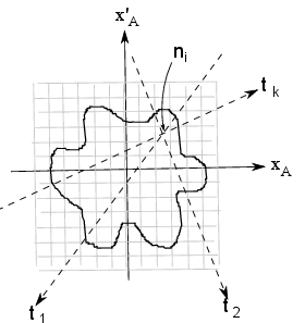
Figure 3: The phase space is divided into a grid of tiny squares. Each line labelled $t_{k}$ that goes through square $i$ is a ray that is parallel to the $t$ axis of projection angle $k$.

We first review the mathematical steps leading to the Boltzmann distribution Glazer , and then show how this can be generalised directly to MENT. Consider a system of $N$ distinguishable particles. Each particle can occupy the energy levels $\epsilon_{i}$, and there are $n_{i}$ particles at each level. The constraints are that the number of particles

$$N=n_{1}+n_{2}+...$$ (26)

and the total energy

$$U=n_{1}\epsilon_{1}+n_{2}\epsilon_{2}+...$$ (27)

are fixed. A distribution is given by the set of numbers $(n_{1},n_{2},...)$. The number of possible arrangements for this distribution is:

$$W=\frac{N!}{n_{1}!n_{2}!...}$$ (28)

We want to find the distribution for which $W$ is maximum. This would be easier if we maximise $\ln W$ instead because Stirling’s approximation makes the factorials simpler:

$$\ln W\approx(N\ln N-N)-(n_{1}\ln n_{1}-n_{1})-(n_{2}\ln n_{2}-n_{2})-...$$ (29)

In physics, entropy is given by $k_{B}\ln W$ where $k_{B}$ is Boltzmann’s constant. Hence the name Maximum Entropy Technique. We then apply the method of Lagrange multipliers Glazer . First we make the Lagrange function

$$L=\ln W+\lambda_{0}\sum n_{i}+\lambda_{1}\sum n_{i}\epsilon_{i}$$ (30)

where the second and third terms on the right come from the two constraints above, and $\lambda_{0}$ and $\lambda_{1}$ are called Lagrange multipliers. If we now maximise $L$ with respect to $(n_{1},n_{2},...)$, we would get the most likely distribution under the given constraints. First we differentiate and set the derivative to zero:

$$\frac{\partial L}{\partial n_{i}}=-\ln n_{i}+\lambda_{0}+\lambda_{1}\epsilon_{i}=0$$ (31)

Then we solve for $n_{i}$:

$$n_{i}=e^{\lambda_{0}}e^{\lambda_{1}\epsilon_{i}}$$ (32)

When $\lambda_{1}$ is replaced with $-1/k_{B}T$ using thermodynamic reasoning, we get the familiar Boltzmann distribution.

To apply this to MENT, we replace energy levels with the tiny squares in phase space. The formula for the number of arrangements $W$ is the same. The constraint on the number of particles $N$ is also the same. The constraint on total energy is now replaced by the constraints that the projections for the distribution must agree with the the measured ones:

$$p_{k}(s_{k})=\sum_{t_{k}}n_{i}$$ (33)

The left side of this equation is the projection value for the angle $k$ and coordinate $s_{k}$. The subscript $t_{k}$ of the summation on the right side means that only those tiny squares on the ray at angle $k$ and coordinate $s_{k}$ are included in the sum. The ray indicated by $t_{k}$ is illustrated in Fig. 3. The length of a ray in one square is different from its length in another square. The size of each square is assumed to be very small so that the sum over $t_{k}$ approaches an integral.

The Lagrange function is then given by

$$L=\ln W+\lambda_{0}\sum n_{i}+\sum_{k}\sum_{s_{k}}\lambda_{k}(s_{k})\sum_{t_{k}}n_{i}$$ (34)

$s_{k}$ is assumed to be discrete with very small steps so that the sum over $s_{k}$ approaches an integral. In Mottershead, the integral signs would be used for both the sumes over $s_{k}$ and $t_{k}$. We retain the summation signs to simplify the next step.

To maximise $L$, we differentiate with respect to $n_{i}$:

$$\frac{\partial L}{\partial n_{i}}=0=-\ln n_{i}+\lambda_{0}+\sum_{k}\lambda_{k}(s_{k})$$ (35)

To understand the sum on the right, observe that all $n$ variables should vanish except $n_{i}$ because the differentiation is with respect to $n_{i}$. Recall that $n_{i}$ is the population of particles at a particular tiny square. The multipliers $\lambda_{k}(s_{k})$ that remain must correspond to those rays that pass through the centre of this particular square, as illustrated in Fig. 3. The number of rays is just the number of projections. $s_{k}$ would be the coordinate of the square’s centre for each projection. With this understanding, we now rearrange to get

$$n_{i}=e^{\lambda_{0}}\prod_{k=1}^{K}e^{\lambda_{k}(s_{k})}$$ (36)

where $K$ is the number of measured projections. This can be rewritten as

$$f(x,x^{\prime})=\prod_{k}h_{k}(s_{k})$$ (37)

where we have defined

$$h_{k}(s_{k})=e^{\lambda_{k}(s_{k})+\lambda_{0}/K}$$ (38)

We have equated the number density function $f(x,x^{\prime})$ to the population $n_{i}$. This is correct up to a constant factor.

The key result is that the number density $f(x_{A},x_{A}^{\prime})$ of particles in phase space at the reconstruction location A can be expressed as a product of certain functions. Each of these functions has only one variable, and this variable is the distance along each projection direction $s$ (see Fig. 1). This relation can be written as

$$f(x_{A},x_{A}^{\prime})=\prod_{k=1}^{K}h_{k}(s_{k}(x_{A},x_{A}^{\prime})),$$ (39)

Recall the constraint that $f(x_{A},x_{A}^{\prime})$ must give the correct projection that has been measured for each projection. The $k^{th}$ projection is related to $f(x_{A},x_{A}^{\prime})$ by

$$p_{k}(s_{k})=\int f(x_{A},x_{A}^{\prime})dt_{k}$$ (40)

where $t_{k}$ is the axis perpendicular to the $s_{k}$ axis, and the integral is over the range of $t_{k}$ where $f(x_{A},x_{A}^{\prime})$ is nonzero. The coordinates $(x_{A},x_{A}^{\prime})$ are determined for each value of $s_{k}$ given on the left of the equation and each value of $t_{k}$ defined during the integration. This means that if $f(x_{A},x_{A}^{\prime})$ is known, then when we integrate it along the $t_{k}$ direction for a given $s_{k}$ value, the answer must be equal to the value of the projection at $s_{k}$.

Equations (39) and (40) fully define the mathematical problem and the distribution $f(x_{A},x_{A}^{\prime})$ can in principle be solved.

Using Eqs. (39) and (40), we can now solve for the distribution $f(x_{A},x_{A}^{\prime})$. By substituting Eq. (39) into Eq. (40), we get

$$p_{k}(s_{k})=h_{k}(s_{k})\int dt_{k}\prod_{k^{\prime}\not=k}^{K}h_{k^{\prime}}(s_{k^{\prime}}(x_{A},x_{A}^{\prime}))$$ (41)

where $h_{k}(s_{k})$ is factored out. This is possible because $s_{k}$ and $t_{k}$ are the coordinates of the $k^{th}$ projection $p_{k}(s_{k})$, so $s_{k}$ does not change when $t_{k}$ is varied in the integral. Equation (41) makes it possible to solve for the unknown $h_{k}(s_{k})$ using a technique known as Gauss-Seidel iteration:

1. Rearrange Eq. (41) for iteration:

   $$h_{k}^{i+1}(s_{k})=\frac{p_{k}(s_{k})}{\int dt_{k}\prod_{{k^{\prime}}\neq k}h_{k^{\prime}}^{i}[s_{k^{\prime}}(x_{A},x_{A}^{\prime})]}$$ (42)

   where $h_{k}^{i}(s_{k})$ is the result for $h_{k}(s_{k})$ after $i$ iterations.

2. Use initial values of $h_{k}^{0}(s_{k})=1$.

3. Use Eqs. (39) and (40) to calculate the projections for from the $i^{th}$ iteration:

   $$p_{k}^{i}(s_{k})=\int dt_{k}\prod_{{k^{\prime}}=1}^{K}h_{k^{\prime}}^{i}[s_{k^{\prime}}(x_{A},x_{A}^{\prime})].$$ (43)

4. Calculate the differences between $p_{k}^{i}(s_{k})$ and the measured $p_{k}(s_{k})$ for all $s_{k}$.

5. Repeat the iteration until this difference is small enough for all $s_{k}$. (For the calculations in this paper, we stop when the difference at each pixel $(x_{A},x_{A}^{\prime})$ is less than a tolerance level of 1% of the peak value of $f(x_{A},x_{A}^{\prime})$).

The computed projections may not always converge to the measured projections. We have found that if the projections are too noisy or if they remain non-zero up to the limits of the domain of $s_{n}$, the method fails. For the projections used in this paper, convergence is usually achieved after 3 or 4 iterations.

V FBP in Practice

In this section, we explain the main steps involved in processing measured projections. We also describe simulation tools we have used to validate reconstruction codes.

V.1 Centre of reconstruction

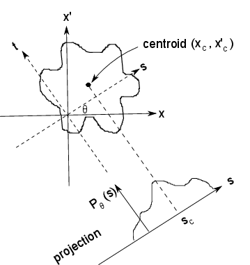
Figure 4: A distribution in which the centroid is not at the origin.

In measured projections, there is a key information that is missing for the reconstruction. It is the origin. In the derivaton of the Filtered Back Projection technique, notice that each projection has an origin. Consider what happens if the origin of one projection is in error. Then during reconstruction, one of the back projections would be shifted. When this is added to other back projections, the result would clearly be erroneous. Unfortunately, in measured projections, we do not know where the origin of each projection is. This is not an issue that is normally discussed in papers on phase space tomography. Here, we describe our solution. We shall prove that if we take the centroid of each projection to be its origin, the resulting reconstruction would be identical to the actual distribution.

Our solution is to use the centroid of each projection as the origin.

To show that this gives the correct reconstruction, consider a hypothetical distribution $f(x,x^{\prime})$ in phase space. Its centroid position is given by:

$$x_{c} =\int\int xf(x,x^{\prime})dxdx^{\prime}$$ (44)

$$x_{c}^{\prime} =\int\int x^{\prime}f(x,x^{\prime})dxdx^{\prime}$$ (45)

Suppose that the centroid is not at the origin. So the centroid of the projection $P_{\theta}(s)$ is also not at its origin $s=0$. Suppose that it is at $s_{c}$. From Fig. 4, this is given by

$$s_{c}=x_{c}\cos\theta+x_{c}^{\prime}\sin\theta$$ (46)

Suppose that we use this as the origin for reconstruction. The centroid can be determined directly from a measured projection using the centroid formula

$$s_{c}=\int sP_{\theta}(s)ds$$ (47)

This would return the same value using any arbitrary point as $s=0$. Taking $s_{c}$ as the origin of a projection, the new projection is

$$P_{\theta}^{\prime}(s)=P_{\theta}(s-s_{c})$$ (48)

If we now put this through the FBP equations, we first obtain the Fourier transform of $P_{\theta}^{\prime}(s)$. From the property of Fourier transform or from Eq. (3):

$$S_{\theta}^{\prime}(w)=e^{-i2\pi ws_{c}}S_{\theta}(w)$$ (49)

From Eq. (8), we can write this as

$$S_{\theta}^{\prime}(w)=F^{\prime}(w,\theta)=e^{-i2\pi ws_{c}}F(w,\theta)$$ (50)

Substituting into Eq. (9) gives

$$f^{\prime}(x,x^{\prime}) =\int_{-\infty}^{\infty}\int_{-\infty}^{\infty}F^{\prime}(u,v)e^{i2\pi(ux+vx^{\prime})}dudv$$ (51)

$$=\int_{-\infty}^{\infty}\int_{-\infty}^{\infty}e^{-i2\pi ws_{c}}F(u,v)e^{i2\pi(ux+vx^{\prime})}dudv$$ (52)

Substituting Eqs. (46) and (6) gives

$$f^{\prime}(x,x^{\prime})=\int_{-\infty}^{\infty}\int_{-\infty}^{\infty}e^{-i2\pi(ux_{c}+vx_{c}^{\prime})}F(u,v)e^{i2\pi(ux+vx^{\prime})}dudv$$ (53)

Finally, comparing with Eq. (9) gives

$$f^{\prime}(x,x^{\prime})=f(x-x_{c},x^{\prime}-x_{c}^{\prime})$$ (54)

This completes the proof that the distribution reconstructed using the projection centroids as origins is identical to the actual distribution $f(x,x^{\prime})$, up to a rigid translation.

V.2 Nonuniform angle intervals

In the usual implementation of FBP, Eq. (16) is discretised as

$$f(x,x^{\prime})=\frac{\pi}{K}\sum_{k=1}^{K}Q_{\theta_{k}}(x\cos\theta_{k}+x^{\prime}\sin\theta_{k})$$ (55)

where Eq. (1) is used to express $s$ in terms of $x$ and $x^{\prime}$. The angle interval given by $\pi/K$ is assumed to be uniform. This is usually valid, for example in X-ray Computer Aided Tomography scan in which rotation angles can be precisely controlled.

In phase space tomography, it is convenient to allow the angle intervals to be different. The main reason is that the angle is varied by changing the strengths of optical elements. This variation need not be linear. In the case of a quadrupole with a drift space for example, the variation can be a combination of steep and gentle. An analytic formula for projection angle in terms of quadrupole current is available. In principal, it should be possible to develop a numerical code to compute precise values of currents required for uniform angles. In practice, we obtain the currents from tabulated values of currents and angles using linear interpolation. To check the accuracy of the currents obtained in this way, the analytic formula is used to compute the corresponding angles. The results show that this procedure is prone to numerical errors. We may find that the actual intervals are not exactly uniform. We can then correct for this by simply using the actual angle intervals in the back projection equation. So Eq. (55) should be written as

$$f(x,x^{\prime})=\sum_{k=1}^{K}Q_{\theta_{k}}(x\cos\theta_{k}+x^{\prime}\sin\theta_{k})\Delta\theta_{k}$$ (56)

where $\Delta\theta_{k}$ is the actual angle interval.

Two other (hopefully) less common situations where this would be useful are when there is a systematic error in the quadrupole current or an error in beam energy at the stage of determining the required currents. Suppose that these errors are discovered after the measurements. Because the projection angle does not vary linearly with current or energy, the resulting reconstruction could be completely wrong. One option would be to redo the experiment. But there is another option. We can recompute the angles using the corrected currents and energy. The new angle intervals can then be used in Eq. (56) and the correct distribution computed.

V.3 Hypothetical Gaussian distribution

Whether it is to verify a reconstruction code written by others or to check a code written by ourselves, it is useful to verify the reconstruction procedure using a hypothetical distribution with known projections. Reconstructing using these projections must obviously return the original distribution. If it does not, then we know there is an error in the code.

In tomography in general, it is common to use a distribution made up of ellipses of different shapes, sizes and brightness. An example is the Shepp Logan phantom which consists of ellipses arranged to look like organs in a cross-section of a human body. There are simple formulae to compute the projections of the combination of ellipses Kak . In phase space tomography, these ellipses with sharp edges do not look realistic. Instead, it is better to use Gaussian distributions. Fortunately, we can also derive analytic formulae for the projections of a Gaussian distribution. We would like to be able to describe the distribution using Twiss parameters and compute the projection for a given transfer matrix. We list here the formulae that we have derived and used for the simulations shown in later sections.

Suppose that we need a Gaussian distribution at reconstruction location A with emittance $\epsilon$, beta function $\beta$ and alpha function $\alpha$. The Gaussian distribution is given by

$$f(x_{A},x_{A}^{\prime})=\exp\left(-\frac{x_{N}^{2}+x_{N}^{\prime 2}}{a_{0}^{2}}\right)$$ (57)

where

$$a_{0}=\sqrt{\epsilon}$$ (58)

and

$$\left(\begin{array}[]{c}x_{N}\\ x^{\prime}_{N}\end{array}\right)=\left(\begin{array}[]{cc}\frac{1}{\sqrt{\beta}}&0\\ \frac{\alpha}{\sqrt{\beta}}&\sqrt{\beta}\end{array}\right)\cdot\left(\begin{array}[]{c}x_{A}\\ x_{A}^{\prime}\end{array}\right).$$ (59)

This is just the transformation to a normalised phase space.

Suppose that it is mapped to the screen at location B where the horizontal projection is measured. Suppose that the mapping is given by matrix $R_{0}$. Then the distribution at B is

$$f(x_{B},x_{B}^{\prime})=\exp\left(-\frac{x_{N}^{2}+x_{N}^{\prime 2}}{a_{0}^{2}}\right)$$ (60)

where

$$\left(\begin{array}[]{c}x_{B}\\ x^{\prime}_{B}\end{array}\right)=R_{0}\left(\begin{array}[]{c}x_{A}\\ x_{A}^{\prime}\end{array}\right).$$ (61)

The projection along $x_{B}$ axis is given by

$$p(x_{B})=\int_{-\infty}^{\infty}f(x_{B},x_{B}^{\prime})dx_{B}^{\prime}$$ (62)

Doing the integration gives

$$p(x_{B})=a_{0}\sqrt{A\pi}\exp\left(-\frac{Ax_{B}^{2}}{a_{0}^{2}}\right)$$ (63)

where

$$A =(a^{2}+c^{2})-Be^{2}$$ (64)

$$e =(ab+cd)/B$$ (65)

$$B =b^{2}+d^{2}$$ (66)

$$\left(\begin{array}[]{cc}a&b\\ c&d\end{array}\right)=N_{1}R_{0}^{-1}$$ (67)

and $N_{1}$ is the matrix in Eq. (59).

VI Equal Phase Advances

As far as we can trace in the literature, the idea of using equal phase advances in phase space tomography may have originated from a simulation study on emittance measurement for the Tesla Test Facility Castro . This empirical study shows that when 4 screens at 45^∘ phase advances in a FODO lattice are used, the emittance computed using images from the 4 screens has the smallest error.

The Tesla Test Facility design described in Castro consists of two diagnostic sections at two different locations. Both are intended for measuring emittance, not phase space tomography. Each section consists of 4 screens. Between each pair of adjacent screens is a FODO cell. The three FODO cells form a short periodic structure. The intention is to measure the beamwidths at the 4 screens. Together with the transfer matrices of the FODO cells, the emittance can then be calculated Castro .

In this study, the strengths of the FODO cells are optimised to reduce the errors of measurement. The following procedure is adopted:

1. The FODO structure is assumed to be infinitely periodic. So the beta functions are determined by the periodicity condtion.

2. The phase advances are then computed. These would be equal between adjacent screens since the structure is periodic.

3. In the actual beamline, the FODO structure is not infinitely periodic. So the actual magnets along the beamline must be adjusted to match the beam to the FODO struture before a measurement.

A simulation is then carried out in Castro to determine the performance. This simulation determines how the error in measured emittance would vary with error in beam size measurement at each screen. A random error is added to the beam sizes and the emittance calculated. This is repeated for 1000 times and the RMS emittance error is determined. This is then repeated for a number of phase advances. The result shows that the RMS emittance error is smallest when phase advance between adjacent screens is 45^∘.

This result has provided the justification for the design of the PITZ tomography section Asova1 . This has a similar design as the diagnostic section in the Tesla Test Facility, with 4 screens and a FODO cell in between each pair of adjacent screens. This FODO structure is also designed to give 45^∘ in between screens. This design was developed by a collaboration between PITZ and Daresbury. It has subsequently influenced the design of the ALICE tomography section.

The ALICE section has 3 screens and a FODO cell in between adjacent screens. This is perhaps the first active use of the idea of equal phase advances for phase space tomography. Whereas the PITZ choice of 45^∘ phase advance is empirically justified by emittance studies, no such study has been carried for ALICE. The choice of 60^∘ phase advance for the ALICE tomography section comes from dividing 180^∘ by 3. The “180^∘” figure comes from the full angular range for tomographic projections. The result in Castro that 45^∘ phase advance is optimal is associated conceptually with tomographic projection angles - 45^∘ is 180^∘ divided by 4, the number of screens. So at ALICE, 180^∘ divided by 3 because there are 3 screens. There is thus a conceptual leap from empirical emittance study to phase space tomography.

Figure 5 shows a schematic diagram of the two FODO cells at the ALICE tomography section and the beta functions computed using MAD8 under the assumption that the FODO cells are periodic Muratori . Figure 5 shows the lattice of ALICE magnets before the tomography section and the beta functions of this lattice that are matched using MADX to the periodic beta functions at the entrance to the tomography section.

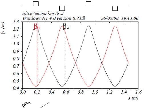
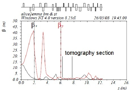
Figure 5: (a) Beta functions at ALICE tomography section, assuming that the FODO lattice is periodic. (b) Beta functions along beamline is matched into entrance of tomography section.

At the time of the construction of ALICE, there has been no further elaboration on this, whether it is emittance study or theoretical analysis. This comes later when we show in Hock that phase advance is equal to projection angle interval in normalised phase space.

VII Normalised Phase Space

In this section, we shall review the steps in Hock to show that phase advance is equal to projection angle interval in normalised phase space.

Recall that phase advance corresponds to rotation angles in the normalised phase space. We assume that there is no coupling between vertical and horizontal motion between reconstruction location and measurement point (e.g. screen). This would be true if we only use quadrupoles and drift spaces. Then the horizontal, transverse normalised phase space at the reconstruction location is defined by the following transformation:

$$\left(\begin{array}[]{c}x_{N}\\ x_{N}^{\prime}\end{array}\right)=\left(\begin{array}[]{cc}\frac{1}{\sqrt{\beta}}&0\\ \frac{\alpha}{\sqrt{\beta}}&\sqrt{\beta}\end{array}\right)\left(\begin{array}[]{c}x_{A}\\ x_{A}^{\prime}\end{array}\right).$$ (68)

$x_{N}$ and $x_{N}^{\prime}$ are the corresponding co-ordinates in the normalised phase space, and $\alpha$ and $\beta$ are Twiss parameters. The Twiss parameters are determined by the second moments of the beam distribution:

$$\langle x^{2}\rangle =\beta\epsilon$$ (69)

$$\langle xx^{\prime}\rangle =-\alpha\epsilon$$ (70)

$$\langle x^{\prime 2}\rangle =\gamma\epsilon$$ (71)

$$\epsilon =\sqrt{\langle x^{2}\rangle\langle x^{\prime 2}\rangle-\langle xx^{\prime}\rangle^{2}}$$ (72)

A similar transformation to Eq. (68) applies to the vertical displacement $y$. Reconstruction in normalised phase space can be done with a simple extension of the method given in section III. A matrix transforms the initial distribution at the reconstruction location to the distribution at the screen. Based on this matrix, the procedure in section III reconstructs the initial distribution.

The initial distribution may be considered the result of the transformation of the distribution in normalised phase space to real phase space. The transformation is given by the inverse of Eq. (68). In order to reconstruct in normalised phase space, we only need to replace the matrix in Eq. (17), by a matrix that transforms the distribution all the way from the normalised phase space to the distribution at the screen. This matrix is simply a product of the matrix in Eq. (17), and the matrix that transforms from normalised to real phase space. The latter matrix may be obtained by inverting Eq. (68) as follows:

$$\left(\begin{array}[]{c}x_{A}\\ x_{A}^{\prime}\end{array}\right)=\left(\begin{array}[]{cc}\sqrt{\beta_{A}}&0\\ -\frac{\alpha_{A}}{\sqrt{\beta_{A}}}&\frac{1}{\sqrt{\beta_{A}}}\end{array}\right)\left(\begin{array}[]{c}x_{N}\\ x_{N}^{\prime}\end{array}\right)$$ (73)

where the subscript A means that the Twiss parameters refer to position A. The matrix on the right hand side is the required matrix. Inserting this into the right hand side of Eq. (17) gives the new transfer matrix $\tilde{M}$ needed for the reconstruction in normalised phase space:

$$\tilde{M}=\left(\begin{array}[]{cc}M_{11}&M_{12}\\ M_{21}&M_{22}\end{array}\right)\left(\begin{array}[]{cc}\sqrt{\beta_{A}}&0\\ -\frac{\alpha_{A}}{\sqrt{\beta_{A}}}&\frac{1}{\sqrt{\beta_{A}}}\end{array}\right)$$ (74)

We now demonstrate that the projection angle $\theta$ in the normalised phase space is equal to the phase advance $\mu$. This can be done using the relation between the transfer matrix and the Twiss parameters at positions A and B:

$$\left(\begin{array}[]{cc}M_{11}&M_{12}\\ M_{21}&M_{22}\end{array}\right)=$$ (77)

$$\left(\begin{array}[]{cc}\sqrt{\frac{\beta_{B}}{\beta_{A}}}(\cos\mu+\alpha_{A}\sin\mu)&\sqrt{\beta_{B}\beta_{A}}\sin\mu\\ \frac{\alpha_{A}-\alpha_{B}}{\sqrt{\beta_{B}\beta_{A}}}\cos\mu-\frac{1+\alpha_{B}\alpha_{A}}{\sqrt{\beta_{B}\beta_{A}}}\sin\mu&\sqrt{\frac{\beta_{A}}{\beta_{B}}}(\cos\mu-\alpha_{B}\sin\mu)\end{array}\right)$$ (80)

where the subscript B means that the Twiss parameters refer to position B. This can also be written as

$$\left(\begin{array}[]{cc}M_{11}&M_{12}\\ M_{21}&M_{22}\end{array}\right)=\left(\begin{array}[]{cc}\sqrt{\beta_{B}}&0\\ -\frac{\alpha_{B}}{\sqrt{\beta_{B}}}&\frac{1}{\sqrt{\beta_{B}}}\end{array}\right) \left(\begin{array}[]{cc}\cos\mu&\sin\mu\\ -\sin\mu&\cos\mu\end{array}\right)$$ (87)

$$\times\left(\begin{array}[]{cc}\frac{1}{\sqrt{\beta_{A}}}&0\\ \frac{\alpha_{A}}{\sqrt{\beta_{A}}}&\sqrt{\beta_{A}}\end{array}\right)$$ (90)

We can understand the right hand side in a simple way: the distribution at A (reconstruction location) is transformed to normalised phase space, propagated to B (screen) by a rigid rotation through angle $\mu$, and transformed back to real phase space. Substituting this into Eq. (74), we find:

$$\tilde{M}=\left(\begin{array}[]{cc}\sqrt{\beta_{B}}&0\\ -\frac{\alpha_{B}}{\sqrt{\beta_{B}}}&\frac{1}{\sqrt{\beta_{B}}}\end{array}\right)\left(\begin{array}[]{cc}\cos\mu&\sin\mu\\ -\sin\mu&\cos\mu\end{array}\right)$$ (91)

We can now apply Eq. (19) to this matrix to find $\theta$. Note that the original transfer matrix $R$ in Eq. (17) has been changed to $\tilde{M}$ defined in Eq. (74). So $M_{11}$ and $M_{12}$ in Eq. (19) must also be replaced by the elements in the first row of Eq. (74). These are equal to those in the first row of Eq. (91), which are $\sqrt{\beta_{B}}\cos\mu$ and $\sqrt{\beta_{B}}\sin\mu$. Substituting these into Eq. (19) for $M_{11}$ and $M_{12}$ respectively, we find:

$$\tan\theta=\tan\mu.$$ (92)

So $\mu$ is indeed the projection angle.

At this stage, we emphasise that the significant result is that if the tomographic reconstruction is performed without a normalising transformation, then the projection angles need to be calculated from the transfer matrices: they are not simply the phase advances. This is significant for tomography at PITZ an ALICE, which are designed with uniform betatron phase advance between successive screens Holder ; Loehl ; Asova , i.e. uniform distribution of projection angles in normalised phase space. The distribution of angles in real phase space will not necessarily be uniform. This would have a direct impact on the reconstruction.

To illustrate this point, consider the corresponding rays in real and normalised phase spaces shown in Fig. 6. (The projection direction is perpendicular to the ray.) Fig. 6 shows a Gaussian distribution in real phase space, with rays that are at uniform angular intervals. In normalised phase space, some of the intervals become smaller, whereas others become larger, as shown in Fig. 6. Fig. 7 illustrates the effect of the opposite transformation – starting with uniform intervals of angles in normalised phase space, shown in Fig. 7. This results in a nonuniform distribution of rays in real phase space, shown in Fig. 7. These observations have direct impact on the reconstruction. The actual effect depends on whether FBP or MENT is used.

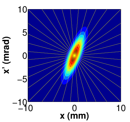
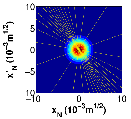
Figure 6: (a) Real phase space with rays at uniform angular intervals. (b) Normalised phase space.

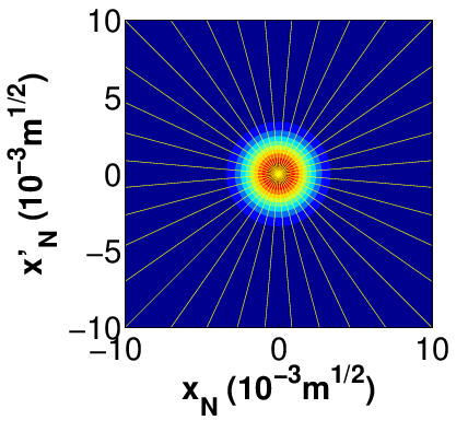
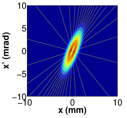
Figure 7: (a) Normalised phase space with rays at uniform angular intervals. (b) Real phase space.

Beam distributions are often more complex than simple Gaussians. We consider a more complex hypothetical case where the distribution is made up of a group of closely spaced Gaussian spots, as shown in Fig. 8. This provides a test of the ability of a reconstruction method to resolve the spots. Note that each spot has a circular distribution in normalised phase space. Assume a hypothetical system of eighteen screens separated only by drift spaces. The projection angle corresponding to each screen can be chosen by adjusting the length of the drift space using Eq. (19). Start with the case of equal angular intervals in real phase space. The projections from the screens are used to reconstruct Fig. 8. The result is shown in Fig. 8. The spots are all reproduced and at the correct positions. However the resolution is less clear.

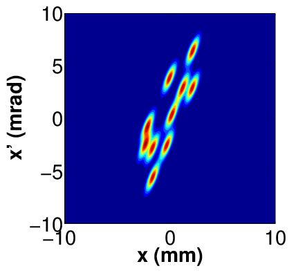
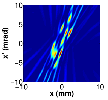
Figure 8: (a) Distribution in real phase space. (b) Reconstruction in real phase space.

We then look at the case of equal angular intervals in normalised phase space. When Fig. 8 is transformed to normalised phase space, the distribution is as shown in Fig. 9. Note that the screens would now be at different positions from the previous case. When we use the projections from these screens to reconstruct the distribution in normalised phase space, we get Fig. 9. This time, the spots are clearly reproduced. The obvious step to transform the co-ordinates to real phase space gives Fig. 10. This is much clearer than Fig. 8. Apart from the faint artefacts, the spots look almost the same as the original Fig. 8.

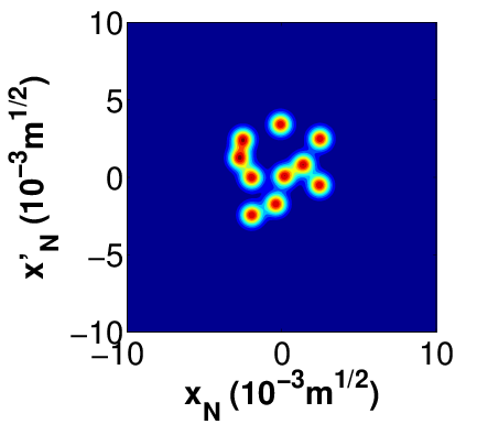
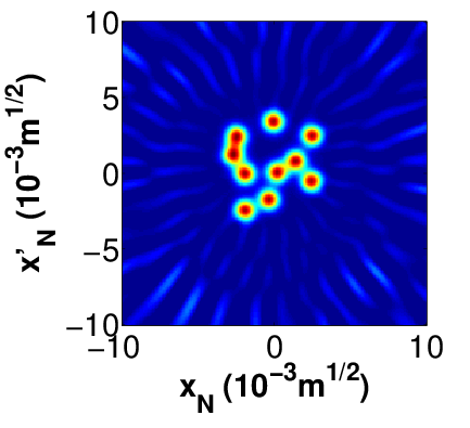
Figure 9: (a) Distribution in normalised phase space. (b) Reconstruction in normalised phase space.

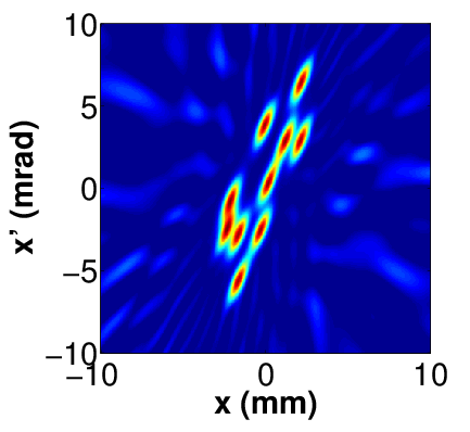
Figure 10: Distribution obtained by transforming the co-ordinates in the reconstruction in normalised phase space to the real phase space.

One way to transform from Fig. 9 to Fig. 10 is to make a square grid of pixel positions for Fig. (10), compute the corresponding positions in Fig. 9 using Eq. (68), then interpolate using the reconstructed Fig. 9. But there is a more direct way in which we can avoid the interpolation error. Recall that a reconstruction is computed using Eq. (16). Instead of using this to compute Fig. 9 first, we can use this to compute the distribution at coordinates in normalised phase space that correspond to the square grid in Fig. 10. In this way, Fig. 10 can be obtained directly from the projections.

We should mention that to use this method for quadrupole scan, the Twiss parameters at the reconstruction location must be measured first. This can be done using a standard method, e.g. as described in Ross or Castro . From experience, we find that the method is quite robust. For the method to provide some benefit in reconstruction and the applications described in the following sections, an estimate of the Twiss parameters is often sufficient.

VIII ALICE Tomography Section

In this section we describe the experimental setup at the tomography diagnostic section in the ALICE-to-EMMA injection line that we use for our measurements.

The full-energy electron beam in ALICE is typically varied between 10 MeV (for injection into EMMA) to 27 MeV (for FEL operation). In our experiments, we have only used 12 MeV. The tomography section consists of three YAG screens, with two quadrupoles in between each adjacent pair of screens, as shown in Fig. 11. The three screens are labelled 1 to 3. The electron beam travels in the direction from screen 1 to screen 3. The distance from screen 1 to screen 3 is 1.5 m. The quadrupoles of interest are labelled 7 to 11. The length - between the entrance and exit planes - of each of these quadrupoles is 50 mm. The quadrupole scans for our experiments are carried out using quadrupoles 7 and 10. We shall refer to these as QUAD-07 and QUAD-10 respectively. The other quadrupoles are all fixed at a current of 1.05 A during the scan.

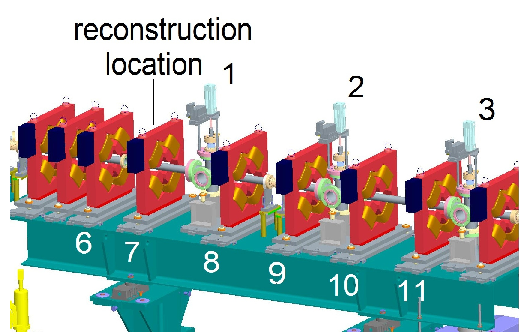
Figure 11: ALICE tomography section: The tomography diagnostic section of the ALICE-to-EMMA injection line.

Many factors influence the measurements. Figure 12 shows an image, taken by a camera (Pacific Board Cameras PC-375 Mono, 752x582 pixels, 8 bit) focused on screen 1 in Fig. 11, of a single bunch of charge of 20 pC. The size and shape of this image can be adjusted by changing the strength of QUAD-07, as well as all the other quadrupoles upstream of it. This is the feature that is used in a quadrupole scan. The size and shape of the image is also affected by day-to-day variation in the setup of ALICE, as well as shorter-term instabilities. This can lead to variation of the image from bunch to bunch. A quadrupole scan or a tomographic reconstruction makes use of a set of images, each taken at a slightly different time. The resulting emittance, Twiss parameters or reconstructed phase space derived from these images must therefore include some averaging of the bunch-to-bunch variations. Other variables include the response of the YAG screen and the response of the camera. We assume that the intensity recorded by the camera image is directly proportional to the number of electrons falling on each pixel.

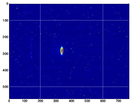
Figure 12: The image of the beam on screen 1. The ratio of distance on the screen to pixel size in the image is 0.0818 mm/pixel.

For tomographic measurements, the transfer functions of the quadrupoles must be known accurately. This requires knowledge of the magnetic field gradient in each quadrupole. We rely on field gradient versus current measurements provided by the manufacturer. Note that there is hysteresis in the quadrupole magnets; thus the field gradient can be slightly different, depending on the previous level of excitation. The hysteresis curve provided by the manufacturer shows that at one ampere current, the maximum error in the field is 7%. This error remains constant up to about 5 A, and is thus a potential source of measurement error.

The bunch charge used is in the range 20 to 80 pC, and the bunch repetition rate is a few hertz. We assume that when each bunch of electrons is incident on the screen, it produces luminescence proportional to the flux of electrons arriving at each point on the screen. The camera viewing the screen captures 50 images per second, but is not synchronised with the arrival of the electrons at the screen. During the analysis of the data we find a shot-to-shot variation in the brightness of 10 to 20%.

Although the ALICE tomography section was originally designed for tomographic measurements using three screens simultaneously, in practice it is time consuming to set up equal phase advances between screens. For this work, we have chosen to undertake the much quicker quadrupole scan method. The variation of quadrupole magnet currents and the capture of the corresponding camera images of the screens has been automated using software developed in-house. In a typical measurement, the strength of QUAD-07 is varied and the beam images on screen 1 are captured. The quadrupole field gradients are chosen to correspond to the required projection angles calculated using Eq. (19). The equation for the transfer map between the entrance to QUAD-07 to screen 1 is Eq. (14) The form of this function limits the angle range to about 160^∘. Typically, we record images at 1^∘ intervals, so 160 images would be collected.

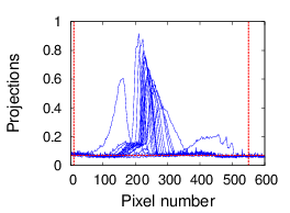
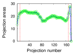
Figure 13: (a) Raw projections from the images of the QUAD-10 scan for 80 pC bunch charge. The horizontal line through the noise floor will be used as the new zero. (b) Integrated projection areas corresponding to the projection angles in Fig. 14. The dashed red lines mark the region outside of which the data is also excluded because integrated areas are well below the average. (The vertical axes of both graphs are in arbitrary units.)

Figure 13 shows examples of projections obtained directly from the images. We call these the raw projections. Before undertaking the quadrupole scan measurements, a dipole magnet before the quadrupole is adjusted to centre the beam on the screen, so that most of the projection peaks are at roughly the same position. The strength of the quadrupole which we intend to use for the measurements is then varied to check if the beam is also central in the magnet. If the beam is on the magnetic axis of the quadrupole, it will experience no force and the beam spot on the screen will not move. If the beam spot moves, we adjust beam steering upstream of the quadrupole magnet and check again. Notice for each projection that as we move away from its peak, the projection reaches a roughly constant, non-zero value. The background when there is no beam has also been measured and found to be close to the background when the beam is present. This background must be subtracted.

It is important to check the integrated area of each projection. Figure 13 is an example of the integrated areas calculated for a quadrupole scan. Note that the projection number corresponds to the projection angles in Fig. 14, which are taken at uniform intervals. As it can be seen in the figure, some of the projection areas are much smaller than the typical value. This happens when the beam becomes defocused, but why this happens is not understood at present. Including such projections could lead to errors, so they are omitted. This usually corresponds to the first and last few images for each of our quadrupole scan data sets. In the analyses following this section, the first and last ten projections are omitted, as indicated by the two vertical lines in Fig. 13. The trend in the area suggests that the bunch charge might have changed during the quadrupole scan.

IX Space Charge Search

IX.1 Space Charge Measurement Procedure

There is some simulation work on the effect of different bunch charges on the beam in ALICE Holder ; DArcy ; Holder2 . These publications suggest that at 80 pC bunch charge, changes in lattice functions and beamwidths become noticeable. If space charge effect is significant, it would have an impact on our tomographic reconstruction Stratakis2 . In order to determine if the space charge effect is significant, we design an experiment as follows.

A quadrupole scan is not by itself able to detect space charge effect. We propose to do it using two quadrupole scans that are separated by a distance that is much larger than the distance within a single scan. Our beam is likely to have a small space charge effect, if any. For each quadrupole scan, the distance between quadrupole and screen is small. Any space charge effect would be small, so errors need also to be small if any effect is to be observed. We then do two quadrupole scans at different positions. As the distance between the two scans is much larger than the distance within each scan, the space charge effect would also be much larger. It is by comparing the two scans that we hope to detect the space charge effect.

Quadrupole scans are carried out at screen 1 and screen 3, as shown in Fig. 11. These two screens are separated by 1.5 m. Using the beam images from either screen, the emittance could be obtained as described before. If the space charge effect is significant, the results from the two screens would be different. If there is indeed no space charge effect at all, the phase space reconstructed from the two scans should also be the same.

In order to obtain reasonable reconstructions, the parameters used in each quadrupole scan have to be selected to give a range of projection angles as close as possible to the full 180^∘. The reason is that the reconstruction can in theory be expressed as an integral of the filtered back projections over 180^∘ Kak . A reduced range would in effect be a truncation in angles. For direct comparison, we also require that, for both scans, the reconstruction be carried out at the same location.

The closest quadrupole in front of screen 1 is QUAD-07. We need to determine if this quadrupole could provide sufficient range in projection angles for the scan on screen 1. We choose as the common reconstruction location for both scans the entrance plane to QUAD-07. This same quadrupole would be used for the scan on screen 1. Between this location and screen 3, there are altogether five quadrupoles. We need to decide which one to choose for the scan on screen 3.

QUAD-07 is a horizontally focussing quadrupole. The region between the reconstruction location and screen 1 is made up of QUAD-07 followed by a drift space. Using the hard-edge model for the quadrupole, we can write down the transfer matrix from the reconstruction location to screen 1:

$$M=\left(\begin{array}[]{cc}1&L_{D}\\ 0&1\end{array}\right)\left(\begin{array}[]{cc}\cos(\omega L)&\sin(\omega L)/\omega\\ -\omega\sin(\omega L)&\cos(\omega L)\end{array}\right)$$ (93)

where $L$ is the quadrupole length, $L_{D}$ is the drift distance, and $\omega^{2}$ is the normalised quadrupole field gradient

$$k_{1}=\frac{e}{P_{0}}\frac{\partial B_{y}}{\partial x}.$$ (94)

Here, $e$ is the electron charge, $\partial B_{y}/\partial x$ is the magnetic field gradient and $P_{0}$ the electron momentum. The magnetic field gradient has been measured as a function of current $I$ by the manufacturer, and has the form

$$\frac{\partial B_{y}}{\partial x}=mI+d.$$ (95)

In the case of QUAD-07, for example, $m=1.5900$ T/m/A, and $d=0.0001$ T/m. These values are obtained by fitting a straight line to the numerical data provided by the manufacturer.

Using these equations, the projection angle $\theta$ can then be computed for each current using Eq. (19). A graph of the angle against current is plotted in Fig. 14. From this graph, the range of angles can be obtained.

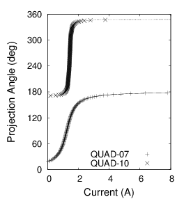
Figure 14: Projections angles versus QUAD-07 and QUAD-10 currents at 12 MeV.

We have seen that the QUAD-07 scan for screen 1 gives a fairly wide range of angles, from about 20^∘ to 170^∘, which should be sufficient for our purpose.

We turn now to the scan for screen 3. In order to have a good, well focussed beam on the screen, all of the quadrupoles from QUAD-07 to QUAD-11 must be on. One of these must then be selected. Only QUAD-10 has a stable range that is close to 180^∘. The range at 12 MeV is plotted in Fig. 14. There is a very steep slope that covers a large part of the range of angles, for a small interval of currents. This suggests that a small error in current could lead to a large error in angle.

IX.2 Tomographic Reconstructions

The reconstructions for the QUAD-07 and QUAD-10 scans are shown in Fig. 15 for two bunch charges, 20 pC and 80 pC. As explained in section IX.1, the experiment is designed in such a way as to give nominally identical reconstructions for both scans, at the entrance face to QUAD-07 - when there is no space charge effect. Figure 15 looks different from Fig. 15, and Fig. 15 looks different from Fig. 15. If the space charge has a linear effect, this could happen. For instance, if the space charge defocuses the beam in the same way as a defocussing quadrupole (both horizontally and vertically), this would be a linear effect. Errors in quadrupole gradients and bunch to bunch variations are also possible causes. It is straightforward to estimate the effects of quadrupole gradient errors, which we now do. The estimation could be viewed as a result of either the linear defocusing effect of space charge, or the gradient errors, or a combination of both.

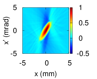
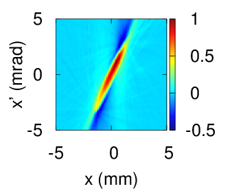
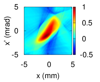
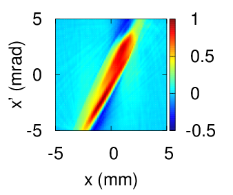
Figure 15: Reconstruction at entrance face of QUAD-07 with bunch charges of: 20 pC for (a) QUAD-07 and (b) QUAD-10 scans; 80 pC for (c) QUAD-07 and (d) QUAD-10 scans.

An error in the field gradient of the quadrupole could come from an error in the current setting, or an error in the calibration in Eq. (95). For our purpose, we shall combine the two effects into a current error. An error in the current would lead to an error in the transfer matrix, such as Eq. (93) for the QUAD-07 scan. The result would be a reconstructed distribution that looks different from the actual one. However, the two distributions would be related by a linear transfer matrix. Assuming that current error is the cause, if we transform both reconstructions of the QUAD-07 and QUAD-10 scans to normalised phase space, the resulting distribution should look the same, differing by a simple rotation at most. The procedure for doing so is described in Hock . It requires an estimate of the Twiss parameters, which are obtained in the next section. The resulting normalised phase space distributions are shown in Fig. 16. We first summarise the procedure.

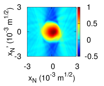
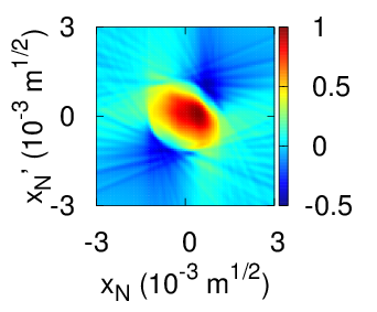
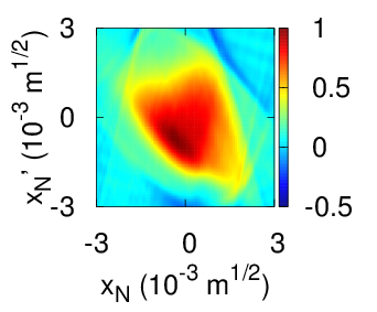
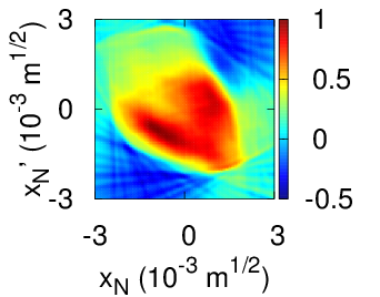
Figure 16: Normalised phase space at entrance face of QUAD-07 with bunch charges: 20 pC for (a) QUAD-07 and (b) QUAD-10 scans; 80 pC for (c) QUAD-07 and (d) QUAD-10 scans.

The implementation of the Filtered Back Projection technique normally assumes that the intervals of angles are uniform Kak . In Eq. 56, we have given a formula that is suitable for nonuniform intervals of angles. This would be useful later, when we consider the effect of an error in the quadrupole current.

To reconstruct in normalised phase space, we first define a rectangular grid of the co-ordinates $(x_{N},x_{N}^{\prime})$, calculate the corresponding co-ordinates in real space using:

$$\left(\begin{array}[]{c}x\\ x^{\prime}\end{array}\right)=\left(\begin{array}[]{cc}\sqrt{\beta}&0\\ -\frac{\alpha}{\sqrt{\beta}}&\frac{1}{\sqrt{\beta}}\end{array}\right)\left(\begin{array}[]{c}x_{N}\\ x^{\prime}_{N}\end{array}\right),$$ (96)

where $\alpha$ and $\beta$ are the Twiss parameters, then reconstruct using Eq. (56).

The structures in the phase space distributions are more clearly visible in the normalised phase space in Fig. 16, than in the real phase space in Fig. 15. The structures in Figs. 16 and 16 look similar, except that 16 looks stretched. This could be due to errors in the measured Twiss parameters. Next, look at Figs. 16 and 16. Both reveal similar, heart-shaped distributions, with one rotated with respect to the other. A rotation is what we would expect from an error in the transfer matrix, which could arise from errors in current or field gradient. As a simple test, we repeat the reconstruction of Fig. 16 from the projections. The procedure requires the computing of the transfer matrix from the entrance face of QUAD-07 to screen 3. This relies on the calibration of Eq. (95) for each of the intervening quadrupoles. This time, we add an error of +0.3 A to the current settings recorded in the experiment for QUAD-10. The transfer matrix calculated from this new set of currents give angles that follow the same QUAD-10 curve in Fig. 14. A positive current error would cause the points to move upwards, suggesting that some form of rotation may take place.

An important step has to be taken before the reconstruction can take place correctly. The intervals of angle for QUAD-10 in Fig. 14 are no longer uniform. This change must be applied to $\Delta\theta_{k}$ in Eq. (56) as weighting factors. As demonstrated in Hock , a sum of half of the angular intervals on the two sides of each projection works well. In this set of data, we do not have the full range of angles of 180^∘. So for the first projection, the factor would be half of the interval between the angles of the first two projections only. Likewise for the last projection. This choice maintains the equivalence of Eq. (56) to the trapezium rule of integration that is explained in Hock .

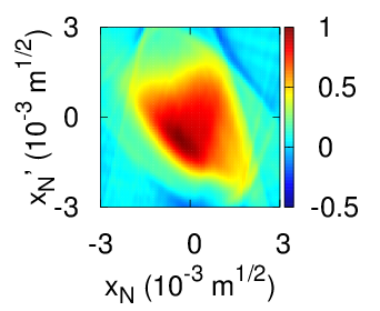
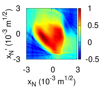
Figure 17: 80 pC, normalised phase space: (a) reconstruction for the QUAD-07 scan; (b) reconstruction for the QUAD-10 scan, assuming a current error of +0.3 A.

Following Eqs. (56) and (68), we reconstruct the normalised phase space in Fig. 17. This is clearly rotated with respect to the original Fig. 16. It is now at roughly the same orientation as the screen 1 result Fig. 16, reproduced in Fig. 17 for direct comparison. The similarity shows that the two quadrupole scans give consistent results. As these are taken at different positions along the beamline, the similarity also provides support that the reconstructed phase space distribution is correct.

This suggests that an error in quadrupole field or current could contribute to the difference between the screen 1 result in Fig. 15, and the screen 3 result in Fig. 15. A current error 0.3 A seems rather large. Other reasons may include fringe fields and space charge. Further study is needed to confirm this.

X MENT Reconstructions

MENT can be used for tomographic reonstructions when the number of projections is small. At ALICE, PITZ, SNS and PSI, 3 to 5 projections are used Reggiani . In contrast, we could for example collect over 100 projections using quadrupole scans and reconstruct using FBP. With so few projections in MENT, it is not clear how reliable the reconstructions are. We review here our study Hock1 which shows that the reconstructions are sensitive to the actual projection angles selected and can be highly distorted, and that by using equal angle intervals in normalised phase space - i.e. equal phase advances - distortion can be reduced significantly.

X.1 Distortions

As an example of a more complex distribution, we choose a hypothetical distribution with a number of Gaussian spots, as shown in Fig. 18. We use this as a test case to compare the results of the two methods for choosing projection angles. Figure 18 is the result of reconstructing with 5 projections at equal angular intervals in real phase space. The result is very sensitive to the actual directions of the five angles. The result shown here is the worst case, where the individual spots are not resolved. The best case shown in Fig. 18 is obtained when the rays are all rotated by half an angle interval, actually agrees very well with the original in Fig. 18.

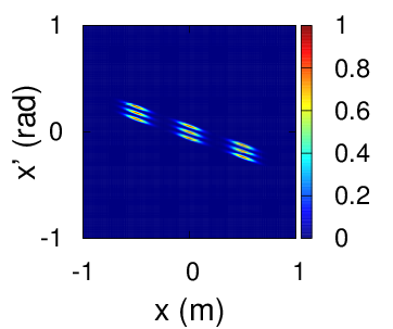
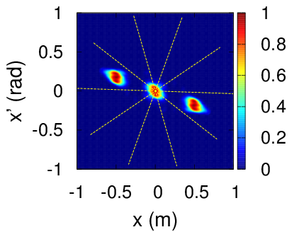
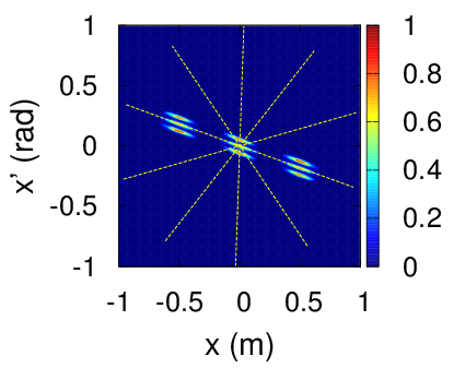
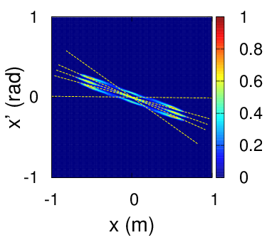
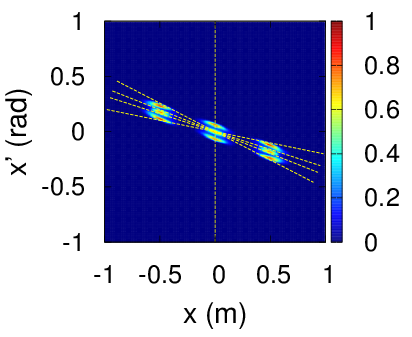
Figure 18: (a) Original distribution, with 9 spots; (b) reconstructed using 5 projections at equal angular intervals in real phase space, with yellow lines showing ray directions; (c) the same, but with projection angles rotated half an interval; (d) reconstructed using 5 projections at equal phase advances, with yellow lines showing ray directions; (e) the same, but with projection angles rotated half an interval in normalised phase space.

We now apply the method of equal phase advances, i.e. we use equal angles in normalised phase space. The result is shown in Fig. 18. This is much closer to the original than Fig. 18, though not as good as Fig. 18. Notice that when equal phase advances are chosen, the corresponding rays in real phase space are closely bunched along the length of the distribution. This means more samples within the angular range of the distribution, where it really matters. This is clear from the yellow lines in Fig. 18.

If the normalised phase space angles in Fig. 18 are changed by half an interval, it would give Fig. 18. This is slightly clearer, though still not as good as Fig. 18. So using equal phase advances give consistently reliable results, whereas using equal angle intervals in real phase space could give highly distorted results for some angles.

These simulation results show that we must be careful when interpreting MENT results because significant distortions are possible. They also provide a visual explanation for the conclusion that 45^∘ phase advances give minimum emittance error in the 4 screen setup in Castro . It is because the angular distribution is sampled optimally.

X.2 Re-analysing FBP Data

Implementing equal phase advances on a beamline is possible with some effort. At PITZ, equal phase advances are set up before measurements Asova2 by adjusting upstream magnets to match the beam distribution into the periodic Twiss parameters at the tomography section. At ALICE, this set up has not been attempted.

For this analysis, we shall obtain these phase advances in a simple way from measured data. In our previous work at ALICE, we have reported a comprehensive set of phase space measurements Ibison . The projections are obtained with quadrupole scans and the phase space is reconstructed using FBP. The basic setup consists of only one screen and one quadrupole. As the strength of the quadrupole is varied, a camera captures the image on the screen repeatedly. The procedure is automated by a computer and each scan of the quadrupole strength can be completed in about 10 minutes. In a typical measurement, over 100 projections at 1^∘ intervals are obtained. For this analysis, we simply pick out a few angles from this set of projections that correspond to equal phase advances. Then we reconstruct the phase space using MENT.

Instead of having 3 to 5 screens and quite a number of quadrupoles, as is typical in beamlines designed to use MENT, all we need is 1 screen and 1 quadrupole. It may seem redundant to use MENT for reconstruction if we can reconstruct the phase space using FBP. However, there are a few good reasons:

1. A single quadrupole cannot give the full range of projection angles Ibison , so the FBP result tends to have streaking artefacts.

2. MENT could produce clean results with no artefacts. (Whether or not it is distorted is a question we seek to answer.)

3. Using the quadrupole scan to obtain projections needed for MENT is very quick and requires far less hardware compared to the standard procedure of using 3 to 5 screens.

4. Having an alternative method to measure the phase space is useful because it provides a check for consistency. The MENT result could be compared with the FBP result.

We select experimental data from the measurement of a beam at ALICE with 80 pC bunch charge. The measurement setup has been reported in Ibison . Here, we shall assume that the projections have been measured. The distribution has been reconstructed with FBP, as shown in Fig. 19.

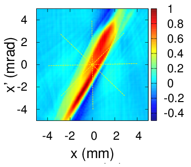
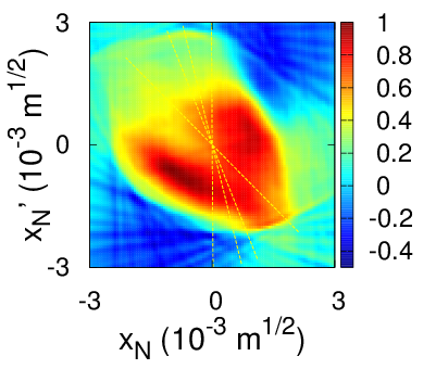
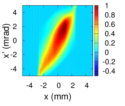
Figure 19: (a) FBP reconstruction, with yellow lines showing ray directions for equal angular intervals in real phase space; (b) the same distribution and rays, transformed to normalised phase space; (c) reconstructed using the 4 projections with MENT.

With the projections from the quadrupole scan, we can estimate the Twiss parameters using the method in Ross . With a knowledge of the Twiss parameters, we can then transform the distribution to normalised phase space, as shown in Fig. 19. To apply MENT, we first try it for the case of projections with equal angular intervals. We pick out 4 angles, as shown by the yellow lines in Fig. 19. We must be careful to skip over the gap that is not covered by the range of projection angles that is possible with a single quadrupole. The corresponding rays in normalised phase space are shown by the yellow lines in Fig. 19. They are now bunched into a small range of angles. Applying MENT to these projections, we get Fig. 19. This is clearly broader and apparently distorted when compared with Fig. 19. However, we should reserve judgement at this stage because we know that Fig. 19 is also not perfect.

Next, we apply the method of equal phase advances. We know from Hock that this means equal angles in normalised phase space. So we pick four angles in normalised phase space, as shown by the yellow lines in Fig. 20. Again, we must be careful to skip over the gap in the angular range. (If the gap is too large, fewer projections would be possible and the experiment might have to be redesigned. This could mean changing the quadrupole’s strength and its distance from the screen to increase the range of projection angles.) The corresponding angles in real phase space are shown by yellow lines in Fig. 20. Notice that they are bunched closer to the length of the FBP distribution. The projections are reconstructed with MENT. The result in Fig. 20 clearly shows better agreement with the FBP result than Fig. 19.

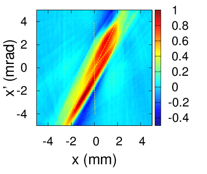
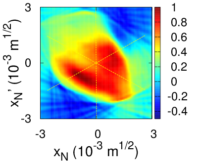
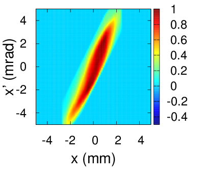
Figure 20: (a) FBP reconstruction, with yellow lines showing ray directions for equal phase advances; (b) the same distribution and rays, transformed to normalised phase space; (c) reconstructed using the 4 projections with MENT.

This demonstration provides support for the the method of equal phase advance. It also suggests that quadrupole scan is a possible setup in which we could use MENT with the method of equal phase advance.

XI Conclusion

We have presented a coherent view of the normalised phase space method for phase space tomography:

1. In 2003, a method to measure emittance at the Tesla Test Facility 2 is developed Castro . The method uses 4 screens. Adjacent screens are separated by identical FODO cells. Simulations show that statistical errors in emittance measurements are minismised by choosing a setup in which phase advance is 45^∘ between adjacent screens.

2. In 2007, this idea is used to design the PITZ tomography section Asova . The 45^∘ value is now associated with 180^∘ divided by 4, the number of screens. The 180^∘ is in turn associated with the full range of projection angles in a tomographic measurement. The reason for this association is not explained, but the use of 45^∘ phase advance is justified using the emittance measurement method as in Castro . In this way, the idea that equal phase advances is optimal for tomographic measurement is first proposed.

3. In 2008, the idea of equal phase advance is applied to the design of the ALICE tomography section Muratori . This time, the idea is used directly without the justification of emittance measurement.

4. In 2010, both the PITZ tomography section Asova2 and the ALICE tomography section Muratori2 are commissioned. Subsequent tomographic measurements at PITZ has followed closely a procedure to setup equal phase advances Asova2 . At the ALICE, beam time dedicated to tomographic measurement has been limited. Instead, quick quadrupole scans are used without any phase advance setup.

5. In 2011, we supply the justification for equal phase advance by showing that it is equal to the projection angle in a normalised phase space Hock . In this phase space, the distribution is circular on average, and equal intervals of projection angles become an optimal choice.

6. Since then, we have applied the idea of equal phase advances to improve resolution in FBP reconstructions Hock , detect linear errors in a beamline Ibison and improve reliability in MENT reconstructions Hock1 . We plan to apply this to improve resolution and reliability in 4D reconstruction where the number of projections that can be measured is likely to be limited by measurement time Hock2 .

- (1) D. Stratakis, et al, “Phase space tomography of beams with extreme space charge”, Proc. PAC07, Albuquerque, New Mexico, USA (2007).
- (2) C. B. McKee, P. G. O’Shea, J. M. J. Madey, Nuclear Instruments and Methods in Physics Research A 358, 764 (1995).
- (3) G. Asova, et al, “First results with tomographic reconstruction of the transverse phase space aat PITZ”, Proceedings of FEL2011, Shanghai, China (2011).
- (4) D. Stratakis, et al, “Tomography as a diagnostic tool for phase space mapping of intense particle beams”, Phys. Rev. Spec. Top. Acceler. Beams 9 (2006) 122801.
- (5) D. Reggiani, et al, “Transverse phase-space beam tomography at PSI and SNS proton accelerators”, Proc. IPAC10, Kyoto, Japan (2010).
- (6) Phase space tomography, http://tomograp.web.cern.ch/tomograp/
- (7) K. Honkavaara, et al, “Electron beam characterization at PITZ and the VUV-FEL at DESY”, FEL 2005, Stanford.
- (8) V. Yakimenko, et al, “Electron beam phase-space measurement using a high-precision tomography technique”, Phys. Rev. ST Accel. Beams 6, 122801 (2003).
- (9) Y.-N. Rao and R. Baartman, “Transverse phase space tomography in TRIUMF injection beamline”, Proceedings of IPAC2011, San Sebastian, Spain, pp. 1144-1146.
- (10) M. G. Ibison, et al, “ALICE Tomography Section: Measurements and Analysis”, Journal of Instrumentation, 7, P04016 (2012).
- (11) S. Y. Lee, Accelerator Physics, 2nd ed., World Scientific, Singapore (2007), p. 53.
- (12) G. Asova, et al, “Design consideration for phase space tomography diagnostics at the PITZ facility”, Proc. DIPAC 2007, Venice, Italy (2007).
- (13) B.D. Muratori, et al, “Injection and extraction for the EMMA NS-FFAG”, Proceedings of EPAC08, Genoa, Italy (2008).
- (14) B.D. Muratori, et al, “Preparations for EMMA Commissioning”, Proceedings of IPAC10, Kyoto. Japan (2010).
- (15) G. Asova, et al, “Phase space tomography diagnostics at the PITZ facility,” Proc. ICAP 2006, Chamonix, France.
- (16) K. M. Hock, et al, “Beam tomography in transverse normalised phase space”, Nucl. Instr. and Meth. A, 642, (2011), pp. 36-44.
- (17) K. M. Hock and M. G. Ibison, “A study of the Maximum Entropy Technique for phase space tomography”, Journal of Instrumentation, 8, P02003 (2013).
- (18) M. G. Ibison, et al, “ALICE Tomography Section: Measurements and Analysis”, Journal of Instrumentation, 7, P04016 (2012).
- (19) A.C. Kak and M. Slaney, Principles of Computerized Tomographic Imaging, (SIAM, Philadelphia, USA, 2001), pp. 60-75. http://www.slaney.org/pct/pct-toc.html Accessed on 8 Aug 2013.
- (20) C. T. Mottershead, “Maximum entropy beam diagnostic tomography”, IEEE Transactions on Nuclear Science, NS-32, (1985), pp. 1970-1972.
- (21) A. M. Glazer and J. S. Wark, Statistical Mechanics: A Survival Guide, OUP Oxford, 2001, pp. 14-16.
- (22) A.C. Kak and M. Slaney, Principles of Computerized Tomographic Imaging, (SIAM, Philadelphia, USA, 2001), pp. 60-75. http://www.slaney.org/pct/pct-toc.html Accessed on 8 Aug 2013.
- (23) P. Castro, “Monte Carlo Simulations of emittance measurements at TTF2”, DESY Technical Note 03-03, 2003.
- (24) D.J. Holder and B.D. Muratori, “Modelling the ALICE electron beam properties through the EMMA Injection Line Tomography Section”, Proc. PAC09, Vancouver, Canada (2009).
- (25) F. Loehl, “Measurements of the Transverse Emittance at the VUV-FEL”, DESY, Hamburg (2005). http://gan.desy.de/floehl/DiplomaThesis/DESY-THESIS_2005-014_gray.pdf Accessed on 8 Aug 2013.
- (26) M. C. Ross, N. Phinney and G. Quickfall, “Automated emittance measurements in the SLC”, Proceedings of the Particle Accelerator Conferences 1987, pp. 725 - 728.
- (27) R. T. P. D’Arcy, et al, “Modelling of the EMMA NS-FFAG injection line using GPT”, Proceedings of IPAC10, Kyoto, Japan, 2010.
- (28) D.J. Holder, et al, “A phase space tomography diagnostic for PITZ”, Proceedings of EPAC, Edinburgh, UK (2006).
- (29) K. M. Hock and A. Wolski, “Tomographic reconstruction of the full 4D transverse phase space”, Nuclear Instruments and Methods A, vol. 726, (2013), pp. 8 16.