A mean-field monomer-dimer model with attractive interaction. The exact solution.

Abstract

A mean-field monomer-dimer model which includes an attractive interaction among both monomers and dimers is introduced and its exact solution rigorously derived. The Heilmann-Lieb method for the pure hard-core interacting case is used to compute upper and lower bounds for the pressure. The bounds are shown to coincide in the thermodynamic limit for a suitable choice of the monomer density $m$. The consistency equation characterising $m$ is studied in the phase space $(h,J)$, where $h$ tunes the monomer potential and $J$ the attractive potential. The critical point and exponents are computed and show that the model is in the mean-field ferromagnetic universality class.

I Introduction and results

Each way to fully cover the vertices of a finite graph $G$ by non-overlapping dimers (molecules which occupy two adjacent vertices) and monomers (molecules which occupy a single vertex) is called a monomer-dimer configuration. Associating to each of those configurations a probability proportional to the product of a factor $w>0$ for each dimer and a factor $x>0$ for each monomer defines a monomer-dimer model with pure hard-core interaction.

Those models were proposed to investigate the properties of diatomic oxygen molecules deposited on tungstenR or to study liquid mixtures in which the molecules are unequal in sizeFR . The hard-core interaction accounts for the contact repulsion generated by the Pauli principle. In order to account also for the attractive component of the Van der Waals potential among monomers and dimers, one may consider an attractive interactionRM ; Ch ; Chcambr among particles occupying neighbouring sites (as it was previously done for single atomsF ; Pe ).

More recently monomer-dimer models on diluted network have attracted a considerable attentionmz ; ac and they have been applied, with the addition of a ferromagnetic imitative interaction, also in social sciencesimm .

The partition function describing a general system of interacting monomers and dimers can be written as

$$Z_{G}\;=\;\sum_{D\in\mathscr{D}_{G}}x^{M}w^{|D|}z_{1}^{I_{m}}z_{2}^{I_{d}}z_{3}^{I_{md}}\;,$$ (1)

where $z_{1},z_{2},z_{3}>0$ tune the interaction among particles and for a given dimer configuration $D$, $M$ is the corresponding number of monomers, $I_{m}$ the number of neighbouring monomers, $I_{d}$ the number of neighbouring dimers, $I_{md}$ the number of neighbouring molecules of different type.

In this paper we investigate a system where the attraction among monomers and among dimers is stronger than the attraction among molecules of different type, that is $z_{1}z_{2}\geq z_{3}^{2}$. And precisely we study the mean-field case, i.e. the model on the complete graph where each of the $N$ sites is connected with all the others and the particle system is permutation invariant. Considering the relation $2|D|+M=N$ induced by the hard-core interaction among particles, we may study without loss of generality a reduced model given by the parametrisation $x=e^{h}$, $w=1/N$, $z_{1}=z_{2}=e^{J/N}$, $z_{3}=1$. We prove that, at large volumes, the model turns out to be described by the monomer density $m(h,J)$, i.e. the expectation value, with respect to the probability measure introduced by (1), of the fraction of sites occupied by monomers.

For pure hard-core interactions, i.e. $J=0$, Heilmann and Lieb HL ; HLprl proved the absence of phase transitions for both regular lattices and in the mean-field case (complete graph) treated here. Using the relation between the partition function and the Hermite polynomials, we compute here the thermodynamic limit of the free energy in the pure hard-core case and use it to solve the attractive case by means of a one-dimensional variational principle in the monomer density. For a suitable smooth, monotonic, function $g$ mapping $\mathbb{R}$ into the interval $(0,1)$, we find that $m(h,J)$ can be identified among the solutions (at most three) of the consistency equation

$$m=g((2m-1)J+h)$$ (2)

characterising the entire phase space of the model. In particular it turns out that $m$ has, in the $(h,J)$ plane, a jump discontinuity on a curve $h=\gamma(J)$. The curve $\gamma$, implicitly defined, stems at

$$(h_{c},J_{c})\;=\;\left(\frac{1}{2}\,\log(2\sqrt{2}-2)-\frac{1}{4}\,,\,\frac{1}{4\,(3-2\sqrt{2})}\right)\,,$$ (3)

is smooth outside the critical point $(h_{c},J_{c})$ and at least differentiable approaching it, moreover is has an asymptote at $h=-1/2$ for large values of $J$. The order parameter $m(h,J)$ is characterised in a neighbourhood of the critical point by the mean-field theory critical exponents: $\boldsymbol{\beta}=1/2$ along the direction of $\gamma$, and $\boldsymbol{\delta}=3$ along any other direction of the plane $(h,J)$.

The paper is organised as follows: in Section II we introduce and solve the model without attraction following the methods of Heilmann and Lieb. In Section III we introduce the model with attractive interaction and we show how to control the thermodynamic limit of the free energy by means of a one dimensional variational problem. Section IV presents the study of the consistency equation (2) in the $(h,J)$ plane, contains the study of the implicit equation for the curve $\gamma$ and the computation of critical exponents of the model. The Appendix contains supplementary material of elementary type that makes the paper self-contained.

II Monomer-dimer model

Let $G=(V,E)$ be a finite simple graph with vertex set $V$ and edge set $E\subseteq\{uv\equiv\{u,v\}\,|\,u\neq v\in V\}\,$.

Definition 1.

A dimer configuration $D$ on the graph $G$ is a set of pairwise non-incident edges (called dimers):

$$D\subseteq E\quad\text{and}\quad\big{(}uv\in D\ \Rightarrow\ uw\notin D\ \forall w\neq v\big{)}\,.$$

Given $D$, the associated monomer configuration is the set of dimer-free vertices (called monomers):

$$\mathscr{M}(D):=\mathscr{M}_{G}(D):=\{u\in V\,|\,uv\notin D\ \forall v\in V\}\,.$$

Notice that $|\mathscr{M}(D)|+2\,|D|=|V|\,$.

Definition 2.

Let $\mathscr{D}_{G}$ be the set of all possible dimer configurations on the graph $G\,$. The monomer-dimer model on $G$ is obtained by assigning a monomer weight $x_{v}>0$ to each vertex $v\in V$ and a dimer weight $w_{e}>0$ to each edge $e\in E$ and considering the following probability measure on the set $\mathscr{D}_{G}$:

$$\mu^{\textup{\tiny{MD}}}_{G}(D)=\frac{1}{Z^{\textup{\tiny{MD}}}_{G}(\mathbf{x},\mathbf{w})}\;\textstyle\prod_{e\,\in D}w_{e}\,\textstyle\prod_{v\,\in\mathscr{M}(D)}x_{v}\quad\forall\,D\in\mathscr{D}_{G}\,.$$

The normalising factor, called partition function of the model, is

$$Z^{\textup{\tiny{MD}}}_{G}(\mathbf{x},\mathbf{w}):=\sum_{D\in\mathscr{D}_{G}}\,\textstyle\prod_{e\,\in D}w_{e}\,\textstyle\prod_{v\,\in\mathscr{M}(D)}x_{v}$$ (4)

Its natural logarithm $\log Z^{\textup{\tiny{MD}}}_{G}$ is called pressure.

Remark 1.

If uniform dimer (resp. monomer) weights are considered, i.e. $w_{e}\equiv w\;\forall e\in E$ (resp. $x_{v}\equiv x\;\forall v\in V$), then it’s possible to keep $w=w_{0}$ (resp. $x=x_{0}$) fixed and study only the dependence of the model on $\mathbf{x}$ (resp. $\mathbf{w}$) without loss of generality. Indeed, using the relation $|\mathscr{M}(D)|+2\,|D|=|V|\,$, it’s easy to check that

$$Z^{\textup{\tiny{MD}}}_{G}(\mathbf{x},w)\,=\,(w/w_{0})^{|V|/2}\;Z^{\textup{\tiny{MD}}}_{G}\big{(}\frac{\mathbf{x}}{(w/w_{0})^{1/2}}\,,\,w_{0}\big{)}\;;$$ (5)

$$Z^{\textup{\tiny{MD}}}_{G}(x,\mathbf{w})\,=\,(x/x_{0})^{|V|}\;Z^{\textup{\tiny{MD}}}_{G}\big{(}x_{0}\,,\frac{\mathbf{w}}{(x/x_{0})^{2}}\big{)}\;.$$ (6)

Remark 2.

With uniform monomer weights, a direct computation shows that the monomer density, i.e. the expected fraction of monomers on the graph, is related to the derivative of the pressure w.r.t. $x\,$:

$$m^{\textup{\tiny{MD}}}_{G}:=\sum_{D\in\mathscr{D}_{G}}\frac{|\mathscr{M}(D)|}{|V|}\;\mu^{\textup{\tiny{MD}}}_{G}(D)\,=\,x\,\frac{\partial}{\partial x}\frac{\log Z^{\textup{\tiny{MD}}}_{G}}{|V|}\,.$$

Remark 3.

With bounded monomer and dimer weights $\underline{x}\leq x_{v}\leq\overline{x}$, $w_{e}\leq\overline{w}$, the following bounds for the pressure hold:

$$\log\underline{x}\,\leq\,\frac{\log Z^{\textup{\tiny{MD}}}_{G}(\mathbf{x},\mathbf{w})}{|V|}\,\leq\,\log\overline{x}+\frac{|E|}{|V|}\,\log\big{(}1+\frac{\overline{w}}{\overline{x}^{2}}\,\big{)}\,.$$

Proof.

The lower bound is obtained from (4) considering only the empty dimer configuration (i.e. a monomer on each vertex of the graph):

$$Z^{\textup{\tiny{MD}}}_{G}\,\geq\,\prod_{v\in V}x_{v}\,\geq\,\underline{x}^{|V|}\,.$$

The upper bound is obtained from (4) using the fact that any dimer configuration made of $d$ dimers is a (particular) set of $d$ edges:

$$\begin{split}Z^{\textup{\tiny{MD}}}_{G}\,&\leq\,\sum_{d=0}^{|E|}\textit{Card}\{D\in\mathscr{D}_{G}\,,\,|D|=d\}\;\overline{w}^{d}\;\overline{x}^{|V|-2d}\,\leq\,\sum_{d=0}^{|E|}{|E|\choose d}\,\overline{w}^{d}\;\overline{x}^{|V|-2d}\,=\\ &=\,\overline{x}^{|V|}\,(1+\overline{w}\,\overline{x}^{-2})^{|E|}\;.\qed\end{split}$$

The following recursion for the partition function, due to Heilmann and Lieb HL , is a fundamental property of the monomer-dimer model.

Proposition 1.

Given a vertex $o$ and its neighbours $v$, it holds

$$Z^{\textup{\tiny{MD}}}_{G}(\mathbf{x},\mathbf{w})\,=\,x_{o}\,Z^{\textup{\tiny{MD}}}_{G-o}(\mathbf{x}^{\prime},\mathbf{w}^{\prime})\,+\,\sum_{v\sim o}\,w_{ov}\,Z^{\textup{\tiny{MD}}}_{G-o-v}(\mathbf{x}^{\prime\prime},\mathbf{w}^{\prime\prime})\;,$$

where $\mathbf{x}^{\prime},\mathbf{w}^{\prime},\mathbf{x}^{\prime\prime},\mathbf{w}^{\prime\prime}$ are the weights vectors conveniently restricted to the involved subgraphs.

Proof.

The dimer configurations on $G$ having a monomer on the vertex $o$ coincide with the dimer configurations on $G-o$. Instead the dimer configurations on $G$ having a dimer on the edge $ov$ are in one-to-one correspondence with the dimer configurations on $G-o-v$. Therefore

$$\begin{split}Z^{\textup{\tiny{MD}}}_{G}\,&=\,\displaystyle\sum_{D\in\mathscr{D}_{G}}\textstyle\prod_{e\,\in D}w_{e}\,\textstyle\prod_{v\,\in\mathscr{M}_{G}(D)}x_{v}\\ &=\displaystyle\sum_{D\in\mathscr{D}_{G},\atop o\in\mathscr{M}_{G}(D)}\!\!\!\!\textstyle\prod_{e\,\in D}w_{e}\,\textstyle\prod_{v\,\in\mathscr{M}_{G}(D)}x_{v}\,+\,\displaystyle\sum_{v\sim o}\displaystyle\sum_{D\in\mathscr{D}_{G},\atop ov\in D}\!\!\textstyle\prod_{e\,\in D}w_{e}\,\textstyle\prod_{v\,\in\mathscr{M}_{G}(D)}x_{v}\\ &=\,x_{o}\!\!\displaystyle\sum_{D\in\mathscr{D}_{G-o}}\!\!\!\textstyle\prod_{e\,\in D}w_{e}\,\textstyle\prod_{v\,\in\mathscr{M}_{G-o}(D)}x_{v}\,+\,\displaystyle\sum_{v\sim o}\,w_{ov}\!\!\!\!\!\!\displaystyle\sum_{\ \ D\in\mathscr{D}_{G-o-v}}\!\!\!\!\!\!\!\!\textstyle\prod_{e\,\in D}w_{e}\,\textstyle\prod_{v\,\in\mathscr{M}_{G-o-v}(D)}x_{v}\\ &\,=\,x_{o}\,Z^{\textup{\tiny{MD}}}_{G-o}\,+\,\displaystyle\sum_{v\sim o}w_{ov}\,Z^{\textup{\tiny{MD}}}_{G-o-v}\;.\hskip 217.0pt\qed\end{split}$$

II.1 The monomer-dimer model on the complete graph

Let $K_{N}=(V_{N},E_{N})$ be the complete graph over $N$ vertices, that is $V_{N}=\{1,\dots,N\},\ E_{N}=\{uv\,|\,u,v\in V_{N},\,u<v\}$. Notice $|E_{N}|=N(N-1)/2$.
We work with uniform weights and we want $\log Z^{\textup{\tiny{MD}}}_{K_{N}}\,=\,\mathcal{O}(N)$. For this purpose, observing remark 3, we have to choose $x,\,w$ such that $w/x^{2}=\mathcal{O}(1/N)$. By remark 1 we can fix without loss of generality $w=1/N$ and study

$$Z^{\textup{\tiny{MD}}}_{N}(x)\,:=\,Z^{\textup{\tiny{MD}}}_{K_{N}}\big{(}x\,,\frac{1}{N}\,\big{)}\,,$$ (7)

indeed choosing $w_{0}=1/N$ in (5) it’s easy to check that $Z^{\textup{\tiny{MD}}}_{K_{N}}(x,w)=(wN)^{N/2}\,Z^{\textup{\tiny{MD}}}_{N}(c^{-1/2})$ whenever $w/x^{2}=c/N$. Observe that the bounds of remark 3 become

$$\log x\,\leq\,\frac{\log Z^{\textup{\tiny{MD}}}_{N}(x)}{N}\,\leq\,\log x+\frac{N-1}{2}\,\log\big{(}1+\frac{1}{Nx^{2}}\,\big{)}\,\leq\,\log x+\frac{1}{2\,x^{2}}\,.$$

On the complete graph it is possible to compute explicitly the partition function and it turns out to be related to the Hermite polynomials. We will give two proofs: the first one due to Heilmann and Lieb HL is based on a recurrence relation and applies also to other graphs, the second one is based on a simple combinatorial argument.

Theorem 1.

The partition function of the monomer-dimer model on the complete graph $K_{N}$ is

$$Z^{\textup{\tiny{MD}}}_{N}(x)\,=\,\big{(}\frac{i}{\sqrt{N}}\,\big{)}^{N}\;H_{N}\big{(}\!-i\,x\sqrt{N}\,\big{)}\;,$$

where $H_{N}$ denotes the $N^{th}\!$ probabilistic Hermite polynomial.

First proof.

Use the Heilmann-Lieb recursion of proposition 1 with $o=N$

$$Z^{\textup{\tiny{MD}}}_{K_{N}}(x,1)\,=\,x\,Z^{\textup{\tiny{MD}}}_{K_{N}-N}(x,1)\,+\,\sum_{v=1}^{N-1}Z^{\textup{\tiny{MD}}}_{K_{N}-N-v}(x,1)\,;$$

then observe that for any $u,\,v\in V_{N}$ the graphs $K_{N}-u$, $K_{N}-u-v$ are isomorphic to $K_{N-1}$, $K_{N-2}$ respectively and complete with the initial conditions:

$$\left\{\begin{array}[]{l}Z^{\textup{\tiny{MD}}}_{K_{N}}(x,1)\,=\,x\,Z^{\textup{\tiny{MD}}}_{K_{N-1}}(x,1)\,+\,(N-1)\,Z^{\textup{\tiny{MD}}}_{K_{N-2}}(x,1)\\[4.0pt] Z^{\textup{\tiny{MD}}}_{K_{1}}(x,1)\,=\,x\,,\quad Z^{\textup{\tiny{MD}}}_{K_{0}}(x,1)\,=\,1\end{array}\right.\,.$$ (8)

Now the probabilistic Hermite polynomials are the solution of the following problem AS

$$\left\{\begin{array}[]{l}H_{N}(x)\,=\,x\,H_{N-1}(x)\,-\,(N-1)\,H_{N-2}(x)\\[4.0pt] H_{1}(x)\,=\,x\,,\quad H_{0}(x)\,=\,1\end{array}\right.\,;$$ (9)

hence it’s easy to check that the polynomials $\big{\{}i^{N}\,H_{N}(-i\,x)\big{\}}_{N\in\mathbb{N}}$ are the solution of problem (8). Therefore $Z^{\textup{\tiny{MD}}}_{K_{N}}(x,1)=i^{N}H_{N}(-i\,x)\,$. Conclude using definition (7) and identity (6) with $w=1/N$, $w_{0}=1$. ∎

Second proof.

In general the partition function admits the following expansion

$$Z^{\textup{\tiny{MD}}}_{N}(x)\,=\,Z^{\textup{\tiny{MD}}}_{K_{N}}\big{(}x\,,\frac{1}{N}\big{)}\,=\,\sum_{d=0}^{\lfloor N/2\rfloor}\,c_{N}(d)\;N^{-d}\;x^{N-2d}\;,$$

where $c_{N}(d)=\textit{Card}\{D\in\mathscr{D}_{K_{N}}\,,\;|D|=d\}\,$. On the complete graph these coefficients can be computed with a combinatorial argument. Any dimer configuration $D$ on $K_{N}$ composed of $d$ dimers can be built by the following iterative procedure:

• choose two different vertices $u$ and $v$ in $V^{(s)}$ (it can be done in ${|V^{(s)}|\choose 2}$ different ways) and marry them by a dimer setting $D^{(s)}:=D^{(s-1)}\cup\,uv\,$,

• now exclude the two married vertices setting $V^{(s+1)}:=V^{(s)}\smallsetminus\{u,\,v\}$ ;

repeat for $s=1,\,\dots,\,d$, with initial sets $V^{(1)}:=V_{N}$, $D^{(0)}:=\varnothing$ and finally $D:=D^{(d)}$.
Thus the number of possible dimer configurations with $d$ dimers on the complete graph is

$$c_{N}(d)\,=\,{N\choose 2}\,{N-2\choose 2}\,\dots\,{N-2(d-1)\choose 2}\;\big{/}\;d!\,=\,\frac{N!}{d!\,(N-2d)!}\;2^{-d}\;,$$ (10)

where in the first combinatorial computation one divides by $d!$ as not interested in the order of the $d$ dimers. Substitute these coefficients in the expansion of the partition function:

$$Z^{\textup{\tiny{MD}}}_{N}(x)=\sum_{d=0}^{\lfloor N/2\rfloor}\,\frac{N!}{d!\,(N-2d)!}\ (2N)^{-d}\;x^{N-2d}\ .$$ (11)

Now the probabilistic Hermite polynomials admit the following expansion AS :

$$H_{N}(x)\,=\,\sum_{d=0}^{\lfloor N/2\rfloor}(-1)^{d}\,\frac{N!}{d!\,(N-2d)!}\ 2^{-d}\;x^{N-2d}\;.$$ (12)

Comparing (11) and (12) it’s easy to conclude. ∎

Using theorem 1, and precisely formula (11), we explicitly compute the pressure in the limit $N\to\infty$.

Proposition 2.

The pressure per particle on the complete graph admits thermodynamic limit:

$$\forall\,x\!>0\quad\exists\;\lim_{N\to\infty}\frac{\log Z^{\textup{\tiny{MD}}}_{N}(x)}{N}\,=\,p^{\textup{\tiny{MD}}}(x)$$

and $p^{\textup{\tiny{MD}}}$ is a analytic function of $x>0$, precisely:

$$p^{\textup{\tiny{MD}}}(x)\,=\,f(x)\,\big{(}1-\log f(x)-\log 2\big{)}+g(x)\,\big{(}1-\log g(x)+\log x\big{)}-1\;,$$ (13)

$$f(x)\,=\,\frac{1}{4}\;\big{(}2+x^{2}-\sqrt{x^{4}+4x^{2}}\,\big{)}\;\in\,]0,\frac{1}{2}[\;,$$ (14)

$$g(x)\,=\,1-2\,f(x)\,=\,\frac{1}{2}\,(\sqrt{x^{4}+4x^{2}}-x^{2})\;\in\,]0,1[\;.$$ (15)

Proof.

It is convenient to set for $d=0,\dots,\lfloor N/2\rfloor$

$$a_{N}(d,x):=\frac{N!}{d!\,(N-2d)!}\ (2N)^{-d}\;x^{N-2d}\quad,\quad M_{N}(x):=\max_{d=0\dots\lfloor N/2\rfloor}a_{N}(d,x)\;.$$

By formula (11) the explicit expansion of the partition function is

$$Z^{\textup{\tiny{MD}}}_{N}(x)=\sum_{d=0}^{\lfloor N/2\rfloor}a_{N}(d,x)\;,\\$$

hence $M_{N}(x)\leq Z^{\textup{\tiny{MD}}}_{N}(x)\leq(\frac{N}{2}+1)\,M_{N}(x)$ and taking the $\log$ and dividing by $N$ one obtains

$$\frac{\log M_{N}(x)}{N}\,\leq\,\frac{\log Z^{\textup{\tiny{MD}}}_{N}(x)}{N}\,\leq\,\underbrace{\frac{\log\big{(}\frac{N}{2}+1\big{)}}{N}}_{\xrightarrow[N\to\infty]{}\,0}\,+\,\frac{\log M_{N}(x)}{N}\;.\\$$

Therefore if one proves that $(\log M_{N})/N\rightarrow l\,$ as $N\to\infty$, it will follow that also $(\log Z^{\textup{\tiny{MD}}}_{N})/N\rightarrow l\,$ as $N\to\infty$. Let’s study the asymptotic behaviour of $(\log M_{N})/N\,$.
I. The first step is to understand which is the maximum term of each sum, studying the trend of $a_{N}(d,x)$ as a function of $d\in\{\,0,\,\dots,\lfloor N/2\rfloor\}\,$.
Simplifying factorials and powers and isolating $d$ and $d^{2}$, one finds

$$a_{N}(d,x)\,\leq\,a_{N}(d+1,x)\ \ \Longleftrightarrow\ \ 4\,d^{2}-2\,(2N-1+Nx^{2})\,d+N\,(N-1-2x^{2})\geq 0\quad(\diamond)$$

Solve this second degree inequality in $d$, finding $d\leq d_{-}(N,x)$ or $d\geq d_{+}(N,x)$. For $N\rightarrow\infty$ one may estimate

$$d_{\pm}(N,x)\,=\,f_{\pm}(x)\,N+\mathcal{O}(\sqrt{N}\,)\,,\quad\text{with}\quad f_{\pm}(x)\,:=\,\frac{1}{4}\,\big{(}2+x^{2}\pm\sqrt{x^{4}+4x^{2}}\,\big{)}\,.$$

Observe that $f_{+}(x)>1/2\,$ while $f_{-}(x)<1/2\,$, hence for $N$ sufficiently large $d_{+}(N,x)>N/2$ while $d_{-}(N,x)<N/2$. Therefore the inequality $(\diamond)$ with $d\leq N/2$ is equivalent to $d\leq d_{-}(N,x)\,$. To resume, for $N$ sufficiently large

$$a_{N}(d,x)\,\leq\,a_{N}(d+1,x)\ \ \Longleftrightarrow\ \ d\,\leq\,d_{-}(N,x)\,=\,f_{-}(x)\,N+\mathcal{O}(\sqrt{N}\,)\;.$$

II. Now knowing that the maximum term of the sum is the one with index $d=d_{\max}=\lfloor d_{-}(N,x)\rfloor+1$, compute

$$\begin{split}M_{N}(x)\,&=\,\max_{d=0\dots\lfloor N/2\rfloor}a_{N}(d,x)\,=\,a_{N}(d_{\max},x)\,=\,a_{N}\big{(}f_{-}(x)\,N+\mathcal{O}(\sqrt{N}\,)\,,\,x\big{)}\\ &=\,\frac{N!\ \,(2N)^{-f(x)\,N+\mathcal{O}(\sqrt{N}\,)}\ \,x^{N-2\,f(x)\,N+\mathcal{O}(\sqrt{N}\,)}}{\big{(}f(x)\,N+\mathcal{O}(\sqrt{N}\,)\big{)}!\ \,\big{(}N-2\,f(x)\,N+\mathcal{O}(\sqrt{N}\,)\big{)}!}\end{split}$$

where $f(x):=f_{-}(x)$. Set also $g(x):=1-2\,f(x)$. Take the logarithm, divide by $N$ and use the Stirling formula (in the form $\log(n!)=n\,\log n-n+\mathcal{O}(\log n)$ as $n\to\infty$) to find for $N\to\infty$

$$\begin{split}\frac{\log M_{N}(x)}{N}=\,&\big{(}1-f(x)-g(x)-f(x)\big{)}\log N\ +\\ &f(x)\,\big{(}\!-\!\log f(x)+1-\log 2\big{)}+g(x)\,\big{(}\!-\!\log g(x)+1+\log x\big{)}-1+\mathcal{O}\big{(}\frac{\log N}{\sqrt{N}}\big{)}\;;\end{split}$$

notice that the coefficient of $\log N$ is zero, hence

$$\frac{\log M_{N}(x)}{N}\,\xrightarrow[N\to\infty]{}\,f(x)\,\big{(}\!-\!\log f(x)+1-\log 2\big{)}+g(x)\,\big{(}\!-\!\log g(x)+1+\log x\big{)}-1\,.$$

As observed before $\log Z^{\textup{\tiny{MD}}}_{N}(x)/N$ must converge to the same limit and the statement is proved. ∎

Remark 4.

The limit of the pressure and its derivative admit a simple rewriting, which will be useful in the sequel. To find it begin observing that the equation $g(x)=y$ can be solved w.r.t. $\!x$ by a direct computation, so that the function $g$ is invertible on $]0,\infty[$ with inverse function $g^{-1}(y)=y/\sqrt{1-y}$ for $0<y<1$. Choosing $y=g(x)$ it follows that

$$x=\frac{g(x)}{\sqrt{1-g(x)}}\ ,\quad\text{i.e. }\ \frac{1}{2}\,\log(1-g(x))=\log g(x)-\log x\;.$$ (16)

Remembering that $f=(1-g)/2$ and using identity (16), the expression (13) becomes

$$\begin{split}p^{\textup{\tiny{MD}}}(x)\,&=\,-\frac{1}{2}\,(1-g(x))-\frac{1}{2}\,\log(1-g(x))\\ &=\,-\frac{1}{2}\,(1-g(x))-\log g(x)+\log x\;.\end{split}$$ (17)

Now use the first of these expressions to compute the derivative $(p^{\textup{\tiny{MD}}})^{\prime}(x)=\frac{g^{\prime}(x)}{2}\,\frac{2-g(x)}{1-g(x)}\,$. Write the derivative of $g$ via its inverse function $g^{\prime}(x)=\frac{1}{(g^{-1})^{\prime}(g(x))}=\frac{2\,(1-g(x))^{3/2}}{2-g(x)}\,$. Therefore, substituting and using again (16),

$$x\,(p^{\textup{\tiny{MD}}})^{\prime}(x)=x\,\sqrt{1-g(x)}\,=\,g(x)\;.$$ (18)

III Imitative monomer-dimer model

The monomer-dimer model on a graph $G$ is characterised by a topological interaction, that is the hard-core constraint which defines the space of states $\mathscr{D}_{G}$ (see definition 1). As proved by Heilmann and Lieb HL ; HLprl this interaction is not sufficient to originate a phase transition: when the thermodynamic limit of the normalized pressure exists, is has to be an analytic function of the parameters.

Now we will consider also another type of interaction, as described in (1): we want that the state of a vertex conditions the state of its neighbours, pushing each other to behave in the same way (imitative interaction between sites, attractive interaction between particles of the same type).

We start making the following

Remark 5.

The probability measure associated to a monomer-dimer model on the graph $G=(V,E)$ can be rewritten in the Boltzmann form by the following parametrization of the monomer and dimer weights:

$$x_{v}=\exp(h^{\textup{\tiny{(m)}}}_{v})\,,\quad w_{e}=\exp(h^{\textup{\tiny{(d)}}}_{e})$$ (19)

with $h^{\textup{\tiny{(m)}}}_{v},\,h^{\textup{\tiny{(d)}}}_{e}\in\mathbb{R}$ for all $v\in V,\,e\in E\,$. Then it is possible to define the hamiltonian

$$-H^{\textup{\tiny{MD}}}_{G}(D)\,:=\,\sum_{v\in V}\,h^{\textup{\tiny{(m)}}}_{v}\,\mathds{1}(v\in\mathscr{M}(D))\,+\,\sum_{e\in E}\,h^{\textup{\tiny{(d)}}}_{e}\,\mathds{1}(e\in D)\quad\forall\,D\in\mathscr{D}_{G}\;,$$ (20)

where $\mathds{1}(A)$ is $1$ if $A$ is true and $0$ otherwise, and rewrite the partition function (4) as

$$Z^{\textup{\tiny{MD}}}_{G}\,=\,\sum_{D\in\mathscr{D}_{G}}\exp(-H^{\textup{\tiny{MD}}}_{G}(D))\;.$$

Definition 3.

As usual let $\mathscr{D}_{G}$ be the set of all possible dimer configurations on the graph $G\,$. The imitative monomer-dimer model on $G$ is obtained by assigning to each vertex $v\in V$ a monomer external field $h^{\textup{\tiny{(m)}}}_{v}\in\mathbb{R}$ and assigning to each edge $e\in E$ a dimer eternal field $h^{\textup{\tiny{(d)}}}_{e}\in\mathbb{R}$, a monomer imitation coefficient $J^{\textup{\tiny{(m)}}}_{e}\in\mathbb{R}$, a dimer imitation coefficient $J^{\textup{\tiny{(d)}}}_{e}\in\mathbb{R}$ and a counter-imitation coefficient $J^{\textup{\tiny{(md)}}}_{e}\in\mathbb{R}$ and then considering the following probability measure on the set $\mathscr{D}_{G}$:

$$\mu^{\textup{\tiny{IMD}}}_{G}(D)\,:=\,\frac{1}{Z^{\textup{\tiny{IMD}}}_{G}}\;\exp(-H^{\textup{\tiny{IMD}}}_{G}(D))\quad\forall\,D\in\mathscr{D}_{G}\;,$$

where the hamiltonian is: $\forall\,D\in\mathscr{D}_{G}$

$$\begin{split}-H^{\textup{\tiny{IMD}}}_{G}(D)\,:=&\,\sum_{v\in V}\,h^{\textup{\tiny{(m)}}}_{v}\,\mathds{1}(v\!\in\!\mathscr{M}(D))\,+\,\sum_{uv\in E}h^{\textup{\tiny{(d)}}}_{uv}\,\mathds{1}(uv\!\in\!D)\ +\\ &\sum_{uv\in E}J^{\textup{\tiny{(m)}}}_{uv}\,\mathds{1}(u\!\in\!\mathscr{M}(D),\,v\!\in\!\mathscr{M}(D))\,+\,\sum_{uv\in E}J^{\textup{\tiny{(d)}}}_{uv}\,\mathds{1}(u\!\notin\!\mathscr{M}(D),\,v\!\notin\!\mathscr{M}(D))\ +\\ &\sum_{uv\in E}J^{\textup{\tiny{(md)}}}_{uv}\,[\mathds{1}(u\!\in\!\mathscr{M}(D),\,v\!\notin\!\mathscr{M}(D))+\mathds{1}(u\!\notin\!\mathscr{M}(D),\,v\!\in\!\mathscr{M}(D))]\end{split}$$ (21)

and the partition function is $Z^{\textup{\tiny{IMD}}}_{G}:=\sum_{D\in\mathscr{D}_{G}}\exp(-H^{\textup{\tiny{IMD}}}_{G}(D))\,$. As usual $\log Z^{\textup{\tiny{IMD}}}_{G}$ is called pressure.

Remark 6.

With uniform monomer field $h^{\textup{\tiny{(m)}}}_{v}\equiv h^{\textup{\tiny{(m)}}}$, the monomer density, i.e. the expected fraction of monomers on the graph, in the imitative model is the derivative of the pressure w.r.t. $h^{\textup{\tiny{(m)}}}\,$:

$$m^{\textup{\tiny{IMD}}}_{G}:=\sum_{D\in\mathscr{D}_{G}}\frac{|\mathscr{M}(D)|}{|V|}\;\mu^{\textup{\tiny{IMD}}}_{G}(D)\,=\,\frac{\partial}{\partial h^{\textup{\tiny{(m)}}}}\,\frac{\log Z^{\textup{\tiny{IMD}}}_{G}}{|V|}\;.$$

In the following remark we show the imitative monomer-dimer model, under the hypothesis of uniform dimer field, depends only on 2 families of parameters (while a priori we introduced 5 families). Moreover we show that the imitative monomer-dimer model is related to the Ising model, but it is not trivially equivalent to it because of the topological lack of symmetry between monomers and dimers.

Remark 7.

Set $\alpha_{v}(D):=\mathds{1}(v\in\mathscr{M}(D))$. Notice that in the hamiltonian (21) the only functions of the dimer configuration $D$ that can not be expressed in terms of the $\{\alpha_{v}\}_{v\in V}$ are the $\{\mathds{1}(uv\in D)\}_{uv\in E}$; indeed, given the configuration of monomers, the configuration of dimers in general is not determined in a unique way.
But if we consider only uniform dimer field $h^{\textup{\tiny{(d)}}}_{uv}\equiv h^{\textup{\tiny{(d)}}}$, using the identities $|D|=\frac{|V|-|\mathscr{M}(D)|}{2}=\frac{1}{2}(|V|-\sum_{v}\alpha_{v}(D))$, $\mathds{1}(u\!\in\!\mathscr{M},v\!\in\!\mathscr{M})=\alpha_{u}\alpha_{v}$, $\mathds{1}(u\!\notin\!\mathscr{M},v\!\notin\!\mathscr{M})=(1-\alpha_{u})(1-\alpha_{v})=1-\alpha_{u}-\alpha_{v}+\alpha_{u}\alpha_{v}$, $\mathds{1}(u\!\in\!\mathscr{M},v\!\notin\!\mathscr{M})=\alpha_{u}(1-\alpha_{v})=\alpha_{u}-\alpha_{u}\alpha_{v}$ we obtain:

$$-H^{\textup{\tiny{IMD}}}_{G}(D)\,=\,C^{\prime}\,+\sum_{v\in V}h^{\prime}_{v}\,\alpha_{v}(D)\,+\sum_{uv\in E}J^{\prime}_{uv}\,\alpha_{u}(D)\,\alpha_{v}(D)\;,$$ (22)

where we set:

$$\begin{split}&h^{\prime}_{v}:=h^{\textup{\tiny{(m)}}}_{v}-\frac{1}{2}h^{\textup{\tiny{(d)}}}-\sum_{u\sim v}J^{\textup{\tiny{(d)}}}_{uv}+\sum_{u\sim v}J^{\textup{\tiny{(md)}}}_{uv}\,,\quad J^{\prime}_{uv}:=J^{\textup{\tiny{(m)}}}_{uv}+J^{\textup{\tiny{(d)}}}_{uv}-2J^{\textup{\tiny{(md)}}}_{uv}\,,\\ &C^{\prime}:=\frac{1}{2}h^{\textup{\tiny{(d)}}}|V|+\sum_{uv\in E}J^{\textup{\tiny{(d)}}}_{uv}\;.\end{split}$$

Now set $\sigma_{v}(D):=2\,\alpha_{v}(D)-1\in\{-1,1\}$. To draw a parallel with the Ising model, we can rewrite the hamiltonian (22) as a function of $\{\sigma_{v}\}_{v\in V}$. Using $\alpha_{v}=\frac{1}{2}(\sigma_{v}+1)$, $\alpha_{u}\alpha_{v}=\frac{1}{4}(\sigma_{u}\sigma_{v}+\sigma_{u}+\sigma_{v}+1)$, we obtain:

$$-H^{\textup{\tiny{IMD}}}_{G}(D)\,=\,C^{\prime\prime}\,+\sum_{v\in V}h^{\prime\prime}_{v}\,\sigma_{v}(D)\,+\sum_{uv\in E}J^{\prime\prime}_{uv}\,\sigma_{u}(D)\,\sigma_{v}(D)\;,$$ (23)

where we set:

$$h^{\prime\prime}_{v}\,:=\,\frac{1}{2}h^{\prime}_{v}+\frac{1}{4}\sum_{u\sim v}J^{\prime}_{uv}\,=\,\frac{1}{2}h^{\textup{\tiny{(m)}}}_{v}-\frac{1}{4}h^{\textup{\tiny{(d)}}}+\frac{1}{4}\sum_{u\sim v}J^{\textup{\tiny{(m)}}}_{uv}-\frac{1}{4}\sum_{u\sim v}J^{\textup{\tiny{(d)}}}_{uv}\;,$$

$$J^{\prime\prime}_{uv}\,:=\,\frac{1}{4}J^{\prime}_{uv}\,=\,\frac{1}{4}J^{\textup{\tiny{(m)}}}_{uv}+\frac{1}{4}J^{\textup{\tiny{(d)}}}_{uv}-\frac{1}{2}J^{\textup{\tiny{(md)}}}_{uv}\;,$$

$$C^{\prime\prime}\,:=\,C+\frac{1}{2}\sum_{v\in V}h^{\prime}_{v}+\frac{1}{4}\sum_{uv\in E}J^{\prime}_{uv}\,=\,\frac{1}{2}\sum_{v\in V}h^{\textup{\tiny{(m)}}}_{v}+\frac{1}{4}h^{\textup{\tiny{(d)}}}|V|+\frac{1}{4}\sum_{uv\in E}J^{\textup{\tiny{(m)}}}_{uv}+\frac{1}{4}\sum_{uv\in E}J^{\textup{\tiny{(d)}}}_{uv}\;.$$

Now consider the usual hamiltonian of the Ising model on the graph $G$

$$-H^{\textup{\tiny{ISING}}}_{G}(\sigma)\,:=\sum_{v\in V}h^{\prime\prime}_{v}\,\sigma_{v}\,+\sum_{uv\in E}J^{\prime\prime}_{uv}\,\sigma_{u}\,\sigma_{v}\quad\forall\,\sigma\in\{-1,1\}^{V}\;.$$

From identity (23), it follows immediately that

$$Z^{\textup{\tiny{IMD}}}_{G}\,=\sum_{D\in\mathscr{D}_{G}}\exp(-H^{\textup{\tiny{IMD}}}_{G}(D))\,=\sum_{\sigma\in\{\pm 1\}^{V}}\!\!\textit{Card}\{D\in\mathscr{D}_{G},\,\sigma(D)=\sigma\}\,\exp(-H^{\textup{\tiny{ISING}}}_{G}(\sigma))\,e^{C^{\prime\prime}}\;,$$

that is, setting $\nu(\sigma):=\textit{Card}\{D\in\mathscr{D}_{G},\,\sigma(D)=\sigma\}=$ number of possible dimer configurations with positions of the monomers given by the $1$’s in $\sigma$,

$$Z^{\textup{\tiny{IMD}}}_{G}\,=\,e^{C^{\prime\prime}}\,Z^{\textup{\tiny{ISING}}}_{G}\;\langle\,\nu\,\rangle_{G}^{\textup{\tiny{ISING}}}\;,$$ (24)

where $Z^{\textup{\tiny{ISING}}}_{G}:=\sum_{\sigma\in\{\pm 1\}^{V}}e^{-H^{\textup{\tiny{ISING}}}_{G}(\sigma)}$ and $\langle f\rangle^{\textup{\tiny{ISING}}}_{G}:=\sum_{\sigma\in\{\pm 1\}^{V}}f(\sigma)\,e^{-H^{\textup{\tiny{ISING}}}_{G}(\sigma)}/Z^{\textup{\tiny{ISING}}}_{G}\,$.
We will see that in the case of complete graph the correct normalisation gives to the parameters $C^{\prime\prime}$ and $h^{\prime\prime}$ a non trivial dependence on the volume, which can be viewed as the effect of the hard core interaction on the entropy of the system and shows that the exact solution we are about to derive cannot be trivially related to the mean-field ferromagnet.

III.1 Imitative monomer-dimer model on the complete graph

Now we study the imitative model on the complete graph $K_{N}=(V_{N},E_{N})$ with uniform parameters $h^{\textup{\tiny{(m)}}}_{v}\equiv h^{\textup{\tiny{(m)}}}$, $h^{\textup{\tiny{(d)}}}_{e}\equiv h^{\textup{\tiny{(d)}}}$, $J^{\textup{\tiny{(m)}}}_{e}\equiv J^{\textup{\tiny{(m)}}}$, $J^{\textup{\tiny{(d)}}}_{e}\equiv J^{\textup{\tiny{(d)}}}$, $J^{\textup{\tiny{(md)}}}_{e}\equiv J^{\textup{\tiny{(md)}}}$ for all $v\in V_{N},\,e\in E_{N}$.
Remember that the correct normalisation for the monomer dimer model is given by the dimer weight $w/N$, that is dimer field $h^{\textup{\tiny{(d)}}}-\log N$. Further for the imitative model we will see that the normalisations $J^{\textup{\tiny{(m)}}}/N,\,J^{\textup{\tiny{(d)}}}/N,\,J^{\textup{\tiny{(md)}}}/N$ are also required. Hence we consider the following hamiltonian: $\forall\,D\in\mathscr{D}_{K_{N}}$

$$\begin{split}-H^{\textup{\tiny{IMD}}}_{N}(D):=\,&h^{\textup{\tiny{(m)}}}\sum_{v\in V}\mathds{1}(v\!\in\!\mathscr{M}(D))\,+\,(h^{\textup{\tiny{(d)}}}-\log N)\sum_{uv\in E}\mathds{1}(uv\!\in\!D)\ +\\ &\frac{J^{\textup{\tiny{(m)}}}}{N}\sum_{uv\in E}\mathds{1}(u\!\in\!\mathscr{M}(D),\,v\!\in\!\mathscr{M}(D))\,+\,\frac{J^{\textup{\tiny{(d)}}}}{N}\sum_{uv\in E}\mathds{1}(u\!\notin\!\mathscr{M}(D),\,v\!\notin\!\mathscr{M}(D))\ +\\ &\frac{J^{\textup{\tiny{(md)}}}}{N}\sum_{uv\in E}[\mathds{1}(u\!\in\!\mathscr{M}(D),\,v\!\notin\!\mathscr{M}(D))+\mathds{1}(u\!\notin\!\mathscr{M}(D),\,v\!\in\!\mathscr{M}(D))]\end{split}$$ (25)

and the associated partition function $Z^{\textup{\tiny{IMD}}}_{N}\,:=\,\sum_{D\in\mathscr{D}_{G}}\exp(-H^{\textup{\tiny{IMD}}}_{N}(D))\,$.

Remark 8.

Given a dimer configuration $D$ on the graph $K_{N}$, denote the fraction of vertices covered by monomers by

$$m_{N}(D):=\frac{|\mathscr{M}(D)|}{N}\ \in[0,1]\;.$$

On the complete graph the hamiltonian (25) of the imitative model admits a useful rewriting, which shows that it depends on a dimer configuration $D$ only via the quantity $m_{N}(D)$. Precisely: $\forall D\in\mathscr{D}_{K_{N}}$

$$\begin{split}-\frac{1}{N}\,H^{\textup{\tiny{IMD}}}_{N}(D)\,=\,a\;m_{N}(D)^{2}\,+\,b_{N}\;m_{N}(D)\,+\,c_{N}\end{split}$$ (26)

with

$$a\,:=\,\frac{1}{2}(J^{\textup{\tiny{(m)}}}+J^{\textup{\tiny{(d)}}}-2J^{\textup{\tiny{(md)}}})\;,$$

$$b_{N}\,:=\,\frac{\log N}{2}+h^{\textup{\tiny{(m)}}}-\frac{h^{\textup{\tiny{(d)}}}}{2}-\frac{N-1}{2N}(J^{\textup{\tiny{(d)}}}-J^{\textup{\tiny{(md)}}})-\frac{1}{2N}(J^{\textup{\tiny{(m)}}}+J^{\textup{\tiny{(d)}}}-2J^{\textup{\tiny{(md)}}})\;,$$

$$c_{N}\,:=\,-\frac{\log N}{2}+\frac{h^{\textup{\tiny{(d)}}}}{2}+\frac{N-1}{2N}J^{\textup{\tiny{(d)}}}\;.$$

To prove it, it suffices to rewrite the hamiltonian (25) as in expression (22) and then observe that on the complete graph $\frac{1}{N}\sum_{v\in V_{N}}\alpha_{v}=m_{N}$, $\frac{1}{N}\sum_{uv\in E_{N}}\alpha_{u}\alpha_{v}=\frac{1}{2}\,N\,m_{N}^{2}-\frac{1}{2}\,m_{N}$.

Remark 9.

We need to re-state the results of Section II using the hamiltonian form introduced in this section. The partition function $Z^{\textup{\tiny{MD}}}_{N}(x)$ of the monomer-dimer model on the complete graph defined by (7) can be rewritten with a slight abuse of notation as

$$\begin{split}Z^{\textup{\tiny{MD}}}_{N}(h)&=\sum_{D\in\mathscr{D}_{K_{N}}}\exp\big{(}\,h\,|\mathscr{M}(D)|-\log N\;|D|\,\big{)}\\ &=\sum_{D\in\mathscr{D}_{K_{N}}}\exp N\big{(}\,(h+\frac{1}{2}\log N)\,m_{N}(D)-\frac{1}{2}\log N\,\big{)}\;,\end{split}$$

where the monomer and dimer weights have been rewritten as $x=e^{h}$, $w=1/N=e^{-\log N}$. Using this notation proposition 2 and remark 4 can be re-stated as follows. The pressure per particle on the complete graph admits thermodynamic limit:

$$\forall\,h\in\mathbb{R}\quad\exists\;\lim_{N\to\infty}\frac{\log Z^{\textup{\tiny{MD}}}_{N}(h)}{N}\,=\,p^{\textup{\tiny{MD}}}(h)$$

where $p^{\textup{\tiny{MD}}}$ is an analytic function of $h$, precisely:

$$p^{\textup{\tiny{MD}}}(h)\,:=\,-\frac{1-g(h)}{2}-\frac{1}{2}\log(1-g(h))\,=\,-\frac{1-g(h)}{2}-\log g(h)+h$$ (27)

$$g(h)\,:=\,\frac{1}{2}\,(\sqrt{e^{4h}+4\,e^{2h}}-e^{2h})\;.$$ (28)

Note that, since $h\mapsto\frac{\log Z^{\textup{\tiny{MD}}}_{N}(h)}{N}$ is a convex function and its limit $p^{\textup{\tiny{MD}}}$ is differentiable, also the monomer density (see remark 2) converges, and precisely

$$m^{\textup{\tiny{MD}}}_{N}\,=\,\frac{\partial}{\partial h}\frac{\log Z^{\textup{\tiny{MD}}}_{N}}{N}\ \xrightarrow[N\to\infty]{}\ (p^{\textup{\tiny{MD}}})^{\prime}\,=\,g\,.$$

The properties of this function $g$ which will be needed in Section IV are studied in the Appendix.

Thank to the previous remarks, in the case $J^{\textup{\tiny{(m)}}}+J^{\textup{\tiny{(d)}}}-2J^{\textup{\tiny{(md)}}}>0$ the imitative model can be exactly solved. Our technique is the same used by GuerraG to solve the ferromagnetic Ising model on the complete graph.

Theorem 2.

Let $h^{\textup{\tiny{(m)}}},\,h^{\textup{\tiny{(d)}}},\,J^{\textup{\tiny{(m)}}},\,J^{\textup{\tiny{(d)}}},\,J^{\textup{\tiny{(md)}}}\in\mathbb{R}$ such that $J^{\textup{\tiny{(m)}}}+J^{\textup{\tiny{(d)}}}-2J^{\textup{\tiny{(md)}}}\geq 0$. The pressure per particle of the imitative monomer-dimer model on the complete graph defined by hamiltonian (25) admits thermodynamic limit:

$$\exists\;\lim_{N\to\infty}\frac{\log Z^{\textup{\tiny{IMD}}}_{N}}{N}\,=:\,p^{\textup{\tiny{IMD}}}\;\in\mathbb{R}\;.$$

This limit satisfies a variational principle:

$$p^{\textup{\tiny{IMD}}}\,=\,\sup_{m}\,\widetilde{p}\,(m)\;,$$

where the $\sup$ can be taken indifferently over $m\in[0,1]$ or $m\in\mathbb{R}$, and

$$\begin{split}\widetilde{p}\,(m)\,:=\,&-\frac{1}{2}(J^{\textup{\tiny{(m)}}}+J^{\textup{\tiny{(d)}}}-2J^{\textup{\tiny{(md)}}})\;m^{2}\,+\,\frac{1}{2}(h^{\textup{\tiny{(d)}}}+J^{\textup{\tiny{(d)}}})\ +\\ &+\,p^{\textup{\tiny{MD}}}\big{(}\,(J^{\textup{\tiny{(m)}}}+J^{\textup{\tiny{(d)}}}-2J^{\textup{\tiny{(md)}}})\,m\,+h^{\textup{\tiny{(m)}}}-\frac{1}{2}h^{\textup{\tiny{(d)}}}-J^{\textup{\tiny{(d)}}}+J^{\textup{\tiny{(md)}}}\,\big{)}\end{split}$$

where the function $p^{\textup{\tiny{MD}}}$ is defined by (27), (28).

Proof.

The proof is done providing a lower and an upper bound for the pressure per particle.
$\mathbf{[LowerBound]}$ Fix $m\in\mathbb{R}$. As $\big{(}m_{N}(D)-m)^{2}\geq 0$, clearly $m_{N}(D)^{2}\geq 2\,m\,m_{N}(D)-m^{2}$. Hence by remark 8, using that by hypothesis $a\geq 0$,

$$\begin{split}-H^{\textup{\tiny{IMD}}}_{N}(D)\,&=\,N\,\big{(}a\,m_{N}(D)^{2}\,+\,b_{N}\,m_{N}(D)\,+\,c_{N}\big{)}\,\geq\\ &\geq\,N\,\big{(}(2\,a\,m+b_{N})\,m_{N}(D)\,-a\,m^{2}+c_{N}\big{)}\end{split}$$

thus

$$\begin{split}Z^{\textup{\tiny{IMD}}}_{N}\,&=\,\sum_{D}\exp(-H^{\textup{\tiny{IMD}}}_{N}(D))\,\geq\,\sum_{D}\exp N\big{(}(2\,a\,m+b_{N})\,m_{N}(D)-a\,m^{2}+c_{N}\big{)}\,=\\ &=\,e^{N\,\gamma_{N}(m)}\ Z^{\textup{\tiny{MD}}}_{N}\big{(}\alpha_{N}(m)\big{)}\end{split}$$

where the last equality is due to remark 9 and $\gamma_{N}(m):=-\frac{1}{2}(J^{\textup{\tiny{(m)}}}+J^{\textup{\tiny{(d)}}}-2J^{\textup{\tiny{(md)}}})\,m^{2}+\frac{1}{2}h^{\textup{\tiny{(d)}}}+\frac{N-1}{2N}J^{\textup{\tiny{(d)}}}$ and $\alpha_{N}(m):=(J^{\textup{\tiny{(m)}}}+J^{\textup{\tiny{(d)}}}-2J^{\textup{\tiny{(md)}}})\,m+h^{\textup{\tiny{(m)}}}-\frac{h^{\textup{\tiny{(d)}}}}{2}-\frac{N-1}{N}\,(J^{\textup{\tiny{(d)}}}-J^{\textup{\tiny{(md)}}})-\frac{1}{2N}(J^{\textup{\tiny{(m)}}}+J^{\textup{\tiny{(d)}}}-2J^{\textup{\tiny{(md)}}})\,$.
$\mathbf{[UpperBound]}$ Set $\mathcal{A}_{N}:=\textrm{Im}(m_{N})=\{0,\frac{1}{N},\dots,\frac{N-1}{N},1\}$. Clearly, writing $\delta$ for the Kronecker delta, $\sum_{m\in\mathcal{A}_{N}}\delta_{m,m_{N}(D)}=1$ and $F(m_{N}(D)^{2})\,\delta_{m,m_{N}(D)}=F(2\,m\,m_{N}(D)-m^{2})\,\delta_{m,m_{N}(D)}$ for any real function $F$. Hence by remark 8,

$$\begin{split}\delta_{m,m_{N}(D)}\,\exp(-H^{\textup{\tiny{IMD}}}_{N}(D))\,&=\,\delta_{m,m_{N}(D)}\,\exp N(a\,m_{N}(D)^{2}+b_{N}\,m_{N}(D)+c_{N})\,=\\ &=\,\delta_{m,m_{N}(D)}\,\exp N\big{(}(2\,a\,m+b_{N})\,m_{N}(D)\,-a\,m^{2}+c_{N}\big{)}\end{split}$$

thus

$$\begin{split}Z^{\textup{\tiny{IMD}}}_{N}\,&=\,\sum_{D}\sum_{m\in\mathcal{A}_{N}}\delta_{m,m_{N}(D)}\;\exp(-H^{\textup{\tiny{IMD}}}_{N}(D))\,=\\ &=\,\sum_{D}\sum_{m\in\mathcal{A}_{N}}\delta_{m,m_{N}(D)}\;\exp N\big{(}(2\,a\,m+b_{N})\,m_{N}(D)\,-a\,m^{2}+c_{N}\big{)}\,\leq\\ &\leq\sum_{m\in\mathcal{A}_{N}}\sum_{D}\;\exp N\big{(}(2\,a\,m+b_{N})\,m_{N}(D)\,-a\,m^{2}+c_{N}\big{)}\,=\\ &=\sum_{m\in\mathcal{A}_{N}}e^{N\,\gamma_{N}(m)}\ Z^{\textup{\tiny{MD}}}_{N}\big{(}\alpha_{N}(m)\big{)}\,\leq\,(N+1)\sup_{m\in[0,1]}\big{\{}e^{N\,\gamma_{N}(m)}\ Z^{\textup{\tiny{MD}}}_{N}\big{(}\alpha_{N}(m)\big{)}\big{\}}\;.\end{split}$$

Therefore putting together lower and upper bound we have found:

$$\sup_{m\in[0,1]}\big{\{}e^{N\,\gamma_{N}(m)}\ Z^{\textup{\tiny{MD}}}_{N}\big{(}\alpha_{N}(m)\big{)}\big{\}}\,\leq\,Z^{\textup{\tiny{IMD}}}_{N}\,\leq\,(N+1)\sup_{m\in[0,1]}\big{\{}e^{N\,\gamma_{N}(m)}\ Z^{\textup{\tiny{MD}}}_{N}\big{(}\alpha_{N}(m)\big{)}\big{\}}\;.$$

Then, taking the logarithm and dividing by $N$,

$$0\,\leq\,\frac{\log Z^{\textup{\tiny{IMD}}}_{N}}{N}\;-\sup_{m\in[0,1]}\big{\{}\gamma_{N}(m)\,+\,\frac{\log Z^{\textup{\tiny{MD}}}_{N}\big{(}\alpha_{N}(m)\big{)}}{N}\big{\}}\,\leq\,\frac{\log(N+1)}{N}\,\xrightarrow[N\to\infty]{}\,0\;.$$

Now for any $N\in\mathbb{N}$ the pressure $h\mapsto\frac{\log Z^{\textup{\tiny{MD}}}_{N}(h)}{N}$ is a convex function, hence as $N\to\infty$ the convergence $\frac{\log Z^{\textup{\tiny{MD}}}_{N}(h)}{N}\rightarrow p^{\textup{\tiny{MD}}}(h)$ of remark 9 is uniform in $h$ on compact sets.
Moreover notice that as $N\to\infty$, $\alpha_{N}(m)\rightarrow\alpha(m):=(J^{\textup{\tiny{(m)}}}+J^{\textup{\tiny{(d)}}}-2J^{\textup{\tiny{(md)}}})\,m+h^{\textup{\tiny{(m)}}}-\frac{h^{\textup{\tiny{(d)}}}}{2}-J^{\textup{\tiny{(d)}}}+J^{\textup{\tiny{(md)}}}$ and $\gamma_{N}(m)\rightarrow\gamma(m):=-\frac{1}{2}(J^{\textup{\tiny{(m)}}}+J^{\textup{\tiny{(d)}}}-2J^{\textup{\tiny{(md)}}})\,m^{2}+\frac{1}{2}h^{\textup{\tiny{(d)}}}+\frac{1}{2}J^{\textup{\tiny{(d)}}}$ uniformly in $m$. Therefore, exploiting also the fact that $p^{\textup{\tiny{MD}}}$ is lipschitz,

$$\gamma_{N}(m)\,+\,\frac{\log Z^{\textup{\tiny{MD}}}_{N}\big{(}\alpha_{N}(m)\big{)}}{N}\ \xrightarrow[N\to\infty]{}\ \gamma(m)\,+\,p^{\textup{\tiny{MD}}}\big{(}\alpha(m)\big{)}$$

where the convergence is uniform in $m$ on compact sets. As a consequence also

$$\sup_{m\in[0,1]}\big{\{}\gamma_{N}(m)\,+\,\frac{\log Z^{\textup{\tiny{MD}}}_{N}\big{(}\alpha_{N}(m)\big{)}}{N}\big{\}}\ \xrightarrow[N\to\infty]{}\ \sup_{m\in[0,1]}\big{\{}\gamma(m)\,+\,p^{\textup{\tiny{MD}}}\big{(}\alpha(m)\big{)}\big{\}}\;.$$

This concludes the proof. ∎

IV Analysis of the solution of the imitative monomer-dimer model on the complete graph

In this section we study the properties of the solution given by theorem 2. We set $h^{\textup{\tiny{(m)}}}=:h\,$, $h^{\textup{\tiny{(d)}}}=0\,$, $J^{\textup{\tiny{(m)}}}=J^{\textup{\tiny{(d)}}}=:J>0\,$, $J^{\textup{\tiny{(md)}}}=0$ in (25); that is we consider the hamiltonian

$$\begin{split}-H^{\textup{\tiny{IMD}}}_{N}(D)\,:=\ &h\sum_{v\in V_{N}}\mathds{1}(v\!\in\!\mathscr{M}(D))\,-\,\log N\!\sum_{uv\in E_{N}}\!\mathds{1}(uv\!\in\!D)\ +\\ &\frac{J}{N}\sum_{uv\in E_{N}}\!\big{[}\,\mathds{1}(u\!\in\!\mathscr{M}(D),v\!\in\!\mathscr{M}(D))\,+\,\mathds{1}(u\!\notin\!\mathscr{M}(D),v\!\notin\!\mathscr{M}(D))\,\big{]}\;.\end{split}$$ (29)

This choice can be done without loss of generality. Indeed, as shown by remark 7, the general hamiltonian (25) rewrites as $h^{\prime}\sum_{v\in V_{N}}\mathds{1}(v\!\in\!\mathscr{M})-\log N\sum_{uv\in E_{N}}\mathds{1}(uv\!\in\!D)+J^{\prime}/N\sum_{uv\in E_{N}}\mathds{1}(u\!\in\!\mathscr{M},v\!\in\!\mathscr{M})$, up to a constant, for suitable $h^{\prime},J^{\prime}$. Now applying the invertible linear change of parameters $J^{\prime}=2\,J$, $h^{\prime}=h-J$, we obtain the hamiltonian (29).
The associated partition function is denoted $Z^{\textup{\tiny{IMD}}}_{N}(h,J)$. By theorem 2

$$\frac{\log Z^{\textup{\tiny{IMD}}}_{N}(h,J)}{N}\ \xrightarrow[N\to\infty]{}\ p^{\textup{\tiny{IMD}}}(h,J)\,=\,\sup_{m}\,\widetilde{p}\,(m,h,J)$$

where the $\sup$ can be taken indifferently over $m\in[0,1]$ or $m\in\mathbb{R}$, and

$$\widetilde{p}\,(m,h,J)\,:=\,-J\,m^{2}\,+\,\frac{J}{2}\,+\,p^{\textup{\tiny{MD}}}\big{(}(2m-1)J+h\big{)}$$ (30)

with the analytic function $p^{\textup{\tiny{MD}}}$ defined by (27), (28).
Thus we want to study the following variational problem:

$$\textit{maximize }\widetilde{p}\,(m,h,J)\textit{ with respect to }m\in[0,1]\,(\in\mathbb{R})$$

and in particular we are interested in the value(s) of $m=m^{*}(h,J)\in[0,1]$ where the maximum is reached, because of its physical meaning that we will explain in remark 11.

Remark 10.

Remembering that $(p^{\textup{\tiny{MD}}})^{\prime}=g$, one computes

$$\frac{\partial\widetilde{p}\,}{\partial m}\,(m,h,J)\,=\,-2J\,m\,+\,2J\;g\big{(}(2m-1)J+h\big{)}$$ (31)

$$\frac{\partial^{2}\widetilde{p}\,}{\partial m^{2}}\,(m,h,J)\,=\,-2J\,+\,(2J)^{2}\;g^{\prime}\big{(}(2m-1)J+h\big{)}$$ (32)

Since $0<g<1$, it follows that for every $J>0,\,h\in\mathbb{R}$

$$\frac{\partial\widetilde{p}\,}{\partial m}\,(m,h,J)>0\quad\forall\,m\in\,]-\infty,0]\;,\quad\frac{\partial\widetilde{p}\,}{\partial m}\,(m,h,J)<0\quad\forall\,m\in[1,\infty[\;.$$ (33)

Therefore $\widetilde{p}\,(\cdot\,,h,J)$ attains its maximum in (at least) one point $m=m^{*}(h,J)\in\,]0,1[\,$, which satisfies

$$\frac{\partial\widetilde{p}\,}{\partial m}\,(m,h,J)=0\qquad\text{i.e.}\quad m=g\big{(}(2m-1)J+h\big{)}\;,$$ (34)

$$\frac{\partial^{2}\widetilde{p}\,}{\partial m^{2}}\,(m,h,J)\leq 0\qquad\text{i.e.}\quad g^{\prime}\big{(}(2m-1)J+h\big{)}\leq\frac{1}{2J}\;.$$ (35)

The following remark explains the physical meaning of the maximum point $m^{*}$.

Remark 11.

Let $m^{*}(h,J)$ denote a point maximizing the function $m\mapsto\widetilde{p}\,(m,h,J)$ on $[0,1]$, that is

$$p^{\textup{\tiny{IMD}}}(h,J)\,=\,\widetilde{p}\,(m^{*}(h,J),h,J)\,.$$

Assume the function $h\mapsto m^{*}(h,J)$ is differentiable. Then $h\mapsto p^{\textup{\tiny{IMD}}}(h,J)$ is differentiable and, using equation (34) for $m^{*}(h,J)$, identity (30) and $(p^{\textup{\tiny{MD}}})^{\prime}=g$, one finds

$$\frac{\partial p^{\textup{\tiny{IMD}}}}{\partial h}(h,J)\,=\,m^{*}(h,J)\;.$$ (36)

In other terms $m^{*}$ is the thermodynamic limit of the monomer density of the imitative monomer-dimer model on the complete graph (see remark 6). Indeed by theorem 2, exploiting convexity of the function $h\mapsto\frac{\log Z^{\textup{\tiny{IMD}}}_{N}}{N}\,$,

$$m^{\textup{\tiny{IMD}}}_{N}\,=\,\frac{\partial}{\partial h}\frac{\log Z^{\textup{\tiny{IMD}}}_{N}}{N}\ \xrightarrow[N\to\infty]{}\ \frac{\partial p^{\textup{\tiny{IMD}}}}{\partial h}\,=\,m^{*}\;.$$

IV.1 Solutions of the consistency equation $m=g\big{(}(2m-1)J+h\big{)}$: classification, regularity properties, asymptotic behaviour.

As a first step we study all the stationary points of the function $m\mapsto\widetilde{p}\,(m,h,J)$: by remark 10 one of them will be the global maximum point we are interested in.

The stationary points are characterized by equation (34), which can not be explicitly solved. Anyway their number and a rough approximation of their values can be determined by studying inequality (35), which admits explicit solution.

The next proposition displays the intervals of concavity/convexity of the function $m\mapsto\widetilde{p}\,(m,h,J)$. Set

$$J_{c}:=\frac{1}{4\,(3-2\sqrt{2})}\,\approx\,1.4571\;.$$ (37)

Proposition 3.

For $0<J<J_{c}$ and $h\in\mathbb{R}$

$$\frac{\partial^{2}\widetilde{p}\,}{\partial m^{2}}\,(m,h,J)\,<\,0\quad\forall\,m\in\mathbb{R}\;.$$

For $J\geq J_{c}$ and $h\in\mathbb{R}$

$$\frac{\partial^{2}\widetilde{p}\,}{\partial m^{2}}\,(m,h,J)\,\begin{cases}\,<0&\text{iff }\,m<\phi_{1}(h,J)\text{ or }\,m>\phi_{2}(h,J)\\[2.0pt] \,>0&\text{iff }\,\phi_{1}(h,J)<m<\phi_{2}(h,J)\end{cases}\;,$$

where for $i=1,2$

$$\phi_{i}(h,J)\,:=\,\frac{1}{2}-\frac{h}{2J}+\frac{1}{4J}\,\log a_{i}(J)\;,$$ (38)

$$a_{1,2}(J)\,:=\,\frac{-(\frac{1}{(2J)^{2}}+\frac{8}{2J}-4)\,\mp\,(2-\frac{1}{2J})\sqrt{\frac{1}{(2J)^{2}}-\frac{12}{2J}+4}}{\frac{4}{2J}}$$ (39)

Observe that $\phi_{1}(h,J)\leq\phi_{2}(h,J)$ for all $h\in\mathbb{R},\,J\geq J_{c}$ and equality holds iff $J=J_{c}$ (since $a_{1}(J_{c})=a_{2}(J_{c})$).

Proof.

It follows from the expression (32) through a direct computation done in lemma A1 of the Appendix, taking $\xi=(2m-1)J+h$ and $c=\frac{1}{2J}\,$. ∎

Using the previous proposition we can determine how many, of what kind and where the stationary points of $\widetilde{p}\,(\cdot\,,h,J)$ are.

Proposition 4 (Classification).

The equation (34) in $m$ has the following properties:

• If $0<J\leq J_{c}$ and $h\in\mathbb{R}$, there exists only one solution $m(h,J)$. It is the maximum point of $\widetilde{p}\,(\cdot\,,h,J)$.

• If $J>J_{c}$ and $\psi_{2}(J)<h<\psi_{1}(J)$, then there exist three solutions $m_{1}(h,J)$, $m_{0}(h,J)$, $m_{2}(h,J)$. Moreover $m_{1}(h,J)<\phi_{1}(h,J)$ and $m_{2}(h,J)>\phi_{2}(h,J)$ are two local maximum points, while $\phi_{1}(h,J)<m_{0}(h,J)<\phi_{2}(h,J)$ is a local minimum point of $\widetilde{p}\,(\cdot\,,h,J)$.

• If $J>J_{c}$ and $h>\psi_{1}(J)$, there exists only one solution $m_{2}(h,J)$. Moreover $m_{2}(h,J)>\phi_{2}(h,J)$ and it is the maximum point of $\widetilde{p}\,(\cdot\,,h,J)$.

• If $J>J_{c}$ and $h=\psi_{1}(J)$, there exist two solution $m_{1}(h,J)$, $m_{2}(h,J)\,$. Moreover $m_{1}(h,J)=\phi_{1}(h,J)$ is a point of inflection, while $m_{2}(h,J)>\phi_{2}(h,J)$ is the maximum point of $\widetilde{p}\,(\cdot\,,h,J)$.

• If $J>J_{c}$ and $h<\psi_{2}(J)$, there exists only one solution $m_{1}(h,J)$. Moreover $m_{1}(h,J)<\phi_{1}(h,J)$ and it is the maximum point of $\widetilde{p}\,(\cdot\,,h,J)$.

• If $J>J_{c}$ and $h=\psi_{2}(J)$, there exist two solutions $m_{1}(h,J)$, $m_{2}(h,J)\,$. Moreover $m_{2}(h,J)=\phi_{2}(h,J)$ is a point of inflection, while $m_{1}(h,J)<\phi_{1}(h,J)$ is the maximum point of $\widetilde{p}\,(\cdot\,,h,J)$.

Here $\phi_{1},\,\phi_{2}$ are defined by (38), while for $i=1,2$ and $J\geq J_{c}$

$$\psi_{i}(J)\,:=\,J+\frac{1}{2}\log a_{i}(J)-2J\,g\big{(}\frac{1}{2}\log a_{i}(J)\big{)}\;,$$ (40)

where $a_{i}$ and $g$ are defined respectively by (39) and (28). Observe that $\psi_{2}(J)\leq\psi_{1}(J)$ for all $J\geq J_{c}$ and equality holds iff $J=J_{c}$.

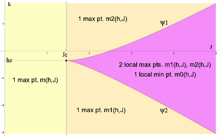
Figure 1: Number and nature of the stationary points of the function $m\mapsto\widetilde{p}\,(m,h,J)$ in the regions of the plane $(h,J)$.

Proof.

Fix $h\in\mathbb{R},\,J>0$ and to shorten the notation set $G(m):=\frac{\partial\widetilde{p}\,}{\partial m}(m,h,J)$, observing it is a continuous (smooth) function.
$\bullet$ Suppose $J\leq J_{c}$. By proposition 3, $G^{\prime}(m)\leq 0$ for all $m\in\mathbb{R}$ and equality holds iff ($J=J_{c}$ and $m=\phi_{1}(h,J_{c})=\phi_{2}(h,J_{c})\,$). Hence $G$ is strictly decreasing on $\mathbb{R}$. On the other hand by (33), $G(m)<0$ for all $m\leq 0$ and $G(m)>0$ for all $m\geq 1$. Therefore there exists a unique point $m$ ($m\in\,]0,1[\,$) such that $G(m)=0$.
$\bullet$ Suppose $J>J_{c}$. By proposition 3, $G$ is strictly decreasing for $m\leq\phi_{1}(h,J)$, strictly increasing for $\phi_{1}(h,J)\leq m\leq\phi_{2}(h,J)$ and again strictly decreasing for $m\geq\phi_{2}(h,J)$. On the other hand by (33), $G(m_{+})>0$ for some point $m_{+}<\phi_{1}(h,J)$ and $G(m_{-})>0$ for some point $m_{-}>\phi_{2}(h,J)$. Therefore:

$$(\,\exists\,(\text{a$\!$ unique})\;m_{1}\in\,]-\infty,\phi_{1}(h,J)]\ \text{s.t.}\ G(m_{1})=0\,)\ \Leftrightarrow\ G(\phi_{1}(h,J))\leq 0\,;$$

$$(\,\exists\,(\text{a$\!$ unique})\;m_{2}\in[\phi_{2}(h,J),\infty[\,\ \text{s.t.}\ G(m_{2})=0\,)\ \Leftrightarrow\ G(\phi_{2}(h,J))\geq 0\,;$$

$$(\,\exists\,(\text{a$\!$ unique})\;m_{0}\in[\phi_{1}(h,J),\phi_{2}(h,J)]\,\ \text{s.t.}\ G(m_{0})=0\,)\ \Leftrightarrow\ G(\phi_{1}(h,J))\leq 0\,,\;G(\phi_{2}(h,J))\geq 0\,.$$

And now, using identity (31) and definitions (38), (40)

$$G(\phi_{1}(h,J))\underset{(=)}{<}0\ \Leftrightarrow\ g\big{(}(2\phi_{1}(h,J)-1)J+h\big{)}\underset{(=)}{<}\phi_{1}(h,J)\ \Leftrightarrow\ h\underset{(=)}{<}\psi_{1}(J)$$

and similarly $G(\phi_{2}(h,J))\underset{(=)}{>}0\ \Leftrightarrow\ h\underset{(=)}{>}\psi_{2}(J)\,$.
The first $\bullet$ allows to conclude in case 1., while the second $\bullet$ allows to conclude in all the other cases. Notice that the nature of the stationary points of $\widetilde{p}\,(\cdot\,,h,J)$ is determined by the sign of the second derivative $\frac{\partial^{2}\widetilde{p}\,}{\partial m^{2}}$ studied in proposition 3. ∎

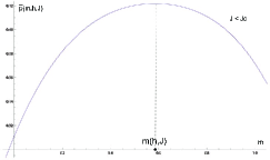
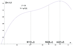
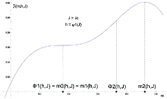
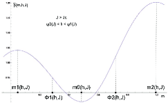
Figure 2: Plots of the function $m\mapsto\widetilde{p}\,(m,h,J)$ for different values of the parameters $h,J$. In particular cases 1., 3., 4., 2. of proposition 4 are represented.

A special role is played by the point $(h_{c},J_{c})$, where we set

$$h_{c}:=\psi_{1}(J_{c})=\psi_{2}(J_{c})\,=\,\frac{1}{2}\,\log(2\sqrt{2}-2)-\frac{1}{4}\,\approx\,-0.3441\;,$$ (41)

indeed in the next sub-sections it will turn out to be the critical point of the system. It is also useful to define

$$m_{c}:=\phi_{1}(h_{c},J_{c})=\phi_{2}(h_{c},J_{c})\,=\,2-\sqrt{2}\,\approx\,0.5857\;,$$ (42)

$$\xi_{c}:=(2m_{c}-1)J_{c}+h_{c}\,=\,\frac{1}{2}\,\log(2\sqrt{2}-2)\,\approx\,-0.0941\;.$$ (43)

The computations are done observing that $a_{1}(J_{c})=a_{2}(J_{c})=2\sqrt{2}-2\,$ and $g(\frac{1}{2}\log(2\sqrt{2}-2))=2-\sqrt{2}$.

Remark 12.

We notice that $m_{c}$ is the (unique) solution of equation (34) for $h=h_{c}$ and $J=J_{c}$, that is $m(h_{c},J_{c})=m_{c}$. Indeed a direct computation using (28) shows

$$\begin{split}g\big{(}(2m_{c}-1)J_{c}+h_{c}\big{)}\,&=\,g\big{(}\xi_{c}\big{)}\,=m_{c}.\\ \end{split}$$

Observe that as a consequence $m_{c}$ is a solution of equation (34) for all $(h,J)$ such that $h-h_{c}=(1-2m_{c})(J-J_{c})$.

In the next proposition we analyse the regularity of the solutions of equation (34).

Proposition 5 (Regularity properties).

Consider the stationary points of $\widetilde{p}\,(\cdot\,,h,J)$ defined in proposition 4: $m(h,J),\,m_{1}(h,J),\,m_{0}(h,J),\,m_{2}(h,J)$ for suitable values of $h,J$. The functions

$$\mu_{1}(h,J):=\,\begin{cases}\,m(h,J)&\text{if }\ 0<J\leq J_{c}\,,\ h\in\mathbb{R}\\ \,m_{1}(h,J)&\text{if }\ J>J_{c}\,,\ h\leq\psi_{1}(J)\end{cases}\;;$$ (44)

$$\mu_{2}(h,J):=\,\begin{cases}\,m(h,J)&\text{if }\ 0<J\leq J_{c}\,,\ h\in\mathbb{R}\\ \,m_{2}(h,J)&\text{if }\ J>J_{c}\,,\ h\geq\psi_{2}(J)\end{cases}\;;$$ (45)

$$\mu_{0}(h,J):=\,\begin{cases}\,m(h,J)&\text{if }\ 0<J\leq J_{c}\,,\ h\in\mathbb{R}\\ \,m_{0}(h,J)&\text{if }\ J>J_{c}\,,\ \psi_{2}(J)\leq h\leq\psi_{1}(J)\end{cases}\;.$$ (46)

have the following properties:

• are continuous on the respective domains;

• are $C^{\infty}$ in the interior of the respective domains;

• for $i=0,1,2$ and $(h,J)$ in the interior of the domain of $\mu_{i}$

  $$\frac{\partial}{\partial h}\,\widetilde{p}\,(\mu_{i}(h,J),h,J)\,=\,\mu_{i}\;,\quad\frac{\partial}{\partial J}\,\widetilde{p}\,(\mu_{i}(h,J),h,J)\,=-\,\mu_{i}\,(1-\mu_{i})\;;$$ (47)

  $$\frac{\partial\mu_{i}}{\partial h}\,=\,\frac{2\,\mu_{i}\,(1-\mu_{i})}{2-\mu_{i}-4J\,\mu_{i}\,(1-\mu_{i})}\;,\qquad\frac{\partial\mu_{i}}{\partial J}\,=\,(2\mu_{i}-1)\,\frac{\partial\mu_{i}}{\partial h}\;.$$ (48)

Proof.

i) First prove the continuity of $\mu_{1}$. Observe that by propositions 4, 3:

• for $(h,J)$ in $D_{1}:=\{(h,J)\,|\,(0<J\leq J_{c},\,h\in\mathbb{R})\;\text{or}\;(J>J_{c},\,h\leq\psi_{2}(J))\}\,$, $\mu_{1}(h,J)$ is the only maximum point of $\widetilde{p}\,(\cdot\,,h,J)$ on the interval $[0,1]\,$;

• for $(h,J)$ in $D_{2}:=\,\{(h,J)\,|\,J\geq J_{c},\,h\leq\psi_{1}(J)\}\,$, $\mu_{1}(h,J)$ is the only maximum point of $\widetilde{p}\,(\cdot\,,h,J)$ on the interval $[0,\phi_{1}(h,J)]\,$.

Hence by proposition B1, continuity of the functions $\widetilde{p}\,$ and $\phi_{1}$ implies continuity of the function $\mu_{1}$ on the sets $D_{1}$ and $D_{2}$. As $D_{1}$ and $D_{2}$ are both closed subsets of $\mathbb{R}\times\mathbb{R}_{+}$, by the pasting lemma $\mu_{1}$ is continuous on their union

$$D_{1}\cup D_{2}\,=\,\{(h,J)\;|\;(0<J\leq J_{c},\,h\in\mathbb{R})\ \text{or}\ (J>J_{c},\,h\leq\psi_{1}(J))\}\;.$$

A similar argument proves the continuity of $\mu_{2}$ and $\mu_{0}$.
ii) Now prove the smoothness of $\mu_{1},\,\mu_{2},\,\mu_{0}$ in the interior of their domains. Set $G(m,h,J):=\frac{\partial\widetilde{p}\,}{\partial m}(m,h,J)$. As just seen $m=\mu_{1}(h,J),\,\mu_{2}(h,J),\,\mu_{0}(h,J)$ are continuous solutions of

$$G(m,h,J)=0\;,$$

for values of $h,J$ in the respective domains. Observe that $G\in C^{\infty}(\mathbb{R}\times\mathbb{R}\times\mathbb{R}_{+})$ and by propositions 3, 4 it can happen

$$\begin{split}&\begin{cases}\dfrac{\partial G}{\partial m}\,(m,h,J)=0\\[2.0pt] G(m,h,J)=0\end{cases}\Leftrightarrow\ \begin{cases}J\geq J_{c}\,,\;(m=\phi_{1}(h,J)\text{ or }m=\phi_{2}(h,J))\\[2.0pt] G(m,h,J)=0\end{cases}\!\!\Leftrightarrow\\[4.0pt] &\Leftrightarrow\ \begin{cases}J\geq J_{c},\,m=\phi_{1}(h,J)\\[2.0pt] h=\psi_{1}(J)\end{cases}\!\!\text{or }\ \begin{cases}J\geq J_{c},\,m=\phi_{2}(h,J)\\[2.0pt] h=\psi_{2}(J)\end{cases}\!\!.\end{split}$$

$m=\mu_{1}(h,J)$ can fall only within the first case, while $m=\mu_{2}(h,J)$ can fall only within the second case. Therefore by the implicit function theorem (corollary B1), $\mu_{1},\,\mu_{2},\,\mu_{0}$ are $C^{\infty}$ on the interior of the respective domains.
iii) Let $i=0,1,2$ and $(h,J)$ in the interior of the domain of $\mu_{i}$. Using (30), $(p^{\textup{\tiny{MD}}})^{\prime}=g$ and the fact that $\mu_{i}(h,J)$ satisfies equation (34), compute

$$\begin{split}\frac{\partial}{\partial h}\,\widetilde{p}\,(\mu_{i},h,J)\,&=-2J\,\frac{\partial\mu_{i}}{\partial h}+(p^{\textup{\tiny{MD}}})^{\prime}\big{(}(2\mu_{i}-1)J+h\big{)}\,(2J\,\frac{\partial\mu_{i}}{\partial h}+1)\\ &=-2J\,\frac{\partial\mu_{i}}{\partial h}+\mu_{i}\,(2J\,\frac{\partial\mu_{i}}{\partial h}+1)\,=\,\mu_{i}\;;\end{split}$$

and similarly $\frac{\partial}{\partial J}\,\widetilde{p}\,(\mu_{i},h,J)=\mu_{i}^{2}-\mu_{i}\,$.
Using the fact that $\mu_{i}(h,J)$ satisfies equation (34) compute

$$\begin{split}&\frac{\partial\mu_{i}}{\partial h}\,=\,\frac{\partial}{\partial h}\,g\big{(}(2\mu_{i}-1)J+h\big{)}\,=\,g^{\prime}\big{(}(2\mu_{i}-1)J+h)\big{)}\,(1+2J\,\frac{\partial\mu_{i}}{\partial h})\\ &\Rightarrow\ \frac{\partial\mu_{i}}{\partial h}\,=\,\frac{g^{\prime}\big{(}(2\mu_{i}-1)J+h\big{)}}{1-2J\,g^{\prime}\big{(}(2\mu_{i}-1)J+h\big{)}}\;;\end{split}$$

and similarly $\frac{\partial\mu_{i}}{\partial J}=\frac{(2\mu_{i}-1)\,g^{\prime}\big{(}(2\mu_{i}-1)J+h\big{)}}{1-2J\,g^{\prime}\big{(}(2\mu_{i}-1)J+h\big{)}}\,$. Then observe that $g^{\prime}=2\,g\,(1-g)/(2-g)$ (identity (A2) in the Appendix), hence since $\mu_{i}(h,J)$ satisfies equation (34)

$$g^{\prime}\big{(}(2\mu_{i}-1)J+h\big{)}\,=\,\frac{2\,\mu_{i}\,(1-\mu_{i})}{2-\mu_{i}}\;;$$

substituting this in the previous identities concludes the proof. ∎

To end this subsection we study the asymptotic behaviour of the stationary points of $\widetilde{p}\,(\cdot\,,h,J)$ for large $J$.

Proposition 6 (Asymptotic behaviour).

Consider the stationary points $m_{1}(h,J)$, $m_{0}(h,J)$, $m_{2}(h,J)$ defined in proposition 4 for suitable values of $h,J$.

• For all fixed $h\in\mathbb{R}$

  $$m_{1}(h,J)\,\xrightarrow[J\to\infty]{}\,0\;,\quad m_{2}(h,J)\,\xrightarrow[J\to\infty]{}\,1\;,\quad m_{0}(h,J)\,\xrightarrow[J\to\infty]{}\,\frac{1}{2}\;.$$

• Moreover for all fixed $h\in\mathbb{R}$

  $$J\,m_{1}(h,J)\,\xrightarrow[J\to\infty]{}\,0\;,\quad J\,(1-m_{2}(h,J))\,\xrightarrow[J\to\infty]{}\,0\;.$$

• And taking the $\sup$ and $\inf$ over $h\in[\psi_{2}(J),\psi_{1}(J)]\,$

  $$\sup_{h}m_{1}(h,J)\,\xrightarrow[J\to\infty]{}\,0\;,\quad\inf_{h}m_{2}(h,J)\,\xrightarrow[J\to\infty]{}\,1\;.$$

Proof.

i) First observe from the definition (40) that $\psi_{2}(J)\rightarrow-\infty$, $\psi_{1}(J)\rightarrow\infty$ as $J\to\infty$. Hence for any fixed $h\in\mathbb{R}$ there exists $\bar{J}>0$ such that $\psi_{2}(J)<h<\psi_{1}(J)$ for all $J>\bar{J}$. This means that the limits in the statement make sense.
Now remind that by proposition 4, for $J>\bar{J}$

$$m_{1}(h,J)<\phi_{1}(h,J)<m_{0}(h,J)<\phi_{2}(h,J)<m_{2}(h,J)\;.$$

Observe from the definition (38) that $\phi_{1}(h,J)\rightarrow\frac{1}{2}\,$, $\phi_{2}(h,J)\rightarrow\frac{1}{2}\,$ as $J\to\infty$. It follows immediately that also $m_{0}(h,J)\rightarrow\frac{1}{2}$ as $J\to\infty$.
Moreover definition (38) entails that $J\big{(}\frac{1}{2}-\phi_{1}(h,J)\big{)}\rightarrow\infty\,$, $J\big{(}\phi_{2}(h,J)-\frac{1}{2}\big{)}\rightarrow\infty$ as $J\to\infty$. Exploit the fact that $m_{1}(h,J)$ is a solution of equation (34):

$$\begin{split}m_{1}(h,J)\,&=\,g\big{(}(2m_{1}(h,J)-1)\,J+h\big{)}\,\leq\,g\big{(}(2\phi_{1}(h,J)-1)\,J+h\big{)}\,=\\ &=\,g\big{(}-2J\,(\frac{1}{2}-\phi_{1}(h,J))+h\big{)}\,\xrightarrow[J\to\infty]{}\,0\;,\end{split}$$

where also the facts that the function $g$ is increasing and $g(\xi)\rightarrow 0$ as $\xi\to-\infty$ are used. As by remark 10 $m_{1}$ takes values in $]0,1[$, conclude that $m_{1}(h,J)\longrightarrow 0$ as $J\to\infty$. Similarly it can be shown that $m_{2}(h,J)\longrightarrow 1$ as $J\to\infty$.
ii) Start observing that, by a standard computation from the definition (28), $\xi\,g(-\xi)\longrightarrow 0$ and $\xi\,\big{(}1-g(\xi)\big{)}\longrightarrow 0$ as $\xi\to+\infty$. Then exploit the fact that, for fixed $h$ and $J$ sufficiently large, $m_{1}=m_{1}(h,J)$ is a solution of equation (34):

$$\begin{split}&J\,m_{1}\,=\,J\,g\big{(}(2m_{1}-1)J+h\big{)}\,=\\[2.0pt] &=\frac{\big{(}(1-2m_{1})J-h\big{)}\;g\big{(}\!-(1-2m_{1})J+h\big{)}}{1-2m_{1}}\,+\frac{h\;g\big{(}\!-(1-2m_{1})J+h\big{)}}{1-2m_{1}}\,\xrightarrow[J\to\infty]{}\,\frac{0}{1}\,+\frac{h\,0}{1}\,=0\,,\end{split}$$

using also that $m_{1}\rightarrow 0$ as $J\to\infty$ by i). Similarly it can be shown that $J\,(1-m_{2})\longrightarrow 0$ as $J\to\infty$.
iii) Start observing that, by a standard computation from the definition (40), $-J+\psi_{1}(J)\longrightarrow-\infty$ and $J+\psi_{2}(J)\longrightarrow\infty$ as $J\to\infty$. Then exploit the fact that, for $J>J_{c}$ and $h\in[\psi_{2}(J),\psi_{1}(J)]$, $m_{1}=m_{1}(h,J)$ is a solution of equation (34):

$$\begin{split}\sup_{h\in[\psi_{2},\psi_{1}]}m_{1}\,&=\,\sup_{h\in[\psi_{2},\psi_{1}]}g\big{(}(2m_{1}-1)J+h\big{)}\,\leq\,g\big{(}(2m_{1}-1)J+\psi_{1}(J)\big{)}\,=\\ &=\,g\big{(}2J\,m_{1}-J+\psi_{1}(J)\big{)}\,\xrightarrow[J\to\infty]{}\,0\;,\end{split}$$

using also the facts that $g$ is an increasing function, $g(\xi)\to 0$ as $\xi\to-\infty$, and $J\,m_{1}\rightarrow 0$ as $J\to\infty$ by ii). Similarly it can be shown that $\inf_{h\in[\psi_{2},\psi_{1}]}m_{2}\longrightarrow 1$ as $J\to\infty$. ∎

IV.2 The “wall”: existence and uniqueness, regularity and asymptotic behavior

In the previous subsection we studied all the solutions of equation (34), that is all the stationary points of $m\mapsto\widetilde{p}\,(m,h,J)$. One of them is the point where the global maximum is attained and, because of theorem 2 and remark 11, we are interested in this one.
Consider the points $m,\,m_{1},\,m_{0},\,m_{2}$ defined in proposition 4 and look for the global maximum point of $m\mapsto\widetilde{p}\,(m,h,J)$:

• for $0<J<J_{c}$ and $h\in\mathbb{R}$, $m(h,J)$ is the only local maximum point, hence it is the global maximum point;

• for $J>J_{c}$ and $h\leq\psi_{2}(J)$, $m_{1}(h,J)$ is the only local maximum point, hence it is the global maximum point;

• for $J>J_{c}$ and $h\geq\psi_{1}(J)$, $m_{2}(h,J)$ is the only local maximum point, hence it is the global maximum point;

• for $J>J_{c}$ and $\psi_{2}(J)<h<\psi_{1}(J)$, there are two local maximum points $m_{1}(h,J)<m_{2}(h,J)$, hence at least one of them is the global maximum point.

To answer which one is the global maximum point in the last case, we have to investigate the sign of the following function

$$\Delta(h,J):=\,\widetilde{p}\,\big{(}m_{2}(h,J),h,J\big{)}-\widetilde{p}\,\big{(}m_{1}(h,J),h,J\big{)}$$ (49)

for $J>J_{c}$ and $\psi_{2}(J)\leq h\leq\psi_{1}(J)\,$.

Proposition 7 (Existence and Uniqueness).

For all $J>J_{c}$ there exists a unique $h=\gamma(J)\in\,]\psi_{2}(J),\psi_{1}(J)[\,$ such that $\Delta(h,J)=0$. Moreover

$$\Delta(h,J)\begin{cases}<0&\text{if }\ J>J_{c},\ \psi_{2}(J)\leq h<\gamma(J)\\[2.0pt] >0&\text{if }\ J>J_{c},\ \gamma(J)<h\leq\psi_{1}(J)\end{cases}\ .$$

Proof.

It is an application of the intermediate value theorem. Fix $J>J_{c}$. It suffices to observe that

• $\Delta\big{(}\psi_{2}(J),J\big{)}<0$, because for $h=\psi_{2}(J)$ the only maximum point of the function $\widetilde{p}\,(\cdot\,,h,J)$ is $m_{1}(h,J)$;

• $\Delta\big{(}\psi_{1}(J),J\big{)}>0$, because for $h=\psi_{1}(J)$ the only maximum point of the function $\widetilde{p}\,(\cdot\,,h,J)$ is $m_{2}(h,J)$;

• $h\mapsto\Delta(h,J)$ is a continuous function, by continuity of $\widetilde{p}\,$, $m_{1}$, $m_{2}$ (see proposition 5);

• $h\mapsto\Delta(h,J)$ is strictly increasing; indeed it is $C^{\infty}$ on $\,]\psi_{2}(J),\psi_{1}(J)[\,$ by smoothness of $\widetilde{p}\,$, $m_{1}$, $m_{2}$ (see proposition 5) and, by formula (47),

  $$\begin{split}\frac{\partial\Delta}{\partial h}\,(h,J)\,&=\,\frac{\partial}{\partial h}\,\widetilde{p}\,\big{(}m_{2}(h,J),h,J\big{)}-\frac{\partial}{\partial h}\,\widetilde{p}\,\big{(}m_{1}(h,J),h,J\big{)}\,=\\ &=\,m_{2}(h,J)-m_{1}(h,J)\,>\,\phi_{2}(h,J)-\phi_{1}(h,J)\,>\,0\end{split}$$

  for all $h\in\,]\psi_{2}(J),\psi_{1}(J)[\,$.∎

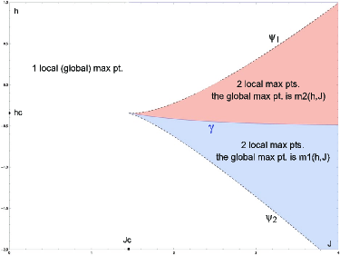
Figure 3: $\gamma$ separates the values of $h,J$ for which $m_{1}(h,J)$ is the global maximum point from those for which $m_{2}(h,J)$ is the global maximum point of $m\mapsto\widetilde{p}\,(m,h,J)$. As $m_{1}(h,J)<m_{2}(h,J)$, this entails a discontinuity of the global maximum point $m^{*}(h,J)$ along the “wall” $\Gamma$.

Remark 13.

By the previous results the global maximum point of $m\mapsto\widetilde{p}\,(m,h,J)$ is

$$m^{*}(h,J):=\begin{cases}\,m(h,J)&\text{if }\;0<J\leq J_{c}\,,\ h\in\mathbb{R}\\ \,m_{1}(h,J)&\text{if }\;J>J_{c}\,,\ h<\gamma(J)\\ \,m_{2}(h,J)&\text{if }\;J>J_{c}\,,\ h>\gamma(J)\end{cases}$$ (50)

where the function $\gamma$ is defined by proposition 7. Set also

$$\Gamma:=\{(h,J)\;|\;J>J_{c},\;h=\gamma(J)\}\;,\qquad\overline{\Gamma}:=\,\Gamma\,\cup\,\{(h_{c},J_{c})\}\ .$$ (51)

Notice that proposition 7 guarantees that there is only a curve $\Gamma$ in the plane $(h,J)$ where the global maximum point of $m\mapsto\widetilde{p}\,(m,h,J)$ is not unique. We leaved the function $m^{*}$ undefined on $\Gamma$.
By proposition 5 it follows that the function $m^{*}$ is continuous on its domain $(\mathbb{R}\times\mathbb{R}_{+})\smallsetminus\Gamma$ and it is $C^{\infty}$ on $(\mathbb{R}\times\mathbb{R}_{+})\smallsetminus\overline{\Gamma}\,$. The behaviour of $m^{*}$ at the critical point $(h_{c},J_{c})$ will be investigated in the next subsection.

Now we investigate the main properties of the curve $\overline{\Gamma}$, which we call “the wall”. Extend the function $\gamma$ defined by proposition 7 by

$$\overline{\gamma}(J):=\begin{cases}\,\gamma(J)&\text{if }\;J>J_{c}\\ \,h_{c}&\text{if }\;J=J_{c}\end{cases}\ .$$ (52)

Proposition 8 (Regularity properties).

The function $\overline{\gamma}$ is $C^{\infty}$ on $]J_{c},\infty[\,$ and (at least) $C^{1}$ on $[J_{c},\infty[$. In particular

$$\gamma^{\prime}(J)\,=\,1-m_{1}\big{(}\gamma(J),J\big{)}-m_{2}\big{(}\gamma(J),J\big{)}\quad\forall\,J>J_{c}\;,$$

and

$$\overline{\gamma}\,^{\prime}(J_{c})\,=\,1-2\,m_{c}\,=\,-(3-2\sqrt{2})\;.$$

Proof.

I. First prove that the function $\gamma\in C^{\infty}(\,]J_{c},\infty[\,)$.
By proposition 7 for all $J>J_{c}$, $h=\gamma(J)$ is the unique solution of equation

$$\Delta(h,J)=0$$

where $\Delta$ is defined by (49). Moreover $\psi_{2}(J)<\gamma(J)<\psi_{1}(J)$. Observe that $\Delta$ is $C^{\infty}$ on $\{(h,J)\,|\,J>J_{c},\;\psi_{2}(J)<h<\psi_{1}(J)\}$ by smoothness of $\widetilde{p}\,$ and $m_{1}$, $m_{2}$ on this region (see proposition 5). And furthermore, as shown in the proof of proposition 7,

$$\frac{\partial\Delta}{\partial h}\,(h,J)\neq 0\quad\forall\,(h,J)\text{ s.t. }h=\gamma(J)\,.$$

Therefore by the implicit function theorem (corollary B2), $\gamma\in C^{\infty}(\,]J_{c},\infty[\,)$. Now

$$\begin{split}&\Delta(\gamma(J),J))\equiv 0\ \Rightarrow\ 0=\frac{\mathrm{d}}{\mathrm{d}J}\,\Delta(\gamma(J),J)=\frac{\partial\Delta}{\partial h}(\gamma(J),J)\,\gamma^{\prime}(J)+\frac{\partial\Delta}{\partial J}(\gamma(J),J)\\ &\Rightarrow\ \gamma^{\prime}(J)\,=-\,\frac{\partial\Delta}{\partial J}\,\big{/}\,\frac{\partial\Delta}{\partial h}\;(\gamma(J),J)\;;\end{split}$$

by formulae (47) $\frac{\partial\Delta}{\partial h}=m_{2}-m_{1}$ and $\frac{\partial\Delta}{\partial J}=(m_{2}^{2}-m_{2})-(m_{1}^{2}-m_{1})\,$; therefore

$$\begin{split}\gamma^{\prime}(J)\,&=\,1-(m_{2}+m_{1})\,(\gamma(J),J)\;.\end{split}$$

II. Now prove that the extended function $\overline{\gamma}\in C^{1}([J_{c},\infty[)\,$.
First observe that $\overline{\gamma}$ is continuous also in $J_{c}$, indeed:

$$\psi_{2}(J)<\gamma(J)<\psi_{1}(J)\ \ \forall\,J>J_{c}\quad\Rightarrow\quad\lim_{J\to J_{c}+}\gamma(J)=h_{c}$$

by definition of $h_{c}$ (41) and continuity of $\psi_{1},\,\psi_{2}$. Then observe that

$$\gamma^{\prime}(J)\,=\,1-(m_{2}+m_{1})\,(\gamma(J),J)\ \xrightarrow[J\to J_{c}+]{}\ 1-2m_{c}$$

because $m(h_{c},J_{c})=m_{c}$ (remark 12) and the functions $\mu_{1},\,\mu_{2}$ defined in proposition 5 are continuous. By an immediate application of the mean value theorem, this proves that there exists $\overline{\gamma}\,^{\prime}(J_{c})=1-2m_{c}$. ∎

Proposition 9 (Asymptotic behavior).

The function $\overline{\gamma}$ has an asymptote, precisely

$$\gamma(J)\,\xrightarrow[J\to\infty]{}\,-\frac{1}{2}\;.$$

Proof.

I. Consider the function $\Delta$ defined by (49). The first step is to prove that $\Delta(h,J)\longrightarrow 0$ as $J\to\infty$, $h=-\frac{1}{2}\,$. Use identities (30), (27) and the fact that for fixed $h$ and $J$ sufficiently large $m_{1}=m_{1}(h,J)$, $m_{2}=m_{2}(h,J)$ satisfy equation (34), in two different ways:

$$\widetilde{p}\,(m_{1},h,J)\,=\,-J\,m_{1}^{2}+\frac{J}{2}-\frac{1-m_{1}}{2}-\log g\big{(}(2m_{1}-1)J+h\big{)}+(2m_{1}-1)J+h\;,$$

$$\widetilde{p}\,(m_{2},h,J)\,=\,-J\,m_{2}^{2}+\frac{J}{2}-\frac{1-m_{2}}{2}-\log m_{2}+(2m_{2}-1)J+h\;.$$

Hence, reminding that $m_{1}\rightarrow 0$ and $m_{2}\rightarrow 1$ as $J\to\infty$ by proposition 6 part i),

$$\begin{split}\Delta(h,J)\,&=\,\widetilde{p}\,(m_{2},h,J)-\widetilde{p}\,(m_{1},h,J)\,=\\ &=\,J\,(-m_{2}^{2}+2m_{2}+m_{1}^{2}-2m_{1})+\log g\big{(}(2m_{1}-1)J+h\big{)}+\frac{1}{2}+o(1)\;,\end{split}$$

Set $\delta:=-m_{2}^{2}+2m_{2}+m_{1}^{2}-2m_{1}$ and $\xi:=(2m_{1}-1)J+h$ and prove that in general

$$J\,\delta+\log g(\xi)\,\xrightarrow[J\to\infty]{}\,h\;;$$ (53)

in particular it will follow that for $h=-\frac{1}{2}$

$$\Delta\big{(}-\frac{1}{2},\,J\big{)}\,\xrightarrow[J\to\infty]{}\,0\;.$$ (54)

Now proving (53) is equivalent to prove $\exp(J\delta)\,g(\xi)\longrightarrow\exp(h)$ as $J\to\infty$; and using definition (28)

$$e^{J\delta}\,g(\xi)\,=\,e^{J\delta}\,\frac{\sqrt{e^{4\xi}+4e^{2\xi}}-e^{2\xi}}{2}\;=\,\frac{\sqrt{e^{2(J\delta+2\xi)}+4e^{2(J\delta+\xi)}}-e^{J\delta+2\xi}}{2}\,\xrightarrow[J\to\infty]{}\,e^{h}\;,$$

because, since $J\,m_{1}\rightarrow 0$ and $J\,(1-m_{2})\rightarrow 0$ as $J\to\infty$ by proposition 6 part ii),

$$J\delta+2\xi\,=\,J\,\big{(}\!-(1-m_{2})^{2}+m_{1}^{2}-2m_{1}-1\,\big{)}+2h\;\xrightarrow[J\to\infty]{}\,-\infty\;,$$

$$J\delta+\xi\,=\,J\,\big{(}\!-(1-m_{2})^{2}+m_{1}^{2}\,\big{)}+h\;\xrightarrow[J\to\infty]{}\;h\;.$$

II. Remember that by definition of $\gamma$ in proposition 7

$$\Delta\big{(}\gamma(J),J\big{)}\,=\,0\quad\forall\,J>J_{c}\;;$$ (55)

hence using (54) will not be hard to prove that $\gamma(J)\longrightarrow-\frac{1}{2}$ as $J\to\infty$. Let $\epsilon>0$. By (54) there exists $\bar{J}_{\epsilon}>J_{c}$ such that

$$\big{|}\Delta\big{(}\!-\frac{1}{2},\,J\big{)}\big{|}<\,\epsilon\quad\forall\,J>\bar{J}_{\epsilon}\;.$$ (56)

Now by the mean value theorem for all $J>J_{c}$ and $h\in[\psi_{2}(J),\psi_{1}(J)]$,

$$\big{|}\Delta(h,J)-\Delta\big{(}\!-\frac{1}{2},\,J\big{)}\big{|}\;\geq\;\inf_{[\psi_{2}(J),\psi_{1}(J)]}\big{|}\frac{\partial\Delta}{\partial h}\,(\cdot\,,J)\big{|}\;\big{|}h+\frac{1}{2}\,\big{|}\;.$$

Furthermore by identity (47) and proposition 6 part iii)

$$\begin{split}&\inf_{[\psi_{2}(J),\psi_{1}(J)]}\big{|}\frac{\partial\Delta}{\partial h}\,(\cdot\,,J)\big{|}\;=\,\inf_{[\psi_{2}(J),\psi_{1}(J)]}(m_{2}-m_{1})\,(\cdot\,,J)\,\geq\\[2.0pt] &\geq\,\inf_{[\psi_{2}(J),\psi_{1}(J)]}m_{2}(\cdot,J)\;-\sup_{[\psi_{2}(J),\psi_{1}(J)]}m_{1}\,(\cdot,J)\;\xrightarrow[J\to\infty]{}\;1\;.\end{split}$$

Therefore there exist $\bar{J}$ such that

$$\big{|}\Delta(h,J)-\Delta\big{(}\!-\frac{1}{2},\,J\big{)}\big{|}\;\geq\;\frac{1}{2}\ \big{|}h+\frac{1}{2}\,\big{|}\quad\ \forall\,J\!>\bar{J},\,h\!\in[\psi_{2}(J),\psi_{1}(J)]\,.$$ (57)

Choosing $h=\gamma(J)$ in (57), by (55), (56) one obtains that for all $J>\max\{\bar{J},\,\bar{J}_{\epsilon}\}$

$$\big{|}\gamma(J)+\frac{1}{2}\,\big{|}\,\leq\;2\,\big{|}\Delta(\gamma(J),J)-\Delta\big{(}\!-\frac{1}{2},J\big{)}\big{|}<\,2\epsilon\;.\qed$$

IV.3 Critical exponents

As observed in remark 13 the global maximum point $m^{*}(h,J)$ is a continuous function on $(\mathbb{R}\times\mathbb{R}^{+})\smallsetminus\Gamma$, but it is smooth only outside the critical point $(h_{c},J_{c})$. In this section we study the behaviour of the solutions of equation (34) near the critical point, with particular interest in the function $m^{*}$.

As usual the notation $f=\mathcal{O}(g)$ as $x\to x_{0}$ means that there exists a neighbourhood $U$ of $x_{0}$ and a constant $C\in\mathbb{R}$ such that $|f(x)|\leq C\,|g(x)|$ for all $x\in U$. The notation $f\sim g$ as $x\to x_{0}$ means that $f(x)/g(x)\longrightarrow 1$ as $x\to x_{0}$. Finally $f=o(g)$ as $x\to x_{0}$ means that $f(x)/g(x)\longrightarrow 0$ as $x\to x_{0}$.

We call critical exponent of a function $f$ at a point $x_{0}$ the following limit

$$\lim_{x\to x_{0}}\frac{\log|f(x)-f(x_{0})|}{\log|x-x_{0}|}\;.$$

The main result of this section is the following:

Theorem 3.

Consider the global maximum point $m^{*}(h,J)$ of the function $m\mapsto\widetilde{p}\,(m,h,J)$ defined by (30).

• $m^{*}$ is continuous on $(\mathbb{R}\times\mathbb{R}_{+})\smallsetminus\Gamma$ and smooth on $(\mathbb{R}\times\mathbb{R}_{+})\smallsetminus\overline{\Gamma}$, where $\overline{\Gamma}=\Gamma\cup\{(h_{c},J_{c})\}$ and the “wall” curve $\Gamma$ is the graph of the function $\gamma$ defined by proposition 7.

• The critical exponents of $m^{*}$ at the critical point $(h_{c},J_{c})$ are:

  $$\boldsymbol{\beta}\,=\lim_{J\to J_{c}+}\frac{\log|m^{*}(\delta(J),J)-m_{c}|}{\log(J-J_{c})}\;=\,\frac{1}{2}$$

  along any curve $h=\delta(J)$ with $\delta\in C^{2}([J_{c},\infty[)$, $\delta(J_{c})=h_{c}$, $\delta^{\prime}(J_{c})=1-2m_{c}$ (i.e. if the curve is tangent to the “wall” in the critical point);

  $$\frac{1}{\boldsymbol{\delta}}\,=\lim_{J\to J_{c}}\frac{\log|m^{*}(\delta(J),J)-m_{c}|}{\log|J-J_{c}|}\;=\,\frac{1}{3}$$

  $$\frac{1}{\boldsymbol{\delta}}\,=\lim_{h\to h_{c}}\frac{\log|m^{*}(h,\delta(h))-m_{c}|}{\log|h-h_{c}|}\;=\,\frac{1}{3}$$

  along any curve $h=\delta(J)$ with $\delta\in C^{2}(\mathbb{R}_{+})$, $\delta(J_{c})=h_{c}$, $\delta^{\prime}(J_{c})\neq 1-2m_{c}$ or along a curve $J=\delta(h)$ with $\delta\in C^{2}(\mathbb{R})$, $\delta(h_{c})=J_{c}$, $\delta^{\prime}(h_{c})=0$ (i.e. if the curve is not tangent to the “wall” in the critical point).

• Denote by $m^{*}(h^{\pm},J):=\lim_{h^{\prime}\to h\pm}m^{*}(h^{\prime},J)$. The critical exponent of $m^{*}(h^{+},J)$ and $m^{*}(h^{-},J)$ at the critical point $(h_{c},J_{c})$ along the “wall” $h=\gamma(J)$ is still

  $$\boldsymbol{\beta}\,=\lim_{J\to J_{c}+}\frac{\log|m^{*}(\gamma(J)^{+},J)-m_{c}|}{\log(J-J_{c})}\;=\,\frac{1}{2}$$

  $$\boldsymbol{\beta}\,=\lim_{J\to J_{c}+}\frac{\log|m^{*}(\gamma(J)^{-},J)-m_{c}|}{\log(J-J_{c})}\;=\,\frac{1}{2}$$

Proof.

As observed in remark 13, the global maximum point $m^{*}$ is expressed piecewise using the two local maximum points $\mu_{1}$, $\mu_{2}$ and inherits their continuity property outside $\Gamma$ and their regularity properties outside $\overline{\Gamma}$. Thus part i) of the theorem is already proved by proposition 5.
The proof of the other parts of the theorem, regarding the behaviour of $m^{*}$ at the critical point $(h_{c},J_{c})$, is given in several steps. We start with the following lemma which will be useful in the whole subsection to bound the behaviour of the solutions of equation (34).

Lemma 1.

Consider the inflection points $\phi_{1},\,\phi_{2}$ of $\widetilde{p}\,$ defined by (38). Their behaviour at the critical point $(h_{c},J_{c})$ along any curve $\delta\in C^{1}([J_{c},\infty[)$, with $\delta(J_{c})=h_{c}$, is

$$\frac{\phi_{1}(\delta(J),J)-m_{c}}{\sqrt{J-Jc}}\;\xrightarrow[J\to J_{c}+]{}\,-C\;,\quad\frac{\phi_{2}(\delta(J),J)-m_{c}}{\sqrt{J-Jc}}\;\xrightarrow[J\to J_{c}+]{}\;C\;.$$

where $C=\sqrt[4]{2}/(2J_{c})>0$.

Proof.

For $i=1,2$ and $J\geq J_{c}$ definition (38), observing that $(2m_{c}-1)J=-h_{c}+(2m_{c}-1)\,(J-J_{c})+\xi_{c}\,$, gives

$$2J\,\big{(}\phi_{i}(\delta(J),J)-m_{c}\big{)}\,=\,\frac{1}{2}\log a_{i}(J)-\xi_{c}-(\delta(J)-h_{c})-(2m_{c}-1)(J-J_{c})\;.$$

Now the definition (39) may be rewritten as

$$a_{i}(J)\,=\,\underbrace{(2J-2-\frac{1}{8J})}_{=:\,b(J)}\;\mp\;\underbrace{4\,(\frac{1}{2}-\frac{1}{8J})\,\sqrt{J-\tfrac{3-2\sqrt{2}}{4}}}_{=:\,c(J)}\ \sqrt{J-Jc}\;.$$

Thus, exploiting $\log(x+y)=\log x+\log(1+y/x)=\log x+y/x+\mathcal{O}((y/x)^{2})$ as $y/x\to 0$, $\frac{1}{2}\,\log b(J_{c})=\xi_{c}$ and $\log b(J)$ differentiable at $J=J_{c}$,

$$\begin{split}\frac{1}{2}\log a_{i}(J)-\xi_{c}\,&=\,\frac{1}{2}\,\frac{\log b(J)-\log b(J_{c})}{(J-J_{c})}\;(J-J_{c})\,\mp\,\frac{1}{2}\,\frac{c(J)}{b(J)}\;\sqrt{J-Jc}\,+\mathcal{O}(J-J_{c})\\ &=\,\mp\,\frac{1}{2}\,\frac{c(J)}{b(J)}\;\sqrt{J-J_{c}}\,+\mathcal{O}(J-J_{c})\;.\end{split}$$

To conclude put things together and use also $\delta$ differentiable at $J_{c}$:

$$\begin{split}2J\,\frac{\phi_{i}(\delta(J),J)-m_{c}}{\sqrt{J-Jc}}\,&=\,\frac{\frac{1}{2}\,\log a_{i}(J)-\xi_{c}}{\sqrt{J-J_{c}}}\,-\frac{\delta(J)-h_{c}}{\sqrt{J-J_{c}}}\,-(2m_{c}-1)\sqrt{J-J_{c}}\\[2.0pt] &=\,\mp\frac{1}{2}\,\frac{c(J)}{b(J)}+\mathcal{O}(\sqrt{J-J_{c}}\;)\,\xrightarrow[J\to J_{c}+]{}\;\pm\sqrt[4]{2}\;.\qed\end{split}$$

In the following proposition we find the fundamental equation characterizing the behaviour of the solutions of equation (34) near the critical point $(h_{c},J_{c})$.

Proposition 10.

Here for $h\in\mathbb{R},\,J>0$ let $m=m(h,J)$ be any solution of the consistency equation (34):

$$m=g\big{(}(2m-1)J+h\big{)}\;.$$

Then $m$ is continuous at $(h_{c},J_{c})$ and furthermore, setting $\xi:=(2m-1)J+h$, it satisfies

$$(\xi-\xi_{c})^{3}-\kappa_{1}\,(J-J_{c})\,(\xi-\xi_{c})-\kappa_{2}\,\rho(h,J)+\mathcal{O}\big{(}(\xi-\xi_{c})^{4}\big{)}=0$$ (58)

as $(h,J)\to(h_{c},J_{c})$, where we set $\kappa_{1}:=3\,\frac{J_{c}}{J}\,(2-m_{c})$, $\kappa_{2}:=3\,\frac{J_{c}^{2}}{J}\,(2-m_{c})$ and

$$\rho(h,J):=h-h_{c}+(2m_{c}-1)(J-J_{c})\;.$$ (59)

Proof.

I. First show that $m$ is continuous at $(h_{c},J_{c})$. Exploit equation (34) for $m(h,J)$ and use continuity and monotonicity of $g$: as $(h,J)\to(h_{c},J_{c})$

$$\limsup m(h,J)=\limsup g\big{(}(2\,m(h,J)-1)\,J+h\big{)}=g\big{(}(2\limsup m(h,J)-1)\,J_{c}+h_{c}\big{)}\;,$$

$$\liminf m(h,J)=\liminf g\big{(}(2\,m(h,J)-1)\,J+h\big{)}=g\big{(}(2\liminf m(h,J)-1)\,J_{c}+h_{c}\big{)}\;.$$

Thus $\limsup m(h,J)$ and $\liminf m(h,J)$ are both solution of equation $\mu=g\big{(}(2\mu+1)J_{c}+h_{c}\big{)}$. But this solution is unique by proposition 4, and it is $m_{c}$ by remark 12. Therefore

$$\limsup_{(h,J)\to(h_{c},J_{c})}m(h,J)\,=\liminf_{(h,J)\to(h_{c},J_{c})}m(h,J)\,=\,m_{c}\;.$$

II. Make a Taylor expansion of the smooth function $g$ at the point $\xi_{c}$ (see (28), (43)). By identities (A2), (A3), (A4) and since $g(\xi_{c})=m_{c}$ it is easy to find

$$g(\xi)\,=\,m_{c}+\frac{1}{2J_{c}}\,(\xi-\xi_{c})-\frac{1}{6J_{c}^{2}(2-m_{c})}\,(\xi-\xi_{c})^{3}+\mathcal{O}\big{(}(\xi-\xi_{c})^{4}\big{)}$$ (60)

as $\xi\to\xi_{c}$. Now choose $\xi:=(2m-1)J+h$. Then $g(\xi)=m$ and

$$\xi-\xi_{c}\,=\,\rho(h,J)+2J\,(m-m_{c})\;,$$ (61)

where $\rho(h,J):=h-h_{c}+(2m_{c}-1)(J-J_{c})$. Now (58) follows from (60). ∎

Hereafter we will exploit equation (58) and lemma 1 in order to obtain results on the behaviour near the critical point. Next corollary gives a first bound for the critical exponents.

Corollary 1.

Here for $h\in\mathbb{R},\,J>J_{c}$ let $m=m(h,J)$ be any solution of the consistency equation (34).
1) There exist $r_{1}>0,\,C_{1}<\infty$ such that for all $(h,J)\in B\big{(}(h_{c},J_{c}),r_{1}\big{)}$ with $J>J_{c}$

$$|m-m_{c}|\,\leq\,C_{1}\big{(}\,|h-h_{c}|^{\frac{1}{3}}+|J-J_{c}|^{\frac{1}{3}}\big{)}\;.$$

2) Assume that $m$ pointwise coincides with one of the local maximum points $m_{1}$, $m_{2}$ (see proposition 4). There exist $r_{2}>0,\,C_{2}>0$ such that for all $(h,J)\in B\big{(}(h_{c},J_{c}),r_{2}\big{)}$ with $J>J_{c}$ and $h=\delta(J)$ for some $\delta\in C^{1}([J_{c},\infty[),\,\delta(J_{c})=h_{c}$

$$|m-m_{c}|\,\geq\,C_{2}\,|J-J_{c}|^{\frac{1}{2}}\;.$$

Proof.

1) Set $\xi:=(2m-1)J+h$. By proposition 10, $\xi$ satisfies equation (58), which can be treated as a third degree algebraic equation in $\xi-\xi_{c}$:

$$(\xi-\xi_{c})^{3}\underbrace{-\kappa_{1}\,(J-J_{c})}_{=:\,p}\,(\xi-\xi_{c})\underbrace{-\kappa_{2}\,\rho(h,J)+\mathcal{O}\big{(}(\xi-\xi_{c})^{4}\big{)}}_{=:\,q}=0\;.$$

Analyse the real solutions of this equation. Set $\Delta:=(\frac{q}{2})^{2}+(\frac{p}{3})^{3}$ and observe that $(\frac{q}{2})^{2}>0$ while $(\frac{p}{3})^{3}<0$ as we are assuming $J>J_{c}$.
i. If $\Delta>0$, the only real solution of (58) is

$$\xi-\xi_{c}=u_{+}+u_{-}\quad\text{with }\,u_{\pm}=\sqrt[3]{-\frac{q}{2}\pm\sqrt[2]{\Delta}}\;.$$

On the other hand

$$\Delta>0\ \Rightarrow\ \big{(}\frac{p}{3}\,\big{)}^{3}=\mathcal{O}\big{(}\big{(}\frac{q}{2}\,\big{)}^{2}\big{)}\ \Rightarrow\ \Delta=\mathcal{O}\big{(}\big{(}\frac{q}{2}\,\big{)}^{2}\big{)}\;.$$

Therefore, reminding also definition (59),

$$\xi-\xi_{c}\,=\,\mathcal{O}\big{(}\big{(}\frac{q}{2}\,\big{)}^{\frac{1}{3}}\big{)}\,=\,\mathcal{O}\big{(}(h-h_{c})^{\frac{1}{3}}\big{)}+\mathcal{O}\big{(}(J-J_{c})^{\frac{1}{3}}\big{)}+\mathcal{O}\big{(}(\xi-\xi_{c})^{\frac{4}{3}}\big{)}\;,$$

hence $\xi-\xi_{c}=\mathcal{O}\big{(}(h-h_{c})^{\frac{1}{3}}\big{)}+\mathcal{O}\big{(}(J-J_{c})^{\frac{1}{3}}\big{)}$ because $(\xi-\xi_{c})^{\frac{4}{3}-1}\rightarrow 0$ as $(h,J)\to(h_{c},J_{c})\,$.
ii. If $\Delta=0$ or $\Delta<0$ there are respectively two or three distinct real solutions of (58) and, from their explicit form, it is immediate to see that they all satisfy

$$\xi-\xi_{c}\,=\,\mathcal{O}\big{(}\sqrt[2]{-\frac{p}{3}}\;\big{)}\,=\,\mathcal{O}\big{(}(J-J_{c})^{\frac{1}{2}}\big{)}\;.$$

Conclude that for any possible value of $\Delta$,

$$\xi-\xi_{c}=\mathcal{O}\big{(}(h-h_{c})^{\frac{1}{3}}\big{)}+\mathcal{O}\big{(}(J-J_{c})^{\frac{1}{3}}\big{)}\;.$$

Now, as observed in (61), $\xi-\xi_{c}=h-h_{c}+(2m_{c}-1)(J-J_{c})+2J\,(m-m_{c})$. Therefore also $m-m_{c}=\mathcal{O}\big{(}(h-h_{c})^{\frac{1}{3}}\big{)}+\mathcal{O}\big{(}(J-J_{c})^{\frac{1}{3}}\big{)}\,$, and this concludes the proof of the first statement.
2) Now consider the two maximum points $m_{1},\,m_{2}$. By proposition 4

$$m_{1}<\phi_{1}<\phi_{2}<m_{2}$$

where $\phi_{1},\,\phi_{2}$ are the inflection points defined by (38). Hence applying lemma 1 one finds:

$$\frac{m_{2}-m_{c}}{\sqrt{J-J_{c}}}\,>\,\frac{\phi_{2}-m_{c}}{\sqrt{J-J_{c}}}\,\longrightarrow\;C\,,\quad\frac{m_{c}-m_{1}}{\sqrt{J-J_{c}}}\,>\,\frac{m_{c}-\phi_{1}}{\sqrt{J-J_{c}}}\,\longrightarrow\;C\,,$$

as $J\to J_{c}+$ and $h=\delta(J)$ with $\delta(J_{c})=h_{c}$ and $\delta$ differentiable in $J_{c}$. And this proves the second statement. ∎

The next lemma tells us in which region of the plane $(h,J)$ described by figure 1 a curve passing through the point $(h_{c},J_{c})$ lies.

Lemma 2.

Let $\delta\in C^{2}([J_{c},\infty[)$ such that $\delta(J_{c})=h_{c}$, $\delta^{\prime}(J_{c})=:\alpha$. There exists $r>0$ such that for all $J\in\,]J_{c},J_{c}+r[$

• if $\alpha=1-2m_{c}$, $\;\psi_{2}(J)<\delta(J)<\psi_{1}(J)\,$;

• if $\alpha<1-2m_{c}$, $\;\delta(J)<\psi_{2}(J)\,$;

• if $\alpha>1-2m_{c}$, $\;\delta(J)>\psi_{1}(J)\,$.

Proof.

I. Observe that $a_{i}(J)$ is continuous for $J\geq J_{c}$ and smooth for $J>J_{c}$. Moreover $g^{\prime}(\frac{1}{2}\log a_{i}(J))=\frac{1}{2J}$ by definition (39) and lemma A1, and $g(\frac{1}{2}\log a_{i}(J_{c}))=g(\xi_{c})=m_{c}$ by definition (43) and remark 12. Then differentiating definition (40) at $J>J_{c}$,

$$\psi_{i}^{\prime}(J)\,=\,1-2\,g(\frac{1}{2}\log a_{i}(J))+\frac{1}{2}\,\frac{a_{i}^{\prime}(J)}{a_{i}(J)}\,\big{(}\underbrace{1-2J\,g^{\prime}(\frac{1}{2}\log a_{i}(J))}_{=\,0}\big{)}\,\xrightarrow[J\to J_{c}]{}\,1-2m_{c}\;.\\$$

Hence an immediate application of the mean value theorem shows that for $i=1,2$ there exits $\psi_{i}^{\prime}(J_{c})=1-2m_{c}\,$.
II. Differentiating definition (39) at $J>J_{c}$ shows that $a_{1}^{\prime}(J)\rightarrow-\infty$, $a_{2}^{\prime}(J)\rightarrow+\infty$ as $J\to J_{c}+$, while $a_{i}(J)\rightarrow 2\sqrt{2}-2$ as $J\to J_{c}$. Hence

$$\psi_{i}^{\prime\prime}(J)\,=\,-\,g^{\prime}(\frac{1}{2}\log a_{i}(J))\,\frac{a_{i}^{\prime}(J)}{a_{i}(J)}\,=\,-\frac{1}{2J}\,\frac{a_{i}^{\prime}(J)}{a_{i}(J)}\;\xrightarrow[J\to J_{c}+]{}\;\begin{cases}+\infty&\text{for }i=1\\ -\infty&\text{for }i=2\end{cases}\;.$$

The result is provided comparing the first order Taylor expansions at $J_{c}$ with Lagrange remainder of $\psi_{1}$, $\psi_{2}$ and $\delta$. ∎

The next proposition describes the behaviour near $(h_{c},J_{c})$ of the two local maximum points $\mu_{1},\,\mu_{2}$ defined in proposition 5. The proof of part ii) of the theorem 3 follows immediately.

Proposition 11.

Let $(h,J)\to(h_{c},J_{c})$ along a curve $h=\delta(J)$ with $\delta\in C^{2}(\mathbb{R}_{+})$, $\delta(J_{c})=h_{c}$, $\delta^{\prime}(J_{c})=:\alpha$ or along a curve $J=\delta(h)$ with $\delta\in C^{2}(\mathbb{R})$, $\delta(h_{c})=J_{c}$, $\delta^{\prime}(h_{c})=0$, then

$$\mu_{1}(h,J)-m_{c}\,\sim\,\begin{cases}\,-\,C\,(J-J_{c})^{\frac{1}{2}}&\text{if }h=\delta(J),\,\alpha=1-2m_{c}\text{ and }J>J_{c}\\[2.0pt] \,C_{\alpha}\,(J-J_{c})^{\frac{1}{3}}&\text{if }h=\delta(J),\,\alpha<1-2m_{c}\\[2.0pt] \,C_{\infty}\,(h-h_{c})^{\frac{1}{3}}&\text{if }J=\delta(h)\end{cases}$$

$$\mu_{2}(h,J)-m_{c}\,\sim\,\begin{cases}\,C\,(J-J_{c})^{\frac{1}{2}}&\text{if }h=\delta(J),\,\alpha=1-2m_{c}\text{ and }J>J_{c}\\[2.0pt] \,C_{\alpha}\,(J-J_{c})^{\frac{1}{3}}&\text{if }h=\delta(J),\,\alpha>1-2m_{c}\\[2.0pt] \,C_{\infty}\,(h-h_{c})^{\frac{1}{3}}&\text{if }J=\delta(h)\end{cases}$$

where $C=\frac{1}{2J_{c}}\,\sqrt{3(2-m_{c})}\,$, $C_{\alpha}=\frac{1}{2J_{c}}\,\sqrt[3]{\frac{3}{2}J_{c}(2-m_{c})(2m_{c}-1+\alpha)}\,$, $C_{\infty}=\frac{1}{2J_{c}}\,\sqrt[3]{3J_{c}(2-m_{c})}\,$. To complete the cases, along the line $h=h_{c}+(1-2m_{c})(J-J_{c})$, when $J\leq J_{c}$

$$\mu_{1}(h,J)=\mu_{2}(h,J)=m_{c}.$$

Proof.

Fix $(h,J)$ on the curve given by the graph of $\delta$ and in the rest of the proof denote by $m$ a solution of the consistency equation (34), i.e. $m=g\big{(}(2m-1)J+h\big{)}$. Furthermore when necessary $m$ is assumed to be a local maximum point of $\widetilde{p}\,$. Set $\xi:=(2m-1)J+h$. By proposition 10, $\xi-\xi_{c}\rightarrow 0$ as $(h,J)\to(h_{c},J_{c})$ and it satisfies (58). Solve this equation in the different cases.
i) Suppose $h=\delta(J)$ with $\alpha=1-2m_{c}$. Hence $h-h_{c}=(1-2m_{c})(J-J_{c})+\mathcal{O}\big{(}(J-J_{c})^{2}\big{)}$. Observe that by (59), (61)

$$\rho(h,J)=\mathcal{O}\big{(}(J-J_{c})^{2}\big{)}\quad\text{and}\quad\xi-\xi_{c}=2J\,(m-m_{c})+\mathcal{O}\big{(}(J-J_{c})^{2}\big{)}\;.$$

Hence equation (58) becomes

$$(\xi-\xi_{c})^{3}-\kappa_{1}\,(J-J_{c})\,(\xi-\xi_{c})+\mathcal{O}\big{(}(J-J_{c})^{2}\big{)}+\mathcal{O}\big{(}(\xi-\xi_{c})^{4}\big{)}=0\;.$$

Observe that if $J>J_{c}$ by corollary 1 part 2),

$$(J-J_{c})^{\frac{1}{2}}\,=\,\mathcal{O}(\xi-\xi_{c})\;;$$

therefore when $J>J_{c}$ the previous equation rewrites

$$(\xi-\xi_{c})^{3}-\kappa_{1}\,(J-J_{c})\,(\xi-\xi_{c})+\mathcal{O}\big{(}(\xi-\xi_{c})^{4}\big{)}=0\;.$$

This one simplifies in

$$\xi=\xi_{c}\quad\text{or}\quad(\xi-\xi_{c})^{2}-\kappa_{1}\,(J-J_{c})+\mathcal{O}\big{(}(\xi-\xi_{c})^{3}\big{)}=0\;,$$

giving $\xi=\xi_{c}$ or, as we are assuming $J>J_{c}$,

$$\xi-\xi_{c}\,=\,\pm\,\sqrt{\kappa_{1}}\;(J-J_{c})^{\frac{1}{2}}+\mathcal{O}\big{(}(\xi-\xi_{c})^{\frac{3}{2}}\big{)}\;.$$

This entails

$$m-m_{c}\,=\,\pm\,\frac{\sqrt{\kappa_{1}}}{2J}\;(J-J_{c})^{\frac{1}{2}}+\mathcal{O}\big{(}(J-J_{c})^{2}\big{)}+\mathcal{O}\big{(}(m-m_{c})^{\frac{3}{2}}\big{)}$$

and dividing both sides by $m-m_{c}$, since $(m-m_{c})^{\frac{1}{2}}\rightarrow 0$, one finds

$$m-m_{c}\,\sim\,\pm\,\frac{\sqrt{\kappa_{1}}}{2J}\,(J-J_{c})^{\frac{1}{2}}\;.\\$$ (62)

ii) Suppose $J=\delta(h)$ with $\delta^{\prime}(h_{c})=0$. Hence $J-J_{c}=\mathcal{O}\big{(}(h-h_{c})^{2}\big{)}$. (59) and (61) give

$$\rho(h,J)=h-h_{c}+\mathcal{O}\big{(}(h-h_{c})^{2}\big{)}\quad\text{and}\quad\xi-\xi_{c}=2J\,(m-m_{c})+h-h_{c}+\mathcal{O}\big{(}(h-h_{c})^{2}\big{)}\,.$$

Hence equation (58) becomes

$$(\xi-\xi_{c})^{3}-\kappa_{2}\,(h-h_{c})+\mathcal{O}\big{(}(h-h_{c})^{2}\big{)}+\mathcal{O}\big{(}(\xi-\xi_{c})^{4}\big{)}=0\;.$$

giving

$$\xi-\xi_{c}\,=\,\sqrt[3]{\kappa_{2}}\;(h-h_{c})^{\frac{1}{3}}+\mathcal{O}\big{(}(h-h_{c})^{\frac{2}{3}}\big{)}+\mathcal{O}\big{(}(\xi-\xi_{c})^{\frac{4}{3}}\big{)}\;.$$

This entails

$$m-m_{c}\,=\,\frac{\sqrt[3]{\kappa_{2}}}{2J}\;(h-h_{c})^{\frac{1}{3}}+\mathcal{O}\big{(}(h-h_{c})^{\frac{2}{3}}\big{)}+\mathcal{O}\big{(}(m-m_{c})^{\frac{4}{3}}\big{)}$$

and dividing both sides by $m-m_{c}$, since $(m-m_{c})^{\frac{1}{3}}\rightarrow 0$, one finds

$$m-m_{c}\,\sim\,\frac{\sqrt[3]{\kappa_{2}}}{2J}\;(h-h_{c})^{\frac{1}{3}}\;.\\$$ (63)

iii) Suppose $h=\delta(J)$ with $\alpha\neq 1-2m_{c}$. Hence $h-h_{c}=\alpha\,(J-J_{c})+\mathcal{O}\big{(}(J-J_{c})^{2}\big{)}$. Observe that by (59), (61)

$$\rho(h,J)=(\alpha+2m_{c}-1)(J-J_{c})+\mathcal{O}\big{(}(J-J_{c})^{2}\big{)}\;,$$

$$\xi-\xi_{c}=2J\,(m-m_{c})+(\alpha+2m_{c}-1)(J-J_{c})+\mathcal{O}\big{(}(J-J_{c})^{2}\big{)}\,.$$

Hence equation (58) becomes

$$(\xi-\xi_{c})^{3}\underbrace{-\kappa_{1}\,(J-J_{c})}_{=:\,p}\;(\xi-\xi_{c})\underbrace{-\kappa_{2}\,(\alpha+2m_{c}-1)\,(J-J_{c})+\mathcal{O}\big{(}(J-J_{c})^{2}\big{)}+\mathcal{O}\big{(}(\xi-\xi_{c})^{4}\big{)}}_{=:\,q}=0\;.$$

This third order equation has $\Delta:=(\frac{q}{2})^{2}+(\frac{p}{3})^{3}>0$ for $|J-J_{c}|$ small enough, indeed if $J<J_{c}$ then $p>0$, while if $J>J_{c}$ then by corollary 1 part 1) $(\xi-\xi_{c})^{4}=\mathcal{O}\big{(}(J-J_{c})^{\frac{4}{3}}\big{)}=o(J-J_{c})$ hence

$$\begin{split}&q=-\kappa_{2}\,(\alpha+2m_{c}-1)\,(J-J_{c})+o\big{(}J-J_{c}\big{)}\quad\Rightarrow\\ &\big{(}\frac{q}{2}\,\big{)}^{2}+\big{(}\frac{p}{3}\,\big{)}^{3}\,=\,\frac{\kappa_{2}^{2}}{4}\,(\underbrace{\alpha+2m_{c}-1}_{\neq\,0})^{2}\,(J-J_{c})^{2}\,(1+o(1))-\frac{\kappa_{1}^{3}}{27}\,(J-J_{c})^{3}\,>\,0\;.\end{split}$$

Then, using Cardano’s formula for cubic equations: $\xi-\xi_{c}=u_{+}+u_{-}$ with

$$u_{\pm}\,=\,\sqrt[3]{-\frac{q}{2}\pm\sqrt[2]{\big{(}\frac{q}{2}\,\big{)}^{2}+\big{(}\frac{p}{3}\,\big{)}^{3}}}\ =\,\sqrt[3]{-\frac{q}{2}\pm\big{|}\frac{q}{2}|}\;+\mathcal{O}\big{(}\big{|}\frac{p}{3}\big{|}^{\frac{1}{2}}\big{)}\;;$$

hence

$$\begin{split}\xi-\xi_{c}\,&=\,\sqrt[3]{-q}\,+\mathcal{O}\big{(}\big{|}\frac{p}{3}\big{|}^{\frac{1}{2}}\big{)}\,=\\ &=\,\sqrt[3]{\kappa_{2}\,(\alpha+2m_{c}-1)}\;(J-J_{c})^{\frac{1}{3}}+\mathcal{O}\big{(}(J-J_{c})^{\frac{2}{3}}\big{)}+\mathcal{O}\big{(}(\xi-\xi_{c})^{\frac{4}{3}}\big{)}+\mathcal{O}\big{(}(J-J_{c})^{\frac{1}{2}}\big{)}\;.\end{split}$$

This entails

$$m-m_{c}\,=\,\frac{\sqrt[3]{\kappa_{2}\,(\alpha+2m_{c}-1)}}{2J}\;(J-J_{c})^{\frac{1}{3}}+\mathcal{O}\big{(}(J-J_{c})^{\frac{1}{2}}\big{)}+\mathcal{O}\big{(}(m-m_{c})^{\frac{4}{3}}\big{)}$$

and dividing both sides by $m-m_{c}$, since $(m-m_{c})^{\frac{1}{2}}\rightarrow 0$, one finds

$$m-m_{c}\,\sim\,\frac{\sqrt[3]{\kappa_{2}\,(\alpha+2m_{c}-1)}}{2J}\;(J-J_{c})^{\frac{1}{3}}\;.\\$$ (64)

Now by propositions 4, 5 and lemma 2, $\mu_{1}$ and $\mu_{2}$ are solutions of the consistency equation (34) defined near $(h_{c},J_{c})$ along the curves $h=\delta(J)$ respectively with $\alpha\leq 1-2m_{c}$ and $\alpha\geq 1-2m_{c}$. Moreover for $\alpha=1-2m_{c}$ and $J>J_{c}$ sufficiently small, by lemma 1,

$$\mu_{2}-m_{c}>\phi_{2}-m_{c}>0\quad\text{while}\quad\mu_{1}-m_{c}<\phi_{1}-m_{c}<0\;.$$

These facts together with (62), (63), (64) allow to conclude the proof. ∎

The previous proposition describes the critical behaviour of the local maximum points along curves of class $C^{2}$. Notice that “the wall” $\overline{\gamma}$ belongs to $C^{1}([J_{c},\infty[)\,\cap\,C^{\infty}(]J_{c},\infty[)$ by proposition 8, but we did not manage to prove that it is $C^{2}$ up to $J_{c}$. Anyway we are interested in the behaviour along this curve of discontinuity, which separates two different states of the system, therefore we will study it in the following proposition.

Proposition 12.

Consider the “wall” curve $h=\overline{\gamma}(J)$ defined by (52) and proposition 7. There exist $r>0$, $C_{1}<\infty$, $C_{2}>0$ such that for all $J\in\,]J_{c},J_{c}+r[\,$.

$$C_{2}\leq\frac{\mu_{2}(\overline{\gamma}(J),J)-m_{c}}{\sqrt{J-J_{c}}}\leq C_{1}\,,\quad C_{2}\leq\frac{m_{c}-\mu_{1}(\overline{\gamma}(J),J)}{\sqrt{J-J_{c}}}\leq C_{1}$$

Proof.

Observe that by definition, on the curve $h=\overline{\gamma}(J),\,J\geq J_{c}$, both the local maximum points $\mu_{1}(h,J),\,\mu_{2}(h,J)$ exist.

As $\overline{\gamma}\in C^{1}([J_{c},\infty[)$ (see proposition 8), the existence of the lower bound $C_{2}>0$ is guaranteed by corollary 1 part 2).

Only the existence of an upper bound $C_{1}<\infty$ has to be proven. Fix $J>J_{c}$ and shorten the notation by $m_{i}=m_{i}(\overline{\gamma}(J),J)=\mu_{i}(\overline{\gamma}(J),J)$ and $\xi_{i}:=(2m_{i}-1)\,J+\gamma(J)$ for $i=1,2$. By proposition 10, $\xi_{1},\,\xi_{2}$ satisfy equation (58). The Taylor expansion with Lagrange remainder of $\overline{\gamma}$ is (see proposition 8)

$$\gamma(J)=h_{c}+(1-2m_{c})\,(J-J_{c})+\gamma^{\prime\prime}(\bar{J})\,(J-J_{c})^{2}\,,\quad\text{with }\bar{J}\in\,]J_{c},J[\;;$$

notice $\gamma^{\prime\prime}(\bar{J})\,(J-J_{c})^{2}$ is not necessarily a $\mathcal{O}\big{(}(J-J_{c})^{2}\big{)}$, because we do not know the behaviour of $\gamma^{\prime\prime}$ as $J\to J_{c}$, but for sure it is a $o(J-J_{c})$ as $J\to J_{c}$.
Thus (see identities (59), (61)):

$$\rho(h,J)=\gamma^{\prime\prime}(\bar{J})\,(J-J_{c})^{2}\quad\text{and}\quad\xi_{i}-\xi_{c}=2J\,(m_{i}-m_{c})+\gamma^{\prime\prime}(\bar{J})\,(J-J_{c})^{2}$$

and equation (58) becomes:

$$(\xi_{i}-\xi_{c})^{3}-\kappa_{1}\,(J-J_{c})\,(\xi_{i}-\xi_{c})-\kappa_{2}\,\gamma^{\prime\prime}(\bar{J})\,(J-J_{c})^{2}+\mathcal{O}\big{(}(\xi_{i}-\xi_{c})^{4}\big{)}=0\;,$$

which entails

$$(m_{i}-m_{c})^{3}-\frac{\kappa_{1}}{(2J)^{2}}\,(J-J_{c})\,(m_{i}-m_{c})-\frac{\kappa_{2}}{(2J)^{3}}\,\gamma^{\prime\prime}(\bar{J})\,(J-J_{c})^{2}\,(1+o(1))+\\ +\mathcal{O}\big{(}(m_{i}-m_{c})^{4}\big{)}=0\,.$$ (65)

Distinguish two cases.
1) If $\gamma^{\prime\prime}(\bar{J})\,(J-J_{c})^{2}=\mathcal{O}\big{(}(m_{i}-m_{c})^{4}\big{)}$ (along a sequence), then (65) rewrites

$$(m_{i}-m_{c})^{3}-\frac{\kappa_{1}}{(2J)^{2}}\,(J-J_{c})\,(m_{i}-m_{c})+\mathcal{O}\big{(}(m_{i}-m_{c})^{4}\big{)}=0\,,$$ (66)

which, dividing by $m_{i}-m_{c}$ and solving, gives

$$m_{i}-m_{c}=\pm\,\frac{\sqrt{\kappa_{1}}}{2J}\,(J-J_{c})^{\frac{1}{2}}+\mathcal{O}\big{(}(m_{i}-m_{c})^{\frac{3}{2}}\big{)}\;;$$

hence $m_{i}-m_{c}\sim\sqrt{\kappa_{1}}/(2J)\,(J-J_{c})^{1/2}$, proving the result (along the sequence).
2) Now suppose $(m_{i}-m_{c})^{4}=o\big{(}\gamma^{\prime\prime}(\bar{J})\,(J-J_{c})^{2}\big{)}$ (along a sequence), then (65) rewrites

$$(m_{i}-m_{c})^{3}\underbrace{-\frac{\kappa_{1}}{(2J)^{2}}\,(J-J_{c})}_{=:\,p}\;(m_{i}-m_{c})\underbrace{-\frac{\kappa_{2}}{(2J)^{3}}\,\gamma^{\prime\prime}(\bar{J})\,(J-J_{c})^{2}\,(1+o(1))}_{=:\,q}=0\,.\\$$ (67)

Claim $\Delta:=(\frac{q}{2})^{2}+(\frac{p}{3})^{3}\leq 0$. Suppose by contradiction $\Delta>0$. Then the cubic equation (67) has only one real solution: for $i=1,2$

$$m_{i}-m_{c}=u_{+}+u_{-}\quad\text{with }\,u_{\pm}=\sqrt[3]{-\frac{q}{2}\,\pm\sqrt[2]{\big{(}\frac{q}{2}\,\big{)}^{2}+\big{(}\frac{p}{3}\,\big{)}^{3}}}\ .$$

Observe that $q$ and $p$ are written only in terms of $J$, so that $u_{+}+u_{-}$ at the main order do not depend implicitly on $m_{i}$. Therefore $m_{1}-m_{c}$ and $m_{2}-m_{c}$ must have the same sign for every $J>J_{c}$ small enough. But this contradicts proposition 4 and lemma 1, which ensures that in a right neighbourhood of $J_{c}$

$$m_{2}-m_{c}>\phi_{2}-m_{c}>0\quad\text{while }\;m_{1}-m_{c}<\phi_{2}-m_{c}<0\;.$$

This proves $\Delta\leq 0$. And now adapting to equation (67) the step ii. of the proof of corollary 1, $\Delta\leq 0$ entails (along the sequence)

$$m-m_{c}\,=\,\mathcal{O}\big{(}(J-J_{c})^{\frac{1}{2}}\big{)}\;.$$

This completes the proof of the proposition. ∎

To conclude the proof of theorem 3, the part iii), regarding the behaviour of $m^{*}$ at $(h_{c},J_{c})$ along the “wall” curve $\Gamma$, is a consequence of the previous proposition. Indeed

$$m^{*}(\gamma(J)^{+},J)=m_{2}(\gamma(J),J)\,,\quad m^{*}(\gamma(J)^{-},J)=m_{1}(\gamma(J),J)$$

for all $J>J_{c}$, by proposition 7 and continuity of $m_{1},\,m_{2}$. ∎

Appendix

A. Properties of the function $g$

We study the main properties of the function $g$ defined by (28), which are often used in the paper. Remind

$$g(h)\,=\,\frac{1}{2}\,(\sqrt{e^{4h}+4\,e^{2h}}-e^{2h})\quad\forall\,h\in\mathbb{R}\;.$$

Standard computations show that $g$ is analytic on $\mathbb{R}$, $0<g<1$, $\lim_{h\to-\infty}g(h)=0$, $\lim_{h\to\infty}g(h)=1$, $g$ is strictly increasing, $g$ is strictly convex on $]-\infty,\frac{\log(2\sqrt{2}-2)}{2}]$ and strictly concave on $[\frac{\log(2\sqrt{2}-2)}{2},\infty[\,$, $g(\frac{\log(2\sqrt{2}-2)}{2})=2-\sqrt{2}$.

Solving in $h$ the equation $g(h)=k$ for any fixed $k\in\,]0,1[\,$, one finds the inverse function:

$$g^{-1}(k)\,=\,\frac{1}{2}\log\frac{k^{2}}{1-k}\quad\forall k\in\,]0,1[\;.$$ (A1)

It is useful to write the derivatives of $g$ in terms of lower order derivatives of $g$ itself. For the first derivative, think $g$ as $(g^{-1})^{-1}$ and exploit (A1):

$$g^{\prime}(h)\,=\,\frac{1}{(g^{-1})^{\prime}(k)}_{\big{|}k=g(h)}=\,\frac{2\,k\,(1-k)}{2-k}_{\big{|}k=g(h)}=\,\frac{2\,g(h)\,(1-g(h))}{2-g(h)}$$ (A2)

Then for the second derivative, differentiate the rhs of (A2) and substitute (A2) itself in the expression:

$$g^{\prime\prime}=\,\frac{2\,g^{\prime}}{2-g}\big{(}1-2\,g+\frac{g\,(1-g)}{2-g}\big{)}\,=\,\frac{2\,g^{\prime}\,(1-2\,g)+(g^{\prime})^{2}}{2-g}\;.$$ (A3)

The same for the third derivative: differentiate the rhs of (A3) and substitute (A3) itself in the expression:

$$\begin{split}g^{\prime\prime\prime}&=\,\frac{1}{2-g}\,\big{(}2\,g^{\prime\prime}(1-2\,g+g^{\prime})-4\,(g^{\prime})^{2}+g^{\prime}\,\frac{2\,g^{\prime}\,(1-2\,g)+(g^{\prime})^{2}}{2-g}\,\big{)}\,=\\ &=\,\frac{g^{\prime\prime}\,(2-4\,g+3\,g^{\prime})-4\,(g^{\prime})^{2}}{2-g}\;.\end{split}$$ (A4)

Lemma A1.

For $c>6-4\sqrt{2}\,$,

$$g^{\prime}(\xi)<c\quad\forall\,\xi\in\mathbb{R}\;.$$

For $0<c\leq 6-4\sqrt{2}\,$,

$$g^{\prime}(\xi)\,\begin{cases}\,<c&\text{iff }\ \xi\,<\,\frac{1}{2}\,\log\alpha_{-}(c)\;\text{ or }\ \xi\,>\,\frac{1}{2}\,\log\alpha_{+}(c)\\[2.0pt] \,>c&\text{iff }\ \frac{1}{2}\,\log\alpha_{-}(c)\,<\,\xi\,<\,\frac{1}{2}\,\log\alpha_{+}(c)\end{cases}\;,$$

where

$$\alpha_{\pm}(c):=\frac{-(c^{2}+8c-4)\,\pm\,(2-c)\sqrt{c^{2}-12c+4}}{4\,c}\ .$$

Proof.

Investigate for example the inequality $g^{\prime}(\xi)<c$. By (A2) clearly $0<g^{\prime}<2$, hence the inequality is trivially true for $c\geq 2$ and false for $c\leq 0$.
Using identity (A2) one finds

$$g^{\prime}<c\ \ \Leftrightarrow\ \ 2\,g^{2}-(2+c)\,g+2c>0\;;$$

this is a second degree inequality in $g$ with $\Delta=c^{2}-12c+4$.
If $6-4\sqrt{2}<c<6+4\sqrt{2}$, it is verified for any value of $g$.
If instead $c\leq 6-4\sqrt{2}$ or $c\geq 6+4\sqrt{2}$, it is verified if and only if

$$g(\xi)<\frac{2+c-\sqrt{c^{2}-12c+4}}{4}=:s_{-}(c)\quad\text{or}\quad g(\xi)>\frac{2+c+\sqrt{c^{2}-12c+4}}{4}=:s_{+}(c)\;.$$

For $0<c<2$, $\;s_{\pm}(c)\in\;]0,1[\,$ hence one can apply $g^{-1}$, which is strictly increasing:

$$\xi<g^{-1}(s_{-}(c))\quad\text{or}\quad\xi>g^{-1}(s_{+}(c))\;.$$

This concludes the proof because identity (A1) and standard computations show that

$$g^{-1}(s_{\pm}(c))\,=\,\frac{1}{2}\,\log\alpha_{\pm}(c)\;.\qed$$

B. Technical results about implicit functions

We report some useful technical results, omitting the proofs.

The following proposition is a particular case of Berge’s maximum theorem.

Proposition B1.

Let $f\!:[0,1]\times\mathbb{R}^{n}\rightarrow\mathbb{R}$ and $c\!:\mathbb{R}^{m}\rightarrow[0,1]$ be continuous functions.

• The following function is continuous:

  $$F:\mathbb{R}^{n}\times\mathbb{R}^{m}\rightarrow\mathbb{R}\,,\quad F(x,y)=\max_{t\in[0,\,c(y)]}f(t,x)$$

• Suppose that for all $x,y\in\mathbb{R}^{n}$ the function $t\mapsto f(t,x)$ achieves its maximum on $[0,\,c(y)]$ in a unique point. Then also the following function is continuous:

  $$T:\mathbb{R}^{n}\times\mathbb{R}^{m}\rightarrow[0,1]\,,\quad T(x,y)=\,\operatorname*{arg\,max}_{t\in[0,\,c(y)]}f(t,x)$$

The next proposition is a partial statement of Dini’s implicit function theorem. Then we give two simple corollaries which are used in the paper.

Proposition B2.

Let $F:\mathbb{R}^{n}\times\mathbb{R}\rightarrow\mathbb{R}$ be a $C^{\infty}$ function. Let $(x_{0},y_{0})\in\mathbb{R}^{n}\times\mathbb{R}$ such that

$$F(x_{0},y_{0})=0\,,\quad\frac{\partial F}{\partial y}\,(x_{0},y_{0})\neq 0\;.$$

Then there exist $\delta>0$, $\epsilon>0$ and a $C^{\infty}$ function $f\!:B(x_{0},\delta)\rightarrow B(y_{0},\epsilon)$ such that for all $(x,y)\in B(x_{0},\delta)\times B(y_{0},\epsilon)$

$$F(x,y)=0\ \Leftrightarrow\ y=f(x)\,.$$

Corollary B1.

Let $F:\mathbb{R}^{n}\times\mathbb{R}\rightarrow\mathbb{R}$ be a $C^{\infty}$ function. Let $\varphi:\mathbb{R}^{n}\rightarrow\mathbb{R}$ be a $\mathrm{continuous}$ function such that for all $x\in\mathbb{R}^{n}$

$$F\big{(}x,\varphi(x)\big{)}=0\,,\quad\frac{\partial F}{\partial y}\,\big{(}x,\varphi(x)\big{)}\neq 0\;.$$

Then $\varphi\in C^{\infty}(\mathbb{R}^{n})$.

Corollary B2.

Let $F:\mathbb{R}^{n}\times\mathbb{R}\rightarrow\mathbb{R}$ be a $C^{\infty}$ function. Let $a,b:\mathbb{R}^{n}\rightarrow\mathbb{R}$ be continuous functions, $a<b$. Suppose that for all $x\in\mathbb{R}^{n}$ there exists a $\mathrm{unique}$ $y=\varphi(x)\in\;]a(x),b(x)[$ such that

$$F\big{(}x,\varphi(x)\big{)}=0\;.$$

Moreover suppose that for all $x\in\mathbb{R}^{n}$, $\dfrac{\partial F}{\partial y}\,\big{(}x,\varphi(x)\big{)}\neq 0\,$. Then $\varphi\in C^{\infty}(\mathbb{R}^{n})$.

References

- (1) Abramowitz M., Stegun I., Handbook of mathematical functions with formulas, graphs, and mathematical tables (U.S. Government Printing Office, Washington, 1964) pp.771-791
- (2) Alberici D., Contucci P., “Solution of the monomer-dimer model on locally tree-like graphs. Rigorous results”, http://arxiv.org/abs/1305.0838
- (3) Barra A., Contucci P., Sandell R., Vernia C., “Integration indicators in immigration phenomena. A statistical mechanics perspective”, http://arxiv.org/abs/1304.4392
- (4) Chang T.S., “Statistical theory of the adsorption of double molecules”, Proc. Roy. Soc. London A 169, 512-531 (1939)
- (5) Chang T.S., “The number of configurations in an assembly and cooperative phenomena”, Proc. Cambridge Phil. Soc. 38, 256-292 (1939)
- (6) Heilmann O.J., Lieb E.H., “Theory of monomer-dimer systems”, Commun. Math. Phys. 25, 190-232 (1972)
- (7) Heilmann O.J., Lieb E.H., “Monomers and dimers”, Phys. Rev. Lett. 24, 1412-1414 (1970)
- (8) Fowler R.H., “Adsorption isotherms. Critical conditions”, Math. Proc. Cambridge Phil. Soc. 32, 144-151 (1936)
- (9) Fowler R.H., Rushbrooke G.S., “An attempt to extend the statistical theory of perfect solutions”, Trans. Faraday Soc. 33, 1272-1294 (1937)
- (10) Guerra F., “Mathematical aspects of mean field spin glass theory”, 4th European Congress of Mathematics, Stockholm June 27-July 2 2004, Laptev A. editor, European Mathematical Society (2005)
- (11) Peierls R., “Statistical theory of adsorption with interaction between the adsorbed atoms”, Math. Proc. Cambridge Phil. Soc. 32, 471-476 (1936)
- (12) Roberts J.K., “Some properties of mobile and immobile adsorbed films”, Proc. Cambridge Phil. Soc. 34, 399-411 (1938)
- (13) Roberts J.K., Miller R., “The application of statistical methods to immobile adsorbed films”, Proc. Cambridge Phil. Soc. 35, 293-297 (1939)
- (14) Zdeborová L., Mézard M., “The number of matchings in random graph”, J. Stat. Mech. 5, P05003 (2006)