Fast Resource Scheduling
in HetNets with D2D Support

Abstract

Resource allocation in LTE networks is known to be an NP-hard problem. In this paper, we address an even more complex scenario: an LTE-based, 2-tier heterogeneous network where D2D mode is supported under the network control. All communications (macrocell, microcell and D2D-based) share the same frequency bands, hence they may interfere. We then determine (i) the network node that should serve each user and (ii) the radio resources to be scheduled for such communication. To this end, we develop an accurate model of the system and apply approximate dynamic programming to solve it. Our algorithms allow us to deal with realistic, large-scale scenarios. In such scenarios, we compare our approach to today’s networks where eICIC techniques and proportional fairness scheduling are implemented. Results highlight that our solution increases the system throughput while greatly reducing energy consumption. We also show that D2D mode can effectively support content delivery without significantly harming macrocells or microcells traffic, leading to an increased system capacity. Interestingly, we find that D2D mode can be a low-cost alternative to microcells.

I Introduction

The deployment of Heterogeneous Networks (HetNets) [1] is a cost-effective solution to ever-growing traffic demands. Heterogeneity in their design is achieved through a multi-tier architecture, i.e., a mix of macrocells and smaller cells, namely microcells, picocells and femtocells. The benefits of spatial spectrum reuse, which comes with the proximity between access network and end users, amply justify the new technical challenges. Among such challenges is the likelihood of cross-tier interference brought about by intense frequency reuse in neighboring or overlapping cells. Techniques to mitigate such superposition of transmission resources are already available, e.g., ICIC (Inter-Cell Interference Coordination).

However, innovations and challenges introduced by the heterogeneity of future networks does not stop at cell coverage. As a further solution to improve spectrum utilization, User Equipments (UEs) are expected to be able to communicate in a device-to-device (D2D) fashion [2, 3]. Such D2D links will be established on LTE licensed bands, as foreseen by the 3GPP ProSe group working on Release 12 [4]. This communication paradigm (commonly referred to as in-band underlay D2D) will likely be implemented under the control of the cellular infrastructure (e.g., Base Stations, BSs) [5]. In D2D mode, a UE (called serving UE) can forward to another UE content it has previously downloaded from a network node. However, the presence of a serving UE in a specific area is ephemeral, forcing resource allocation procedures to promptly adapt to changes in the availability of such nodes.

In our paper, we address the challenges above by proposing a model for heterogeneous, LTE-based networks. We assume that radio resources in such a network are managed by an area controller, which forwards its decisions to BSs, using a high-speed link [6, 7]. Such a scenario accounts for the coexistence and integration between I2D (Infrastructure-to-Device) and network-controlled D2D communication paradigms. Under this framework, we answer the following questions: (i) which network node (macrocell BS, microcell BS, UE) should serve a UE and (ii) which radio resources should be used? Answers to these questions will aim at reducing interference owing to spatial reuse of radio resources, hence ensuring higher data rates. As a side effect, for a fixed amount of transferred data, this will also lead to a significant reduction in the system energy consumption.

Resource allocation in LTE is performed on a short time period (1 ms) basis. We therefore develop a system model using dynamic programming, which is particularly suitable to update decisions every time period. Then, since the resource allocation problem in (even simpler) LTE scenarios is known to be NP-hard [3, 8], we apply Approximate Dynamic Programming (ADP) to solve the model. We remark that our ADP methodology yields a very efficient solution strategy, which caters for the swiftness required by real-world LTE scenarios. We compare our solution to a scenario representing today’s networks, where standard eICIC (enhanced ICIC) techniques are implemented and proportional fairness is used for traffic scheduling at BSs. Results highlight that the ADP approach combines energy-efficiency with an increased throughput and it fully exploits the potentiality of D2D transfer. Additionally, thanks to the limited interference when compared to the I2D paradigm, D2D can be effectively used to offload traffic from the cellular infrastructure, and even to replace some microcells.

The remainder of this paper is organized as follows. After discussing related work in Sec. II, we introduce the system under study and our main assumptions in Sec. III. The network model is presented in Sec. IV. Sec. V outlines the dynamic programming formulation of the problem and our ADP solution. Results derived in a realistic scenario are shown in Sec. VI. Finally, we draw our conclusions in Sec. VII.

II Related work

The deployment of a multi-tier network where cells use the same radio resources is highly beneficial since it allows traffic offloading from macrocells to smaller cells [9]. However, such scenario imposes the adoption of ICIC techniques, for which a good survey can be found in [10]. Additionally, eICIC specifications in 3GPP Rel. 10 [11] foresee the use of the Cell Range Expansion (CRE) in LTE systems. Such technique consists in adding a positive range expansion bias to the pilot downlink signal strength received from microcells so that more users connect to them. Then, in order to mitigate the interference between overlaying macro- and microcells, macrocells may periodically mute their downlink transmissions in certain subframes (called almost blank subframes - ABSs). By using ABSs for edge users, microcells can significantly improve their performance [12]. In our work, we do not focus on eICIC techniques, rather, we take a scenario implementing them as our term of comparison. Unlike the above works, we assume the presence of an area controller that issues resource allocation and scheduling instructions to BSs, through high-speed optical fiber connectivity [6, 7]. Also, we assume both I2D and D2D communication paradigms in all cells.

How D2D communication can be integrated with cellular networks and the applications it can support are investigated in [13]. This work presents a conceptual framework for the formulation of problems such as peer discovery, scheduling and resource allocation. The problem of resource allocation is also studied in [3, 8], where however only macrocell BSs and D2D mode are considered. Additionally, in [3] the D2D pairs wishing to exchange data are given at the outset (i.e., unlike our work, [3] does not address the endpoint association problem). Both [3, 8] formulate resource allocation as a mixed integer optimization problem, which is notoriously hard to solve, with [3] also presenting a greedy heuristic. The work in [14] further compounds the problem by investigating the selection of the most suitable communication mode, still in a single-tier scenario with D2D. There, an analytical model is proposed, based on the assumption that the positions of BSs and users can be modeled as a Poisson point process. Beside the different methodology and scope of the above studies, we stress that our work addresses HetNets including macrocells, microcells and D2D. While [14] derives an optimal factor of spectrum partition between cellular and D2D communication, we aim at determining the endpoint that should serve each user and an efficient data scheduling, on a single radio resource basis.

III System scenario and assumptions

We consider a two-tier HetNet, including LTE-based macrocells and microcells deployed in a urban environment. Each cell, either macro or micro, is controlled by a base station (BS), which is referred to as macroBS in the former case and as microBS in the latter. Given the new, complex tasks and the ever increasing amount of traffic that the cellular infrastructure is expected to handle, we assume that BSs have optical fiber connectivity to the core network, as envisioned by operators and network manufacturers [6, 7].

The coverage of a BS (either macroBS or microBS), is given by the area where the received strength of the BS pilot signal is higher than -70 dBm [15]. A UE under the coverage of both a macroBS and a microBS can be served by either of them. I2D and D2D information transfers take place in the same band and share the same frequency spectrum, i.e., we assume in-band, underlay D2D communication. Indeed, as shown in [14], the in-band underlay D2D mode outperforms the overlay mode in terms of achieved throughput. In particular, in this work we focus on the LTE downlink spectrum, although our model can be easily extended to consider other frequency bands, either uplink or unlicensed spectrum portions. This choice is motivated by the fact that most of the mobile and web traffic is represented by downloads from the Internet [16]. Additionally, based on the recent trend and standardization activities, we consider network-controlled (or, equivalently, operator-controlled) D2D communication [2, 5, 4]. This implies that, not only synchronization and security issues can be easily solved, but also UE pairs can be efficiently scheduled so as to use cellular resources even at high traffic load.

We focus on unicast data transfers and assume that UEs can be served by only one endpoint at the time. Considering the most popular types of terminals, we also assume UEs to be half-duplex, i.e., they cannot transmit and receive at the same time. In downlink direction, this implies that a UE receiving information from the cellular infrastructure cannot simultaneously serve another UE.

According to the LTE specifications [17], the minimum resource scheduling unit is referred to as a radio block (RB). One RB consists of 12 subcarriers (each 15 kHz wide) in the frequency domain and one subframe (1-ms long) in the time domain. Radio resource allocation is updated every subframe by an area controller in the core network, which assists BSs in radio resource allocation and traffic scheduling. The area controller collects information on the channel quality from the BSs and receives content requests from the users. Note that BSs are oblivious to higher-layer demands, namely, user content requests. From the collected information, the area controller allocates resources, i.e., it determines (i) which endpoint (among the possible ones: macroBS, microBS, or UE) should serve each user, and (ii) which RB(s) to employ for such communication. Decisions taken by the area controller are issued to the BSs, which forward them to the UEs.

In Sec. VI we compare the performance of the proposed system to a distributed scenario reflecting today’s networks, where D2D is not supported and UEs are always served according to the proportional fairness algorithm, by the BS whose received signal is the strongest.

\psfrag{U1}[r]{\footnotesize{$u_{1}$}}\psfrag{U2}[r]{\footnotesize{$u_{2}$}}\psfrag{U3}[r]{\footnotesize{$u_{3}$}}\psfrag{U4}[r]{\footnotesize{$u_{4}$}}\psfrag{U5}[r]{\footnotesize{$u_{5}$}}\psfrag{U6}[r]{\footnotesize{$u_{6}$}}\psfrag{M1}[t]{\footnotesize{$M_{1}$}}\psfrag{M2}[t]{\footnotesize{$M_{2}$}}\psfrag{P1}[l]{\footnotesize{$m_{1}$}}\psfrag{P2}[l]{\footnotesize{$m_{2}$}}\psfrag{P3}[l]{\footnotesize{$m_{3}$}}\psfrag{R1}[l]{\footnotesize{$r_{1}$}}\psfrag{R2}{\footnotesize{$r_{1}$}}\psfrag{R3}{\footnotesize{$r_{2}$}}\psfrag{R4}[c]{\footnotesize{$r_{3}$}}\includegraphics[width=208.13574pt]{d2d2i_pico}

Figure 1: An example scenario. UEs are denoted by $u_{1},\ldots,u_{6}$, macroBSs by $M_{1},M_{2}$ and microBSs by $m_{1},m_{2},m_{3}$. Solid lines denote coverage areas. Dotted lines correspond to RBs used by a pair of endpoints.

IV Network model

We now build our model for the LTE-based network described in Sec. III. In the following, we denote sets of elements by calligraphic-capital letters and elements of a set by lower-case letters. Auxiliary variables are represented by lower-case Greek letters. The dependency on time appears as a superscript, while that on a radio resource (RB), or on a content, as subscript. The main symbols we use can be found in Table I. In the text we may also refer to variables through the corresponding symbol, but omitting their dependency on the system parameters.

IV-1 Base stations, users and radio resources

We denote by $\mathcal{B}$ the set of all BSs. Elements in $\mathcal{B}$ correspond to different kinds of network infrastructure, namely, macro- and microBSs.

We refer to a user equipped with a mobile terminal as, equivalently, user or UE, and define $\mathcal{U}$ as the set of users in the network area.

The set of radio resources that can be assigned to a transmission is denoted by $\mathcal{R}$, i.e., $r\in\mathcal{R}$ is an RB in the downlink direction. Recall that RBs are assigned to transmitters every 1 ms-subframe. We therefore divide time into a set of time steps $\mathcal{K}$, each assumed to be equal to one subframe. In principle, all network nodes can use any RB at the same time, though each node uses its RBs in a time step to transmit to one other node only. Also, a UE can be served by only one endpoint during one time step.

Endpoints of communication in our system depend on the chosen paradigm. Given a data flow from $e_{1}$ to $e_{2}$, $e_{2}$ is a downloader, while $e_{1}$ is a serving UE in D2D mode and a macroBS, or a microBS, in I2D mode.

TABLE I: List of symbols

Symbol	Description
$\mathcal{B}$	Set of BSs
$\mathcal{C}$	Set of content items
$\mathcal{R}$	Set of radio resources (RBs)
$\mathcal{U}$	Set of users
$l_{c}$	Size of content $c$
$w_{c}(u)$	Time step when user $u$ becomes interested in content $c$
$h_{c}^{k}(u)$	Cumulative amount of data of content $c$ that user $u$ has downloaded until the beginning of time step $k$
$\delta_{r}^{k}(e_{1},e_{2})$	Amount of data that can be sent from $e_{1}$ to $e_{2}$ on RB $r$ at time step $k$
$\chi_{c}^{k}(e_{1},e_{2})$	Amount of data of content $c$ transferred from  $e_{1}$ to $e_{2}$ at time step $k$ (over any possible RB)

IV-2 Power and interference

The power with which endpoint $e_{1}\in\mathcal{B}\cup\mathcal{U}$ transmits to endpoint $e_{2}$ is indicated by $P(e_{1},e_{2})$. For I2D (downlink) transmissions, the value of such parameter depends only on whether $e_{1}$ is a macroBS or a microBS, i.e., $P(e_{1},e_{2})=P(e_{1})$ [17]. Conversely, we assume that the transmit power of a serving UE in D2D communication is subject to a closed-loop control, so that its value may depend on such factors as propagation conditions and positions of either endpoints.

In addition, we define $A(e_{1},e_{2})$ as the signal attenuation affecting the transmission between endpoints $e_{1},e_{2}$. The attenuation depends on both the position and the type of the endpoints (e.g., on the height of the network node antennas).

In all cases, from the viewpoint of our model, power and attenuation are input values. Thus, any assumption about propagation conditions and power control algorithms can be accommodated with no change to the model itself. In particular, in order to precompute $A(e_{1},e_{2})$, we adopt the ITU urban propagation models specified in [15] for macro- and microBSs, and the model in [18] for D2D communication. It is important to stress that, by including power and attenuation figures as an input to our model, we can obtain a remarkable level of realism, while keeping the complexity low.

Given the transmit power and the attenuation factor, the useful power received at $e_{2}$ from source $e_{1}$ is $P(e_{1},e_{2})/A(e_{1},e_{2})$. Similarly, considering a generic node pair $(e,u)$ communicating on the same RB where $e_{2}$ is receiving, the interference suffered by $e_{2}$ can be written as $P(e,u)/A(e,e_{2})$. Assuming that $e_{1}$ is transmitting to $e_{2}$ at time step $k$ on RB $r$, the total interference experienced by $e_{2}$ is:

$$I_{r}^{k}(e_{2})=\sum_{\stackrel{{\scriptstyle(e,u)\,{\rm use}\,r\,{\rm at}\,k\wedge}}{{e:\,A(e,e_{2})>0}}}P(e,u)/A(e,e_{2})\,,$$

while the signal to noise plus interference ratio (SINR) is yielded by

$${\rm SINR}_{r}^{k}(e_{1},e_{2})=\frac{P(e_{1},e_{2})}{A(e_{1},e_{2})(N+I^{k}_{r}(e_{2}))}.$$ (IV.1)

We can finally map the SINR onto the amount of data that can be transferred from $e_{1}$ to $e_{2}$ using RB $r$ during step $k$. We indicate this amount by $\delta_{r}^{k}(e_{1},e_{2})$, and we determine its value based on experimental measurements, as detailed later.

IV-3 Content and interest

We denote by $\mathcal{C}$ the set of content items that the users may request (e.g., videos, ebooks, maps, web pages). For each content item $c\in\mathcal{C}$, we know the size $l_{c}$ and the maximum delay $D_{c}$ with which it should be delivered to a user (e.g., before the user loses interest in it).

For each user $u\in\mathcal{U}$, we introduce an input parameter to the model called want-time, $w_{c}(u)\in\mathcal{K}$, defined as the time step at which user $u$ becomes interested in content $c$. We then indicate by $h_{c}^{k}(u)$ the total amount of content $c$ that $u$ has downloaded until the beginning of time step $k$. Note that $0\leq h_{c}^{k}(u)\leq l_{c}$, and that such a quantity is non decreasing, i.e., $h_{c}^{k}(u)\geq h_{c}^{k-1}(u),\forall k>0$. We abuse the notation and define $h_{c}^{k}(e_{1})=l_{c},$ $\forall e_{1}\in\mathcal{B}$. That is, BSs can download the whole content $c$ in negligible time (recall that they are connected to the core network through optical fibers). We remark that partially-downloaded content items can be transferred on a D2D link, though limited to the portion available at the serving UE.

Variable $\chi_{c}^{k}(e_{1},e_{2})$ denotes the amount of data of content $c$ transferred from endpoint $e_{1}$ to $e_{2}$ during time step $k$, over all possible RBs. Thus, we have the following inequality:

$$\sum_{c\in\mathcal{C}}\chi_{c}^{k}(e_{1},e_{2})\leq\sum_{r\in\mathcal{R}}\delta_{r}^{k}(e_{1},e_{2}).$$ (IV.2)

In (IV.2), strict inequality holds when $e_{1}$ is a serving UE and the total amount of data it is caching for $e_{2}$ is smaller than what could be transferred over the link between the two nodes.

V A Dynamic Programming-based Approach

In the following, we introduce the model we developed using the standard dynamic programming methodology. As shown by previous work [3, 8], the problem of radio resource allocation in LTE-based systems is NP-hard, even when less complex scenarios than ours are considered. Thus, we resort to approximate dynamic programming in order to solve the model in realistic, large-scale scenarios.

V-A The dynamic programming model

Dynamic programming is an optimization technique based on breaking a complex problem into simpler, typically time-related, subproblems. Since scheduling in LTE systems occurs every subframe, we solve the resource allocation problem every time step $k$. A dynamic programming model consists of the following elements (denoted by bold-face Latin letters) [19]:

• the state variable, $\mathbf{s}^{k}$, which describes the state of the system at time $k$;

• the action set, $\mathbf{A}^{k}=\{\mathbf{a}^{k}\}$ i.e., all possible decisions that can be taken at time $k$;

• an exogenous (and potentially stochastic) information process, accounting for information on the system becoming available at time $k$;

• the cost of an action, $\mathbf{C}(\mathbf{s}^{k},\mathbf{a}^{k})$, i.e., the immediate cost due to the selected action, given the current state;

• the value, $\mathbf{V}(\mathbf{s}^{k},\mathbf{a}^{k})$, of ending up at a new state $\mathbf{s}^{k+1}$, determined by the current state and action; such value is given by the cost associated with the optimal system evolution from $\mathbf{s}^{k+1}$.

Table II summarizes these quantities, their meaning in our system and the symbols we use for them. Fig. 2 shows how each of them is used in the model.

TABLE II: Dynamic programming model

Quantity and symbol	Description
Current state $\mathbf{s}^{k}$	Set of duplets, each referring to a different user-content pair. A duplet includes the amount of content $c$ already downloaded by $u$, $h_{c}^{k}(u)$, and the want-time $w_{c}(u)$ if no greater than $k$
Action to take $\mathbf{a}^{k}$	Set of triplets indicating which pairs of endpoints $(e_{1},e_{2})$ should communicate on which RB, i.e., $(e_{1},e_{2},r)$
Exogenous information	Want-times $w_{c}(u)$
Cost $\mathbf{C}(\mathbf{s}^{k},\mathbf{a}^{k})$	Ratio of the amount of content still to be retrieved by interested users to the remaining time before the deadline for content delivery expires
Value $\mathbf{V}(\mathbf{s}^{k},\mathbf{a}^{k})$	Total (expected) costs due to the system future evolution

\psfrag{ST}[M]{\footnotesize{$\mathbf{s}^{k}$}}\psfrag{AC}[M]{\footnotesize{$\{\mathbf{a}^{k}\}$}}\psfrag{PT1}[M]{\footnotesize{$\delta_{r}^{k}(e_{1},e_{2})$}}\psfrag{AT1}[M]{\footnotesize{$\chi_{c}^{k}(e_{1},e_{2})$}}\psfrag{CON}[M]{\footnotesize{$\mathbf{C}(\mathbf{s}^{k},\mathbf{a}^{k})$}}\psfrag{VAL}[M]{\footnotesize{$\mathbf{V}(\mathbf{s}^{k},\mathbf{a}^{k})$}}\psfrag{BAC}[M]{\footnotesize{$\min_{a}(\mathbf{C}+\mathbf{V})$}}\psfrag{PT2}[M]{\footnotesize{$\delta_{r}^{\star}(e_{1},e_{2})$}}\psfrag{AT2}[M]{\footnotesize{$\chi_{c}^{\star}(e_{1},e_{2})$}}\psfrag{REQ}[M]{\footnotesize{$w_{c}(u)$}}\psfrag{kpp}[M]{\footnotesize{$k\leftarrow k+1$}}\includegraphics[width=108.405pt]{flow_small}

\psfrag{ST}[M]{\footnotesize{$\mathbf{s}^{k}$}}\psfrag{AC}[M]{\footnotesize{$\{\mathbf{a}^{k}\}$}}\psfrag{PT1}[M]{\footnotesize{$\delta_{r}^{k}(e_{1},e_{2})$}}\psfrag{AT1}[M]{\footnotesize{$\chi_{c}^{k}(e_{1},e_{2})$}}\psfrag{CON}[M]{\footnotesize{$\mathbf{C}(\mathbf{s}^{k},\mathbf{a}^{k})$}}\psfrag{VAL}[M]{\footnotesize{$\mathbf{V}(\mathbf{s}^{k},\mathbf{a}^{k})$}}\psfrag{BAC}[M]{\footnotesize{$\min_{a}(\mathbf{C}+\mathbf{V})$}}\psfrag{PT2}[M]{\footnotesize{$\delta_{r}^{\star}(e_{1},e_{2})$}}\psfrag{AT2}[M]{\footnotesize{$\chi_{c}^{\star}(e_{1},e_{2})$}}\psfrag{REQ}[M]{\footnotesize{$w_{c}(u)$}}\psfrag{kpp}[M]{\footnotesize{$k\leftarrow k+1$}}\includegraphics[width=312.20692pt]{flow_big}

Figure 2: Dynamic programming. Left: main steps involved. Right: detailed view. Given the current state (1), the set of possible actions can be determined (2). For each action, it can be computed the potential (3) and actual (4) amount of content transferred between the pairs of endpoints. These values are used to compute the cost (5) of an action, and to estimate the value of the state it leads to (6). The latter two figures are used (7) to select the best action. The resulting transfers (8-9), along with the users that just became interested in a content, define the next state.

In particular, in our case the system state at generic time $k$ is given by the set of duplets: $\mathbf{s}^{k}=\{h_{c}^{k}(u),w_{c}(u)\}_{u,c}$. Each duplet refers to a different user-content pair, $u$ and $c$, and includes (i) the amount $h_{c}^{k}(u)$ of the content downloaded by the user, and (ii) the want-time $w_{c}(u)$. Clearly, at time $k$ we only know those want-times $w_{c}(u)\leq k$.

An action is a set of triplets, each defining which endpoint $e_{1}$ should serve downloader $e_{2}$ and using which RB $r$, i.e., $\mathbf{a}^{k}=\{(e_{1},e_{2},r)\}$. In simpler terms, an action is a realization of resource allocation.

The dynamic programming model works as shown in Fig. 2 (left): for each time step we enumerate and evaluate the possible actions, select (and enact) the best one, and move to the next time step. At this point, we become aware of which content items have been recently requested, hence we can determine the next system state.

Fig. 2 (right) offers a more detailed view. The starting point is given by the current state $\mathbf{s}^{k}$ and the set of actions describing the possible resource allocations (steps 1 and 2 in the figure). For each action, we compute the potential $(\delta)$ and, then, the actual $(\chi)$ amount of data that can be transferred between every pair of endpoints (steps 3–4). Given the variables $\chi$, we update the total amount of data that each downloader $e_{2}$ can obtain by the beginning of the next time step as,

$$h^{k+1}_{c}(e_{2})\leftarrow h^{k}_{c}(e_{2})+\sum_{e_{1}\in\mathcal{B}\cup\mathcal{U}}\chi^{k}_{c}(e_{1},e_{2})\,.$$ (V.1)

For each action $\mathbf{a}^{k}$, we can then evaluate the cost $\mathbf{C}(\mathbf{s}^{k},\mathbf{a}^{k})$ the system incurs if $\mathbf{a}^{k}$ is selected (step 5 in Fig. 2 (right)). We define such cost as the sum over all downloaders and content of the ratio of the amount of data still to be retrieved by the downloader to the time before the content delivery deadline expires, i.e.,

$$\mathbf{C}(\mathbf{s}^{k},\mathbf{a}^{k}) = \sum_{c\in\mathcal{C}}\sum_{\stackrel{{\scriptstyle e_{2}\in\mathcal{U}\colon}}{{w_{c}(e_{2})\leq k}}}\frac{l_{c}-\left(h_{c}^{k}(e_{2})+\sum_{e_{1}\in\mathcal{B}\cup\mathcal{U}}\chi_{c}^{k}(e_{1},e_{2})\right)}{w_{c}(e_{2})+D_{c}-k}\,$$

By the above definition, a lower cost is therefore obtained for those allocation strategies, $\mathbf{a}^{k}$, assigning more resources to downloads that are closer to their completion deadline.

The value $\mathbf{V}(\mathbf{s}^{k},\mathbf{a}^{k})$ (step 6 in Fig. 2 (right)) is yielded by the sum of the costs $\mathbf{C}(\mathbf{s}^{k+1},\mathbf{a}^{k+1})+\mathbf{C}(\mathbf{s}^{k+2},\mathbf{a}^{k+2})+\ldots$. In other words, it is the cost that will be paid in the future, after the system has reached state $\mathbf{s}^{k+1}$. State values do not normally admit a closed-form expression. In standard dynamic programming [19, Ch. 3], they are computed by accounting for all possible states and actions, typically leading to an exceedingly high complexity in non-toy scenarios. We address such an issue in the following section.

Once $\mathbf{C}(\mathbf{s}^{k},\mathbf{a}^{k})$ and $\mathbf{V}(\mathbf{s}^{k},\mathbf{a}^{k})$ have been computed for all actions, the action $\mathbf{a}^{*}$ minimizing the cost $\mathbf{C}(\mathbf{s}^{k},\mathbf{a}^{k})+\mathbf{V}(\mathbf{s}^{k},\mathbf{a}^{k})$ is selected (step 7 in Fig. 2 (right)). Given $\mathbf{a}^{*}$, the corresponding amount of transferred data can be calculated (steps 8-9). This, along with fresh information on user requests (step 10), leads to the next state $\mathbf{s}^{k+1}$.

Next, we detail how to compute the amount of data $\delta_{r}^{k}(e_{1},e_{2})$ (Alg. 1) and $\chi_{c}^{k}(e_{1},e_{2})$ (Alg. 2), taking into account the interference due to the spatial reuse of radio resources. It is worth stressing that, in spite of its apparent intricacy and high level of realism, the process we describe below has a very low computational complexity, namely $O(|\mathcal{U}|)$.

1:$\mathbf{a}^{k}$

2:$I_{r}^{k}(u)\leftarrow 0,\forall u\in\mathcal{U}$, $\forall r\in\mathcal{R}$

3:for all $(e_{1},e_{2},r)\in\mathbf{a}^{k}$ do

4:     for all $u\in\mathcal{U}\setminus\{e_{1},e_{2}\}$ do

5:         $I_{r}^{k}(u)\leftarrow I_{r}^{k}(u)+\mathds{1}_{A(e_{1},u)>0}P(e_{1},e_{2})/A(e_{1},u)$      

6:for all $(e_{1},e_{2},r)\in\mathbf{a}^{k}$ do

7:     ${\rm SINR}_{r}^{k}(e_{1},e_{2})\leftarrow\frac{P(e_{1},e_{2})}{A(e_{1},e_{2})(N+I_{r}^{k}(e_{2}))}$

8:     $\delta_{r}^{k}(e_{1},e_{2})\leftarrow\text{{\bf sinr\_to\_delta}}({\rm SINR}_{r}^{k}(e_{1},e_{2}))$

9:return $\delta_{r}^{k}(e_{1},e_{2})$

Algorithm 1 Computing the amount $\delta$ of data that can be potentially transferred

1:$\mathbf{a}^{k}$, $\delta_{r}^{k}(e_{1},e_{2})$

2:$\chi_{c}^{k}(e_{1},e_{2})\leftarrow 0$, $y_{r,c}^{k}(e_{1},e_{2})\leftarrow 0,\forall c,e_{1},e_{2},r$

3:for all $(e_{1},e_{2},r)\in\mathbf{a}^{k}\colon\delta_{r}^{k}(e_{1},e_{2})>0$ do

4:     while $\sum_{c\in\mathcal{C}\colon w_{c}(e_{2})\leq k}y_{r,c}^{k}(e_{1},e_{2})<\delta_{r}^{k}(e_{1},e_{2})$ do

5:         $c^{\star}\leftarrow\arg\min_{c\in\mathcal{C}\colon h_{c}^{k}<l_{c}}w_{c}(e_{2})$

6:         $y_{r,c^{\star}}^{k}(e_{1},e_{2})~{}\leftarrow~{}\min~{}\{h_{c^{\star}}^{k}(e_{1})-h_{c^{\star}}^{k}(e_{2}),$  $\delta_{r}^{k}(e_{1},e_{2})-\sum_{c\in\mathcal{C}}y_{r,c}^{k}(e_{1},e_{2})\}$      

7:     $\chi_{c^{\star}}^{k}(e_{1},e_{2})\leftarrow\chi_{c^{\star}}^{k}(e_{1},e_{2})+y_{r,c^{\star}}^{k}(e_{1},e_{2})$

8:return $\chi_{c}^{k}(e_{1},e_{2}),y_{r,c}^{k}(e_{1},e_{2})$

Algorithm 2 Computing the amount $\chi$ of data being actually transferred

Algorithm 1 is used in steps 3 and 8 in Fig. 2 (right). In line 5, we account for the fact that every active endpoint pair may create interference at other users. All interference values are computed within the first loop. The second loop computes the SINR (line 7) and maps it onto the amount of data that can be transferred on RB $r$ during time step $k$ (line 8). We perform such mapping by using the experimental values in [20].

Algorithm 2 instead refers to steps 4 and 9 in Fig. 2 (right)). The algorithm takes as input the action $\mathbf{a}^{k}$ and the amount of data $\delta_{r}^{k}(e_{1},e_{2})$ that can be potentially transferred as a consequence of this action (computed through Alg. 1). Then, for each pair of active endpoints and assigned RB, it selects which content to transmit. This is done in line 5, giving priority to incompletely transferred content items that were requested first. Note that the conditional loop in line 4 reflects the fact that data from multiple content can be accommodated in the same RB, if needed. In particular, in line 6, for each item the data transferred on RB $r$ is determined: this amount, indicated by $y_{r,c^{\star}}^{k}(e_{1},e_{2})$, is given by the minimum between the amount of data that source $e_{1}$ still has for downloader $e_{2}$ and the amount of data that can still be accommodated in the RB. Finally, the $\chi$-value is obtained by summing the $y$ values over all RBs (line 7).

Notwithstanding the low complexity implied by the computation of the $\delta$ and $\chi$ quantities, standard dynamic programming itself is affected by the well-known “curse of dimensionality” [19], which makes it impractical for all but very small scenarios. What causes such problem is the exceedingly large set of possible actions and the aforementioned complexity in the evaluation of the future cost $\mathbf{V}$. As an example, consider the set $\mathbf{A}^{k}$ of possible actions that can be taken at time step $k$, which includes all possible sets of $(e_{1},e_{2},r)$ triplets. There are $|\mathcal{B}\cup\mathcal{U}||\mathcal{U}||\mathcal{R}|$ such tuples and, thus, a total of $2^{|\mathcal{B}\cup\mathcal{U}||\mathcal{U}||\mathcal{R}|}$ possible actions $\mathbf{a}^{k}\in\mathbf{A}^{k}$. Some of these actions can be discarded as meaningless, e.g., allocating RBs to a UE that already completed its download. Others, e.g., having a UE receive from more than one endpoint in the same time step, or receiving a content while transmitting to another UE, are ruled out by technology constraints [17]. However, the very fact that the size of $\mathbf{A}^{k}$ grows exponentially with the number of UEs, BSs and RBs makes a standard dynamic programming model not scalable. For a similar reason, the evaluation of $\mathbf{V}$ stemming from $\mathbf{A}^{k}$ is exceedingly cumbersome. Indeed, one should consider all possible system evolutions starting from the current state, by selecting at each future time step the optimal action. Thus, we resort to ADP and propose the algorithms below so as to efficiently generate and rank actions, hence finding a solution with low computational complexity.

V-B The ADP solution

Recall that the immediate cost $\mathbf{C}$ of each action can be evaluated with very low complexity, thanks to Algs. 1 and 2. Thus, in order to ensure scalability, it is sufficient to act along two directions: (i) making the number of actions to be evaluated at each time step smaller and independent of the number of UEs and BSs, and (ii) reducing the complexity of evaluating the future cost $\mathbf{V}$ of an action. Of course, it is not possible to achieve such a result while keeping the optimality guarantee. However, such an approach has been shown to be very effective [19, Ch. 1], as also confirmed by our performance evaluation in Sec. VI.

Below, we describe how we tackle the two issues.

V-B1 Reducing the action space

We define an auxiliary action space $\tilde{\mathbf{A}}^{k}$, whose size is much smaller than the original action space $\mathbf{A}^{k}$ and, more importantly, does not grow with the number of UEs or BSs. Then, we show a deterministic (and computationally efficient) way to map an action $\tilde{\mathbf{a}}^{k}\in\tilde{\mathbf{A}}^{k}$ of the auxiliary action space into an action $\mathbf{a}^{k}\in\mathbf{A}^{k}$. It follows that the actions we evaluate (steps 5–7 in Fig. 2 (right)) are only those $\mathbf{a}^{k}\in\mathbf{A}^{k}$ that have a correspondence in $\tilde{\mathbf{A}}^{k}$.

To determine the auxiliary action space, we proceed as follows. We ask ourselves what kind of choice has the highest relevance in a system such as ours. The most significant one is to rank transfer paradigms, i.e., using macroBSs, microBSs or D2D – and test which combination of them yields the highest throughput and carries the least interference. We thus represent the “importance” of each paradigm by a triplet of real values $\alpha_{M},\alpha_{m},\alpha_{u}\in[0,1]$. These values indicate which endpoints should be preferably used, as shown in Alg. 3, and each triplet represents an auxiliary action $\tilde{\mathbf{a}}^{k}$. For the set of auxiliary actions to be manageable, we need to discretize each value in the $\alpha$ triplet. The set $\tilde{\mathbf{A}}^{k}$ is thus finite and we can control its size by choosing the granularity of each $\alpha$. This is our tuning knob for scalability purposes.

Algorithm 3 takes as input an action $\tilde{\mathbf{a}_{k}}$ and maps it onto an action $\mathbf{a}_{k}$ (line 22). Its logic is straightforward: we serve downloaders, starting from the neediest ones, selecting the most effective endpoint.

More specifically, in line 2, we identify the set $\mathcal{D}\subseteq\mathcal{U}$ of downloaders, i.e., users with an incomplete download. This set is sorted (line 3) by the want-time $w_{c}(u)$, so that users that required the content first are given higher priority. Then, for each downloader $u\in D$, we loop over the potential source endpoints $e$ and RBs $r$ that $e$ may use to transmit to $u$ (line 5). For each $(e,r)$ pair, we compute a score $\sigma$, which is initialized (line 7) to the amount of data (computed by Alg. 2) that $u$ may download from $e$. Lines 8-10 play out the prioritization role of the $\alpha_{M},\alpha_{m},\alpha_{u}$ coefficients as follows. We weight the $\sigma$ scores by multiplying them by the $\alpha$-coefficient corresponding to the type of endpoint $e$. For convenience, we spell out the subsets including macro- and microBSs as $\mathcal{B}_{M}$ and $\mathcal{B}_{m}$, respectively. As an example, the $\alpha$-coefficients give us leverage to encourage D2D transfers by setting a high value for $\alpha_{u}$, or to limit the usage of macroBSs to users that have no other means to be served by setting a low value for $\alpha_{M}$. In line 11, we select the endpoint corresponding to the highest sum of scores over all possibles RBs. Notice that by selecting only one endpoint in line 11, we honor the technology constraint by which each user can download data from at most one source in a given time step. In the following line, we assign to the endpoint pair $(e^{\star},u)$ the RB that maximizes their $\sigma$ score. However, before including the new triplet $(e^{\star},u,r^{\star})$ in the allocation yielded by $\mathbf{a}^{k}$, we check whether the total amount of data transferred in the network increases or not (lines 14–20). While verifying that, we resort again to Algs. 1 and 2 to compute the $\delta$ and $y$ values. If the amount of data grows, the triplet is added to action $\mathbf{a}^{k}$ (line 21).

In conclusion, we stress that the size of the auxiliary action space $\tilde{\mathbf{A}}$ is small and it is independent of the number of UEs and BSs. We thus achieved our scalability goal.

1:$\tilde{\mathbf{a}}^{k}=\left(\alpha_{M},\alpha_{m},\alpha_{u}\right)$

2:$\mathcal{D}\leftarrow\{u\in\mathcal{U}~{}{\rm s.t.}~{}\exists c\in\mathcal{C}\colon w_{c}(u)<k\wedge h^{k}_{c}(u)<l_{c}\}$

3:$\text{{\bf sort} }\mathcal{D}\text{ {\bf by} }w_{c}(u)$

4:for all $u\in\mathcal{D}$ do

5:     for all $e,r$ do

6:         compute $y_{r,c}^{k}(e,u),\forall c\in\mathcal{C}$ (Alg. 2)

7:         $\sigma(e,r)\leftarrow\sum_{c\in\mathcal{C}}y_{r,c}^{k}(e,u)$

8:         if $e\in\mathcal{B}_{M}$ then $\sigma\leftarrow\sigma\cdot\alpha_{M}$

9:         if $e\in\mathcal{B}_{m}$ then $\sigma\leftarrow\sigma\cdot\alpha_{m}$

10:         if $e\in\mathcal{U}$ then $\sigma\leftarrow\sigma\cdot\alpha_{u}$      

11:     $e^{\star}\leftarrow\arg\max_{e}\sum_{r}\sigma(e,r)$

12:     $r^{\star}\leftarrow\arg\max_{r}\sigma(e^{\star},r)$

13:     $t_{curr}\leftarrow 0$, $t_{new}\leftarrow 0$

14:     for all $(e_{1},e_{2},\rho)\in\mathbf{a}^{k}$ and $c\in\mathcal{C}$ do

15:         compute $\delta_{\rho}^{k}(e_{1},e_{2})$ and $y_{\rho,c}^{k}(e_{1},e_{2})$ (Algs. 1-2)

16:         $t_{curr}\leftarrow t_{curr}+y_{\rho,c}^{k}(e_{1},e_{2})$      

17:     for all $(e_{1},e_{2},\rho)\in\mathbf{a}^{k}\cup(e^{\star},u,r^{\star})$ and $c\in\mathcal{C}$ do

18:         compute $\delta_{\rho}^{k}(e_{1},e_{2})$ and $y_{\rho,c}^{k}(e_{1},e_{2})$ (Algs. 1-2)

19:         $t_{new}\leftarrow t_{new}+y_{\rho,c}^{k}(e_{1},e_{2})$      

20:     if $t_{new}>t_{curr}$ then

21:         $\mathbf{a}^{k}\leftarrow\mathbf{a}\cup(e^{\star},u,r^{\star})$      

22:return $\mathbf{a}^{k}$

Algorithm 3 Mapping $\alpha$-triplets into actions

V-B2 Evaluating the state values

To evaluate an action, it is important to compute the value of the state $\mathbf{s}^{k+1}$ the action leads to. As already stated, the value of a state corresponds to the sum of the costs we will pay due to future actions, if these are chosen optimally. Clearly, if we set $\mathbf{V}(\mathbf{s}^{k},\mathbf{a}^{k})=0$ for all actions, i.e., we select the action that seems more profitable at the current step, we end up adopting a greedy strategy. However, in network scenarios where D2D is allowed, a more balanced approach accounting for future actions may be of particular relevance. Indeed, transmitting to some users at a faster pace, so that they can act as serving UEs later, may benefit the whole network.

It follows that we need to compute the value function $\mathbf{V}$ accurately enough, while keeping the complexity low. To do so, we resort to the methodology typically used in ADP. Such methodology [19, Ch. 9] implies that, at each step $k$, we fix the sequence of future actions, starting from state $\mathbf{s}^{k+1}$. We apply this procedure to our problem as described in Alg. 4.

The algorithm takes as input: (i) the current state $\mathbf{s}^{k}$ and the current action to be evaluated ${\mathbf{a}}^{k}$ (i.e., the two elements determining next step $\mathbf{s}^{k+1}$), and (ii) the future actions that we expect will be taken. In order to compute the latter, we start by assuming that the conditions experienced by a user do not change during its download time. This is a fair assumption since, as shown by our numerical results, users complete their download in few seconds ($\leq 5$ s), hence the movement of pedestrian users during content download is negligible. Also, note that the procedure for computing the value function $\mathbf{V}$ is repeated at every time step $k$. We feed such information to a Markov chain-based machine learning model, so as to compute actions $\{{\mathbf{a}}^{k+1},\ldots,{\mathbf{a}}^{K}\}$ [19, Ch. 9].

1:$\mathbf{s}^{k}$, ${\mathbf{a}}^{k}$, $\{{\mathbf{a}}^{k+1},\ldots,{\mathbf{a}}^{K}\}$

2:$v\leftarrow 0$

3:for $q=k+1\to K$ do

4:     for all $(e_{1},e_{2},r)\in{\mathbf{a}}^{q}$ do

5:         compute $\delta_{r}^{q}(e_{1},e_{2})$ using Alg. 1      

6:     for all $(e_{1},e_{2})\colon\exists\,\delta_{r}^{q}(e_{1},e_{2})>0$ do

7:         for all $c\in\mathcal{C}\colon w_{c}(u)\leq k\wedge h_{c}^{q}(u)<l_{c}$ do

8:              compute $\chi_{c}^{q}(e_{1},e_{2})$ using Alg. 2

9:              $\hat{h}_{c}^{q+1}(e_{2})\leftarrow\hat{h}_{c}^{q}(e_{2})+\chi^{q}_{c}(e_{1},e_{2})$               

10:     compute $\mathbf{C}(\mathbf{s}^{q},\mathbf{a}^{q})$

11:     $v\leftarrow v+\mathbf{C}(\mathbf{s}^{q},\mathbf{a}^{q})$

12:return ${\mathbf{V}}(\mathbf{s}^{k},\mathbf{a}^{k})=v$

Algorithm 4 Estimating the value of a state

Next, we exploit the estimated information on the system to compute, at each future time step $q>k$, the $\delta$ and $\chi$ values for each communication foreseen by action ${\mathbf{a}}^{q}$ (lines 5 and 8). To this end, we resort to the low-complexity algorithms presented in Sec. V-A, which account for interference.

In line 9, for each step $q>k$, given the previous state and the $\chi$ values, we apply (V.1) and update the amount of data of content $c$, $h_{c}^{q}(e_{2})$, that each downloader $e_{2}$ can retrieve until step $q$. Then, we use the quantities $\chi$ and $h$ to evaluate the cost of action $\mathbf{a}^{q}$. Note that we cannot predict future user requests, however, due to the short time span before a user download completion, their number is limited. Additionally, their deadline will be further away in time, hence their impact is minimal (see (V-A)). At last, ${\mathbf{V}}(\mathbf{s}^{k},\mathbf{a}^{k})$ is calculated by summing all future cost contributions (line 12).

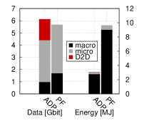
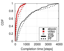
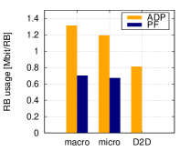
Figure 3: ADP vs. PF: total amount of transferred data and consumed energy (a); CDF of the completion time (b), failed downloads (c), RB usage (d).

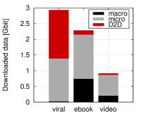
(a) ADP

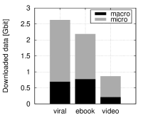
(b) PF

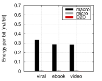
(c) ADP

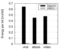
(d) PF

Figure 4: ADP vs. PF: breakdown of the amount of transferred content (a,b), and of the energy consumption per bit of transmitted data (c,d).

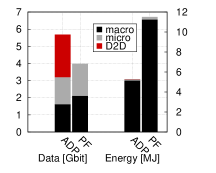
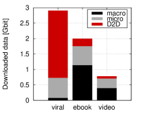
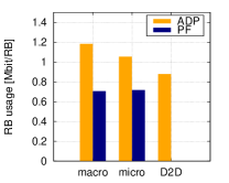
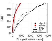
Figure 5: Halving the number of microcells: amount of transferred data and consumed energy (a); amount of transferred data by ADP (b); average RB usage (c); CDF of the completion time (d).

V-C Solution complexity

Recall that our goal is to design a low-complexity solution. This requirement is indeed met. With reference to Fig. 2 (right), and assuming that the dominant factor is the number of users, the complexity is as follows. Step (2), $O(2^{|\mathcal{U}|})$ with plain dynamic programming, which reduces to $O(|\mathcal{U}|)$ using Alg. 3. Steps (3) and (4), linear with $O(|\mathcal{U}|)$. Step (5), $O(1)$. Step (6), $O(|\mathbf{A}|^{k})$ with plain dynamic programming, which reduces to $O(|\mathcal{U}|)$ with Alg. 4.

VI Results

We evaluate our solution in the two-tier scenario that is typically used within 3GPP for LTE network evaluation [21]. The scenario comprises a service network area of 12.34 km², covered by 57 macrocells and, unless otherwise specified, 228 microcells. Macrocells are controlled by 19 three-sector BSs; the macroBSs inter-site distance is set to 500 m. MicroBSs are deployed over the network area, so that there are 4 non-overlapping microcells per macrocell. A total of 3420 users are present in the area. In particular, in order to have a higher user density where microcells are deployed, 10 users are uniformly distributed within 50 m from each microBS. The rest of the users are uniformly distributed over the remaining network area. Users move according to the cave-man model [22], with average speed of 1 m/s. According to current specifications [15, 23], we assume the following pairs of values for power and antenna height: (43 dBm, 25 m) for macroBSs, (30 dBm, 10 m) for microBSs, and (23 dBm, 1.5 m) for UEs. All network nodes operate over a 10 MHz band at 2.6 GHz, thus $|\mathcal{R}|=50$ RBs. As already mentioned, the signal propagation for I2D is modelled according to ITU specifications for urban environment [15] and for D2D according to the specifications in [18], while the SINR is mapped onto per-RB throughput values using the experimental measurements in [20]. The energy consumption of the network nodes is instead computed according to [23].

Users may require content from a set of 21 different items, belonging to three categories: ebooks, videos, or viral content; their characteristics and intervals between user requests are summarized in Table III. We highlight that video and viral items have stricter constraints on delivery time. Additionally, the viral item is modeled as being in high demand to mimic content becoming suddenly popular through social networks (the so-called “flash-crowd” phenomenon).

TABLE III: Content types

Feature	eBook	Video	Viral
No. of items	10	10	1
Size [Mbit]	12	3	3
Deadline [steps]	4000	1000	1000
Request interval [steps]	1–1000	1–1000	41–60

While applying our ADP approach, we consider that the values of the $\alpha_{M},\alpha_{m},\alpha_{u}$ parameters, are discretized as $\{0.1,0.2,\dots,1\}$. Additional experiments with values exhibiting finer granularity have shown negligible improvement. We compare our approach against a system implementing the 3GPP eICIC with a microcell bias of 15 dB and the ABS model where macroBSs are silent in 1 out of every 2 subframes [24]. In the latter, D2D mode is not supported and UEs connect to the BS from which they receive the strongest pilot signal. At the BSs, traffic is scheduled according to the proportional-fairness (PF) algorithm, which is standard in today’s LTE networks [17]. In the following, we will refer to this benchmark scenario as PF.

The first comparison between ADP and PF is presented in Fig. 3. Colors are used to differentiate among the possible endpoints (black for macroBSs, gray for microBSs and red for UEs) and between ADP (orange) and PF (blue). In particular, Fig. 3(a) shows that ADP allows the transfer of more data than the state-of-the-art, while using a much smaller amount of energy. Such a gain is due to the lower usage of macrocells (characterized by very high transmit power), in favour of microcells and D2D. Note that the energy consumption due to D2D mode is negligible and can be barely seen in the plot. Also, under both ADP and PF, transmissions from microBSs are more efficient than those from macroBSs, as the former carry a higher amount of data at a much lower energy cost.

Fig. 3(b) depicts the completion time of successful downloads, for the different content categories (denoted by a different colors). A download is successful if it can be completed by the corresponding deadline. First, note that, since video and viral content have tighter deadlines, they are characterized by better performance than ebooks. Indeed, our cost $\mathbf{C}$ in (V-A) accounts for content deadlines, giving higher priority to those downloads that are closer to their completion deadline. Comparing ADP (solid lines) to PF (dotted lines), we observe that our approach can better meet the time requirements of content with strict deadlines (video and viral), while guaranteeing similar delays for ebooks.

Results in Fig. 3(c) confirm the above observation: ADP can dramatically reduce the number of failed downloads with respect to PF. The only content type for which ADP is unable to deliver some items is video. This due to the fact that, in the traffic scenario under study, video has a quite strict deadline, and it cannot significantly benefit from the D2D mode as users typically ask for different items.

Finally, Fig. 3(d) highlights the improvement in ADP usage of radio resources compared to PF. Observe that, on average, ADP can transmit a higher amount of data per RB, as our interference-aware scheduling assigns endpoints and radio resources far more efficiently than the PF-based system. In other words, ADP scheduling yields higher values of SINR, hence of data rates per RB. This is also underlined by the average number of times an RB is reused in the whole network, whose value normalized to the network area is about 1.58 under ADP and 2.3 under PF. The higher value recorded under PF may at first be surprising, given that ADP allows D2D communication to reuse RBs too. However, such result further underscores the inefficiency of PF in handling interference: it needs to reuse more RBs in order to keep up with traffic demand. At last, looking at different types of endpoints, we note that RBs assigned to macro- and microBS by PF are characterized by similar data rates, in spite of the lower power irradiated by microBS. Such behavior is due to the use of ABS, which mutes macrocells when microcells serve far-away UEs, and to the short distance between microBSs and the other UEs. Conversely, when ADP assigns RBs to microBSs, the difference in data rates between macrocells and microcells flares up. Indeed, D2D communication causes additional interference to UEs served by the cellular infrastructure, which is more significant for microBSs since they transmit at a lower power level. As for D2D mode, it exhibits slightly worse performance than I2D communication. This was expected, since serving UEs transmit at very low power, hence D2D communication is more prone to interference (hence lower SINR and data rate).

Fig. 4 presents the breakdown of delivered data under ADP and PF, on a per-content type basis. In spite of the lower transmission quality, D2D appears to play a crucial role in the delivery of viral content, as shown by Fig. 4(a). Indeed, in case of a peak of social content demand, it is likely that a downloader finds a serving UE within its radio range. Thus, D2D can be effectively used to offload traffic from the cellular infrastructure. On the contrary, PF has to relay on macro- and microBSs only (see Fig. 4(b)). As a consequence, along with a better exploitation of radio resources, ADP requires a much lower energy per transferred data compared to PF, as evident from Figs. 4(c) and (d). In particular, the ADP plot in Fig. 4(c) underscores that the energy consumption due to D2D communication, normalized to the amount of downloaded data, is negligible, thus confirming that D2D mode is a very convenient way to spread social content.

In the scenario above, we now halve the number of microcells from 228 to 114, i.e., 2 microcells per macrocell. The most noticeable effect is that, with ADP, D2D communication steps up to compensate for the missing microBSs, as shown in Fig. 5(a). Instead, PF falls short of providing the same throughput as before. Indeed, comparing to Fig. 3(a), ADP exhibits a mere 8% drop in transferred data, with respect to 30% for PF. Energy consumption increases for both approaches, though ADP still retains a clear edge. A breakdown of per-content data downloaded by ADP (Fig. 3(b)) shows that D2D is even more dominant (by a 32% increase) in viral transfers. In Fig. 5(c), spectrum usage is less effective with the increase in D2D communication: the surging number of D2D links interferes more with macroBSs and the remaining microBSs. Those D2D links whose coverage overlaps one of the missing microcells instead see their amount of transferred bits per RB increase. In Fig. 5(d), viral content relying more on D2D shows the same completion times as before, while video and ebooks experience higher delays. The latter phenomenon is a consequence of the lower number of microcells. Also, ADP tends to favour content with stricter time constraints (viral and video), at the expense of ebooks. For reasons of space, we omit plots comparing other metrics, which however confirm the above observations.

VII Conclusions

We considered a 2-tier, LTE-based network, supporting D2D communication. We devised a solution to the problem of selecting which endpoint should serve a user, and the radio resources to allocate for such communication. In particular, we presented approximate dynamic programming algorithms to generate and rank possible resource allocation decisions. In this way, we obtained a low-complexity solution that can deal with realistic, large-scale scenarios. Our results show the good performance of our solution, as well as the conditions under which D2D communication is more effective. Furthermore, we highlight that D2D mode can be a valid, low-cost alternative to microcells in supporting traffic with little energy consumption.

References

- [1] J. Andrews, “Seven ways that HetNets are a cellular paradigm shift,” IEEE Comm. Mag., 2013.
- [2] C.-H. Yu, K. Doppler, C. B. Ribeiro, and O. Tirkkonen, “Resource sharing optimization for device-to-device communication underlaying cellular networks,” IEEE Trans. on Wireless Comm., 2011.
- [3] M. Zulhasnine, C. Huang, A. Srinivasan, “Efficient resource allocation for device-to-device communication underlaying LTE network,” IEEE WiMob, 2010.
- [4] 3GPP RP-122009, “Study on LTE device to device proximity services,” in 3GPP TSG RAN Meeting #58, Dec. 2012.
- [5] L. Lei, Z. Zhong, C. Lin, X. Shen, “Operator controlled device-to-device communications in LTE-advanced networks,” IEEE Wireless Comm., 2012.
- [6] Freescale white paper, “Next-generation wireless network bandwidth and capacity enabled by heterogeneous and distributed networks,” July 2013.
- [7] Ericsson white paper, “It all comes back to backhaul,” 2012.
- [8] F. Malandrino, C. Casetti, C.-F. Chiasserini, “A fix-and-relax model for heterogeneous LTE-based networks,” IEEE Mascots, 2013.
- [9] H. Elsawy, E. Hossain, D.I. Kim, “HetNets with cognitive small cells: user offloading and distributed channel access techniques,” IEEE Comm. Mag., 2013.
- [10] G. Boudreau et al., “Interference coordination and cancellation for 4G networks,” IEEE Commun. Mag., vol. 47, no. 4, 2009.
- [11] 3GPP Std. Rel. 10, “Enhanced Inter-Cell Interference Control (ICIC) for non-Carrier Aggregation (CA) based deployments of heterogeneous networks for LTE,” RP-100383, June 2013.
- [12] S. Deb, P. Monogioudis, J. Miernik, J.P. Seymour, “Algorithms for enhanced inter-cell interference coordination (eICIC) in LTE HetNets,” IEEE/ACM Trans. on Networking, in press.
- [13] G. Fodor, E. Dahlman, G. Mildh, “Design aspects of network assisted device-to-device communications,” IEEE Comm. Mag., 2012.
- [14] X. Lin, J. G. Andrews, A. Ghosh, “A comprehensive framework for device-to-device communications in cellular networks,” http://arxiv.org/abs/1305.4219.
- [15] ITU-R, “Guidelines for evaluation of radio interface technologies for IMT-Advanced”, Report ITU-R M.2135-1, Dec. 2009.
- [16] B.S. Arnaud, “iPhone slowing down the Internet – Desperate need for 5G R&E networks,” May 2012.
- [17] S. Sesia, I. Toufik, M. Baker (Eds.), LTE – The UMTS long term evolution: From theory to practice, Wiley, 2009.
- [18] J. Meinilä et al., “D5.3: WINNER+ final channel models,” Wireless World Initiative New Radio ‚ WINNER+, 2010.
- [19] W. B. Powell, Approximate dynamic programming, Wiley, 2011.
- [20] D. Martín-Sacristán et al., “3GPP long term evolution: Paving the way towards next 4G,” Waves, 2009.
- [21] 3GPP Technical Report 36.814, “Further advancements for E-UTRA physical layer aspects,” 2010.
- [22] D.J. Watts, Small worlds: The dynamics of networks between order and randomness, Princeton University Press, 1999.
- [23] FP7 IP EARTH project, “Deliverable D2.3: Energy efficiency analysis of the reference systems, areas of improvements and target breakdown,” https://www.ict-earth.eu/.
- [24] A. Ghosh et al., “Heterogeneous cellular networks: From theory to practice,” IEEE Comm. Mag., 2012.