Observables in Loop Quantum Gravity with a cosmological constant

Abstract

An open issue in loop quantum gravity (LQG) is the introduction of a non-vanishing cosmological constant $\Lambda$. In 3d, Chern-Simons theory provides some guiding lines: $\Lambda$ appears in the quantum deformation of the gauge group. The Turaev-Viro model, which is an example of spin foam model is also defined in terms of a quantum group. By extension, it is believed that in 4d, a quantum group structure could encode the presence of $\Lambda\neq 0$.
In this article, we introduce by hand the quantum group ${{\mathcal{U}}_{q}({\mathfrak{s}u}(2))}$ into the LQG framework, that is we deal with ${{\mathcal{U}}_{q}({\mathfrak{s}u}(2))}$-spin networks. We explore some of the consequences, focusing in particular on the structure of the observables. Our fundamental tools are tensor operators for ${{\mathcal{U}}_{q}({\mathfrak{s}u}(2))}$. We review their properties and give an explicit realization of the spinorial and vectorial ones. We construct the generalization of the $\mathrm{U}(N)$ formalism in this deformed case, which is given by the quantum group ${{\mathcal{U}}_{q}({\mathfrak{u}}(n))}$. We are then able to build geometrical observables, such as the length, area or angle operators … We show that these operators characterize a quantum discrete hyperbolic geometry in the 3d LQG case. Our results confirm that the use of quantum group in LQG can be a tool to introduce a non-zero cosmological constant into the theory.

Introduction

Background:

There are different proposals to understand the nature of the cosmological constant $\Lambda$. It can be interpreted as encoding some type of vacuum energy (see stefano1 ; stefano2 ; sola and references therein) or as a coupling constant just like the Newton’s constant $G$. The loop quantum gravity and spinfoam frameworks use the latter interpretation which is motivated by the seminal works of Witten witten-3d , and later of Fock and Rosly fock , and Alekseev, Grosse, Schomerus Alek1 ; Alek2 . Indeed, in a 3d space-time, one can rewrite General Relativity with a (possibly zero) cosmological constant as a Chern-Simons gauge theory. The general phase space structure of the theory for any metric signature and sign of $\Lambda$ can be treated in a nice unified way catherine , using Poisson-Lie groups chari , the classical counterparts of quantum groups. The quantization procedure leads explicitly to a quantum group structure. The full construction, from phase space to quantum group is usually called combinatorial quantization fock ; Alek1 ; Alek2 .
We can also quantize 3d gravity using the spinfoam approach. In this approach, 3d gravity is formulated as a BF theory. When $\Lambda=0$, this is the well-known Ponzano-Regge model (both Euclidian or Lorentzian), based on the irreducible unitary representations of the relevant gauge group. When $\Lambda\neq 0$, the quantum group structure is introduced by hand. The Ponzano-Regge model is deformed, using irreducible unitary representations of the relevant quantum deformation of the gauge group. This is then called the Turaev-Viro model viro . The argument consolidating the incorporation of the cosmological constant into a spinfoam model through a quantum group comes from the semi-classical limit. Indeed, the asymptotics of the deformed $\{6j\}_{q}$ symbol, entering into the definition of the Turaev-Viro model, goes to the Regge action with a cosmological constant in the regime $\ell_{p}\ll\ell\ll R$.
The third approach to quantize gravity is the canonical approach, i.e.  the loop quantum gravity approach (LQG). In this case, performing the classical hamiltonian analysis to General Relativity, the cosmological constant only appears in the Hamiltonian constraint. This means that the kinematical space is the same whether $\Lambda=0$ or not. In particular this kinematical space (where the Gauss constraint has been solved) is based on the classical relevant gauge group.

Therefore at this stage, quantum groups naturally appear only in the combinatorial quantization of Chern-Simons. Different quantum groups are revealed according to the metric signature and the sign of the cosmological constant. When $\Lambda\neq 0$, we obtain $q$-deformed version of the gauge group ${\mathcal{U}}_{q}(\mathfrak{g})$, where $\mathfrak{g}$ is the Lie algebra of the gauge group $G=\mathrm{SL}(2,{\mathbb{R}})$ in the Lorentzian case, $\mathrm{SU}(2)$ in the Euclidean case, with $q$ function of the Planck scale and the cosmological radius $R=\sqrt{|\Lambda|}$. The deformation parameter $q$ can be real or complex. A nice way to recall what is $q$ according to the sign of $\Lambda$ and the signature is to consider $q=exp\left({-\frac{\hbar G\sqrt{\Lambda}}{\sqrt{c^{2}}}}\right)$ and posing $c^{2}>0$ in the Lorentzian case and $c^{2}<0$ in the Euclidian case bernd . Note that this trick gives $q$ or $q^{-1}$. The full relevant quantum group arising from the combinatorial quantization is ${\mathcal{D}}({\mathcal{U}}_{q}(\mathfrak{g}))$, the Drinfeld double of ${\mathcal{U}}_{q}(\mathfrak{g})$. When $\Lambda=0$, we get the Drinfeld double ${\mathcal{D}}({\mathcal{U}}(\mathfrak{g}))$ with a non-commutative parameter given by $\kappa=\ell_{p}$ in units $\hbar=1=c$. A list of the different quantum groups relevant for 3d gravity is given in the first table below.

Since classically, the Chern-Simons formulation and the standard formulation of General Relativity are equivalent (modulo the degenerated metrics), we can wonder whether the Chern-Simons combinatorial quantization formalism, LQG and the spinfoam framework are related in some ways. It can be shown explicitly in the Euclidian case, with $\Lambda>0$, that the Chern-Simons quantum model and the Turaev-Viro model are related, more precisely, the Turaev Viro amplitude is the square of the Chern-Simons amplitude CS-TV . On the other hand, it seems difficult to relate the LQG formalism, when $\Lambda\neq 0$, to a spin foam model based on a quantum group if we assume that the LQG kinematical space is based on a classical group such as $\mathrm{SU}(2)$.

When $\Lambda=0$, it is also possible to relate the Chern-Simons amplitude and the Ponzano Regge amplitude louapre , which allows to identify a hidden symmetry given by the Drinfeld double ${\mathcal{D}}({\mathcal{U}}(\mathfrak{g}))$ in the Ponzano-Regge model. Still when $\Lambda=0$, explicit links between LQG and the spinfoam framework ale-karim or between the Chern Simons combinatorial quantization and LQG karim-cat have been identified. Note also that we can identify a hidden quantum group structure (the Drinfeld double) in LQG when $\Lambda=0$ louapre ; karim ; karim-cat , which is consistent with the other approaches. The different cases for 3d gravity are summarized in the first table. For more details, we refer to the excellent review bernd .

Signature	$\Lambda$	Quantum group	QG models
Euclidian Lorentzian	$\Lambda>0$ $\Lambda=0$ $\Lambda<0$ $\Lambda>0$ $\Lambda=0$ $\Lambda<0$	${\mathcal{D}}({{\mathcal{U}}_{q}({\mathfrak{s}u}(2))})$, $q=e^{i\frac{\ell_{p}}{R}}$ ${\mathcal{D}}({\mathcal{U}}({\mathfrak{s}u}(2)))$, $\kappa=\ell_{p}$ ${\mathcal{D}}({{\mathcal{U}}_{q}({\mathfrak{s}u}(2))})$, $q=e^{\frac{\ell_{p}}{R}}$ ${\mathcal{D}}({\mathcal{U}}_{q}({\mathfrak{s}l}(2,{\mathbb{R}})))$, $q=e^{-\frac{\ell_{p}}{R}}$ ${\mathcal{D}}({\mathcal{U}}({\mathfrak{s}l}(2,{\mathbb{R}})))$, $\kappa=\ell_{p}$ ${\mathcal{D}}({\mathcal{U}}_{q}({\mathfrak{s}l}(2,{\mathbb{R}})))$, $q=e^{-i\frac{\ell_{p}}{R}}$	Chern-Simons $\stackrel{{\scriptstyle\text{\cite[cite]{\@@bibref{Authors Phrase1YearPhrase2}{CS-TV}{\@@citephrase{(}}{\@@citephrase{)}}}}}}{{{\leftrightarrow}}}$ Turaev-Viro $\stackrel{{\scriptstyle?}}{{\leftrightarrow}}$ LQG Chern-Simons $\stackrel{{\scriptstyle\text{\cite[cite]{\@@bibref{Authors Phrase1YearPhrase2}{louapre}{\@@citephrase{(}}{\@@citephrase{)}}}}}}{{\leftrightarrow}}$ Ponzano-Regge$\stackrel{{\scriptstyle\text{\cite[cite]{\@@bibref{Authors Phrase1YearPhrase2}{ale-karim}{\@@citephrase{(}}{\@@citephrase{)}}}}}}{{\leftrightarrow}}$ LQG $\stackrel{{\scriptstyle\text{\cite[cite]{\@@bibref{Authors Phrase1YearPhrase2}{karim-cat}{\@@citephrase{(}}{\@@citephrase{)}}}}}}{{\leftrightarrow}}$ Chern-Simons Chern-Simons $\stackrel{{\scriptstyle?}}{{\leftrightarrow}}$ Turaev-Viro $\stackrel{{\scriptstyle?}}{{\leftrightarrow}}$ LQG Chern-Simons $\stackrel{{\scriptstyle?}}{{\leftrightarrow}}$ Turaev-Viro $\stackrel{{\scriptstyle?}}{{\leftrightarrow}}$ LQG Chern-Simons $\stackrel{{\scriptstyle\text{\cite[cite]{\@@bibref{Authors Phrase1YearPhrase2}{louapre}{\@@citephrase{(}}{\@@citephrase{)}}}}}}{{\leftrightarrow}}$ Ponzano-Regge$\stackrel{{\scriptstyle\text{\cite[cite]{\@@bibref{Authors Phrase1YearPhrase2}{ale-karim}{\@@citephrase{(}}{\@@citephrase{)}}}}}}{{\leftrightarrow}}$ LQG $\stackrel{{\scriptstyle\text{\cite[cite]{\@@bibref{Authors Phrase1YearPhrase2}{karim-cat}{\@@citephrase{(}}{\@@citephrase{)}}}}}}{{\leftrightarrow}}$ Chern-Simons Chern-Simons $\stackrel{{\scriptstyle?}}{{\leftrightarrow}}$ Turaev-Viro $\stackrel{{\scriptstyle?}}{{\leftrightarrow}}$ LQG

When dealing with 4d space-time, there is no Chern-Simons theory to guide us. Hence, it is postulated that the cosmological constant should also be introduced through a quantum group structure. From the spinfoam approach, one then considers the model one prefers (Barrett-Crane (BC) or EPRL-FK) when $\Lambda=0$, based on the irreducible unitary representations of the gauge group and one deforms it yetter ; roche ; winston ; muxin0 . To argue a posteriori, that this is the right thing to do, we can look at the asymptotic of the spinfoam amplitude and check we recover the Regge action with a cosmological constant limits . It is quite interesting that the current ”physical” EPRL spinfoam model defined in the Lorentzian case, with $\Lambda>0$ leads to a finite amplitude winston ; muxin0 .

In 4d, we are not able to connect the Hamiltonian constraint arising in LQG to a spinfoam model, even when $\Lambda=0$. Just as in 3d, it is not clear at all why a quantum group structure should appear in the LQG framework. There exist few arguments to justify this postulate pranzetti . We include now a table summarizing the different quantum group models appearing in 4d quantum gravity.

Signature	$\Lambda$	Quantum group	QG models
Euclidian Lorentzian	$\Lambda>0$ $\Lambda=0$ $\Lambda<0$ $\Lambda>0$ $\Lambda=0$ $\Lambda<0$	${\mathcal{U}}_{q}({\mathfrak{s}o}(4))$, $q=e^{i2\pi{\ell^{2}_{p}}{\Lambda}}$ ? ${\mathcal{U}}_{q}({\mathfrak{s}o}(4))$, $q=e^{i2\pi\frac{\ell^{2}_{p}}{\Lambda}}$ ${\mathcal{U}}_{q}({\mathfrak{s}o}(3,1))$, $q=e^{{\ell^{2}_{p}}{\Lambda}}$ ? ${\mathcal{U}}_{q}({\mathfrak{s}o}(3,1))$, $q=e^{\frac{\ell^{2}_{p}}{\Lambda}}$	BC or EPRL-FK $\stackrel{{\scriptstyle?}}{{\Leftrightarrow}}$ LQG BC or EPRL-FK $\stackrel{{\scriptstyle?}}{{\Leftrightarrow}}$ LQG BC or EPRL-FK $\stackrel{{\scriptstyle?}}{{\Leftrightarrow}}$ LQG BC or EPRL-FK $\stackrel{{\scriptstyle?}}{{\Leftrightarrow}}$ LQG BC or EPRL-FK $\stackrel{{\scriptstyle?}}{{\Leftrightarrow}}$ LQG BC or EPRL-FK $\stackrel{{\scriptstyle?}}{{\Leftrightarrow}}$ LQG

Several remarks can be made at this stage. The partition function of the Plebanski action is invariant under the transformation $\Lambda\rightarrow-\Lambda$ de pietri freidel , which explains why we have the same quantum group for the different signs of the cosmological constant. This change of sign for $\Lambda$ is equivalent to $q\rightarrow q^{{-1}}$.

In the ”physical” case (Lorentzian, $\Lambda>0$) in the EPRL-FK model, spin networks encoding the quantum state of space are defined in terms of ${{\mathcal{U}}_{q}({\mathfrak{s}u}(2))}$, with $q$ real winston ; muxin0 .

We also emphasize en passant, that the quantum deformation of the Lorentz group (in 3d or 4d) for $q$ complex are not understood.

Motivations:

A common feature of the 3d and 4d quantum gravity is that it is hard to understand why a $q$-deformation of the gauge group would appear from the LQG perspective. Since we do not know how to solve the Hamiltonian constraint (for $\Lambda\neq 0$) and since we would like to compare the LQG approach with the well-known models coming from combinatorial quantization formalism and spinfoam, we would like to define LQG with a $q$-deformed group and see what the consequences are. We hope then to identify some hints pointing to the quantum group apparition in this context. In particular, if LQG defined in terms of a quantum group describes well quantum curved geometries, then this is a good sign that this could be a useful theory to consider.

To this aim, we need to understand the structure of the observables associated to spin networks defined using the representations of a quantum group. Not much work has been done in this context: LQG with a quantum group has only been explored using the loop variables by Major and Smolin major1 ; major2 ; major3 .

When $\Lambda=0$, the structure of the observables for a spin network (or an intertwinner) is well understood, thanks to the spinor approach to LQG un0 ; un1 ; un2 . In particular it is possible to construct a closed algebra (a ${\mathfrak{u}}(n)$ Lie algebra, where $n$ is the number of intertwinner legs) that generates all the observables acting on an intertwinner. This approach not only gives some information about the observable structure but it has been applied to different contexts, with many interesting results un0 ; un1 ; un2 . This formalism has helped to understand that spin networks can be seen as the quantization of classical discrete geometries, the so called twisted geometries twisted1 ; twisted2 . It allowed the construction of a new Hamiltonian constraint in 3d Euclidian gravity valentin-etera , such that the kernel of this constraint is given by the $6j$ symbol, i.e.  the Ponzano-Regge amplitude. It has provided the tools to implemented in a rigorous way the simplicity constraints, using the Gupta-Bleuler method, to build a spinfoam model for Euclidian gravity ($\Lambda=0$) maite1 .

Generalizing the spinor formalism to the quantum group case will help to better understand the quantum gravity regime with a nonzero cosmological constant. Indeed, within this formalism, we should be able to construct an Hamiltonian constraint relating Turaev-Viro and LQG hamiltonian , and we should be able to understand what is the relevant phase space for LQG, the space of curved twisted geometries phase space .

Main results:

This generalization of the spinor formalism to the quantum group case is the main result of this paper. We have focused on the quantum group ${{\mathcal{U}}_{q}({\mathfrak{s}u}(2))}$ with $q$ real, which is therefore relevant for 3d Euclidian gravity with $\Lambda<0$ and the physical case, i.e.  4d Lorentzian gravity with $\Lambda>0$.

The key idea for this generalization is the use of tensor operators. These are well-known in the quantum mechanical case for $\mathrm{SU}(2)$ sakurai . Essentially, they are sets of operators that transform well under $\mathrm{SU}(2)$, i.e.  as a representation. They are known in LQG under the name of grasping operators. However they have not been studied intensively in this context. We show that considering these operators seriously naturally leads to the spinor approach to LQG. These tensor operators can be generalized to the quantum group case (more exactly they are defined for any quasi-triangular Hopf algebra) rittenberg .

Given an ${{\mathcal{U}}_{q}({\mathfrak{s}u}(2))}$ intertwinner with $n$ legs, we have identified some sets of operators that transform well under ${{\mathcal{U}}_{q}({\mathfrak{s}u}(2))}$. Due to the quantum group structure, they are much more complicated than their classical counterparts. In particular their commutation relations are pretty complicated. We have clarified the construction of ${{\mathcal{U}}_{q}({\mathfrak{s}u}(2))}$ intertwinner observables. We show how there exists a fundamental algebra generating all observables, which is a deformation of the ${\mathfrak{u}}(n)$ algebra. We also discuss the geometric interpretation of some observables for 3d Euclidian LQG with $\Lambda<0$, pinpointing the fact that the quantum group structure encodes as expected the notion of curved discrete geometry. Some of these results were already announced in ours .

Outline of the paper:

The paper is organized as follow. In section I, we recall the main features of ${{\mathcal{U}}_{q}({\mathfrak{s}u}(2))}$, the $q$-deformed universal enveloping algebra of $\mathrm{SU}(2)$, with $q$ real. We recall as well the notion of $q$-harmonic oscillators which are used to build some tensor operators explicit realizations.

Section II is a review about tensor operators for ${{\mathcal{U}}_{q}({\mathfrak{s}u}(2))}$, the essential tools of our construction. Due to the nonlinearity of the quantum group structure, ${{\mathcal{U}}_{q}({\mathfrak{s}u}(2))}$ tensor operators are more complicated than the standard $\mathrm{SU}(2)$ case. In particular, due to the nontrivial nature of the quantum group action, the tensor product of tensor operators is highly nontrivial, which will make the construction of tensor operators acting on different legs of an intertwiner quite cumbersome, but necessary.

Different explicit realizations of tensor operators for ${{\mathcal{U}}_{q}({\mathfrak{s}u}(2))}$ are given in section III. We recalled the results of Quesnes quesne regarding spinor operators: their definition in terms of $q$-harmonic oscillators and their commutation relations for spinor operators acting on different legs. We have extended this analysis to vector operators, which will be relevant for the construction of the standard geometric operators.

The main results of this paper are presented in section IV and V. We discuss the general construction of observables for a ${{\mathcal{U}}_{q}({\mathfrak{s}u}(2))}$ intertwiner. We construct a new realization of ${{\mathcal{U}}_{q}({\mathfrak{u}}(n))}$ in terms of tensor operators, which is also invariant under the action of ${{\mathcal{U}}_{q}({\mathfrak{s}u}(2))}$. We have identified the non-linear map relating our invariant operators to the standard ${{\mathcal{U}}_{q}({\mathfrak{u}}(n))}$ Weyl-Cartan generators. We construct different geometric operators which we interpret in the context of 3d Euclidian LQG with $\Lambda<0$. We show how we get a quantization of the hyperbolic cosine law, a quantization of the length and of the area of a triangle. We pinpoint also how the presence of the cosmological constant allows for a notion of minimum angle.

In the concluding section, we discuss the possible follow-ups of this tensor operator approach to LQG.

We have also included some appendices to recall the definition of the hyperbolic cosine law as well as some relevant formulae regarding the ${{\mathcal{U}}_{q}({\mathfrak{s}u}(2))}$ recoupling coefficients.

I ${{\mathcal{U}}_{q}({\mathfrak{s}u}(2))}$ in a nutshell

I.1 Definition of ${{\mathcal{U}}_{q}({\mathfrak{s}u}(2))}$

In this section, we review the salient features of ${{\mathcal{U}}_{q}({\mathfrak{s}u}(2))}$, which we shall extensively use, to fix the notations. We consider ${{\mathcal{U}}_{q}({\mathfrak{s}u}(2))}$, the $q$-deformation of the universal algebra of $\mathrm{SU}(2)$, with $q$ real, generated by $J_{z},\;J_{+},\;J_{-}$. We have the commutation relations

$$[J_{z},J_{\pm}]=\pm J_{\pm},\quad[J_{+},J_{-}]=[2J_{z}],\textrm{ with }[J_{z}]=\frac{q^{J_{z}/2}-q^{-J_{z}/2}}{q^{1/2}-q^{-1/2}}.$$ (1)

For $q\rightarrow 1$ the right-hand side of the second equation of (1) approaches $2J_{z}$ and we thus recover the usual Lie algebra ${\mathfrak{s}u}(2)$. ${{\mathcal{U}}_{q}({\mathfrak{s}u}(2))}$ is equipped with a structure of quasitriangular Hopf algebra $(\Delta,\epsilon,S,\mathcal{R})$ chari ; majid ; kassel .

• The coproduct $\Delta:{{\mathcal{U}}_{q}({\mathfrak{s}u}(2))}\rightarrow{{\mathcal{U}}_{q}({\mathfrak{s}u}(2))}\otimes{{\mathcal{U}}_{q}({\mathfrak{s}u}(2))}$ encodes physically the total angular momentum of a 2-particle system.

  $$\Delta J_{z}=J_{z}\otimes{\bf 1}+{\bf 1}\otimes J_{z},\quad\Delta J_{\pm}=J_{\pm}\otimes q^{J_{z}/2}+q^{-J_{z}/2}\otimes J_{\pm}.$$ (2)

  Considering the un-deformed case, we have

  $$(\Delta J_{\sigma})\,|j_{1}m_{1},j_{2}m_{2}\rangle=(J_{\sigma}\otimes{\bf 1}+{\bf 1}\otimes J_{\sigma})|j_{1}m_{1}j_{2}m_{2}\rangle=(J_{\sigma}^{(1)}+J_{\sigma}^{(2)})|j_{1}m_{1}j_{2}m_{2}\rangle,\;\textrm{ where }\sigma=+,\,-,\,z.$$ (3)

  In the deformed case, the addition of angular momenta (2) is non-commutative, hence the addition of $q$-angular momenta depends on the order we set our particles. As we shall see, the braiding constructed using the $\mathcal{R}$-matrix will allow to relate different orderings.

• The counit $\epsilon:{{\mathcal{U}}_{q}({\mathfrak{s}u}(2))}\rightarrow{{\mathcal{U}}_{q}({\mathfrak{s}u}(2))}$ is defined such that $\epsilon(\mathbb{I})=1,\,\epsilon(J_{\sigma})=0$ for $\sigma=+,\,-,\,z$.

• The antipode $S:{{\mathcal{U}}_{q}({\mathfrak{s}u}(2))}\rightarrow{{\mathcal{U}}_{q}({\mathfrak{s}u}(2))}$ encodes in some sense the notion of inverse angular momentum.

  $$SJ_{z}=-J_{z},\quad SJ_{\pm}=-q^{\pm 1/2}J_{\pm}.$$ (4)

• The $\mathcal{R}$-matrix encodes the ”amount” of non-commutativity of the coproduct, i.e.   of the addition of angular momenta. Indeed, if we note $\psi:{{\mathcal{U}}_{q}({\mathfrak{s}u}(2))}\otimes{{\mathcal{U}}_{q}({\mathfrak{s}u}(2))}\rightarrow{{\mathcal{U}}_{q}({\mathfrak{s}u}(2))}\otimes{{\mathcal{U}}_{q}({\mathfrak{s}u}(2))}$, the permutation, then we have that

  $$(\psi\circ\Delta)X={\mathcal{R}}(\Delta X){\mathcal{R}}^{{-1}}.$$ (5)

  In terms of the ${{\mathcal{U}}_{q}({\mathfrak{s}u}(2))}$-generators, the $\mathcal{R}$-matrix can be written as

  $$\mathcal{R}=\sum{\mathcal{R}}_{1}\otimes{\mathcal{R}}_{2}=q^{J_{z}\otimes J_{z}}\sum_{n=0}^{\infty}\frac{(1-q^{-1})^{n}}{[n]!}q^{n(n-1)/4}(q^{J_{z}/2}J_{+})^{n}\otimes(q^{-J_{z}/2}J_{-})^{n},$$ (6)

  where $[n]$ denotes the $q$-number $[n]\equiv\frac{q^{\frac{n}{2}}-q^{-\frac{n}{2}}}{q^{\frac{1}{2}}-q^{-\frac{1}{2}}}$. A co-commutative product would simply mean that ${\mathcal{R}}={\bf 1}\otimes{\bf 1}$, which is obtained when $q\rightarrow 1$ in (6). Further properties of the ${\mathcal{R}}$-matrix are given in the Appendix B, in particular its expression in terms of Clebsch-Gordan coefficients.

  The non-co-commutativity of the coproduct implies that we have a ”non-commutative” tensor product. Essentially, we would get a symmetric 2-particle system if the permutation of the particles states does not affect the total observable, that is the permutation leaves invariant the coproduct, $\psi\circ\Delta=\Delta$.

  If it is non-co-commutative, as in the ${{\mathcal{U}}_{q}({\mathfrak{s}u}(2))}$ case, we can still define a deformed permutation $\psi_{{\mathcal{R}}}$ – thanks to the existence of the ${\mathcal{R}}$-matrix rittenberg ; kassel .

  $$\psi_{{\mathcal{R}}}:V\otimes W \rightarrow W\otimes V$$

  $$v\otimes w \rightarrow \psi_{{\mathcal{R}}}(|v,w\rangle)\equiv\psi({\mathcal{R}}|v,w\rangle)=\sum\psi(|{\mathcal{R}}_{1}v,{\mathcal{R}}_{2}w\rangle)=\sum|{\mathcal{R}}_{2}w,{\mathcal{R}}_{1}v\rangle.$$ (7)

  Using the key property $(\psi\circ\Delta)X={\mathcal{R}}(\Delta X){\mathcal{R}}^{{-1}}$, we have that

  $$\psi_{{\mathcal{R}}}(X(|v,w\rangle))=\psi({\mathcal{R}}X(|v,w\rangle))=\psi({\mathcal{R}}(\Delta X)|v,w\rangle)=\psi((\psi\circ\Delta X){\mathcal{R}}|v,w\rangle)=(\Delta X)\psi({\mathcal{R}}|v,w\rangle)=X(\psi_{{\mathcal{R}}}(|v,w\rangle)).$$

  Hence, the tensor product is only symmetric under this deformed notion of permutation. From now on, we shall always consider this deformed permutation $\psi_{{\mathcal{R}}}$ which is the natural notion of permutation in this quasi-triangular context.

The representation theory of ${{\mathcal{U}}_{q}({\mathfrak{s}u}(2))}$ with $q$ real is very similar to the one of ${\mathfrak{s}u}(2)$ BiedenharnBook . A representation $V^{j}$ is generated by the vectors $|j,m\rangle$ with $j\in{\mathbb{N}}/2$ and $m\in\left\{-j,..,j\right\}$. The key-difference is that the action of the generators on these vectors generates $q$-numbers.

$$J_{z}\,|jm\rangle=m\;|jm\rangle,$$ (8)

$$J_{\pm}\,|jm\rangle=\sqrt{[j\mp m][j\pm m+1]}\;|{j}{m\pm 1}\rangle.$$ (9)

A Casimir operator can be defined as

$$C=J_{+}J_{-}+[J_{z}][J_{z}-1]=J_{-}J_{+}+[J_{z}][J_{z}+1].$$ (10)

The tensor product of vectors $|j_{1}m_{1},j_{2}m_{2}\rangle$ can be decomposed into a linear combination of vectors using the $q$-Clebsh-Gordon (CG) coefficients $\,{}_{q}\textbf{C}\begin{array}[]{c@{}c@{}c}j_{1}&j_{2}&j\\ m_{1}&m_{2}&m\end{array}$.

$$|j_{1}m_{1},j_{2}m_{2}\rangle={\sum_{j,m}}\,\,_{q}\textbf{C}\begin{array}[]{c@{}c@{}c}j_{1}&j_{2}&j\\ m_{1}&m_{2}&m\end{array}|jm\rangle,\quad j=|j_{1}-j_{2}|,..,j_{1}+j_{2}.$$ (13)

Conversely, given a representation $V^{j}$ of ${{\mathcal{U}}_{q}({\mathfrak{s}u}(2))}$ we can decompose it along two representations $V^{j_{1}}$ and $V^{j_{2}}$ of ${{\mathcal{U}}_{q}({\mathfrak{s}u}(2))}$ (with $|j_{1}-j_{2}|\leq j\leq j_{1}+j_{2}$ )

$$|jm\rangle=\sum_{m_{1},m_{2}}\,\,{}_{q}\textbf{C}\begin{array}[]{c@{}c@{}c}j_{1}&j_{2}&j\\ m_{1}&m_{2}&m\end{array}|j_{1}m_{1},j_{2}m_{2}\rangle.$$ (14)

Acting with a generator $J_{\sigma}\,(\sigma=+,-,z)$ on the righthand side of (13) and with its coproduct on the lefthand side of (13) we obtain a recursion relation for the CG coefficients BiedenharnBook . Such recursion relations can be taken as defining the CG coefficients.

$$J_{z}\,\triangleright|j_{1}m_{1},j_{2}m_{2}\rangle={\sum_{j,m}}\,\,_{q}\textbf{C}\begin{array}[]{c@{}c@{}c}j_{1}&j_{2}&j\\ m_{1}&m_{2}&m\end{array}J_{z}\,\triangleright|jm\rangle\Leftrightarrow\Delta J_{z}\,|j_{1}m_{1},j_{2}m_{2}\rangle={\sum_{j,m}}\,\,_{q}\textbf{C}\begin{array}[]{c@{}c@{}c}j_{1}&j_{2}&j\\ m_{1}&m_{2}&m\end{array}J_{z}\,|jm\rangle$$ (19)

$$\qquad\qquad\qquad\qquad\Rightarrow\;m_{1}+m_{2}=m$$

$$J_{\pm}\,\triangleright|j_{1}m_{1},j_{2}m_{2}\rangle={\sum_{j,m}}\,\,_{q}\textbf{C}\begin{array}[]{c@{}c@{}c}j_{1}&j_{2}&j\\ m_{1}&m_{2}&m\end{array}J_{\pm}\,\triangleright|jm\rangle\Leftrightarrow\Delta J_{\pm}\,|j_{1}m_{1},j_{2}m_{2}\rangle={\sum_{j,m}}\,\,_{q}\textbf{C}\begin{array}[]{c@{}c@{}c}j_{1}&j_{2}&j\\ m_{1}&m_{2}&m\end{array}J_{\pm}\,|jm\rangle$$ (24)

$$\quad\Rightarrow\;q^{-\frac{m_{1}}{2}}\left([j_{2}\pm m_{2}][j_{2}\mp m_{2}+1]\right)^{\frac{1}{2}}\,_{q}\textbf{C}\begin{array}[]{c@{}c@{}c}j_{1}&j_{2}&j\\ m_{1}&m_{2}\mp 1&m\end{array}+q^{\frac{m_{2}}{2}}\left([j_{1}\pm m_{1}][j_{1}\mp m_{1}+1]\right)^{\frac{1}{2}}\,_{q}\textbf{C}\begin{array}[]{c@{}c@{}c}j_{1}&j_{2}&j\\ m_{1}\mp 1&m_{2}&m\end{array}$$ (29)

$$\qquad\qquad\qquad\qquad\qquad=\left([j\mp m][j\pm m+1]\right)^{\frac{1}{2}}\,_{q}\textbf{C}\begin{array}[]{c@{}c@{}c}j_{1}&j_{2}&j\\ m_{1}&m_{2}&m\pm 1\end{array}.$$ (32)

We refer to the Appendix B for further CG coefficients relevant properties.

Let us now introduce the notion of intertwiner for ${{\mathcal{U}}_{q}({\mathfrak{s}u}(2))}$ which is a fundamental object in LQG. An intertwinner is a vector $|\iota_{j_{1}..j_{N}}\rangle=\sum_{m_{i}}c_{m_{1}..m_{N}}|j_{1}m_{1},..,j_{N}m_{N}\rangle\in V^{j_{1}}\otimes..\otimes V^{j_{N}}$ which is invariant under the action of ${{\mathcal{U}}_{q}({\mathfrak{s}u}(2))}$.

$$J_{\alpha}\triangleright|\iota_{j_{1}..j_{N}}\rangle=\left[({\bf 1}\otimes..{\bf 1}\otimes\Delta)\circ..\circ({\bf 1}\otimes\Delta)\circ\Delta\right](J_{\alpha})|\iota_{j_{1}..j_{N}}\rangle=0,\;\alpha=\pm,z.$$ (33)

Note that since the coproduct is co-associative, we have no issue on how to compose the coproducts. In the case of $N=3$, (33) is equivalent to the recursion relations which define the CG coefficients. A normalized 3-valent intertwiner is then uniquely defined by

$$|\iota_{j_{1}j_{2}j_{3}}\rangle=\sum_{m_{i}}\frac{(-1)^{j_{3}-m_{3}}q^{-\frac{m_{3}}{2}}}{[2j_{3}+1]^{\frac{1}{2}}}\,_{q}\textbf{C}\begin{array}[]{c@{}c@{}c}j_{1}&j_{2}&j_{3}\\ m_{1}&m_{2}&-m_{3}\end{array}|j_{1}m_{1},j_{2}m_{2},j_{3}m_{3}\rangle.$$ (36)

Another ingredient which we shall use extensively in the following sections, is the adjoint action of ${{\mathcal{U}}_{q}({\mathfrak{s}u}(2))}$ on an operator ${\mathcal{O}}$. It differs from the usual adjoint action of ${\mathfrak{s}u}(2)$ given by a commutator. The ${{\mathcal{U}}_{q}({\mathfrak{s}u}(2))}$ adjoint action of the generators $J_{\sigma}$ is explicitly given by

$$J_{z}\triangleright{\mathcal{O}}=[J_{z},{\mathcal{O}}],\quad J_{\pm}\triangleright{\mathcal{O}}=J_{\pm}{\mathcal{O}}q^{-J_{z}/2}-q^{\pm\frac{1}{2}}q^{-J_{z}/2}{\mathcal{O}}J_{\pm}.$$ (37)

The following lemma is useful to relate quantities which are invariant under the adjoint action and the different Casimir one can construct. This is especially relevant in our case since the commutator and the adjoint action are not coinciding.

Lemma I.1.

Let ${\mathcal{C}}\in{{\mathcal{U}}_{q}({\mathfrak{s}u}(2))}$ invariant under the adjoint action, then ${\mathcal{C}}$ commutes with the generators $J_{\sigma}$, $\sigma=+,-,z$. Conversely, if ${\mathcal{C}}\in{{\mathcal{U}}_{q}({\mathfrak{s}u}(2))}$ commutes with $J_{\sigma}$, then it is invariant under the adjoint action.

I.2 $q$-harmonic oscillators and the Schwinger-Jordan trick

To account for the deformation, we consider a pair of $q$-harmonic oscillators, comprising annihilation operators $\alpha_{i}=a,b$, creation operators $\alpha^{\dagger}_{i}=a^{\dagger},b^{\dagger}$ and number operators $N_{\alpha_{i}}=N_{a},N_{b}$, to construct representations of ${{\mathcal{U}}_{q}({\mathfrak{s}u}(2))}$. There are defined as follows,

$$[\alpha_{i},\alpha_{j}]=[\alpha_{i},\alpha_{j}^{\dagger}]=0,\textrm{ with }i\neq j,\quad[\alpha_{i},\alpha_{i}^{\dagger}]_{q^{\pm\frac{1}{2}}}=q^{\frac{\mp N_{\alpha_{i}}}{2}},\quad[N_{\alpha_{i}},\alpha_{j}^{\dagger}]=\delta_{{ij}}\alpha_{i}^{\dagger},\quad[N_{\alpha_{i}},\alpha_{j}]=-\delta_{{ij}}\alpha_{i},$$ (38)

where $[A,B]_{q^{n}}\equiv AB-q^{n}BA$. Let us point out that the operator $\alpha_{i}^{\dagger}\alpha_{i}$ is not the number operator $N_{\alpha_{i}}$ but rather is equal to $[N_{\alpha_{i}}]$. From (38), we have also that

$$q^{N_{\alpha_{i}}/2}\alpha_{i}^{\dagger}=q^{1/2}\alpha_{i}^{\dagger}q^{N_{\alpha_{i}}/2},\quad q^{N_{\alpha_{i}}/2}\alpha_{i}=q^{-1/2}\alpha_{i}q^{N_{\alpha_{i}}/2},\quad\alpha_{i}^{\dagger}\alpha_{i}=[N_{\alpha_{i}}],\quad\alpha_{i}\alpha_{i}^{\dagger}=[N_{\alpha_{i}}+1].$$ (39)

The harmonic oscillator $\alpha_{i}$, $\alpha_{i}^{\dagger}$, $N_{\alpha_{i}}$ acts on the Fock space $F_{i}=\{\sum_{n_{i}}c_{n_{i}}|n_{i}\rangle\}$ with vacuum $|0\rangle$.

$$\alpha_{i}|0\rangle=0,\quad\alpha_{i}|n_{i}\rangle=\sqrt{[n_{i}]}|n_{i}-1\rangle,\,\textrm{ with }n_{i}\geq 1,\quad\textrm{ and }\alpha_{i}^{\dagger}|n_{i}\rangle=\sqrt{[n_{i}+1]}|n_{i}+1\rangle.$$ (40)

The generators of ${{\mathcal{U}}_{q}({\mathfrak{s}u}(2))}$ can be realized in terms of the pair of $q$-harmonic oscillators $(a,b)$, their adjoint and their number operator macfarl ; bienden .

$$J_{z}=\frac{1}{2}(N_{a}-N_{b}),\quad J_{+}=a^{\dagger}b,\quad J_{-}=b^{\dagger}a,\quad C=[\frac{1}{2}(N_{a}+N_{b})][\frac{1}{2}(N_{a}+N_{b})+1].$$ (41)

Using this representation together with (38), we can recover the commutation relations (1). We can also use the Fock space $F\sim F_{{a}}\otimes F_{b}=\{\sum c_{n_{a}n_{b}}|n_{a},n_{b}\rangle,\;c_{n_{a}n_{b}}\in{\mathbb{R}}\}$ of this pair of $q$-harmonic oscillators to generate the representations of ${{\mathcal{U}}_{q}({\mathfrak{s}u}(2))}$ by setting

$$j=\frac{1}{2}(n_{a}+n_{b}),\quad m=\frac{1}{2}(n_{a}-n_{b}).$$ (42)

The states $|jm\rangle$ are then homogenous polynomials in the operators $\alpha_{i},\,\alpha_{i}^{\dagger}$.

$$|jm\rangle=\frac{\left(a^{\dagger}\right)^{j+m}\left(b^{\dagger}\right)^{j-m}}{\sqrt{[j+m]![j-m]!}}|0,0\rangle.$$ (43)

II Tensor operators for ${{\mathcal{U}}_{q}({\mathfrak{s}u}(2))}$

We now introduce the concept of tensor operators. The general definition of tensor operators for a general quasitriangular Hopf algebra has been given in rittenberg . We use their formalism in the specific case of ${{\mathcal{U}}_{q}({\mathfrak{s}u}(2))}$. These objects are the building blocks of our construction of observables for LQG defined with ${{\mathcal{U}}_{q}({\mathfrak{s}u}(2))}$ as gauge group. We show in section IV that the use of tensor operators allows us to build any observables associated to an intertwiner (of a quantum or a classical group) in a straightforward manner.

II.1 Definition and Wigner-Eckart theorem

Definition II.1.

Tensor operators rittenberg .
Let $V$ and $W$ be two representations of ${{\mathcal{U}}_{q}({\mathfrak{s}u}(2))}$, not necessarily irreducible, and $L(W)$ the set of linear maps on $W$. A tensor operator ${\bf t}$ is defined as the intertwinning linear map

$$\begin{array}[]{rcl}{\bf t}:V&\rightarrow&L(W)\\ x&\rightarrow&{\bf t}(x)\end{array}$$ (46)

If we take $V\equiv V^{j}$ the irreducible representation of rank $j$ spanned by vectors $|j,m\rangle$, then we note ${\bf t}(|j,m\rangle)\equiv{\bf t}^{j}_{m}$. ${\bf t}^{j}=\left({\bf t}^{j}_{m}\right)_{m=-j..j}$ is called a tensor operator of rank $j$.

A tensor operator being an intertwining map for the action of ${{\mathcal{U}}_{q}({\mathfrak{s}u}(2))}$ means that ${\bf t}^{j}_{m}$ transforms at the same time as an operator under the adjoint action of ${{\mathcal{U}}_{q}({\mathfrak{s}u}(2))}$ and as a vector $|jm\rangle$. This is encoded in the equivariance property

$$J_{z}\triangleright{\bf t}^{j}_{m} = [J_{z},{\bf t}^{j}_{m}]=m\,{\bf t}^{j}_{m}$$ (47)

$$J_{\pm}\triangleright{\bf t}^{j}_{m} = J_{\pm}\;{\bf t}^{j}_{m}\;q^{-\frac{J_{z}}{2}}-q^{\pm\frac{1}{2}}q^{-\frac{J_{z}}{2}}\;{\bf t}^{j}_{m}\;J_{\pm}=\sqrt{[j\mp m][j\pm m+1]}\;{\bf t}^{j}_{m\pm 1}.$$

This equivariance property has a very important consequence regarding the matrix elements of ${\bf t}^{j}_{m}$.

Theorem II.2.

Wigner-Eckart theorem rittenberg :
The matrix elements $\langle j_{1},m_{1}|{\bf t}^{j}_{m}|j_{2},m_{2}\rangle$ are proportional to the CG coefficients. The constant of proportionality $N^{j}_{j_{1}j_{2}}$ is a function of $j_{1},\,j_{2}$ and $j$ only.

$$\langle j_{1},m_{1}|{\bf t}^{j}_{m}|j_{2},m_{2}\rangle=N^{j}_{j_{1}j_{2}}\,{}_{q}\textbf{C}\begin{array}[]{c@{}c@{}c}j&j_{2}&j_{1}\\ m&m_{2}&m_{1}\end{array}.$$ (50)

The proof of the theorem follows from the constraints (47) written for the matrix elements of the tensor operator. These constraints essentially implement the recurrence relations which define the CG coefficients, as given in (19).

In order to have at least a non-zero matrix element, the $j$’s in the CG coefficients must satisfy the triangular condition. This means in particular that the tensor operator does not have to be realized as a square matrix. Let us consider the cases $j=0,\frac{1}{2},1$.

• The scalar operator ${\bf t}^{0}$ has matrix elements given in terms of $\,{}_{q}\textbf{C}\begin{array}[]{c@{}c@{}c}0&j_{2}&j_{1}\\ 0&m_{2}&m_{1}\end{array}$. As a consequence, we must have $j_{1}=j_{2}$ and the scalar operator must be encoded in a square matrix $(2j_{1}+1)\times(2j_{1}+1)$.

• The spinor operator ${\bf t}^{\frac{1}{2}}$ matrix elements are given in terms of $\,{}_{q}\textbf{C}\begin{array}[]{c@{}c@{}c}\frac{1}{2}&j_{2}&j_{1}\\ m&m_{2}&m_{1}\end{array}$. We must have $j_{2}+\frac{1}{2}=j_{1}$ or $j_{2}-\frac{1}{2}=j_{1}$. The spinor operator cannot be realized by a square matrix. It has to be represented in terms of a rectangular matrix of either of the type $(2j_{2}+2)\times(2j_{2}+1)$, $(2j_{2})\times(2j_{2}+1)$ or a direct sum of the two.

• In a similar way, the vector operator ${\bf t}^{1}$ has matrix elements given by $\,{}_{q}\textbf{C}\begin{array}[]{c@{}c@{}c}1&j_{2}&j_{1}\\ m&m_{2}&m_{1}\end{array}$. Hence it must be realized as a matrix of the either of the types $(2j_{2}-1)\times(2j_{2}+1)$, $(2j_{2}+1)\times(2j_{2}+1)$, $(2j_{2}+3)\times(2j_{2}+1)$ or a direct sum of some/all of them.

II.2 Product of tensor operators: scalar product, vector product and triple product

We would like now to consider the analogue of (13) and (14) in terms of tensor operators.

Lemma II.3.

Product of tensor operators rittenberg .
Let ${\bf t}:V\rightarrow L(W)$ and $\tilde{\bf t}:V^{\prime}\rightarrow L(W)$ be two tensor operators then

$$\begin{array}[]{rcl}{\bf t}\tilde{\bf t}:V\otimes V^{\prime}&\rightarrow&L(W)\\ (x,y)&\rightarrow&{\bf t}(x)\tilde{\bf t}(y)\end{array}$$ (53)

is still a tensor operator.

For example, we can decompose a given tensor operator in terms of two other tensor operators, using the CG coefficients.

$${{\bf t}}^{j}_{m}=\sum_{m_{1},m_{2}}\,\,{}_{q}\textbf{C}\begin{array}[]{c@{}c@{}c}j_{1}&j_{2}&j\\ m_{1}&m_{2}&m\end{array}{\bf t}^{j_{1}}_{m_{1}}{\bf t}^{j_{2}}_{m_{2}}.$$ (54)

Two specific combinations will be especially relevant for us: “scalar product” and “vector product”.

II.2.1 Scalar product

We call “scalar product” of two tensor operators, the projection of these operators on the trivial representation. Indeed, considering two tensor operators ${\bf t}^{j_{1}}$ and $\tilde{\bf t}^{j_{2}}$, we can combine them using the CG coefficients to build a tensor operator of rank 0, i.e.  a scalar operator.

$${\bf t}^{j_{1}}\cdot\tilde{\bf t}^{j_{2}}\equiv\sqrt{[2j_{1}+1]}\sum_{m_{1}+m_{2}=0}\,\,{}_{q}\textbf{C}\begin{array}[]{c@{}c@{}c}j_{1}&j_{2}&0\\ m_{1}&m_{2}&0\end{array}\,{\bf t}^{j_{1}}_{m_{1}}\,{\tilde{\bf t}}^{j_{2}}_{m_{2}}=\delta_{j_{1},j_{2}}\sum_{m}(-1)^{j_{1}-m}q^{\frac{m}{2}}{\bf t}^{j_{1}}_{m}\,{\tilde{\bf t}}^{j_{1}}_{-m},$$ (55)

In this sense, we can interpret these quantum Clebsch-Gordan coefficients as encoding a (non-degenerated) bilinear form ${\mathcal{B}}^{(j)}$ defining a scalar product.

$${\mathcal{B}}^{(j)}(v,w)=g^{(j)}_{mn}v^{m}w^{n}=v\cdot w,\quad g^{(j)}_{mn}={\sqrt{[2j_{1}+1]}}\,_{q}\textbf{C}\begin{array}[]{c@{}c@{}c}j&j&0\\ m&n&0\end{array}=\,\delta_{m,-n}\,{(-1)^{j-m}q^{\frac{m}{2}}}\neq g^{(j)}_{nm}.$$ (58)

To have a scalar product out from a bilinear form ${\mathcal{B}}$, we usually demand that the bilinear form is symmetric ${\mathcal{B}}(v,w)={\mathcal{B}}(\psi(v,w))$, where $\psi$ is the permutation. However due to the non-cocommutativity of the coproduct, we have a non trivial tensor product structure. Thus we have to discuss the symmetry with respect to the deformed permutation $\psi_{\mathcal{R}}=\psi\circ{\mathcal{R}}$. We have then

$$v\cdot w={\mathcal{B}}(v,w)=(-1)^{2j}q^{-j(j+1)}{\mathcal{B}}(\psi_{\mathcal{R}}(v,w))=(-1)^{2j}q^{-j(j+1)}w\cdot v.$$ (59)

We notice therefore that, modulo the factor $q^{-j(j+1)}$, if $j$ is integer we have a (deformed) symmetric bilinear form, whereas in the half integer case, it is (deformed) antisymmetric. This is consistent with the construction when $q\rightarrow 1$. Unlike in the classical case there is an extra factor $q^{-j(j+1)}$ that comes into play. Since we have defined a bilinear form, we can introduce the contravariant and covariant notions. If $|u\rangle=\sum_{m}u_{m}|jm\rangle$ is a vector (covariant object), then $\langle u|\equiv\sum_{m}u_{-m}{(-1)^{j-m}q^{\frac{m}{2}}}\langle jm|$ will be the covector (contravariant object). This notion can be naturally extended to tensor operators. We have defined earlier the covariant tensor operators since they transform as vectors. We can introduce the contravariant tensor operators as

$${\bf t}_{j}^{m}\equiv{(-1)^{j-m}q^{\frac{m}{2}}}\left({\bf t}^{j}_{-m}\right)^{\dagger},$$ (60)

where $\dagger$ is here the standard combination of transpose and complex conjugation. This contravariant notion of tensor operators was actually proposed by Quesne quesne .

Finally, given a bilinear form, we can construct the associated notion of adjoint $\dagger_{\mathcal{B}}$ of an operator $A$, from ${\mathcal{B}}(A^{\dagger_{\mathcal{B}}}v,w))={\mathcal{B}}(v,Aw)$. We recall that $g_{mn}=\delta_{m,-n}\,{(-1)^{j-m}q^{\frac{m}{2}}}$ is antidiagonal and not symmetric, so that we need to be careful. We note $g^{mn}=(-1)^{-j-m}q^{\frac{m}{2}}\delta_{-m,n}$ its inverse. Following the adjoint definition, given a bilinear form $g_{mn}$, we have, for a given operator $A$,

$${(A^{\dagger_{\mathcal{B}}})^{m}}_{n}=g^{ma}{A^{d}}_{a}g_{dn}=\left((-1)^{m-n}q^{-\frac{m-n}{2}}\right)\,\,{A_{-n}}^{-m}.$$ (61)

II.2.2 Vector product

The notion of “vector product” is defined by associating a vector operator ${\hat{\bf t}}^{1}$ to two vector operators ${\bf t}^{1},\,\tilde{\bf t}^{1}$ using the CG coefficients,

$${\hat{\bf t}}^{1}_{m}=({\bf t}^{1}\wedge\tilde{\bf t}^{1})_{m}\equiv\sum_{m_{1},m_{2}}\,{}_{q}\textbf{C}\begin{array}[]{c@{}c@{}c}1&1&1\\ m_{1}&m_{2}&m\end{array}{\bf t}^{1}_{m_{1}}\,\tilde{\bf t}^{1}_{m_{2}}.$$ (64)

Using their value (recalled in the appendix B), we obtain explicitly

$${\hat{\bf t}}_{1} = \sqrt{\frac{[2]}{[4]}}\left(q^{1/2}{\bf t}^{1}_{1}\tilde{\bf t}^{1}_{0}-q^{-1/2}{\bf t}^{1}_{0}\tilde{\bf t}^{1}_{1}\right),\quad{\hat{\bf t}}_{-1}=\sqrt{\frac{[2]}{[4]}}\left(q^{1/2}{\bf t}^{1}_{0}\tilde{\bf t}^{1}_{-1}-q^{-1/2}{\bf t}^{1}_{-1}\tilde{\bf t}^{1}_{0}\right),$$

$${\hat{\bf t}}_{0} = \sqrt{\frac{[2]}{[4]}}\left({\bf t}^{1}_{1}\tilde{\bf t}^{1}_{-1}-{\bf t}^{1}_{-1}\tilde{\bf t}^{1}_{1}+\left(q^{\frac{1}{2}}-q^{-\frac{1}{2}}\right){\bf t}^{1}_{0}\tilde{\bf t}^{1}_{0}\right).$$

As we shall see when giving a realization of the vector operators, this vector product is related to the commutation relations of the ${\mathfrak{s}u}(2)$ algebra (when $q=1$) and to Witten’s proposal describing the $q$-deformation of the ${\mathfrak{s}u}(2)$ algebra witten . Combining the scalar product with the wedge product, we obtain the generalization of the triple product.

$$({\bf t}^{1}\wedge{\bf t}^{1})\cdot{\bf t}^{1}\equiv\sum_{m_{i}}(-1)^{1-m_{3}}q^{\frac{m_{3}}{2}}\,_{q}\textbf{C}\begin{array}[]{c@{}c@{}c}1&1&1\\ m_{1}&m_{2}&m_{3}\end{array}{\bf t}^{1}_{m_{1}}\,{\bf t}^{1}_{m_{2}}{\bf t}^{1}_{-m_{3}}.$$ (67)

This is nothing else than the image of trivalent intertwiner $\eqref{trivalent}$ when restricted to $j_{1}=j_{2}=j_{3}=1$. The generalization to any $j_{i}$ is then

$$({\bf t}^{j_{1}}\wedge{\bf t}^{j_{2}})\cdot{\bf t}^{j_{3}}\equiv\sum_{m_{i}}(-1)^{j_{3}-m_{3}}q^{\frac{m_{3}}{2}}\,_{q}\textbf{C}\begin{array}[]{c@{}c@{}c}j_{1}&j_{2}&j_{3}\\ m_{1}&m_{2}&m_{3}\end{array}{\bf t}^{j_{1}}_{m_{1}}\,{\bf t}^{j_{2}}_{m_{2}}{\bf t}^{j_{3}}_{-m_{3}}.$$ (70)

In general, given a set of tensor operators, we can use the relevant intertwiner coefficients, to construct a scalar operator out of them. Observables for an intertwiner will be the generalization of this construction.

II.3 Tensor products of tensor operators

The tensor product of tensor operators necessitates more attention. Indeed if ${\bf t}\in L(W)$ and $\tilde{\bf t}\in L(W^{\prime})$ are tensor operators for ${{\mathcal{U}}_{q}({\mathfrak{s}u}(2))}$, then in general ${\bf t}\otimes\tilde{\bf t}$ will not be a tensor operator for ${{\mathcal{U}}_{q}({\mathfrak{s}u}(2))}$. To see this, first we recall that we need the coproduct to define the action of the generators $J_{\alpha}$ on $|j_{1}m_{1},j_{2}m_{2}\rangle$. For example,

$$\Delta J_{+}|j_{1}m_{1},j_{2}m_{2}\rangle=\left(J_{+}\otimes K+K^{{-1}}\otimes J_{+}\right)|j_{1}m_{1},j_{2}m_{2}\rangle,\quad K\equiv q^{\frac{J_{z}}{2}}.$$ (71)

If ${\bf t}\otimes\tilde{\bf t}$ is a (linear) module homomorphism, we have then

$$\left({\bf t}\otimes\tilde{\bf t}\right)(\Delta J_{+}|j_{1}m_{1},j_{2}m_{2}\rangle) = \left({\bf t}\otimes\tilde{\bf t}\right)(J_{+}\otimes K+K^{{-1}}\otimes J_{+}|j_{1}m_{1},j_{2}m_{2}\rangle)$$ (72)

$$= (J_{+}\triangleright{\bf t}^{j_{1}}_{m_{1}})\otimes(K\triangleright\tilde{\bf t}^{j_{2}}_{m_{2}})+(K^{{-1}}\triangleright{\bf t}^{j_{1}}_{m_{1}})\otimes(J_{+}\triangleright\tilde{\bf t}^{j_{2}}_{m_{2}}).$$

On the other hand this is must be equal to the action of $J_{+}$ on ${\bf t}\otimes\tilde{\bf t}$ seen as a linear map $V\otimes V^{\prime}\rightarrow W\otimes W^{\prime}$, so that

$$J_{+}\triangleright({\bf t}\otimes\tilde{\bf t})={\left(J_{+}\right)_{V\otimes V^{\prime}}}\,({\bf t}\otimes\tilde{\bf t})\,{\left(K^{{-1}}\right)_{W\otimes W^{\prime}}}-q^{\frac{1}{2}}{\left(K^{{-1}}\right)_{V\otimes V^{\prime}}}\,({\bf t}\otimes\tilde{\bf t})\,{\left(J_{+}\right)_{W\otimes W^{\prime}}}.$$ (73)

We recall that by definition we have

$${\left(K^{\pm 1}\right)_{W\otimes W^{\prime}}} = \Delta K^{\pm 1}={\left(K^{\pm 1}\right)_{W}}\otimes{\left(K^{\pm 1}\right)_{W^{\prime}}}$$ (74)

$${\left(J_{+}\right)_{W\otimes W^{\prime}}} = \Delta J_{+}={\left(J_{+}\right)_{W}}\otimes{\left(K\right)_{W^{\prime}}}+{\left(K^{{-1}}\right)_{W}}\otimes{\left(J_{+}\right)_{W^{\prime}}}.$$ (75)

If ${\bf t}\otimes\tilde{\bf t}$ is a tensor operator, we must have (72) = (73), which gives (we omit for simplicity the indices)

$$(J_{+}{\bf t}K^{{-1}}-q^{\frac{1}{2}}K^{{-1}}{\bf t}J_{+})\otimes(K\tilde{\bf t}K^{{-1}})+(K^{{-1}}{\bf t}K)\otimes(J_{+}\tilde{\bf t}K^{{-1}}-q^{\frac{1}{2}}K^{{-1}}\tilde{\bf t}J_{+})=$$

$$J_{+}{\bf t}K^{{-1}}\otimes K\tilde{\bf t}K^{{-1}}+K^{{-1}}{\bf t}K^{{-1}}\otimes J_{+}\tilde{\bf t}K^{{-1}}-q^{\frac{1}{2}}\left(K^{{-1}}{\bf t}J_{+}\otimes K^{{-1}}\tilde{\bf t}K+K^{{-1}}{\bf t}K^{{-1}}\otimes K^{{-1}}\tilde{\bf t}J_{+}\right).$$

If $\tilde{\bf t}={\bf 1}$, then (II.3) is satisfied for any ${\bf t}$ but when ${\bf t}={\bf 1}$ and $\tilde{\bf t}\neq{\bf 1}$, the constraint (II.3) is not satisfied in general. The problem can be identified with the non-commutativity of the coproduct rittenberg . Indeed, the operator ${\bf 1}\otimes{\bf t}$ can be seen as obtained from the permutation of ${\bf t}\otimes{\bf 1}$, but since we are dealing now with a non-commutative tensor product, we need to consider the deformed permutation $\psi_{{\mathcal{R}}}$ instead of $\psi$.

Lemma II.4.

rittenberg If ${\bf t}$ is a tensor operator of rank $j$ then $\,{}^{(1)}{\bf t}={\bf t}\otimes{\bf 1}$ and $\,{}^{(2)}{\bf t}=\psi_{{\mathcal{R}}}({\bf t}\otimes{\bf 1})\psi_{{\mathcal{R}}}^{{-1}}={\mathcal{R}}_{21}({\bf 1}\otimes{\bf t}){\mathcal{R}}_{21}^{{-1}}$ are tensor operators of rank $j$

We extend the construction to an arbitrary number of tensor products.

$${}^{(i)}{\bf t}={\mathcal{R}}_{ii-1}{\mathcal{R}}_{ii-2}..{\mathcal{R}}_{i\,1}({\bf 1}\otimes{\bf 1}\otimes..\otimes{\bf 1}\otimes{\bf t}){\mathcal{R}}_{i\,1}^{{-1}}..{\mathcal{R}}_{ii-2}^{{-1}}{\mathcal{R}}_{ii-1}^{{-1}}\otimes{\bf 1}\otimes..\otimes{\bf 1}.$$ (77)

By abuse of notation, we say that $\,{}^{(i)}{\bf t}$ acts on the $i^{th}$ Hilbert space, even though it is not really the case when $q\neq 1$. Note also that if $q=1$, tensor operators which act on different Hilbert spaces will commute, but when $q\neq 1$, this will not be the case in general due to the presence of the ${\mathcal{R}}$-matrices.

When we consider the scalar product of tensor operators living acting on the same Hilbert space, the ${\mathcal{R}}$-matrices disappear which simplifies the calculations.

Lemma II.5.

The scalar product of the tensor operators $\,{}^{(i)}{\bf t}^{j_{1}}$ and $\,{}^{(i)}\tilde{\bf t}^{j_{2}}$ can be reduced to

$$\,{}^{(i)}{\bf t}^{j_{1}}\cdot\,^{(i)}\tilde{\bf t}^{j_{2}}={\bf 1}\otimes..{\bf 1}\otimes{\bf t}^{j_{1}}\cdot\tilde{\bf t}^{j_{2}}\otimes{\bf 1}\otimes..\otimes{\bf 1}.$$ (78)

This lemma simply follows from (77).

III Realization of tensor operators of rank $1/2$ and $1$ for ${{\mathcal{U}}_{q}({\mathfrak{s}u}(2))}$

The abstract theory of tensor operators has been summarized above. We want to illustrate the construction by giving some realization of these tensor operators. We know that any representation $V^{j}$ of ${{\mathcal{U}}_{q}({\mathfrak{s}u}(2))}$ can be recovered from the fundamental spinor representation $\frac{1}{2}$ and the CG coefficients. In the same way, the most important operators to identify are the spinor operators. If we know them, we can concatenate them using the CG coefficients to obtain any other tensor operators. We first present the realization of the spinor operators using $q$-harmonic oscillators and then present the vector operators realized in terms of either the $q$-harmonic oscillators or the ${{\mathcal{U}}_{q}({\mathfrak{s}u}(2))}$ generators.

III.1 Rank $1/2$ tensor operators

Rank $\frac{1}{2}$ tensor operators (i.e.  spinor operators) ${\bf t}^{\frac{1}{2}}_{m}$ should be solution of the following constraints.

$$J_{\pm}\triangleright\mathbf{t}^{\frac{1}{2}}_{\mp}=\mathbf{t}^{\frac{1}{2}}_{\pm},\quad J_{\pm}\triangleright\mathbf{t}^{\frac{1}{2}}_{\pm}=0,\quad J_{z}\triangleright\mathbf{t}^{\frac{1}{2}}_{\pm}=\pm\frac{1}{2}\mathbf{t}_{\pm}^{\frac{1}{2}}.$$ (79)

Using the Schwinger-Jordan realization of ${{\mathcal{U}}_{q}({\mathfrak{s}u}(2))}$ generators given in (41), we can solve these equations and we get two solutions $T^{\frac{1}{2}}$ and $\tilde{T}^{\frac{1}{2}}$ satisfying (79).

$$T^{\frac{1}{2}}=\left(\begin{array}[]{c}A^{\dagger}\\ B^{\dagger}\end{array}\right)=\left(\begin{array}[]{c}a^{\dagger}q^{N_{a}/4}\\ b^{\dagger}q^{(2N_{a}+N_{b})/4}\end{array}\right),\qquad\tilde{T}^{\frac{1}{2}}=\left(\begin{array}[]{c}\tilde{B}\\ \tilde{A}\end{array}\right)=\left(\begin{array}[]{c}q^{(2N_{a}+N_{b}+1)/4}b\\ -q^{(N_{a}-1)/4}a\end{array}\right).$$ (80)

We recall that $a$ and $b$ are $q$-harmonic oscillators which satisfy the modified commutation relations (38). We can check that $T^{\frac{1}{2}}$ and $\tilde{T}^{\frac{1}{2}}$ are Hermitian conjugate to each other, according to the modified bilinear form we have defined in Section II.2.1 (see (60)). When looking at the limit $q\rightarrow 1$, we have

$$T^{\frac{1}{2}}\,\rightarrow\,\tau^{\frac{1}{2}}=\left(\begin{array}[]{c}a^{\dagger}\\ b^{\dagger}\end{array}\right),\qquad\tilde{T}^{\frac{1}{2}}\rightarrow\,\tilde{\tau}^{\frac{1}{2}}=\left(\begin{array}[]{c}b\\ -a\end{array}\right).$$ (81)

This explicit realization of the tensor operators allows to check explicitly the Wigner-Eckart theorem, and to identify the normalization of the operators through this realization. In particular, for the $q$-deformed spinor operator matrix elements, we have

$$\langle j_{1},m_{1}|T^{\frac{1}{2}}_{m}|j_{2},m_{2}\rangle = \delta_{j_{1},j_{2}+1/2}\,N^{\frac{1}{2}}_{j_{2}}\,{}_{q}C^{1/2\,j_{2}\,j_{1}}_{m\;m_{2}\,m_{1}},\textrm{ with }N^{\frac{1}{2}}_{j_{2}}=\left(([d_{j_{2}}])^{1/2}q^{\frac{j_{2}}{2}}\right),$$

$$\langle j_{1},m_{1}|\tilde{T}^{\frac{1}{2}}_{m}|j_{2},m_{2}\rangle = \delta_{j_{1},j_{2}-1/2}\,\tilde{N}^{\frac{1}{2}}_{j_{2}}\,{}_{q}C^{1/2\,j_{2}\,j_{1}}_{m\;m_{2}\,m_{1}},\textrm{ with }\tilde{N}^{\frac{1}{2}}_{j_{2}}=\left(([d_{j_{2}}])^{1/2}q^{\frac{1}{4}(2j_{2}-1)}\right),$$ (82)

where $m=\pm 1/2$ and $d_{j}=2j+1$. We have therefore the two possible realizations of spinor operators in terms of rectangular matrices. Note that the above choice of normalization $N^{\frac{1}{2}}_{j_{2}}$ and $\tilde{N}^{\frac{1}{2}}_{j_{2}}$ can be modified because the spinor operators $T^{\frac{1}{2}}$ and $\tilde{T}^{\frac{1}{2}}$ are defined up to a multiplicative function of $N_{a}+N_{b}$. Therefore, $N^{\frac{1}{2}}_{j_{2}}$ and $\tilde{N}^{\frac{1}{2}}_{j_{2}}$ can be any function of $j_{2}$.

To form observables for a $N$-valent intertwiner, we need to define spinor operators built from the tensor product of N spinor operators. The explicit realization of the tensor product of spinor operators has been discussed in details by Quesne quesne . The calculation amounts to calculate (77) for an arbitrary number $N$ of tensor products, in the case of the spinor operators ${\bf t}^{\frac{1}{2}}$.

We outline now the outcome of this calculation and give the expression of these spinor operators in terms of the $q$-deformed harmonic oscillators $a_{i}^{\dagger},\,a_{i},\,N_{a_{i}},\,b_{i}^{\dagger},\,b_{i},\,N_{b_{i}}\,\in F_{i}\sim F_{a_{i}}\otimes F_{b_{i}}$ where the $F_{i}\,(i=1,\cdots,N)$ are $N$ independent $q$-Fock spaces. Let us define the tensor operators ${}^{(i)}T^{\frac{1}{2}}$ and ${}^{(i)}\tilde{T}^{\frac{1}{2}}$ living in $\mathcal{F}\equiv(\otimes_{i=1}^{N}F_{a_{i}})(\otimes_{i=1}^{N}F_{b_{i}})$ which “act” on the $i^{th}$ Hilbert space.

$$^{(i)}T^{\frac{1}{2}}=\left(\begin{array}[]{c}{\mathcal{A}}^{\dagger}_{i}\\ {\mathcal{B}}_{i}^{\dagger}\end{array}\right),\qquad\,^{(i)}\tilde{T}^{\frac{1}{2}}=\left(\begin{array}[]{c}\tilde{{\mathcal{B}}}_{i}\\ \tilde{{\mathcal{A}}}_{i}\end{array}\right),\qquad\textrm{ for }i\in\{1,\cdots,N\},$$ (83)

where

$$\begin{array}[]{l}\,{}^{(i)}T^{\frac{1}{2}}_{+}:={\mathcal{A}}^{\dagger}_{i}=(\displaystyle{\otimes_{k=1}^{i-1}}q^{\frac{N_{a_{k}}-N_{b_{k}}}{4}})\,a_{i}^{\dagger}q^{\frac{N_{a_{i}}}{4}},\\ \\ \,{}^{(i)}T^{\frac{1}{2}}_{-}:={\mathcal{B}}^{\dagger}_{i}=(\displaystyle{\otimes_{k=1}^{i-1}}q^{\frac{-N_{a_{k}}+N_{b_{k}}}{4}})\,b_{i}^{\dagger}q^{\frac{2N_{a_{i}}+N_{b_{i}}}{4}}+(q^{\frac{1}{4}}-q^{-\frac{3}{4}})\left[\displaystyle{\sum_{l=1}^{i-1}}(\displaystyle{\otimes_{k=1}^{l-1}}q^{\frac{-N_{a_{k}}+N_{b_{k}}}{4}})\,a_{l}b_{l}^{\dagger}(\displaystyle{\otimes_{k=l+1}^{i-1}}q^{\frac{N_{a_{k}}-N_{b_{k}}}{4}})\right]\,a_{i}^{\dagger}q^{\frac{N_{a_{i}}}{4}},\\ \\ \,{}^{(i)}\tilde{T}^{\frac{1}{2}}_{+}:=\tilde{{\mathcal{B}}}_{i}=(\displaystyle{\otimes_{k=1}^{i-1}}q^{\frac{N_{a_{k}}-N_{b_{k}}}{4}})\,q^{\frac{2N_{a_{i}}+N_{b_{i}}+1}{4}}\,b_{i},\\ \\ \,{}^{(i)}\tilde{T}^{\frac{1}{2}}_{-}:=\tilde{{\mathcal{A}}}_{i}=(\displaystyle{\otimes_{k=1}^{i-1}}q^{\frac{-N_{a_{k}}+N_{b_{k}}}{4}})\,(-q^{\frac{N_{a_{i}}-1}{4}}a_{i})+(q^{\frac{1}{4}}-q^{-\frac{3}{4}})\left[\displaystyle{\sum_{l=1}^{i-1}}(\displaystyle{\otimes_{k=1}^{l-1}}q^{\frac{-N_{a_{k}}+N_{b_{k}}}{4}})\,a_{l}b_{l}^{\dagger}(\displaystyle{\otimes_{k=l+1}^{i-1}}q^{\frac{N_{a_{k}}-N_{b_{k}}}{4}})\right]\,q^{\frac{2N_{a_{i}}+N_{b_{i}}+1}{4}}b_{i}.\end{array}$$

These operators will be the building blocks of our construction of ${{\mathcal{U}}_{q}({\mathfrak{s}u}(2))}$-observables presented in the following section. It will be necessary to have their explicit form in terms of the harmonic oscillators in order to recover the ${{\mathcal{U}}_{q}({\mathfrak{u}}(n))}$ structure in Section IV.2.

Note that if $i\neq 1$, the two spinor operators ${}^{(i)}T^{\frac{1}{2}}$ and ${}^{(i)}\tilde{T}^{\frac{1}{2}}$ are no more Hermitian conjugated to each other. Indeed, $({\mathcal{A}}_{i}^{\dagger})^{\dagger}\neq-q^{1/4}\tilde{{\mathcal{A}}}_{i},\;({\mathcal{B}}_{i}^{\dagger})^{\dagger}\neq q^{-1/4}\tilde{{\mathcal{B}}}_{i},\;i\in\{2,\cdots,N\}.$ To emphasize this lack of Hermiticity, we introduce the notation,

$${\mathcal{C}}_{i}\equiv-q^{1/4}\tilde{{\mathcal{A}}}_{i},\qquad{\mathcal{D}}_{i}\equiv q^{-1/4}\tilde{{\mathcal{B}}}_{i},\qquad\forall\,i\,\in\{1,\cdots,N\}.$$ (84)

That is, we can rewrite the spinor operators ${}^{(i)}\tilde{T}^{\frac{1}{2}}$ as ${}^{(i)}\tilde{T}^{\frac{1}{2}}=\left(\begin{array}[]{c}q^{\frac{1}{4}}{\mathcal{D}}_{i}\\ -q^{-\frac{1}{4}}{\mathcal{C}}_{i}\end{array}\right)$. Quesne has calculated all possible commutation relations between the components of ${}^{(i)}T^{\frac{1}{2}}_{\pm}$, ${}^{(j)}\tilde{T}^{\frac{1}{2}}_{\pm}$ for any $i,\,j\,\in\{1,\cdots,N\}$ quesne . First let us give the commutation relations when $1\leq i=j\leq N$.

$${\mathcal{B}}_{i}^{\dagger}{\mathcal{A}}_{i}^{\dagger}=q^{1/2}{\mathcal{A}}^{\dagger}_{i}{\mathcal{B}}^{\dagger}_{i},\quad{\mathcal{C}}_{i}{\mathcal{D}}_{i}=q^{1/2}{\mathcal{D}}_{i}{\mathcal{C}}_{i},\quad{\mathcal{D}}_{i}{\mathcal{A}}_{i}^{\dagger}=q^{1/2}{\mathcal{A}}^{\dagger}_{i}{\mathcal{D}}_{i},\quad{\mathcal{C}}_{i}{\mathcal{B}}^{\dagger}_{i}=q^{1/2}{\mathcal{B}}^{\dagger}_{i}{\mathcal{C}}_{i},\quad{\mathcal{C}}_{i}{\mathcal{A}}^{\dagger}_{i}=q{\mathcal{A}}^{\dagger}_{i}{\mathcal{C}}_{i}+1,$$

$${\mathcal{D}}_{i}{\mathcal{B}}^{\dagger}_{i}=q{\mathcal{B}}^{\dagger}_{i}{\mathcal{D}}_{i}+(q-1){\mathcal{A}}^{\dagger}_{i}{\mathcal{C}}_{i}+1.$$ (85)

When $1\leq i<j\leq N$, we have

$${\mathcal{A}}_{i}^{\dagger}{\mathcal{A}}_{j}^{\dagger}=q^{-1/4}{\mathcal{A}}^{\dagger}_{j}{\mathcal{A}}^{\dagger}_{i},\quad\;{\mathcal{A}}^{\dagger}_{i}{\mathcal{B}}^{\dagger}_{j}=q^{1/4}{\mathcal{B}}_{j}^{\dagger}{\mathcal{A}}_{i}^{\dagger}-(q^{3/4}-q^{-1/4}){\mathcal{A}}^{\dagger}_{j}{\mathcal{B}}^{\dagger}_{i},\quad{\mathcal{B}}^{\dagger}_{i}{\mathcal{A}}_{j}^{\dagger}=q^{1/4}{\mathcal{A}}_{j}^{\dagger}{\mathcal{B}}^{\dagger}_{i},\quad\;{\mathcal{B}}_{i}^{\dagger}{\mathcal{B}}_{j}^{\dagger}=q^{-1/4}{\mathcal{B}}^{\dagger}_{j}{\mathcal{B}}^{\dagger}_{i},$$

$${\mathcal{D}}_{i}{\mathcal{D}}_{j}=q^{-1/4}{\mathcal{D}}_{j}{\mathcal{D}}_{i},\quad{\mathcal{D}}_{i}{\mathcal{C}}_{j}=q^{1/4}{\mathcal{C}}_{j}{\mathcal{D}}_{i}-(q^{3/4}-q^{-1/4}){\mathcal{D}}_{j}{\mathcal{C}}_{i},\quad{\mathcal{C}}_{i}{\mathcal{D}}_{j}=q^{1/4}{\mathcal{D}}_{j}{\mathcal{C}}_{i},\quad{\mathcal{C}}_{i}{\mathcal{C}}_{j}=q^{-1/4}{\mathcal{C}}_{j}{\mathcal{C}}_{i},$$

$${\mathcal{A}}^{\dagger}_{i}{\mathcal{D}}_{j}=q^{-1/4}{\mathcal{D}}_{j}{\mathcal{A}}^{\dagger}_{j},\quad\;{\mathcal{D}}_{i}{\mathcal{A}}^{\dagger}_{j}=q^{-1/4}{\mathcal{A}}^{\dagger}_{j}{\mathcal{D}}_{i},\quad{\mathcal{B}}^{\dagger}_{i}{\mathcal{C}}_{j}=q^{-1/4}{\mathcal{C}}_{j}{\mathcal{B}}^{\dagger}_{i},\quad\;{\mathcal{C}}_{i}{\mathcal{B}}^{\dagger}_{j}=q^{-1/4}{\mathcal{B}}^{\dagger}_{j}{\mathcal{C}}_{i},\quad{\mathcal{B}}_{i}^{\dagger}{\mathcal{D}}_{j}=q^{1/4}{\mathcal{D}}_{j}{\mathcal{B}}^{\dagger}_{i},$$

$${\mathcal{D}}_{i}{\mathcal{B}}_{j}^{\dagger}=q^{1/4}\left({\mathcal{B}}_{j}^{\dagger}{\mathcal{D}}_{i}+(1-q^{-1}){\mathcal{A}}^{\dagger}_{j}{\mathcal{C}}_{i}\right),\quad{\mathcal{A}}^{\dagger}_{i}{\mathcal{C}}_{j}=q^{1/4}\left({\mathcal{C}}_{j}{\mathcal{A}}_{i}^{\dagger}+(q-1){\mathcal{D}}_{j}{\mathcal{B}}^{\dagger}_{i}\right),\quad{\mathcal{C}}_{i}{\mathcal{A}}_{j}^{\dagger}=q^{1/4}{\mathcal{A}}^{\dagger}_{j}{\mathcal{C}}_{i}.$$ (86)

These commutation relations are quite cumbersome and they illustrate that the components of operators acting on different Hilbert spaces do not commute when $q\neq 1$. Obviously, when $q=1$, they simplify a lot.

III.2 Rank $1$ tensor operators

Rank $1$ tensor operators (i.e.  vector operator) for ${{\mathcal{U}}_{q}({\mathfrak{s}u}(2))}$ have been identified rittenberg . These operators are important as in the LQG context, they will encode the notion of flux operator. We explicitly construct them and provide their commutation relations, when they act on different legs, or not.

We can construct them using the spinor operators $T^{\frac{1}{2}}$, $\tilde{T}^{\frac{1}{2}}$ and the CG coefficients.

$${\bf t}^{1}_{m}=\sum_{m_{1},m_{2}}\,{}_{q}\textbf{C}\begin{array}[]{c@{}c@{}c}\frac{1}{2}&\frac{1}{2}&1\\ m_{1}&m_{2}&m\end{array}T^{\frac{1}{2}}_{m_{1}}\tilde{T}^{\frac{1}{2}}_{m_{2}}.$$ (89)

Using the explicit non-zero CG coefficients given in the appendix B, we have that

$${\bf t}^{1}_{\pm 1}=T^{\frac{1}{2}}_{\pm}\tilde{T}^{\frac{1}{2}}_{\pm},\quad{\bf t}^{1}_{0}\,=\frac{1}{\sqrt{[2]}}\left(q^{-\frac{1}{4}}T^{\frac{1}{2}}_{+}\tilde{T}^{\frac{1}{2}}_{-}+q^{\frac{1}{4}}T^{\frac{1}{2}}_{-}\tilde{T}^{\frac{1}{2}}_{+}\right).$$ (90)

Explicitly, we obtain that

$${\bf t}^{1}_{1} = {q^{-\frac{1}{2}}}\,q^{\frac{(3N_{a}+N_{b})}{4}}a^{\dagger}b={q^{-1/2}}q^{\frac{1}{2}(N_{a}+N_{b})}q^{\frac{J_{z}}{2}}J_{+},$$ (91)

$${\bf t}^{1}_{0} = -\frac{1}{[2]^{\frac{1}{2}}}\left(q^{-1}q^{N_{a}/2}[N_{a}]-q^{N_{a}+N_{b}/2}[N_{b}]\right)=-\frac{q^{-1/2}}{[2]^{\frac{1}{2}}}q^{\frac{1}{2}(N_{a}+N_{b})}(q^{-1/2}J_{+}J_{-}-q^{1/2}J_{-}J_{+}),$$ (92)

$${\bf t}^{1}_{-1} = -{q^{-\frac{1}{2}}}\,q^{(3N_{a}+N_{b})/4}b^{\dagger}a=-{q^{-\frac{1}{2}}}q^{\frac{1}{2}(N_{a}+N_{b})}q^{\frac{J_{z}}{2}}J_{-}.$$ (93)

Once again, we can check that the Wigner-Eckart is satisfied,

$$\langle j_{1},m_{1}|{\bf t}^{1}_{l}|j_{2},m_{2}\rangle=\delta_{j_{1},j_{2}}\,N^{1}_{j_{2}}\,\,{}_{q}\textbf{C}\begin{array}[]{c@{}c@{}c}1&j_{2}&j_{1}\\ l&m_{2}&m_{1}\end{array}\quad\textrm{ with }N^{1}_{j_{2}}=-q^{j_{2}-\frac{1}{2}}\left(\frac{\left([2j_{2}][2j_{2}+2]\right)}{[2]}\right)^{\frac{1}{2}},$$ (94)

and $l\in\,\{-1,0,1\}.$ In this realization, the vector operator is realized as a square matrix. Note that the normalization $N^{1}_{j_{2}}$ comes here from the chosen spinor normalization (III.1). For a given vector operator, we can always consider an arbitrary normalization $N^{1}_{j_{2}}$.

An important remark is that in the limit $q\rightarrow 1$, the components of the vector operator become proportional to the components of the ${\mathfrak{s}u}(2)$-generators,

$${\bf t}^{1}\,\rightarrow\tau^{1}=\left(\begin{array}[]{c}J_{+}\\ -\sqrt{2}J_{z}\\ -J_{-}\end{array}\right).$$ (98)

That is the ${\mathfrak{s}u}(2)$ generators are very simply related to vector operators. Let us now go back to our definition of generalized scalar product (55) and generalized vector product (64). In the $q=1$-case, the $q$-deformed CG coefficients of equations (55) and (64) are simply replaced by the standard ${\mathfrak{s}u}(2)$ CG coefficients. In particular the scalar product is still the projection on the trivial rank and we can define the “norm” of the vector operator $\tau^{1}$, given by $\tau^{1}\cdot\tau^{1}\equiv\sum_{m_{1}+m_{2}=0}\,C^{\,1\;\;\,1\;\;\;0}_{m_{1}\,m_{2}\,0}\,\tau^{1}_{m_{1}}\,\tau_{m_{2}}^{1}$. This simplifies into

$$\tau^{1}\cdot\tau^{1}=-2\vec{J}\cdot\vec{J}$$ (99)

where the ${\mathfrak{s}u}(2)$ set of generators $\vec{J}$ is seen as a 3-vector with components $J_{x}=\frac{1}{2}(J_{+}+J_{-}),\,J_{y}=\frac{1}{2i}(J_{+}-J_{-})$ and $J_{z}=J_{z}$ and the $\cdot$ of the left-hand side of (99) denotes the standard scalar product of 3-vectors. That is, in the non-deformed case, the norm of the vector operator is proportional to the quadratic Casimir of ${\mathfrak{s}u}(2)$, ${\mathcal{C}}=\vec{J}\cdot\vec{J}$. The norm of the ${{\mathcal{U}}_{q}({\mathfrak{s}u}(2))}$ vector operator is by definition a ${{\mathcal{U}}_{q}({\mathfrak{s}u}(2))}$-invariant but it is not proportional to $|\vec{J}|^{2}$ anymore. Indeed,

$$t^{1}\cdot t^{1}\propto(q^{\frac{1}{2}}-q^{-\frac{1}{2}})^{2}J_{-}^{2}J_{+}^{2}+([2J_{z}+4]-[2J_{z}])J_{-}J_{+}+[2J_{z}+2][2J_{z}]$$ (100)

where the proportionality coefficient is a function of $q^{\frac{N_{a}+N_{b}}{2}}$.

The “vector product” operation in the case $q=1$ can be understood as the commutator of the ${\mathfrak{s}u}(2)$ generators, which is also the natural way to encode the notion of vector product, as used in LQG. Indeed

$$(\tau^{1}\wedge\tau^{1})_{1} = \frac{1}{\sqrt{2}}\left(\tau^{1}_{1}\tau^{1}_{0}-\tau^{1}_{0}\tau^{1}_{1}\right)=[J_{z},J_{+}]=J_{+}={\tau}_{1}^{1},$$

$$(\tau^{1}\wedge\tau^{1})_{-1} = \frac{1}{\sqrt{2}}\left(\tau^{1}_{0}\tau^{1}_{-1}-\tau^{1}_{-1}\tau^{1}_{0}\right)=[J_{z},J_{-}]=-J_{-}={\tau}_{-1}^{1},$$

$$(\tau^{1}\wedge\tau^{1})_{0} = \frac{1}{\sqrt{2}}\left(\tau^{1}_{1}\tau^{1}_{-1}-\tau^{1}_{-1}\tau^{1}_{1}\right)=\frac{1}{\sqrt{2}}[J_{-},J_{+}]=-\sqrt{2}J_{z}={\tau}_{0}^{1}.$$ (101)

We see therefore that this vector product can be understood as the commutator of the ${\mathfrak{s}u}(2)$ generators, which is also the natural way to encode the notion of vector product, as used in LQG.

One can check explicitly using the above realization of the vector operators when $q\neq 1$ that

$$({{\bf t}}^{1}\wedge{{\bf t}}^{1})_{1} = \sqrt{\frac{[2]}{[4]}}\left(q^{1/2}{\bf t}^{1}_{1}{\bf t}^{1}_{0}-q^{-1/2}{\bf t}^{1}_{0}{\bf t}^{1}_{1}\right),\quad({{\bf t}}^{1}\wedge{{\bf t}}^{1})_{-1}=\sqrt{\frac{[2]}{[4]}}\left(q^{1/2}{\bf t}^{1}_{0}{\bf t}^{1}_{-1}-q^{-1/2}{\bf t}^{1}_{-1}{\bf t}^{1}_{0}\right),$$

$$({{\bf t}}^{1}\wedge{{\bf t}}^{1})_{0} = \sqrt{\frac{[2]}{[4]}}\left({\bf t}^{1}_{1}{\bf t}^{1}_{-1}-{\bf t}^{1}_{-1}{\bf t}^{1}_{1}+\left(q^{\frac{1}{2}}-q^{-\frac{1}{2}}\right){\bf t}^{1}_{0}{\bf t}^{1}_{0}\right).$$ (102)

Thus, in the quantum group case, the vector product of vector operators is different than the commutation relations defining ${{\mathcal{U}}_{q}({\mathfrak{s}u}(2))}$. The matrix elements of this new vector operator can be expressed in terms of the matrix elements of ${{\bf t}}^{1}$,

$$\langle j,\,m_{1}|({{\bf t}}^{1}\wedge{{\bf t}}^{1})_{\alpha}|j,\,m_{2}\rangle=\frac{[2j-1]-[2j+3]}{[2]([4])^{\frac{1}{2}}}q^{j-\frac{1}{2}}\langle j,\,m_{1}|{{\bf t}}^{1}_{\alpha}|j,\,m_{2}\rangle$$ (103)

We see therefore that in the classical case when $q=1$, the generators are related to vector operators and different structures, such as the adjoint action, the commutator and vector product are encoded in the same way. When $q\neq 1$, all these different degeneracies are actually lifted. Let us summarize in the table below all the possible relations in the cases of ${\mathfrak{s}u}(2)$ and ${{\mathcal{U}}_{q}({\mathfrak{s}u}(2))}$.

	${\mathfrak{s}u}(2)$	${{\mathcal{U}}_{q}({\mathfrak{s}u}(2))}$
Generators	$J_{\sigma}$, $\sigma=\pm,z$	$J_{\sigma}$, $\sigma=\pm,z$
	with commutation relations	with commutation relations
	$[J_{+},J_{-}]=2J_{z}$	$[J_{+},J_{-}]=\frac{q^{J_{z}}-q^{-J_{z}}}{q^{\frac{1}{2}}-q^{-\frac{1}{2}}}$
	$[J_{\pm},J_{z}]=\mp J_{\pm}$	$[J_{\pm},J_{z}]=\mp J_{\pm}$
Vector operators	$\tau^{1}=\left(\begin{array}[]{c}J_{+}\\ -\sqrt{2}J_{z}\\ -J_{-}\end{array}\right)$	${\bf t}^{1}\propto\left(\begin{array}[]{c}q^{\frac{J_{z}}{2}}J_{+}\\ -\frac{1}{\sqrt{[2]}}(q^{-1/2}J_{+}J_{-}-q^{1/2}J_{-}J_{+})\\ -q^{\frac{J_{z}}{2}}J_{-}\end{array}\right)$
Adjoint action	$J_{\sigma}\triangleright{\mathcal{O}}=[J_{\sigma},{\mathcal{O}}]$ for $\sigma=\pm,\,z$	$J_{\pm}\triangleright{\mathcal{O}}=J_{\pm}{\mathcal{O}}q^{-\frac{J_{z}}{2}}-q^{\pm\frac{1}{2}}q^{-\frac{J_{z}}{2}}{\mathcal{O}}J_{\pm},\;J_{z}\triangleright{\mathcal{O}}=[J_{z},{\mathcal{O}}]$
“Scalar product”	$\tau^{1}\cdot\tau^{1}=-2{\mathcal{C}}=-2|\vec{J}|^{2}$	${{\bf t}}^{1}\cdot{{\bf t}}^{1}=I$ where $I$ is a ${{\mathcal{U}}_{q}({\mathfrak{s}u}(2))}$-invariant;
($\cdot$ defined by (55))	where ${\mathcal{C}}$ is the quadratic Casimir of ${\mathfrak{s}u}(2)$.	$|\vec{J}|^{2}$ is not a Casimir for ${{\mathcal{U}}_{q}({\mathfrak{s}u}(2))}$.
“Vector product”	$(\tau^{1}\wedge\tau^{1})_{\pm 1}=[J_{z},J_{\pm}],$	$({{\bf t}}^{1}\wedge{{\bf t}}^{1})_{\alpha}=\hat{{{\bf t}}}^{1}_{\alpha}=$ vector operator; not simply related to
($\wedge$ defined by (64))	$(\tau^{1}\wedge\tau^{1})_{z}=\frac{1}{\sqrt{2}}[J_{-},J_{+}].$	the commutators between generators of ${{\mathcal{U}}_{q}({\mathfrak{s}u}(2))}$.

The extension of ${\bf t}^{1}$ to $\,{}^{(i)}{\bf t}^{1}$, for $i\in\{1,\cdots,N\}$, can be done either through (77) or by using the spinor operators ${}^{(i)}T^{\frac{1}{2}}_{m_{1}}$ and $\,{}^{(i)}\tilde{T}^{\frac{1}{2}}_{m_{2}}$ given in (83).

$${}^{(i)}{\bf t}^{1}_{m}=\sum_{m_{1},m_{2}}\,{}_{q}\textbf{C}\begin{array}[]{c@{}c@{}c}\frac{1}{2}&\frac{1}{2}&1\\ m_{1}&m_{2}&m\end{array}\,^{(i)}T^{\frac{1}{2}}_{m_{1}}\,{}^{(i)}\tilde{T}^{\frac{1}{2}}_{m_{2}}\rightarrow\left\{\begin{array}[]{l}^{(i)}{\bf t}^{1}_{1}=q^{\frac{1}{4}}{\mathcal{A}}^{\dagger}_{i}{\mathcal{D}}_{i}={\mathcal{A}}^{\dagger}_{i}\tilde{{\mathcal{B}}}_{i}\\ ^{(i)}{\bf t}^{1}_{0}=\frac{1}{\sqrt{[2]}}\left(q^{\frac{1}{2}}{\mathcal{B}}^{\dagger}_{i}{\mathcal{D}}_{i}-q^{-\frac{1}{2}}{\mathcal{A}}^{\dagger}_{i}{\mathcal{D}}_{i}\right)=\frac{1}{\sqrt{[2]}}\left(q^{\frac{1}{4}}{\mathcal{B}}^{\dagger}_{i}\tilde{{\mathcal{B}}}_{i}+q^{-\frac{1}{4}}{\mathcal{A}}^{\dagger}_{i}\tilde{{\mathcal{A}}}_{i}\right)\\ ^{(i)}{\bf t}^{1}_{-1}=-q^{-\frac{1}{4}}{\mathcal{B}}_{i}^{\dagger}{\mathcal{C}}_{i}={\mathcal{B}}^{\dagger}_{i}\tilde{{\mathcal{A}}}_{i}\end{array}\right.$$ (109)

Explicitly, in terms of the ${{\mathcal{U}}_{q}({\mathfrak{s}u}(2))}$-generators, we have,

$$\,{}^{(i)}{{\bf t}}^{1}_{1} = q^{\sum_{k=1}^{i-1}\,{}^{(k)}{J_{z}}}\,{}^{(i)}{J_{+}}q^{\frac{\,{}^{(i)}J_{z}}{2}}q^{\frac{N_{a_{i}}+N_{b_{i}}}{2}},$$

$$\,{}^{(i)}{{\bf t}}^{1}_{0} = \frac{1}{\sqrt{[2]}}[-q^{-\frac{1}{2}}(q^{-\frac{1}{2}}\,{}^{(i)}J_{+}\,^{(i)}J_{-}-q^{\frac{1}{2}}\,{}^{(i)}J_{-}\,^{(i)}J_{+})q^{\frac{N_{a_{i}}+N_{b_{i}}}{2}}$$

$$\qquad\qquad+(q^{\frac{1}{2}}-q^{-\frac{1}{2}})(1+q^{-\frac{1}{2}})\sum_{l=1}^{i-1}[q^{(\frac{\,{}^{(l)}J_{z}}{2}+\sum_{k=l+1}^{i-1}\,{}^{(k)}J_{z})}\,{}^{(l)}J_{-}]\,^{(i)}J_{+}q^{\frac{\,{}^{(i)}J_{z}}{2}}q^{\frac{N_{a_{i}}+N_{b_{i}}}{2}}]$$

$$\,{}^{(i)}{{\bf t}}^{1}_{-1} = -q^{-1}q^{-\sum_{k=1}^{i-1}(\,^{(k)}J_{z})}\,{}^{(i)}J_{-}q^{\frac{{}^{(i)}J_{z}}{2}}q^{\frac{N_{a_{i}}+N_{b_{i}}}{2}}$$

$$\qquad\qquad-q^{-1}(q^{\frac{1}{2}}-q^{-\frac{1}{2}})\sum_{l=1}^{i-1}\left(q^{-\sum_{k=1}^{l-1}(\,^{(k)}J_{z}+\frac{\,{}^{(l)}J_{z}}{2})}\,{}^{(l)}J_{-}\right)(q^{-\frac{1}{2}}\,{}^{(i)}J_{+}\,^{(i)}J_{-}-q^{\frac{1}{2}}\,{}^{(i)}J_{-}\,^{(i)}J_{+})q^{\frac{N_{a_{i}}+N_{b_{i}}}{2}}$$

$$\qquad\qquad+q^{-1}(q^{\frac{1}{2}}-q^{-\frac{1}{2}})^{2}\left(\sum_{l=1}^{i-1}q^{-\sum_{k=1}^{l-1}\frac{{}^{(k)}J_{z}}{2}}\,{}^{(l)}J_{-}q^{\sum_{k=l+1}^{i-1}\frac{{}^{(k)}J_{z}}{2}}\right)^{2}\,{}^{(i)}J_{+}q^{\frac{\,{}^{(i)}J_{z}}{2}}q^{\frac{N_{a_{i}}+N_{b_{i}}}{2}}$$

With this choice of normalization inherited from (94), the commutation relations between the ${}^{(i)}{\bf t}^{1}_{m}$ are quite complicated. For $1\leq i<j\leq N$,

$$\,{}^{(i)}{{\bf t}}^{1}_{1}\,{}^{(j)}{{\bf t}}^{1}_{1}=q^{-1}\,{}^{(j)}{{\bf t}}^{1}_{1}\,{}^{(i)}{{\bf t}}^{1}_{1}\qquad\qquad\quad\qquad\,{}^{(i)}{{\bf t}}^{1}_{1}\,{}^{(j)}{{\bf t}}^{1}_{0}=\,^{(j)}{{\bf t}}^{1}_{0}\,{}^{(i)}{{\bf t}}^{1}_{1}+(q^{-1}-q)\,^{(j)}{{\bf t}}^{1}_{1}\,{}^{(i)}{{\bf t}}^{1}_{0}$$

$$\,{}^{(i)}{{\bf t}}^{1}_{1}\,{}^{(j)}{{\bf t}}^{1}_{-1}=q\,^{(j)}{{\bf t}}^{1}_{-1}\,{}^{(i)}{{\bf t}}^{1}_{1}-(q-1)[2]\,^{(j)}{{\bf t}}^{1}_{0}\,{}^{(i)}{{\bf t}}^{1}_{0}+(q^{2}-1)(1-q^{-1})\,^{(j)}{{\bf t}}^{1}_{1}\,{}^{(i)}{{\bf t}}^{1}_{-1}$$

$$\,{}^{(i)}{{\bf t}}^{1}_{0}\,{}^{(j)}{{\bf t}}^{1}_{1}=\,^{(j)}{{\bf t}}^{1}_{1}\,{}^{(i)}{{\bf t}}^{1}_{0}\qquad\qquad\qquad\quad\quad\;\,{}^{(i)}{{\bf t}}^{1}_{0}\,{}^{(j)}{{\bf t}}^{1}_{0}=\,^{(j)}{{\bf t}}^{1}_{0}\,{}^{(i)}{{\bf t}}^{1}_{0}-(q^{\frac{1}{2}}-q^{-\frac{1}{2}})(q+1)(1+q^{-1})\,^{(j)}{{\bf t}}^{1}_{1}\,{}^{(i)}{{\bf t}}^{1}_{-1}$$ (110)

$$\,{}^{(i)}{{\bf t}}^{1}_{0}\,{}^{(j)}{{\bf t}}^{1}_{-1}=\,^{(j)}{{\bf t}}^{1}_{-1}\,{}^{(i)}{{\bf t}}^{1}_{0}+(q^{-1}-q)\,^{(j)}{{\bf t}}^{1}_{0}\,{}^{(i)}{{\bf t}}^{1}_{-1}$$

$$\,{}^{(i)}{{\bf t}}^{1}_{-1}\,{}^{(j)}{{\bf t}}^{1}_{1}=q\,^{(j)}{{\bf t}}^{1}_{1}\,{}^{(i)}{{\bf t}}^{1}_{-1}\qquad\qquad\quad\quad\quad\;\,{}^{(i)}{{\bf t}}^{1}_{-1}\,{}^{(j)}{{\bf t}}^{1}_{0}=\,^{(j)}{{\bf t}}^{1}_{0}\,{}^{(i)}{{\bf t}}^{1}_{-1}\quad\qquad\qquad\,{}^{(i)}{{\bf t}}^{1}_{-1}\,{}^{(j)}{{\bf t}}^{1}_{-1}=q^{-1}\,{}^{(j)}{{\bf t}}^{1}_{-1}\,{}^{(i)}{{\bf t}}^{1}_{-1}$$

For $i=j\in\{1,\cdots,N\}$,

$$\,{}^{(i)}{{\bf t}}^{1}_{1}\,{}^{(i)}{{\bf t}}^{1}_{0}=q^{-1}\,{}^{(i)}{{\bf t}}^{1}_{0}\,{}^{(i)}{{\bf t}}^{1}_{1}+\frac{q^{\frac{1}{2}}-q^{-\frac{1}{2}}}{\sqrt{[2]}}{\mathcal{E}}_{ii}\,^{(i)}{{\bf t}}_{1}^{1}+q^{-1}\sqrt{[2]}\,^{(i)}{{\bf t}}_{1}^{1},$$

$$\,{}^{(i)}{{\bf t}}^{1}_{1}\,{}^{(i)}{{\bf t}}^{1}_{-1}=q^{-1}\,{}^{(i)}{{\bf t}}^{1}_{-1}\,{}^{(i)}{{\bf t}}^{1}_{1}+\frac{(q^{-1}-1)}{[2]}(\,^{(i)}{{\bf t}}^{1}_{0})^{2}+\frac{2(q^{\frac{1}{2}}-q^{-\frac{1}{2}})}{[2]^{\frac{3}{2}}}\,^{(i)}{{\bf t}}_{0}^{1}{\mathcal{E}}_{ii}+\frac{2q^{-1}}{\sqrt{[2]}}\,^{(i)}{{\bf t}}_{0}^{1}-\frac{q^{-1}(q^{\frac{1}{2}}-q^{-\frac{1}{2}})}{[2]}{\mathcal{E}}_{ii}$$ (111)

$$\,{}^{(i)}{{\bf t}}^{1}_{0}\,{}^{(i)}{{\bf t}}^{1}_{-1}=q^{-1}\,{}^{(i)}{{\bf t}}^{1}_{-1}\,{}^{(i)}{{\bf t}}^{1}_{0}+\frac{q^{\frac{1}{2}}-q^{-\frac{1}{2}}}{[2]}{\mathcal{E}}_{ii}+q^{-1}\sqrt{[2]}\,^{(i)}{{\bf t}}_{-1}^{1},$$ (112)

where ${\mathcal{E}}_{ii}:=-q^{\frac{1}{4}}{\mathcal{A}}_{i}^{\dagger}\tilde{{\mathcal{A}}}_{i}+q^{-\frac{1}{4}}{\mathcal{B}}^{\dagger}_{i}\tilde{{\mathcal{B}}}_{i}$ is a ${{\mathcal{U}}_{q}({\mathfrak{s}u}(2))}$-invariant (see section IV.2) and it commutes with any $\,{}^{(i)}{{\bf t}}^{1}_{\alpha},\;(\alpha=\pm,z)$.

IV Observables for the intertwiner space

As emphasized in the introduction, we focus on the quantum group ${{\mathcal{U}}_{q}({\mathfrak{s}u}(2))}$ with $q$ real, which is relevant for 3d Euclidian gravity with $\Lambda<0$ and the physical case, i.e.  4d Lorentzian gravity with $\Lambda>0$.

IV.1 General construction and properties of intertwiner observables

From now on, we consider the space of $N$-valent intertwiners with $N$ legs ordered from 1 to $N$. Let’s consider $n$ tensor operators $\,{}^{(\alpha)}{\bf t}^{J_{\alpha}}$ of respective rank $J_{\alpha}$, associated with the $\alpha^{th}$ leg of the vertex, built from (77). To construct an observable, i.e.  a scalar operator, we can use the same combination that would appear in the definition of an intertwiner built out from the vectors $|J_{\alpha},m_{\alpha}\rangle$. Indeed, if $|\iota_{J_{1}..J_{n}}\rangle=\sum_{m}c^{J_{1}..J_{n}}_{m_{1}..m_{n}}|J_{1}m_{1},..J_{n}m_{n}\rangle,$ then,

$$I^{J_{1}..J_{n}}=\sum_{m_{i}}c^{J_{1}..J_{n}}_{m_{1}..m_{n}}\,{}^{(1)}{\bf t}^{J_{1}}_{m_{1}}..\,^{(n)}{\bf t}^{J_{n}}_{m_{n}}$$ (113)

will be a scalar operator. Like for intertwiners, the bivalent and trivalent ones are the simplest and we can write them explicitly,

$$I^{J_{\alpha}J_{\beta}}\equiv\,^{(\alpha)}{\bf t}^{J_{\alpha}}\cdot\,^{(\beta)}{\bf t}^{J_{\beta}}=\delta_{J_{\alpha},J_{\beta}}\sum_{m}(-1)^{J_{\alpha}-m}q^{\frac{m}{2}}\,{}^{(\alpha)}{\bf t}^{J_{\alpha}}_{m}\,\,{}^{(\beta)}{{\bf t}}^{J_{\beta}}_{-m}\equiv I^{J_{\alpha}}_{\alpha\beta},\,$$ (114)

$$I^{J_{\alpha}J_{\beta}J_{\gamma}}\equiv(\,^{(\alpha)}{\bf t}^{J_{\alpha}}\wedge\,^{(\beta)}{\bf t}^{J_{\beta}})\cdot\,^{(\gamma)}{\bf t}^{J_{\gamma}}=\sum_{m_{i}}{(-1)^{J_{\gamma}-m_{3}}q^{\frac{m_{3}}{2}}}\,_{q}\textbf{C}\begin{array}[]{c@{}c@{}c}J_{\alpha}&J_{\beta}&J_{\gamma}\\ m_{1}&m_{2}&m_{3}\end{array}\,^{(\alpha)}{\bf t}^{J_{\alpha}}_{m_{1}}\,{}^{(\beta)}{\bf t}^{J_{\beta}}_{m_{2}}\,{}^{(\gamma)}{\bf t}^{J_{\gamma}}_{-m_{3}}.$$ (117)

We recognize the generalized notions of respectively the scalar product and the triple product.

This construction works well for operators acting on an intertwiner, however in the general LQG context, we need to deal with spin networks, so we need to consider the tensor product of such intertwiners $|\iota_{j_{1}..j_{N}}\rangle\otimes|\iota^{\prime}_{j_{1^{\prime}}..j_{N^{\prime}}}\rangle\otimes...$. Although the tensor product is not commutative, we do not need to use the deformed permutation to define an operator acting on any intertwiner of the tensor product. Indeed, since an intertwiner is a ${{\mathcal{U}}_{q}({\mathfrak{s}u}(2))}$-invariant vector, the tensor product involving such invariant vectors is commutative.

More explicitly, we have seen earlier that if ${\bf t}$ is a tensor operator, then ${\bf 1}\otimes{\bf t}$ will not be in general a tensor operator. However if ${\bf 1}\otimes{\bf t}$ is restricted to act on some invariant vectors $|\iota\rangle\otimes|\iota^{\prime}\rangle$, then ${\bf 1}\otimes{\bf t}$ will still be a tensor operator.

To see this, let us consider the invariant vectors $|\iota\rangle\otimes|\iota^{\prime}\rangle\in W\otimes W^{\prime}$. We recall that an invariant vector means that

$$J_{\pm}|\iota\rangle=0,\quad K^{\pm 1}|\iota\rangle=|\iota\rangle.$$ (118)

Let us first determine the transformation of ${\bf 1}\otimes{\bf t}$ as a representation of ${{\mathcal{U}}_{q}({\mathfrak{s}u}(2))}$, that is (72), when acting on the vectors $|\iota\rangle\otimes|\iota^{\prime}\rangle$

$$\left((J_{+}K^{{-1}}-q^{\frac{1}{2}}K^{{-1}}J_{+})\otimes K\tilde{\bf t}K^{{-1}}+{\bf 1}\otimes(J_{+}\tilde{\bf t}K^{{-1}}-q^{\frac{1}{2}}K^{{-1}}\tilde{\bf t}J_{+})\right)|\iota\rangle\otimes|\iota^{\prime}\rangle={\bf 1}\otimes(J_{+}\triangleright\tilde{\bf t})|\iota\rangle\otimes|\iota^{\prime}\rangle$$ (119)

If ${\bf 1}\otimes{\bf t}$ transforms well when restricted to the invariant vectors $|\iota\rangle\otimes|\iota^{\prime}\rangle$, we must recover the same outcome as (119) when considering ${\bf 1}\otimes{\bf t}$ transforming as an operator, that is (73).

$$\left(J_{+}K^{{-1}}\otimes K\tilde{\bf t}K^{{-1}}+{\bf 1}\otimes J_{+}\tilde{\bf t}K^{{-1}}-q^{\frac{1}{2}}\left(K^{{-1}}J_{+}\otimes K^{{-1}}\tilde{\bf t}K+K^{-2}\otimes K^{{-1}}\tilde{\bf t}J_{+}\right)\right)|\iota\rangle\otimes|\iota^{\prime}\rangle$$

$$={\bf 1}\otimes(J_{+}\triangleright\tilde{\bf t})|\iota\rangle\otimes|\iota^{\prime}\rangle.$$ (120)

In the right hand side of the two above equations, we have used (118) to recover ${\bf 1}\otimes(J_{+}\triangleright\tilde{\bf t})|\iota\rangle\otimes|\iota^{\prime}\rangle$. A similar calculation can be made for the action of $J_{-}$ and $K$. Hence, the operator ${\bf 1}\otimes\tilde{\bf t}$ transforms as a tensor operator of same rank as $\tilde{\bf t}$ when restricted to act on an invariant state $|\iota\rangle\otimes|\iota^{\prime}\rangle$. This means that we can just focus on the observables associated to one intertwiner, and if we look at another intertwiner a priori we do not need to order the vertices, unless we look at observables that live on both intertwiners at the same time.

If we have many legs in our intertwiner, it might cumbersome to calculate the terms $\,{}^{(i)}{\bf t}^{J}$ and $\,{}^{(j)}{\bf t}^{J}$ and then calculate the observable $I^{J}_{ij}$, since we have to use extensively the deformed permutations and a lot of CG coefficients (or ${\mathcal{R}}$ matrices) appear then. If we know the matrix elements of $I^{J}_{12}$ and $I^{J}_{21}$, we can construct by induction all the other terms. We know that by definition

$$I^{J}_{12} = \sqrt{[2J+1]}\sum_{m_{i}}\,{}_{q}\textbf{C}\begin{array}[]{c@{}c@{}c}J&J&0\\ m_{1}&m_{2}&0\end{array}\,({\bf t}^{J}_{m_{1}}\otimes{\bf 1}){\mathcal{R}}_{21}({\bf 1}\otimes{\bf t}^{J}_{m_{2}}){\mathcal{R}}^{{-1}}_{21},$$ (123)

$$I^{J}_{13} = \sqrt{[2J+1]}\sum_{m_{i}}\,{}_{q}\textbf{C}\begin{array}[]{c@{}c@{}c}J&J&0\\ m_{1}&m_{2}&0\end{array}\,({\bf t}^{J}_{m_{1}}\otimes{\bf 1}\otimes{\bf 1}){\mathcal{R}}_{32}{\mathcal{R}}_{31}({\bf 1}\otimes{\bf 1}\otimes{\bf t}^{J}_{m_{2}}){\mathcal{R}}^{{-1}}_{31}{\mathcal{R}}^{{-1}}_{32},$$ (126)

$$I^{J}_{23} = \sqrt{[2J+1]}\sum_{m_{i}}\,{}_{q}\textbf{C}\begin{array}[]{c@{}c@{}c}J&J&0\\ m_{1}&m_{2}&0\end{array}\,{\mathcal{R}}_{21}({\bf 1}\otimes{\bf t}^{J}_{m_{1}}\otimes{\bf 1}){\mathcal{R}}_{21}^{{-1}}\,{\mathcal{R}}_{32}{\mathcal{R}}_{31}({\bf 1}\otimes{\bf t}^{J}_{m_{2}}){\mathcal{R}}^{{-1}}_{31}{\mathcal{R}}^{{-1}}_{32}.$$ (129)

We can construct the observable $I^{J}_{13}$ from $I^{J}_{12}$, by permuting $2$ with $3$, using the braided permutation $\psi_{23}$ defined in (• ‣ I.1). Upon this permutation, we have in particular that ${\mathcal{R}}_{21}$ becomes ${\mathcal{R}}_{31}$.

$$\psi_{23}I^{J}_{12}\psi_{23}^{{-1}} = \sqrt{[2J+1]}\sum_{m_{i}}{\mathcal{R}}_{32}\,{}_{q}\textbf{C}\begin{array}[]{c@{}c@{}c}J&J&0\\ m_{1}&m_{2}&0\end{array}\,({\bf t}^{J}_{m_{1}}\otimes{\bf 1}\otimes{\bf 1}){\mathcal{R}}_{31}({\bf 1}\otimes{\bf 1}\otimes{\bf t}^{J}_{m_{2}}){\mathcal{R}}^{{-1}}_{31}{\mathcal{R}}_{32}^{{-1}}$$ (132)

$$= \sqrt{[2J+1]}\sum_{m_{i}}\,{}_{q}\textbf{C}\begin{array}[]{c@{}c@{}c}J&J&0\\ m_{1}&m_{2}&0\end{array}\,({\bf t}^{J}_{m_{1}}\otimes{\bf 1}\otimes{\bf 1}){\mathcal{R}}_{32}{\mathcal{R}}_{31}({\bf 1}\otimes{\bf 1}\otimes{\bf t}^{J}_{m_{2}}){\mathcal{R}}^{{-1}}_{31}{\mathcal{R}}_{32}^{{-1}}$$ (135)

$$= I^{J}_{13}.$$ (136)

We have used the fact that ${\mathcal{R}}_{23}$ and ${\bf t}^{J}_{m_{1}}\otimes{\bf 1}\otimes{\bf 1}$ commute. This can be extended to arbitrary $I^{J}_{1j}$. Now we would like to consider the construction of $I^{J}_{23}$ from $I^{J}_{12}$. As a matter of fact, we can start from $I^{J}_{13}$ and permute 1 and 2 using the deformed permutation $\psi_{12}$.

$$\psi_{12}I^{J}_{13}\psi_{12}^{{-1}}=\sqrt{[2J+1]}\sum_{m_{i}}\,{}_{q}\textbf{C}\begin{array}[]{c@{}c@{}c}J&J&0\\ m_{1}&m_{2}&0\end{array}\,{\mathcal{R}}_{21}({\bf 1}\otimes{\bf t}^{J}_{m_{1}}\otimes{\bf 1}){\mathcal{R}}_{31}{\mathcal{R}}_{32}({\bf 1}\otimes{\bf 1}\otimes{\bf t}^{J}_{m_{2}}){\mathcal{R}}^{{-1}}_{32}{\mathcal{R}}_{31}^{{-1}}{\mathcal{R}}_{21}^{{-1}}.$$ (139)

To simplify this expression, we use the Yang-Baxter equation,

$${\mathcal{R}}_{dc}{\mathcal{R}}_{db}{\mathcal{R}}_{cb}={\mathcal{R}}_{cb}{\mathcal{R}}_{db}{\mathcal{R}}_{dc},$$ (140)

with $c=2,\,b=1,d=3$. We have then

$$\psi_{12}I^{J}_{13}\psi_{12}^{{-1}} = \sqrt{[2J+1]}\sum_{m_{i}}\,{}_{q}\textbf{C}\begin{array}[]{c@{}c@{}c}J&J&0\\ m_{1}&m_{2}&0\end{array}\,{\mathcal{R}}_{21}({\bf 1}\otimes{\bf t}^{J}_{m_{1}}\otimes{\bf 1}){\mathcal{R}}_{31}{\mathcal{R}}_{32}({\bf 1}\otimes{\bf 1}\otimes{\bf t}^{J}_{m_{2}}){\mathcal{R}}^{{-1}}_{21}{\mathcal{R}}_{31}^{{-1}}{\mathcal{R}}_{32}^{{-1}}.$$ (143)

$$= \sqrt{[2J+1]}\sum_{m_{i}}\,{}_{q}\textbf{C}\begin{array}[]{c@{}c@{}c}J&J&0\\ m_{1}&m_{2}&0\end{array}\,{\mathcal{R}}_{21}({\bf 1}\otimes{\bf t}^{J}_{m_{1}}\otimes{\bf 1}){\mathcal{R}}_{31}{\mathcal{R}}_{32}{\mathcal{R}}^{{-1}}_{21}({\bf 1}\otimes{\bf 1}\otimes{\bf t}^{J}_{m_{2}}){\mathcal{R}}_{31}^{{-1}}{\mathcal{R}}_{32}^{{-1}}$$ (146)

where we used that ${\mathcal{R}}_{21}^{{-1}}$ commutes with ${\bf 1}\otimes{\bf 1}\otimes{\bf t}^{J}_{m_{2}}$. We use again the Yang-Baxter equation (147), for the product of ${\mathcal{R}}$ matrices in the middle of the above expression.

$${\mathcal{R}}_{21}^{{-1}}{\mathcal{R}}_{32}{\mathcal{R}}_{31}{\mathcal{R}}_{21}={\mathcal{R}}_{31}{\mathcal{R}}_{32}.$$ (147)

$$\psi_{12}I^{J}_{13}\psi_{12}^{{-1}} = \sqrt{[2J+1]}\sum_{m_{i}}\,{}_{q}\textbf{C}\begin{array}[]{c@{}c@{}c}J&J&0\\ m_{1}&m_{2}&0\end{array}\,{\mathcal{R}}_{21}({\bf 1}\otimes{\bf t}^{J}_{m_{1}}\otimes{\bf 1}){\mathcal{R}}_{21}^{{-1}}{\mathcal{R}}_{32}{\mathcal{R}}_{31}{\mathcal{R}}_{21}v^{{-1}}_{21}({\bf 1}\otimes{\bf 1}\otimes{\bf t}^{J}_{m_{2}}){\mathcal{R}}_{31}^{{-1}}{\mathcal{R}}_{32}^{{-1}}$$ (150)

$$= \sqrt{[2J+1]}\sum_{m_{i}}\,{}_{q}\textbf{C}\begin{array}[]{c@{}c@{}c}J&J&0\\ m_{1}&m_{2}&0\end{array}\,{\mathcal{R}}_{21}({\bf 1}\otimes{\bf t}^{J}_{m_{1}}\otimes{\bf 1}){\mathcal{R}}_{21}^{{-1}}{\mathcal{R}}_{32}{\mathcal{R}}_{31}({\bf 1}\otimes{\bf 1}\otimes{\bf t}^{J}_{m_{2}}){\mathcal{R}}_{31}^{{-1}}{\mathcal{R}}_{32}^{{-1}}$$ (153)

$$= I^{J}_{23}.$$ (154)

This is the relevant expression for $I^{J}_{23}$. Hence, we can obtain any $I^{J}_{ij}$ with $i<j$, using the braided permutation, starting from $I^{J}_{12}$. A similar argument applies to construct the terms $I^{J}_{ji}$ with $i<j$. We can obtain them by induction on the braided permutation starting from the first term $I^{J}_{21}$.

Now that we have provided a general rule and some tricks to construct observables, it is natural to answer the following questions.

• Can we generate any observables from a fundamental algebra of observables?

• What is the physical meaning and implications of some of the key-observables defined in the ${{\mathcal{U}}_{q}({\mathfrak{s}u}(2))}$ context?

We explore these questions now.

IV.2 ${{\mathcal{U}}_{q}({\mathfrak{u}}(n))}$ formalism for LQG defined over ${{\mathcal{U}}_{q}({\mathfrak{s}u}(2))}$

We want to construct the ”smallest” observables. It is therefore natural to consider the observables built from the scalar product of spinor operators (83). Since we have two types of spinor operators, we have different possible combinations.

$${\mathcal{E}}_{\alpha\beta}\!\equiv\!-\,^{(\alpha)}T^{\frac{1}{2}}\cdot^{(\beta)}\tilde{T}^{\frac{1}{2}},\quad{\mathcal{G}}^{\dagger}_{\alpha\beta}\!\equiv\!\/-^{(\alpha)}T^{\frac{1}{2}}\cdot^{(\beta)}T^{\frac{1}{2}}\quad{\cal F}_{\alpha\beta}\!\equiv\!\/-^{(\alpha)}\tilde{T}^{\frac{1}{2}}\cdot^{(\beta)}\tilde{T}^{\frac{1}{2}}.$$ (155)

Note that since the operators on different legs do not commute, we could a priori choose a different order of $T$ and $\tilde{T}$ in the definition of ${\mathcal{E}}_{\alpha\beta}$. One can show however that choosing the order leads to the same operator modulo a constant factor. This factor comes from the (deformed) symmetry of the scalar product as well as the commutation relations between the spinor operators acting on different legs.

Let us focus on the operators ${\mathcal{E}}_{\alpha\beta}$. Consider first the spinor operators which act on the same leg $\alpha=\beta=i$.

$${\mathcal{E}}_{ii}:=-\,^{(i)}T^{\frac{1}{2}}\cdot\,^{(i)}\tilde{T}^{\frac{1}{2}}=-q^{\frac{1}{4}}{\mathcal{A}}_{i}^{\dagger}\tilde{{\mathcal{A}}}_{i}+q^{-\frac{1}{4}}{\mathcal{B}}^{\dagger}_{i}\tilde{{\mathcal{B}}}_{i}.$$ (156)

Having in mind Lemma II.5, we can forget about the tensor product, and the only relevant action is on the leg $i$ so

$${\mathcal{E}}_{ii}|\iota_{j_{1}...j_{N}}\rangle=[2j_{i}]|\iota_{j_{1}...j_{N}}\rangle.$$ (157)

Consider now the spinor operators which act on different legs $i$ and $j$.

$${\mathcal{E}}_{ij}={\mathcal{A}}_{i}^{\dagger}{{\mathcal{C}}}_{j}+{\mathcal{B}}^{\dagger}_{i}{{\mathcal{D}}}_{j}.$$ (158)

The action of ${\mathcal{E}}_{12}={\mathcal{A}}_{1}^{\dagger}{{\mathcal{C}}}_{2}+{\mathcal{B}}^{\dagger}_{1}{{\mathcal{D}}}_{2}$ on a trivalent intertwiner is given by

$${\mathcal{E}}_{12}|\iota_{j_{1}j_{2}j_{3}}\rangle = -\tilde{N}^{\frac{1}{2}}_{j_{2}}N^{\frac{1}{2}}_{j_{1}}(-1)^{j_{1}+j_{2}+j_{3}-1}q^{-\frac{3}{4}j_{1}}\sqrt{[2j_{1}+2][2j_{2}]}\left\{\begin{array}[]{ccc}j_{2}-\frac{1}{2}&\frac{1}{2}&j_{2}\\ j_{1}&j_{3}&j_{1}+\frac{1}{2}\end{array}\right\}|i_{j_{1}+\frac{1}{2}j_{2}-\frac{1}{2}j_{3}}\rangle$$ (161)

with the normalization choice

$$N^{\frac{1}{2}}_{j}=[d_{j}]^{\frac{1}{2}}q^{\frac{j}{2}},\qquad\tilde{N}^{\frac{1}{2}}_{j}=[d_{j}]^{\frac{1}{2}}q^{\frac{j}{2}-\frac{1}{4}}.$$

The other operators ${\mathcal{E}}_{ij}$ $(i,\,j\in\{1,2,3\}$) can be constructed using the tricks described in the previous section. In a similar way, we get

$${q^{\frac{3}{4}}{\cal F}_{12}}|i_{j_{1}j_{2}j_{3}}\rangle = -\tilde{N}^{\frac{1}{2}}_{j_{2}}\tilde{N}^{\frac{1}{2}}_{j_{1}}(-1)^{j_{1}+j_{2}+j_{3}}q^{\frac{1}{2}(j_{2}+1)}\sqrt{[2j_{1}][2j_{2}]}\left\{\begin{array}[]{ccc}j_{2}-\frac{1}{2}&\frac{1}{2}&j_{2}\\ j_{1}&j_{3}&j_{1}-\frac{1}{2}\end{array}\right\}|i_{j_{1}-\frac{1}{2}j_{2}-\frac{1}{2}j_{3}}\rangle$$ (164)

$${q^{\frac{1}{4}}{\mathcal{G}}^{\dagger}_{12}}|i_{j_{1}j_{2}j_{3}}\rangle = -N^{\frac{1}{2}}_{j_{2}}N^{\frac{1}{2}}_{j_{1}}(-1)^{j_{1}+j_{2}+j_{3}}q^{-\frac{1}{2}(j_{1}+\frac{3}{4})}\sqrt{[2j_{1}+2][2j_{2}+2]}\left\{\begin{array}[]{ccc}j_{2}+\frac{1}{2}&\frac{1}{2}&j_{2}\\ j_{1}&j_{3}&j_{1}+\frac{1}{2}\end{array}\right\}|i_{j_{1}+\frac{1}{2}j_{2}+\frac{1}{2}j_{3}}\rangle$$ (167)

When we perform the limit $q\rightarrow 1$, the operators ${\mathcal{A}}_{i}^{\dagger}$, ${\mathcal{B}}_{i}^{\dagger}$, ${\mathcal{C}}_{i}$, ${\mathcal{D}}_{i}$ become respectively $a_{i}^{\dagger}$, $b_{i}^{\dagger}$, $a_{i}$ and $b_{i}$, that is the standard harmonic oscillators operators. Hence in this limit, the operators ${\mathcal{E}}_{ij}$ become $a^{\dagger}_{i}a_{j}+b^{\dagger}_{i}b_{j}$ which are the generators $E_{ij}$ of a ${\mathfrak{u}}(n)$ Lie algebra, written using the Schwinger-Jordan representation. In a similar way, the operators ${\cal F}_{ij},\,{\mathcal{G}}_{ij}$ become respectively $F_{ij}$ and $F^{\dagger}_{ij}$ defined as follows

$${\mathcal{G}}^{\dagger}_{ij}\stackrel{{\scriptstyle q\rightarrow 1}}{{\rightarrow}}a^{\dagger}_{i}b^{\dagger}_{j}-b^{\dagger}_{i}a^{\dagger}_{j}\!=\!F^{\dagger}_{ij},\quad{\cal F}_{ij}\stackrel{{\scriptstyle q\rightarrow 1}}{{\rightarrow}}a_{i}b_{j}-b_{i}a_{j}\!=\!F_{ij}.$$ (169)

We recognize the operators $E,F,F^{\dagger}$ which are the basis of the $\mathrm{U}(N)$ formalism un0 ; un1 ; un2 . They appear very naturally in our framework.

It is then natural to demand if the operators ${\mathcal{E}}_{ij}$ are the generators ${{\mathcal{U}}_{q}({\mathfrak{u}}(n))}$. First, let us recall the definition of ${{\mathcal{U}}_{q}({\mathfrak{u}}(n))}$ Cartan Weyl generators BiedenharnBook . We have respectively the raising, diagonal, lowering operators ${\mathfrak{E}}_{ii+1}$, ${\mathfrak{E}}_{i}$, ${\mathfrak{E}}_{i-1i}$, with the following commutation relations

$$[{\mathfrak{E}}_{ii},{\mathfrak{E}}_{jj}]=0,\quad[{\mathfrak{E}}_{ii},{\mathfrak{E}}_{jj+1}]=(\delta_{ij}-\delta_{ij+1}){\mathfrak{E}}_{jj+1},\quad[{\mathfrak{E}}_{ii},{\mathfrak{E}}_{j-1j}]=(\delta_{ij+1}-\delta_{ij}){\mathfrak{E}}_{j-1j},\quad[{\mathfrak{E}}_{ii+1},{\mathfrak{E}}_{j-1j}]=\delta_{ij}({\mathfrak{E}}_{i}-{\mathfrak{E}}_{i+1}).$$

The other generators are constructed by induction.

$${\mathfrak{E}}_{ij} = q^{\frac{1}{2}{\mathfrak{E}}_{j-1}}\left({\mathfrak{E}}_{ij-1}{\mathfrak{E}}_{j-1j}-q^{\frac{1}{2}}{\mathfrak{E}}_{j-1,j}{\mathfrak{E}}_{ij-1}\right),\quad j>i+1$$ (170)

$${\mathfrak{E}}_{ji} = q^{-\frac{1}{2}{\mathfrak{E}}_{j-1}}\left({\mathfrak{E}}_{jj-1}{\mathfrak{E}}_{j-1i}-q^{-\frac{1}{2}}{\mathfrak{E}}_{j-1,i}{\mathfrak{E}}_{jj-1}\right),\quad j>i+1.$$ (171)

Note that ${\mathfrak{E}}_{ij}$ is not necessarily the adjoint of ${\mathfrak{E}}_{ji}$ due to the presence of $q$. The coproduct is defined as follows

$$\Delta{\mathfrak{E}}_{i}={\mathfrak{E}}_{i}\otimes{\bf 1}+{\bf 1}\otimes{\mathfrak{E}}_{i},\quad\Delta{\mathfrak{E}}_{ii+1}={\mathfrak{E}}_{ii+1}\otimes q^{{\mathfrak{E}}_{i}+{\mathfrak{E}}_{i+1}}+q^{{\mathfrak{E}}_{i}+{\mathfrak{E}}_{i+1}}\otimes{\mathfrak{E}}_{ii+1},\quad.$$ (172)

The coproduct for the other generators are obtained by induction.

The Schwinger-Jordan map allows to express these generators in terms of $N$ $q$-harmonic oscillators $a_{i}$.

$${\mathfrak{E}}_{ij}=a_{i}a_{j}^{\dagger},\quad{\mathfrak{E}}_{i}=\frac{1}{2}(N_{i}-N_{i+1})$$ (173)

To have the representation of these generators in terms of $N$ pairs of $q$-harmonic oscillators $(a_{i},b_{i})$, we use the coproduct:

$${\mathfrak{E}}_{ii}:=N_{a_{i}}+N_{b_{i}},$$ (174)

$${\mathfrak{E}}_{i,i+p}:=a^{\dagger}_{i}a_{i+p}\,q^{\frac{N_{b_{i}}+2(\sum_{l=1}^{p-1}N_{b_{i+l}})-N_{b_{i+p}}}{4}}+q^{\frac{-N_{a_{i}}+2(\sum_{l=1}^{p-1}N_{a_{i+l}})+N_{a_{i+p}}}{4}}b^{\dagger}_{i}b_{i+p}$$

$$\qquad\qquad\qquad+(q^{-\frac{1}{4}}-q^{\frac{3}{4}})\sum_{k=1}^{p-1}\left(q^{\frac{N_{a_{i+k}}+2(\sum_{l=k+1}^{p-1}N_{a_{i+l}})+N_{a_{i+p}}}{4}}a^{\dagger}_{i}a_{i+k}\,q^{\frac{N_{b_{i}}+2(\sum_{l=1}^{k-1}N_{b_{i+l}})+N_{b_{i+k}}}{4}}b_{i+k}^{\dagger}b_{i+p}\right),$$ (175)

$${\mathfrak{E}}_{i+p,i}:=a_{i}a_{i+p}^{\dagger}\,q^{\frac{N_{b_{i}}-2(\sum_{l=1}^{p-1}N_{b_{i+l}})-N_{b_{i+p}}}{4}}+q^{\frac{-N_{a_{i}}-2(\sum_{l=1}^{p-1}N_{a_{i+l}})+N_{a_{i+p}}}{4}}b_{i}b_{i+p}^{\dagger}$$

$$\qquad\qquad\qquad+(q^{\frac{1}{4}}-q^{-\frac{3}{4}})\sum_{k=1}^{p-1}\left(q^{\frac{-N_{a_{i}}-2(\sum_{l=1}^{k-1}N_{a_{i+l}})-N_{a_{i+k}}}{4}}a^{\dagger}_{i+p}a_{i+k}\,q^{\frac{-N_{b_{i+k}}-2(\sum_{l=k+1}^{p-1}N_{b_{i+l}})-N_{b_{i+p}}}{4}}b_{i+k}^{\dagger}b_{i}\right).$$ (176)

Using the definition of the ${\mathfrak{E}}_{ij}$ in terms of the $q$-harmonic oscillators $(a_{i},b_{i})$ deduced from the expression of the spinor operators, we can identify a non linear relationship between these ${\mathfrak{E}}_{ij}$ and the ${\mathcal{E}}_{ij}$.

$${\mathcal{E}}_{ii}=q^{-\frac{1}{2}}q^{\frac{{\mathfrak{E}}_{ii}}{2}}[{\mathfrak{E}}_{ii}],\quad{\mathcal{E}}_{i,i+1}=q^{\frac{{\mathfrak{E}}_{i+1,i+1}}{4}}{\mathfrak{E}}_{i,i+1},\quad{\mathcal{E}}_{i+1,i}=q^{\frac{{\mathfrak{E}}_{ii}}{2}}{\mathfrak{E}}_{i+1,i}\,q^{\frac{{\mathfrak{E}}_{i+1,i+1}}{4}},\quad{\mathcal{E}}_{i,i+p}=q^{\frac{-\sum_{l=1}^{p-1}{\mathfrak{E}}_{i+l,i+l}+{\mathfrak{E}}_{i+p,i+p}}{4}}{\mathfrak{E}}_{i,i+p},$$

$$\quad{\mathcal{E}}_{i+p,i}=q^{\frac{2{\mathfrak{E}}_{ii}+\sum_{l=1}^{p-1}{\mathfrak{E}}_{i+l,i+l}}{4}}{\mathfrak{E}}_{i+p,i}\,q^{\frac{{\mathfrak{E}}_{i+p,i+p}}{4}}.$$ (177)

To have a non-linear redefinition of the generators is something common when dealing with quantum groups. For example, there exists different realizations of ${{\mathcal{U}}_{q}({\mathfrak{s}u}(2))}$, all related with a non-linear redefinition of the generators Curtright:1989sw . Biedenharn recalls also different definitions of the generators of ${{\mathcal{U}}_{q}({\mathfrak{u}}(n))}$ related by nonlinear transformations in BiedenharnBook . For some choice of generators, the commutation relation might take a simpler shape but the coproduct would be more complicated, and vice-versa. The key point is here that we have found that the intertwiner carries a representation of ${{\mathcal{U}}_{q}({\mathfrak{u}}(n))}$, and this generalizes the results of un0 ; un2 .

In the classical case, when $q=1$, it was shown that the intertwiner carries an irreducible ${\mathfrak{u}}(n)$ representation un1 . We can wonder whether a similar result also holds here. The answer is positive. A cumbersome proof can probably be obtained by looking at the Casimirs of ${{\mathcal{U}}_{q}({\mathfrak{u}}(n))}$. We do not want to follow this route. Instead we would like to recall the seminal results by Jimbo, Rosso and Lustzig Jimbo ; Rosso ; Lusztig which essentially state that all the finite dimensional representations of the deformation ${\mathcal{U}}_{q}({\mathfrak{g}})$ of the enveloping algebra ${\mathcal{U}}({\mathfrak{g}})$, where ${\mathfrak{g}}$ is any complex simple Lie algebra, are completely reducible. The irreducible representations can be classified in terms of highest weights and in particular they are deformations of the irreducible representations of ${\mathcal{U}}({\mathfrak{g}})$, when $q$ is not root of unity. We can extend this result to the semi-simple case and to ${{\mathcal{U}}_{q}({\mathfrak{u}}(n))}$ in particular (see Section 2.5 of BiedenharnBook for example). Now we know that when $q=1$, the intertwiner is an irreducible representation of ${\mathfrak{u}}(n)$, hence by deforming the enveloping algebra, the representation of ${{\mathcal{U}}_{q}({\mathfrak{u}}(n))}$ carried by the ${{\mathcal{U}}_{q}({\mathfrak{s}u}(2))}$ intertwiner must stay an irreducible representation. As a consequence, the ${{\mathcal{U}}_{q}({\mathfrak{s}u}(2))}$ intertwiner must carry an irreducible representation of ${{\mathcal{U}}_{q}({\mathfrak{u}}(n))}$, just as in the classical case.

Finally, we can discuss the hermiticity property of the scalar operators we have constructed. Indeed, we expect an observable to be self-adjoint. The operators ${\mathcal{E}}_{ij}$ are not self-adjoint, but this should not come as a surprise. Indeed the classical operators $E_{ij}$ are not hermitian either. However, the adjoint $\left(E_{ij}\right)^{\dagger}=E_{ji}$ is still a generator. This means that we can do a linear change of basis $E_{ij}\rightarrow E_{ij}+\left(E_{ij}\right)^{\dagger}$ in the ${\mathfrak{u}}(n)$ basis to construct self-adjoint generators. This is actually how the formalism was initially introduced in un0 . The Cartan Weyl generators ${\mathfrak{E}}_{ij}$ when expressed in terms of the harmonic oscillators satisfy a similar property, namely ${\mathfrak{E}}_{ij}^{\dagger}={\mathfrak{E}}_{ji}$ BiedenharnBook . As a consequence, from the ${\mathcal{E}}_{ij}$, we can do a (non-linear) change of basis and construct the relevant hermitian ${{\mathcal{U}}_{q}({\mathfrak{u}}(n))}$ generators which will be ${{\mathcal{U}}_{q}({\mathfrak{s}u}(2))}$ invariant, using the maps (IV.2).

V Geometric interpretation of some observables in the LQG context

In LQG with $\Lambda=0$, the intertwiner is understood as the fundamental chunk of quantum space. For a 2d space, it is dual to a face, whereas in 3d it is dual to a polyhedron. The intertwiner is invariant under the action of ${\mathfrak{s}u}(2)$, hence the observables should be invariant under the adjoint action of ${\mathfrak{s}u}(2)$. We see that the use of tensor operators allows to construct in a direct manner such observables: we need to construct operators which transform as a scalar under the adjoint action of ${\mathfrak{s}u}(2)$. We have seen in the previous section how this formalism can be extended to the quantum group case ${{\mathcal{U}}_{q}({\mathfrak{s}u}(2))}$ in a direct manner. When $\Lambda=0$, some observables have a clear geometrical meaning. We have for example the quantum version of the angle, the length… We now explore the generalization of these geometric operators in 3 dimensions, in the Euclidian case with $\Lambda<0$.

For simplicity we are going to focus on the three-leg intertwiner. When $\Lambda=0$, we know that it encodes the quantum state of a triangle. Let us recall quickly the main geometric features of a triangle, either flat or hyperbolic.

Classically a flat triangle can be described by the normals $\vec{n}_{i}$, $i=a,b,c$ to its edges, such that $|\vec{n}_{i}|=\ell_{i}$ is the edge length. To have a triangle, the normals need to sum up to zero, this is the closure constraint. All the geometric information of the triangle can then be expressed in terms of these normals, as recalled in the table below.

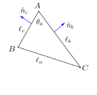
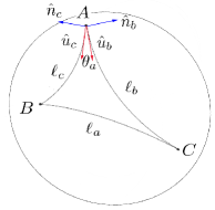
Figure 1: The hyperbolic triangle is represented in the Poincaré disc. The (outgoing) normals $\hat{n}_{i}$ are defined in the tangent plane at the vertex of the triangle, as the orthogonal vectors to the tangent vectors $\hat{u}_{i}$.

Let us consider now an hyperbolic triangle. Its edges are geodesics in the 2d hyperboloid of radius $R$. Unlike the flat triangle, an hyperbolic triangle can be characterized by its three angles $\theta_{i}$ or the three lengths $\ell_{i}$ of its edges. The hyperbolic cosine laws relate the edge lengths and the angles (see the table below). The area ${\mathcal{A}}$ of the triangle is given in terms of the angles.

$${\mathcal{A}}=(\pi-(\theta_{a}+\theta_{b}+\theta_{c}))R^{2}.$$ (178)

In order to make easier the limit to the flat case, we can encode all this information in terms of the normals. Note however that due to the curvature, we have a different tangent space at each point of the edge. The tangent vectors and their normal are therefore not living in the same vector space for different points. In the curved case, we shall consider the normals $\vec{n}_{i}$ at each vertex of the triangle. As a direct consequence, the closure constraint in the curved case is subtler than in the flat case. We postpone the study of this constraint to a detailed analysis of the relevant phase space in phase space . We recall in the following table the main geometric features of the flat and hyperbolic triangles, in terms of the normals. We use the notation $s=\frac{1}{2}(\ell_{a}+\ell_{b}+\ell_{c})$.

	Flat case, $\Lambda=0$	Hyperbolic case, $\Lambda<0$, $R=|\Lambda|^{-\frac{1}{2}}$
Closure constraint:	$\sum_{i}\vec{n}_{i}=0$	To be determined phase space
Edge length:	$|\vec{n}_{i}|=\ell_{i}$	$|\vec{n}_{i}|=\sinh\frac{\ell_{i}}{R}$
Cosine law:	$\cos\theta_{a}=-\hat{n}_{b}\cdot\hat{n}_{c}=-\frac{\ell_{a}^{2}-\ell_{b}^{2}-\ell_{c}^{2}}{2\ell_{b}\ell_{c}}$	$\cos\theta_{a}=-\hat{n}_{b}\cdot\hat{n}_{c}=\frac{-\cosh\frac{\ell_{a}}{R}+\cosh\frac{\ell_{b}}{R}\cosh\frac{\ell_{c}}{R}}{\sinh\frac{\ell_{b}}{R}\sinh\frac{\ell_{c}}{R}}$
Area:	${\mathcal{A}}^{2}=\frac{1}{4}\left(s(s-\ell_{a})(s-\ell_{b})(s-\ell_{c})\right)$	$\sin^{2}\frac{{\mathcal{A}}}{2R^{2}}=\frac{\sinh(\frac{s}{2R})\sinh(\frac{s-\ell_{a}}{2R})\sinh(\frac{s-\ell_{b}}{2R})\sinh(\frac{s-\ell_{c}}{2R})}{\cosh^{2}\frac{\ell_{a}}{2R}\cosh^{2}\frac{\ell_{b}}{2R}\cosh^{2}\frac{\ell_{c}}{2R}}$

The quantization of the flat triangle can be done very naturally. The quantum state is given by the three-leg $\mathrm{SU}(2)$ intertwiner. We associate to normalized normals $\vec{n}_{i}$ to the flux operators $\,{}^{(i)}\vec{J}$, which we know now to be related to the $\mathrm{SU}(2)$ vector operators $\,{}^{(i)}\tau^{1}$ (cf section III.2). This provides a direct quantization of all the geometric data: closure constraint, length, angles, area (see valentin-laurent for a recent review of these results).

We consider now a ${{\mathcal{U}}_{q}({\mathfrak{s}u}(2))}$ three-leg intertwiner $|\iota_{j_{b}j_{c}j_{a}}\rangle$. The ordering we choose for the legs is fixed as we have already emphasized before. We would like to check whether it encodes the quantum state of an hyperbolic triangle. We use the ${{\mathcal{U}}_{q}({\mathfrak{s}u}(2))}$ tensor operators to probe the geometry of this state of geometry. Since we are in the 3d framework with a negative cosmological constant, we take $q=e^{\lambda}$, with $\lambda=\frac{\ell_{p}}{R}$, and $\Lambda=-R^{2}$.

Angle operator.

Since we know that the angles specify completely the hyperbolic triangle, we can focus first on operators characterizing angles. By analogy with the non-deformed case, we define the scalar product of the vector operators $\,{}^{(i)}\hat{\bf t}^{1}$ and $\,{}^{(j)}\hat{\bf t}^{1}$, with chosen normalization $\hat{N}^{1}_{j_{i}}=1$ and $i\neq j$. We look at the action of this operator on the three-leg intertwiner $|\iota_{j_{b}j_{c}j_{a}}\rangle$. For simplicity we focus on $\,{}^{(b)}\hat{\bf t}^{1}\cdot\,^{(c)}\hat{\bf t}^{1}$, since we know how to recover the other types of operators from this one using tricks developed in Section IV.1.

$$\,{}^{(b)}\hat{\bf t}^{1}\cdot\,^{(c)}\hat{\bf t}^{1}\,|\iota_{j_{b}j_{c}j_{a}}\rangle = -q\,\frac{\cosh\frac{\lambda}{2}\cosh((j_{a}+\frac{1}{2})\lambda)-\cosh((j_{b}+\frac{1}{2})\lambda)\cosh((j_{c}+\frac{1}{2})\lambda))}{\sqrt{(\sinh(j_{b}\lambda))(\sinh((j_{b}+1)\lambda))(\sinh(j_{c}\lambda))(\sinh((j_{c}+1)\lambda))}}|\iota_{j_{b}j_{c}j_{a}}\rangle,$$ (179)

$$= -q\,\frac{\cosh\frac{\lambda}{2}\cosh((j_{a}+\frac{1}{2})\lambda)-\cosh((j_{b}+\frac{1}{2})\lambda)\cosh((j_{c}+\frac{1}{2})\lambda))}{\sqrt{(\sinh^{2}((j_{b}+\frac{1}{2})\lambda)-\sinh^{2}\frac{\lambda}{2})(\sinh^{2}((j_{c}+\frac{1}{2})\lambda)-\sinh^{2}\frac{\lambda}{2})}}|\iota_{j_{b}j_{c}j_{a}}\rangle,$$

where we have used $q=e^{\lambda}$ and $\sinh(j\lambda))(\sinh((j+1)\lambda))=\sinh^{2}((j+\frac{1}{2})\lambda)-\sinh^{2}\frac{\lambda}{2}$. We recognize in (179) a quantization of the hyperbolic cosine law, provided we consider the quantization of the length edge given by $\ell\rightarrow(j+\frac{1}{2})\ell_{p}$. Note that the factors $\sinh^{2}\frac{\lambda}{2}$ in the denominator and $\cosh\frac{\lambda}{2}$ in the numerator can be interpreted as ordering ambiguity factors, arising from the respective quantization of $\sinh\frac{\ell_{i}}{R}$ and $\cosh\frac{\ell_{i}}{R}$.

In the limit $q\rightarrow 1$, we recover the quantized cosine law for a flat triangle seth expressed in terms of the quantized normals, modulo an overall sign and a factor $\frac{1}{2}$.

$$\,{}^{(b)}\hat{\tau}^{1}\cdot\,^{(c)}\hat{\tau}^{1}\,|\iota_{j_{a}j_{b}j_{c}}\rangle = -\left(\frac{j_{a}(j_{a}+1)-j_{b}(j_{b}+1)-j_{c}(j_{c}+1)}{\sqrt{j_{b}(j_{b}+1)j_{c}(j_{c}+1)}}+{\mathcal{O}}\left(\lambda^{2}\right)\right)\,|\iota_{j_{b}j_{c}j_{a}}\rangle.$$ (180)

From the construction of the vector operators, in section III.2, we know that

$$\,{}^{(b)}\hat{\tau}^{1}\cdot\,^{(c)}\hat{\tau}^{1}|\iota_{j_{a}j_{b}j_{c}}\rangle=-\frac{2}{\sqrt{j_{b}(j_{b}+1)j_{c}(j_{c}+1)}}\,^{(b)}\vec{J}\cdot\,^{(c)}\vec{J}\,|\iota_{j_{a}j_{b}j_{c}}\rangle.$$

This allows to identify the source of the discrepancy for the $\frac{1}{2}$ and the overall sign. In particular, the global minus sign in (179) and (180) with respect to the flat/hyperbolic cosine law comes simply from the definition of the scalar product we have used.

Since $\,{}^{(i)}\vec{J}$ is interpreted in the LQG formalism as the quantized normal to the edge of the triangle, in the deformed case, we interpret $\,{}^{(b)}\hat{\bf t}^{1}$ and $\,{}^{(c)}\hat{\bf t}^{1}$ as the quantized normals respectively of the edges $AC$ and $AB$, at the vertex $A$ of the hyperbolic triangle.

We can play with the normalization of the vector operators to have a better defined hyperbolic law. Indeed, we notice that both (179) and (180) diverge when $j=0$. Instead of taking the vector operator $\,{}^{(i)}\hat{\bf t}^{1}$ with normalization $N^{1}_{j_{i}}=1$, we can consider $\,{}^{(i)}\tilde{\bf t}^{1}$ with normalization

$$\tilde{N}^{1}_{j}\equiv\frac{\sqrt{\sinh(j\lambda)\,\sinh((j+1)\lambda)}}{\sinh((j+\frac{1}{2})\lambda)}\stackrel{{\scriptstyle q\rightarrow 1}}{{\rightarrow}}\frac{\sqrt{j(j+1)}}{j+\frac{1}{2}}.$$ (181)

In this case the cosine laws become well behaved for small $j$.

$$\,{}^{(b)}\tilde{\bf t}^{1}\cdot\,^{(c)}\tilde{\bf t}^{1}\,|\iota_{j_{b}j_{c}j_{a}}\rangle=q\,\frac{\cosh\frac{\ell_{p}}{2\ell_{c}}\cosh((j_{a}+\frac{1}{2})\lambda)-\cosh((j_{b}+\frac{1}{2})\lambda)\cosh((j_{c}+\frac{1}{2})\lambda))}{{\sinh((j_{b}+\frac{1}{2})\lambda)\,\sinh((j_{c}+\frac{1}{2})\lambda)}}|\iota_{j_{b}j_{c}j_{a}}\rangle.$$ (182)

When dealing with a non-zero cosmological constant and the Planck length, by dimensional analysis, one can expect to have a minimum angle eugenio . This can now be explicitly checked. Setting $j_{a}=0$, we must have $j_{b}=j_{c}=j$ since we deal with an intertwiner, and the quantum cosine law (179) gives

$$\theta_{a}^{min}(j)=\arccos\left(q\frac{\cosh^{2}\frac{\lambda}{2}-\cosh^{2}((j+\frac{1}{2})\lambda)}{{\sinh^{2}((j+\frac{1}{2})\lambda)-\sinh^{2}\frac{\lambda}{2}}}\right),$$ (183)

which means that there is a non-zero minimum angle. When $\ell_{p}\rightarrow 0$ (classical limit) or $R\rightarrow\infty$ (flat quantum limit), (183) tends to 1, so we recover that the triangle is degenerated.

As expected, the angle observables can be expressed in terms of the ${{\mathcal{U}}_{q}({\mathfrak{s}u}(2))}$ generators.

$$i>j,\,\,^{(i)}\hat{\bf t}^{1}\cdot\,^{(j)}\hat{\bf t}^{1}=\left(q^{-\frac{3}{2}}(-{\mathcal{E}}_{ij}{\mathcal{E}}_{ji}+{\mathcal{E}}_{ii})+\frac{1}{[2]}{\mathcal{E}}_{ii}{\mathcal{E}}_{jj}\right),\quad i<j,\,\,^{(i)}\hat{\bf t}^{1}\cdot\,^{(j)}\hat{\bf t}^{1}=\left(q^{\frac{1}{2}}(-{\mathcal{E}}_{ij}{\mathcal{E}}_{ji}+{\mathcal{E}}_{ii})+\frac{q^{2}}{[2]}{\mathcal{E}}_{ii}{\mathcal{E}}_{jj}\right).$$

Length operator.

The length operator is obtained by looking at the norm of the unnormalized vector operator $\,{}^{(i)}{\bf t}^{1}$ with normalization $N^{i}_{j}$.

$${}^{(i)}{\bf t}^{1}\cdot^{(i)}{\bf t}^{1}|\iota_{j_{b}j_{c}j_{a}}\rangle=\left(N^{1}_{j_{i}}\right)^{2}|\iota_{j_{b}j_{c}j_{a}}\rangle,\quad i=a,b,c.$$ (184)

Keeping in mind that $\,{}^{(i)}{\bf t}^{1}$ encodes the quantization of the normal, by inspection of the classical and quantum hyperbolic cosine law, it is natural to take

$$N^{1}_{j}=\sqrt{\sinh^{2}((j+\frac{1}{2})\lambda)-\sinh^{2}(\frac{\lambda}{2})}\textrm{ or }\tilde{\bf N}^{1}_{j}=\sinh((j+\frac{1}{2})\lambda).$$ (185)

The normalization $\tilde{\bf N}^{1}_{j}$ leads to the regularized hyperbolic cosine law (182). We note therefore that the norm of the vector operator corresponds to a function of the length operator. The length is quantized, with eigenvalue $(j+\frac{1}{2})\ell_{p}$ as we have argued previously. The norm of the vector operator can be expressed in terms of the ${\mathcal{E}}$ operators.

$$\,{}^{(i)}{\bf t}^{1}\cdot\,^{(i)}{\bf t}^{1}=\frac{1}{[2]}(-q{\mathcal{E}}^{2}_{i}-(1+q^{{-1}}){\mathcal{E}}_{i}).$$ (186)

”Area” operator.

In the flat case, one expresses the square of the area of the triangle in terms of a cosine and the norm of the normals so that the operator is easy to quantize, using vector operators area-etera .

$${\mathcal{A}}^{2}=\frac{1}{4}\left(|\vec{n}_{b}|^{2}|\vec{n}_{c}|^{2}-(\vec{n}_{c}\cdot\vec{n}_{c})^{2}\right)$$ (187)

We proceed in the same manner in the hyperbolic case. We do not consider the square of the area but instead the square of the sine of the area. Indeed, the area of an hyperbolic triangle is given in terms of the triangle angles (178). There are various ways to express functions of the area in terms of the edge lengths mend . A convenient one will be

$$\sin^{2}\frac{{\mathcal{A}}}{2R^{2}}=\frac{\sinh(\frac{s}{2R})\sinh(\frac{s-\ell_{a}}{2R})\sinh(\frac{s-\ell_{b}}{2R})\sinh(\frac{s-\ell_{c}}{2R})}{\cosh^{2}\frac{\ell_{a}}{2R}\cosh^{2}\frac{\ell_{b}}{2R}\cosh^{2}\frac{\ell_{c}}{2R}},$$ (188)

where $s=\frac{1}{2}(\ell_{a}+\ell_{b}+\ell_{c})$. Of course, in the flat limit, $R\rightarrow\infty$, we recover Heron’s formula (see the above table).

Playing with the cosine laws, we can express $\sin^{2}\frac{{\mathcal{A}}}{2R^{2}}$ only in terms of the normals.

$$\sin^{2}\frac{{\mathcal{A}}}{2R^{2}}=\frac{1}{4}\frac{\sinh^{2}\frac{\ell_{b}}{R}\sinh^{2}\frac{\ell_{c}}{R}(1-\cos^{2}\theta_{a})}{(\cosh^{2}\frac{\ell_{a}}{2R}\cosh^{2}\frac{\ell_{b}}{2R}\cosh^{2}\frac{\ell_{c}}{2R})}=2\frac{|\vec{n}_{b}|^{2}|\vec{n}_{c}|^{2}-(\vec{n}_{b}\cdot\vec{n}_{c})^{2}}{(1+\sqrt{1+|\vec{n}_{a}|^{2}})(1+\sqrt{1+|\vec{n}_{b}|^{2}})(1+\sqrt{1+|\vec{n}_{c}|^{2}})}.$$ (189)

There is no difficulty in quantizing this expression since it only involves scalar products and norms of nromals, which upon quantization become operators that are diagonal and functions of the Casimir operator. There is therefore no ordering issue anywhere. The area has also a discrete spectrum.

Outlook

Summary:

Let us summarize the main results of our paper. We have recalled the definition of tensor operators for ${{\mathcal{U}}_{q}({\mathfrak{s}u}(2))}$, with q real, which is the relevant case to study Euclidian 3d LQG with $\Lambda<0$ and Lorentzian 3+1 LQG with $\Lambda>0$.

We have shown how they are the natural objects to construct observables for a ${{\mathcal{U}}_{q}({\mathfrak{s}u}(2))}$ intertwiner. These operators are the key to study LQG defined in terms of a quantum group as they provide sets of operators that transform well under the quantum group. We have generalized the $U(n)$ formalism to the quantum group ${{\mathcal{U}}_{q}({\mathfrak{s}u}(2))}$. That is, we have shown how we can construct a closed algebra of observables (i.e.  invariant under ${{\mathcal{U}}_{q}({\mathfrak{s}u}(2))}$) which can be related to the quantum group ${{\mathcal{U}}_{q}({\mathfrak{u}}(n))}$. This means that the ${{\mathcal{U}}_{q}({\mathfrak{s}u}(2))}$ intertwiner carries a ${{\mathcal{U}}_{q}({\mathfrak{u}}(n))}$ representation, which we argued must be irreducible. We have constructed the natural generalization of the LQG geometric operators and interpreted them in the 3d Euclidian setting. We have shown that a three-leg ${{\mathcal{U}}_{q}({\mathfrak{s}u}(2))}$ intertwiner encodes the quantum state of an hyperbolic triangle. We have also shown how the presence of a cosmological constant leads to a notion of minimum angle as expected eugenio . These results provide new evidences for the use of quantum group as a tool to encode the cosmological constant, in the LQG formalism.

Note that the use of tensor operators can be also useful for dealing with lattice Yang-Mills theories built with ${{\mathcal{U}}_{q}({\mathfrak{s}u}(2))}$ as gauge group. In particular it could be interesting to see how tensor operators can be useful to implement observables in the recent work bianca . In fact, there are a number of interesting routes open for exploration.

Hyperbolic polyhedra:

We have studied the geometric operators in the context of 3d LQG. We have shown that they induce a quantum hyperbolic geometry. These operators should also be interpreted in the 3+1 LQG case. The vector operator acting on a leg $i$ would be interpreted as the quantization of the normal of the $i^{th}$ face of the polyhedron. The squared norm of the vector operator acting on each leg would be now interpreted as a function of the squared area operator. This implies that in this case we still expect to have a discrete spectrum for the (squared) area. The angle operator would now encode the quantization of the dihedral angle, the angle between normals. One could then construct the analogue of the squared volume operator, using the triple product between vector operators. Following the intuition gained from looking at the area operator for the triangle, we would then expect to get an expression of a function of the volume of the hyperbolic polyhedron. We leave for further investigations the properties of such operator, as well as other interesting geometric operators we could construct to probe the quantum geometry of hyperbolic polyhedra.

Phase space structure:

One of our key results is that the quantum group spin networks can be used in the LQG context to introduce the cosmological constant. Recent developments have shown that spin networks can be seen as quantum states of flat discrete geometries, when $\Lambda=0$. The phase space structure is nicely described in the ”twisted geometries” framework. Since we have identified the meaning of the quantum geometric operators, built from the vector operators, this can provide some guiding lines in identifying the relevant phase space structure, i.e.  the notion of curved twisted geometries. In particular, one knows that the classical analogue of a quantum group is a Poisson-Lie group, so we can expect to use this structure to define the curved twisted geometries. This is work in progress phase space .

Other signatures and other signs for $\Lambda$:

When defining tensor operators, we have focused on ${{\mathcal{U}}_{q}({\mathfrak{s}u}(2))}$ with $q$ real. This choice provided the relevant structure to study the physical case, 3+1 LQG with $\Lambda>0$. However, there is a number of other cases to study. At the classical level, with $q=1$, we could explore the construction of tensor operators for $\mathrm{SL}(2,{\mathbb{R}})$, which would be relevant for Lorentzian 2+1 LQG with $\Lambda=0$. Interestingly, the Wigner-Eckart theorem has not been defined for $\mathrm{SL}(2,{\mathbb{R}})$, that is there is no general formula for tensor operators transforming as $\mathrm{SL}(2,{\mathbb{R}})$ (non-unitary) finite dimensional and discrete representations. This is work in progress lorentzian . It would be then relevant to discuss the quantum group version of this structure, which would be relevant for 2+1 Lorentzian gravity with $\Lambda\neq 0$.

Another interesting case to explore would be ${{\mathcal{U}}_{q}({\mathfrak{s}u}(2))}$ with $q$ root of unity, which would be relevant for 3d Euclidan LQG with $\Lambda>0$. We have not considered this case here as ${{\mathcal{U}}_{q}({\mathfrak{s}u}(2))}$ with $q$ root of unity is not a quasi-triangular Hopf algebra, but a quasi-Hopf algebra. This means that the construction in rittenberg does not apply directly. On the other hand, the representation theory of ${{\mathcal{U}}_{q}({\mathfrak{s}u}(2))}$ with $q$ root of unity can be trimmed of the unwanted features so that its recoupling theory can be well under control chari . This is why the Turaev Viro model can still be defined as it is. It is then quite likely that we can define the tensor operators in this case, in terms of their matrix elements, which would be proportional to the Clebsh-Gordan coefficients. We leave this for further investigations.

Hamiltonian constraint:

LQG and spinfoams are supposed to be the two facets of the same theory. This can be shown explicitly only in the case $\Lambda=0$ case, in 3d ale-karim . Recently, an Hamiltonian constraint was constructed using the spinor formalism valentin-etera . It has been designed to encode a recursion relation on the $6j$ symbol and hence by construction, it relates the Ponzano-Regge model to the LQG approach. Now that we have generalized the spinor approach to the quantum group case, we can construct a $q$-deformed version of this Hamiltonian constraint. It would essentially encode the recursion relation of the $q$-deformed $6j$ symbol. Hence this new $q$-deformed Hamiltonian constraint would relate the Turaev-Viro model and LQG with a cosmological constant. This is work in progress hamiltonian .

Aknowledgements: We would like to thank A. Baratin, V. Bonzom, B. Dittrich, L. Freidel, E. Livine for many interesting discussions and comments.

Appendix A Hyperbolic cosine law

Consider the upper 2d hyperboloid $H_{+}^{2}$, embedded into ${\mathbb{R}}^{3}$, with curvature $-R^{-2}=\Lambda$, where $R$ is the radius of curvature.

$$H_{+}^{2} = \{\vec{x}\in{\mathbb{R}}^{3},\;x_{1}>0,\,x_{i}\eta^{ij}x_{j}=x_{1}^{2}-x_{2}^{2}-x_{3}^{2}=|\vec{x}|^{2}=R^{2}\}.$$ (190)

On $H_{+}^{2}$, consider three points $A,B,C$ and the geodesics joining them: we obtain an hyperbolic triangle. Without loss of generality, we can always assume that $A$ sits at the origin of $H_{+}^{2}$, that is as a point of ${\mathbb{R}}^{3}$, it is given by the vector $\vec{A}=(R,0,0)$. The points $B$ and $C$ are then obtained from $\vec{A}$ by performing a boost $L_{c},\,L_{b}$ with respective rapidity $c$ and $b$. Explicitly,

$$\vec{B}=L_{c}\vec{A},\quad\vec{C}=L_{b}\vec{A}.$$ (191)

As a consequence, we have $\langle\vec{A},\vec{A}\rangle=|\vec{A}|^{2}=|\vec{B}|^{2}=|\vec{C}|^{2}=R^{2}$.

Consider the normalized space-like vectors $\hat{u}_{AB},\,\hat{u}_{AC}\in T_{A}H_{+}^{2}$, the tangent plane of $H_{+}^{2}$ at the point $A$. They are the tangent vectors to the geodesics joining respectively $A$ to $B$ and $A$ to $C$. By construction, these vectors are orthogonal to $\vec{A}$.

$$\hat{u}_{AB}=\frac{\vec{B}-\frac{1}{R^{2}}\langle\vec{A},\vec{B}\rangle\vec{A}}{\left|\vec{B}-\frac{1}{R^{2}}\langle\vec{A},\vec{B}\rangle\vec{A}\right|}, \hat{u}_{AC}=\frac{\vec{C}-\frac{1}{R^{2}}\langle\vec{A},\vec{C}\rangle\vec{A}}{\left|\vec{C}-\frac{1}{R^{2}}\langle\vec{A},\vec{C}\rangle\vec{A}\right|}$$ (192)

Since we are dealing with an homogeneous space, we express the lengths $\ell_{i}$ of the geodesic arcs using the dimensionful parameter $R$, such that $\ell_{c}=Rc$, $\ell_{b}=Rb$ as well as $\ell_{a}=Ra$.

By definition, we know that the angle between two geodesics which intersect is defined in terms of the angle between the tangent vectors. If we focus in particular on the angle $\alpha$ between the arcs $AB$ and $AC$, we have

$$\cos\alpha=\langle\hat{u}_{AB},\hat{u}_{AC}\rangle.$$ (193)

Using the expression of the tangent vectors, we obtain the hyperbolic cosine law.

$$\cos\alpha = \frac{-\cosh\frac{\ell_{a}}{R}+\cosh\frac{\ell_{b}}{R}\cosh\frac{\ell_{c}}{R}}{\sinh\frac{\ell_{b}}{R}\sinh\frac{\ell_{c}}{R}}$$ (194)

In the flat case, performing the limit $R\rightarrow\infty$ in (194), we recover the al Khashi rule

$$\cos\alpha=\frac{-\ell_{a}^{2}+(\ell_{b}^{2}+\ell_{c}^{2})}{2\ell_{b}\ell_{c}}.$$ (195)

Appendix B Useful formulae

These formulae are taken from the book BiedenharnBook .

$q$-Clebsch-Gordan

An explicit expression of the $q$-Clebsch-Gordan in the van der Waerden form is given as

$$\,{}_{q}\textbf{C}\begin{array}[]{c@{}c@{}c}j_{1}&j_{2}&j\\ m_{1}&m_{2}&m\end{array} := \delta_{m,m_{1}+m_{2}}q^{\frac{1}{4}(j_{1}+j_{2}-j)(j_{1}+j_{2}+j+1)+\frac{1}{2}(j_{1}m_{2}-j_{2}m_{1})}\Delta(j_{1}j_{2}j)$$ (198)

$$\times \left([j_{1}+m_{1}]![j_{1}-m_{1}]![j_{2}+m_{2}]![j_{2}-m_{2}]![j+m]![j-m]![2j+1]\right)^{\frac{1}{2}}$$ (199)

$$\times \sum_{n}\frac{(-1)^{n}q^{-\frac{n}{2}(j_{1}+j_{2}+j+1)}}{[n]![j_{1}+j_{2}-j-n]![j_{1}-m_{1}-n]![j_{2}+m_{2}-n]![j-j_{2}+m_{1}+n]![j-j_{1}-m_{2}+n]!}.$$ (200)

where the triangle function $\Delta$ is given by

$$\Delta(abc):=\left(\frac{[a+b-c]![a-b+c]![-a+b+c]!}{[a+b+c+1]!}\right)^{\frac{1}{2}}.$$ (201)

For $q\rightarrow 1$ the $q$-Clebsch-Gordan coefficients reduce to the usual CG coefficients in the van der Waerden form.

The $q$-Clebsch-Gordan coefficients have two orthogonality relations.

$$\sum_{m_{1},m_{2}}\,{}_{q}\textbf{C}\begin{array}[]{c@{}c@{}c}j_{1}&j_{2}&j\\ m_{1}&m_{2}&m\end{array}\,_{q}\textbf{C}\begin{array}[]{c@{}c@{}c}j_{1}&j_{2}&j^{\prime}\\ m_{1}&m_{2}&m^{\prime}\end{array} = \delta_{jj^{\prime}}\delta_{mm^{\prime}}$$ (206)

$$\sum_{j,m}\,{}_{q}\textbf{C}\begin{array}[]{c@{}c@{}c}j_{1}&j_{2}&j\\ m_{1}&m_{2}&m\end{array}\,_{q}\textbf{C}\begin{array}[]{c@{}c@{}c}j_{1}&j_{2}&j\\ m^{\prime}_{1}&m^{\prime}_{2}&m\end{array} = \delta_{m_{1}m^{\prime}_{1}}\delta_{m_{2}m^{\prime}_{2}}.$$ (211)

Note that in the first equation, we have assumed that $j_{1},j_{2}$ and $j$ satisfy the triangle conditions.

The $q$-Clebsch-Gordan coefficients have some symmetries. We list the most relevant ones for our concerns.

$$\,{}_{q}\textbf{C}\begin{array}[]{c@{}c@{}c}j_{1}&j_{2}&j\\ m_{1}&m_{2}&m\end{array} = (-1)^{j_{1}+j_{2}-j}\,_{q^{{-1}}}\textbf{C}\begin{array}[]{c@{}c@{}c}j_{1}&j_{2}&j\\ -m_{1}&-m_{2}&-m\end{array}$$ (216)

$$\,{}_{q}\textbf{C}\begin{array}[]{c@{}c@{}c}j_{1}&j_{2}&j\\ m_{1}&m_{2}&m\end{array} = (-1)^{j_{1}+j_{2}-j}\,_{q^{{-1}}}\textbf{C}\begin{array}[]{c@{}c@{}c}j_{2}&j_{1}&j\\ m_{2}&m_{1}&m\end{array}$$ (221)

$$\,{}_{q}\textbf{C}\begin{array}[]{c@{}c@{}c}j_{1}&j_{2}&j\\ m_{1}&m_{2}&m\end{array} = (-1)^{j-j_{2}-m_{1}}q^{\frac{m_{1}}{2}}\sqrt{\frac{[2j+1]}{[2j_{2}+1]}}\,_{q}\textbf{C}\begin{array}[]{c@{}c@{}c}j_{1}&j&j_{2}\\ -m_{1}&m&m_{2}\end{array}.$$ (226)

The value of some specific CG coefficients.

$$\,_{q}\textbf{C}\begin{array}[]{c@{}c@{}c}j_{1}&j_{2}&0\\ m_{1}&m_{2}&0\end{array}=\delta_{j_{1},j_{2}}\,\delta_{m_{1},-m_{2}}\,\frac{(-1)^{j_{1}-m_{1}}q^{\frac{m_{1}}{2}}}{\sqrt{[2j_{1}+1]}}.$$ (227)

$$\,{}_{q}\textbf{C}\begin{array}[]{c@{}c@{}c}1&1&1\\ 1&0&1\end{array}=q^{1/2}\sqrt{\frac{[2]}{[4]}},\quad\,_{q}\textbf{C}\begin{array}[]{c@{}c@{}c}1&1&1\\ 0&1&1\end{array}=-q^{-1/2}\sqrt{\frac{[2]}{[4]}},\quad\,_{q}\textbf{C}\begin{array}[]{c@{}c@{}c}1&1&1\\ -1&0&-1\end{array}=-q^{-1/2}\sqrt{\frac{[2]}{[4]}},\quad\,_{q}\textbf{C}\begin{array}[]{c@{}c@{}c}1&1&1\\ 0&-1&-1\end{array}=q^{1/2}\sqrt{\frac{[2]}{[4]}},$$ (236)

$$\,{}_{q}\textbf{C}\begin{array}[]{c@{}c@{}c}1&1&1\\ 1&-1&0\end{array}=\sqrt{\frac{[2]}{[4]}},\quad\,_{q}\textbf{C}\begin{array}[]{c@{}c@{}c}1&1&1\\ -1&1&0\end{array}=-\sqrt{\frac{[2]}{[4]}},\quad\,_{q}\textbf{C}\begin{array}[]{c@{}c@{}c}1&1&1\\ 0&0&0\end{array}=\sqrt{\frac{[2]}{[4]}}\left(q^{\frac{1}{2}}-q^{-\frac{1}{2}}\right).$$ (243)

$q$-$6j$-symbol

The q-$6j$-symbol is invariant under the rescaling $q\rightarrow q^{{-1}}$. It satisfies the following orthogonality relation.

$$\sum_{j}\,\left\{\begin{array}[]{ccc}b&c&j\\ k&a&n\end{array}\right\}\,\,\left\{\begin{array}[]{ccc}a&b&m\\ c&k&j\end{array}\right\}\, = \delta_{mn}$$ (248)

The contraction of two q-$6j$-symbol can give another one. This is a useful property for us.

$$\sum_{m}(-1)^{a+b+c+k-j-m-n}q^{\frac{1}{2}(a(a+1)+b(b+1)+c(c+1)+k(k+1)-j(j+1)-m(m+1)-n(n+1))}\,\left\{\begin{array}[]{ccc}a&b&m\\ c&k&j\end{array}\right\}\,\,\left\{\begin{array}[]{ccc}a&c&n\\ k&b&m\end{array}\right\}\, = \,\left\{\begin{array}[]{ccc}a&c&n\\ b&k&j\end{array}\right\}\,$$ (255)

It has some symmetries when moving some of its elements.

$$\,\left\{\begin{array}[]{ccc}a&b&m\\ c&k&j\end{array}\right\}\,=\,\left\{\begin{array}[]{ccc}c&k&m\\ a&b&j\end{array}\right\}\,$$ (260)

A specific value of the q-$6j$-symbol which is relevant to us is

$$\,\left\{\begin{array}[]{ccc}j_{1}&j_{1}&1\\ j_{2}&j_{2}&j_{3}\end{array}\right\}\, = (-1)^{j_{1}+j_{2}+j_{3}}\frac{[j_{2}+j_{3}-j_{1}][j_{1}+j_{3}-j_{2}]-[j_{1}+j_{2}-j_{3}][j_{1}+j_{2}+j_{3}+2]}{\left([2j_{1}][2j_{1}+1][2j_{1}+2][2j_{2}][2j_{2}+1][2j_{2}+2]\right)^{\frac{1}{2}}}.$$ (263)

$$\,_{q}\textbf{C}\begin{array}[]{c@{}c@{}c}\frac{1}{2}&\frac{1}{2}&1\\ \frac{1}{2}&\frac{1}{2}&1\end{array}=1=\,\,_{q}\textbf{C}\begin{array}[]{c@{}c@{}c}\frac{1}{2}&\frac{1}{2}&1\\ -\frac{1}{2}&-\frac{1}{2}&-1\end{array},\quad\,_{q}\textbf{C}\begin{array}[]{c@{}c@{}c}\frac{1}{2}&\frac{1}{2}&1\\ \frac{1}{2}&-\frac{1}{2}&0\end{array}=\frac{q^{-\frac{1}{4}}}{\sqrt{[2]}},\quad\,_{q}\textbf{C}\begin{array}[]{c@{}c@{}c}\frac{1}{2}&\frac{1}{2}&1\\ -\frac{1}{2}&\frac{1}{2}&0\end{array}=\frac{q^{\frac{1}{4}}}{\sqrt{[2]}},$$ (264)

${\mathcal{R}}$-matrix and deformed permutation

The ${\mathcal{R}}$-matrix for ${{\mathcal{U}}_{q}({\mathfrak{s}u}(2))}$ can be expressed in terms of the $q$-Clebsch-Gordan .

$$\left({\mathcal{R}}^{j_{1}j_{2}}\right)^{m_{1}m_{2}}_{m^{\prime}_{1}m^{\prime}_{2}} = \sum_{j,m}q^{-\frac{1}{2}\left(j_{1}(j_{1}+1)+j_{2}(j_{2}+1)-j(j+1)\right)}\,_{q}\textbf{C}\begin{array}[]{ccc}j_{1}&j_{2}&j\\ m_{1}&m_{2}&m\end{array}\;\,_{q^{{-1}}}\textbf{C}\begin{array}[]{ccc}j_{1}&j_{2}&j\\ m^{\prime}_{1}&m^{\prime}_{2}&m\end{array}$$ (269)

$$= \sum_{j,m}(-1)^{j_{1}+j_{2}-j}\,q^{-\frac{1}{2}\left(j_{1}(j_{1}+1)+j_{2}(j_{2}+1)-j(j+1)\right)}\,_{q}\textbf{C}\begin{array}[]{ccc}j_{1}&j_{2}&j\\ m_{1}&m_{2}&m\end{array}\;\,_{q}\textbf{C}\begin{array}[]{ccc}j_{2}&j_{1}&j\\ m^{\prime}_{2}&m^{\prime}_{1}&m\end{array},$$ (274)

with $m_{1}+m_{2}=m^{\prime}_{1}+m^{\prime}_{2}$ and $m^{\prime}_{1}-m_{1}\geq 0$ (this is zero otherwise). The second equation has been obtained using the symmetries of the $q$-Clebsch-Gordan coefficients.

The inverse of the ${\mathcal{R}}$-matrix is obtained from the above formulae by setting $q\rightarrow q^{{-1}}$.

$$\left({{\mathcal{R}}^{-1}}^{j_{1}j_{2}}\right)^{m_{1}m_{2}}_{m^{\prime}_{1}m^{\prime}_{2}} = \sum_{j,m}(-1)^{j_{1}+j_{2}-j}\,q^{\frac{1}{2}\left(j_{1}(j_{1}+1)+j_{2}(j_{2}+1)-j(j+1)\right)}\,_{q^{{-1}}}\textbf{C}\begin{array}[]{ccc}j_{1}&j_{2}&j\\ m_{1}&m_{2}&m\end{array}\;\,_{q^{{-1}}}\textbf{C}\begin{array}[]{ccc}j_{2}&j_{1}&j\\ m^{\prime}_{2}&m^{\prime}_{1}&m\end{array}$$ (279)

$$= \sum_{j,m}(-1)^{j_{1}+j_{2}-j}\,q^{\frac{1}{2}\left(j_{1}(j_{1}+1)+j_{2}(j_{2}+1)-j(j+1)\right)}\,_{q}\textbf{C}\begin{array}[]{ccc}j_{2}&j_{1}&j\\ m_{2}&m_{1}&m\end{array}\;\,_{q}\textbf{C}\begin{array}[]{ccc}j_{1}&j_{2}&j\\ m^{\prime}_{1}&m^{\prime}_{2}&m\end{array}$$ (284)

One can check that this is true by evaluating ${\mathcal{R}}^{{-1}}{\mathcal{R}}$ and use the orthogonality properties of the $q$-Clebsch-Gordan coefficients. Furthermore we can check that when $q\rightarrow 1$, we recover that the ${\mathcal{R}}$-matrix is simply the identity map (for this one uses the classical version of (221) and the orthogonality relation (211)).

We are interested in the deformed permutation $\psi_{\mathcal{R}}=\psi{\mathcal{R}}$ (resp. $\psi_{\mathcal{R}}^{{-1}}={\mathcal{R}}^{{-1}}\psi$), which means that instead of considering ${{\mathcal{R}}}^{j_{1}j_{2}}$ (resp. ${{\mathcal{R}}^{-1}}^{j_{1}j_{2}}$), we consider ${{\mathcal{R}}}^{j_{2}j_{1}}$ (resp. ${{\mathcal{R}}^{-1}}^{j_{2}j_{1}}$). The relevant formula for ${{\mathcal{R}}}^{j_{2}j_{1}}$ is obtained from (274) by exchanging $j_{1}$ and $j_{2}$.

References

- (1) S. Finazzi, S. Liberati and L. Sindoni, Cosmological Constant: A Lesson from Bose-Einstein Condensates, Phys. Rev. Lett. 108 (2012) 071101 [arXiv:1103.4841 [gr-qc]].
- (2) L. Sindoni, F. Girelli and S. Liberati, Emergent gravitational dynamics in Bose-Einstein condensates, arXiv:0909.5391 [gr-qc].
- (3) J. Sola, Cosmological constant and vacuum energy: old and new ideas, J. Phys. Conf. Ser. 453 (2013) 012015 [arXiv:1306.1527 [gr-qc]].
- (4) E. Witten, (2+1)-Dimensional Gravity as an Exactly Soluble System, Nucl. Phys. B 311 (1988) 46.
- (5) V. V. Fock and A. A. Rosly, Poisson structure on moduli of flat connections on Riemann surfaces and r matrix, Am. Math. Soc. Transl. 191 (1999) 67 [math/9802054 [math-qa]].
- (6) A. Y. Alekseev, H. Grosse and V. Schomerus, Combinatorial quantization of the Hamiltonian Chern-Simons theory, Commun. Math. Phys. 172 (1995) 317 [hep-th/9403066].
- (7) A. Y. Alekseev, H. Grosse and V. Schomerus, Combinatorial quantization of the Hamiltonian Chern-Simons theory. 2., Commun. Math. Phys. 174 (1995) 561 [hep-th/9408097].
- (8) C. Meusburger and B. J. Schroers, Quaternionic and Poisson-Lie structures in 3d gravity: The Cosmological constant as deformation parameter, J. Math. Phys. 49 (2008) 083510 [arXiv:0708.1507 [gr-qc]].
- (9) V. Chari and A. Pressley, A guide to quantum groups, Cambridge, UK: Univ. Pr. (1994)
- (10) V. G. Turaev and O. Y. Viro, State sum invariants of 3 manifolds and quantum 6j symbols, Topology 31 (1992) 865.
- (11) J. Roberts, Skein theory and Turaev-Viro invariants, Topology, 34, 4, (1995) 771-787.
- (12) L. Freidel and D. Louapre, Ponzano-Regge model revisited II: Equivalence with Chern-Simons, gr-qc/0410141.
- (13) K. Noui, Three Dimensional Loop Quantum Gravity: Particles and the Quantum Double, J. Math. Phys. 47 (2006) 102501 [gr-qc/0612144].
- (14) C. Meusburger and K. Noui, The Hilbert space of 3d gravity: quantum group symmetries and observables, Adv. Theor. Math. Phys. 14 (2010) 1651 [arXiv:0809.2875 [gr-qc]].
- (15) B. J. Schroers, Quantum gravity and non-commutative spacetimes in three dimensions: a unified approach, Acta Phys. Polon. Supp. 4 (2011) 379 [arXiv:1105.3945 [gr-qc]].
- (16) K. Noui and A. Perez, Three-dimensional loop quantum gravity: Physical scalar product and spinfoam models, Class. Quant. Grav. 22 (2005) 1739 [gr-qc/0402110].
- (17) D. Yetter, Generalized Barrett-Crane Vertices and Invariants of Embedded Graphs, arXiv:math/9801131 [math.QA]
- (18) K. Noui and P. Roche, Cosmological deformation of Lorentzian spinfoam models, Class. Quant. Grav. 20 (2003) 3175 [gr-qc/0211109].
- (19) W. J. Fairbairn and C. Meusburger, Quantum deformation of two four-dimensional spinfoam models, J. Math. Phys. 53 (2012) 022501 [arXiv:1012.4784 [gr-qc]].
- (20) M. Han, 4-dimensional Spin-foam Model with Quantum Lorentz Group , J. Math. Phys. 52 (2011) 072501.
- (21) Y. Ding, M. Han, On the Asymptotics of Quantum Group Spinfoam Model, arXiv:1103.1597
- (22) K. Noui, A. Perez and D. Pranzetti, Canonical quantization of non-commutative holonomies in 2+1 loop quantum gravity, JHEP 1110 (2011) 036.
- (23) R. De Pietri and L. Freidel, Plebanski action and relativistic spinfoam model, Class. Quant. Grav. 16 (1999) 2187 [gr-qc/9804071].
- (24) S. Major and L. Smolin, Quantum deformation of quantum gravity, Nucl. Phys. B 473 (1996) 267 [gr-qc/9512020].
- (25) R. Borissov, S. Major and L. Smolin, The Geometry of quantum spin networks, Class. Quant. Grav. 13 (1996) 3183 [gr-qc/9512043].
- (26) S. Major, On the q-quantum gravity loop algebra, Class. Quant. Grav. 25 (2008) 065003 [arXiv:0708.0750 [gr-qc]].
- (27) F. Girelli and E. R. Livine, Reconstructing quantum geometry from quantum information: Spin networks as harmonic oscillators, Class. Quant. Grav. 22 (2005) 3295 [gr-qc/0501075].
- (28) L. Freidel and E. R. Livine, The Fine Structure of Intertwiners from representations, J. Math. Phys. 51 (2010) 082502 [arXiv:0911.3553 [gr-qc]].
- (29) L. Freidel and E. R. Livine, coherent states for Loop Quantum Gravity, J. Math. Phys. 52 (2011) 052502 [arXiv:1005.2090 [gr-qc]].
- (30) M. Dupuis, S. Speziale and J. Tambornino, Spinors and Twistors in Loop Gravity and spinfoams, arXiv:1201.2120 [gr-qc].
- (31) L. Freidel and S. Speziale, From twistors to twisted geometries, Phys. Rev. D 82 (2010) 084041.
- (32) M. Dupuis and E. R. Livine, Holomorphic Simplicity Constraints for 4d Spinfoam Models, Class. Quant. Grav. 28 (2011) 215022 [arXiv:1104.3683 [gr-qc]].
- (33) J. J. Sakurai, Modern quantum mechanics, Addison-Wesley (1993).
- (34) V. Rittenberg and M. Scheunert, Tensor operators for quantum groups and applications, J. Math. Phys. 33 (1992) 436.
- (35) M. Dupuis and F. Girelli, Quantum hyperbolic geometry in loop quantum gravity with cosmological constant, Phys. Rev. D 87 (2013) 121502 [arXiv:1307.5461 [gr-qc]].
- (36) C. Quesne, Sets of covariant and contravariant spinors for and alternative quantizations, J. Phys. A Math. Gen. 26 (1993)
- (37) L.C. Biedenharn and M.A. Lohe, Quantum Group Symmetry and q-Tensor Algebras, World Scientific (1995).
- (38) V. Bonzom and L. Freidel, The Hamiltonian constraint in 3d Riemannian loop quantum gravity, Class. Quant. Grav. 28 (2011) 195006 [arXiv:1101.3524 [gr-qc]].
- (39) S. Majid, Foundations of quantum group theory, Cambridge, UK: Univ. Pr. (1995)
- (40) C. Kassel, Quantum groups, New York, USA: Springer (1995) (Graduate text in mathematics, 155)
- (41) S. A. Major, Operators for quantized directions, Class. Quant. Grav. 16 (1999) 3859 [gr-qc/9905019].
- (42) A. J. Macfarlane, On q-analogs of the quantum harmonic oscillator and the quantum group , J. Phys. A A 22 (1989) 4581.
- (43) L. C. Biedenharn, The Quantum Group SU(2)-q and a q Analog of the Boson Operators, J. Phys. A A 22 (1989) L873.
- (44) E. Witten, Gauge theories, vertex models and quantum groups, Nucl. Phys. B 330 (1990) 285.
- (45) T. L. Curtright and C. K. Zachos, Deforming Maps for Quantum Algebras, Phys. Lett. B 243 (1990) 237.
- (46) M. Jimbo, A q Analog of u (Gl (n+1)), Hecke Algebra and the Yang-Baxter Equation, Lett. Math. Phys. 11 (1986) 247.
- (47) M. Rosso, Finite dimensional representations of the quantum analog of the enveloping algebra of a complex simple lie algebra, Commun. Math. Phys. 117 (1988) 581.
- (48) G. Lusztig, Quantum deformations of certain simple modules over enveloping algebras, Adv. Math. 70, 237 (1988).
- (49) V. Bonzom, M. Dupuis, F. Girelli, E. Livine, in preparation.
- (50) E. Bianchi and C. Rovelli, A Note on the geometrical interpretation of quantum groups and non-commutative spaces in gravity, Phys. Rev. D 84 (2011) 027502 [arXiv:1105.1898 [gr-qc]].
- (51) L. Freidel, E. R. Livine and C. Rovelli, Spectra of length and area in (2+1) Lorentzian loop quantum gravity, Class. Quant. Grav. 20 (2003) 1463 [gr-qc/0212077].
- (52) A. Mednykh, M. Pashkevich, ELEMENTARY FORMULAS FOR A HYPERBOLIC TETRAHEDRON, Siberian Mathematical Journal, Vol. 47, No. 4, pp. 687 695, 2006
- (53) F. Girelli, G. Sellaroli, in preparation.
- (54) V. Bonzom and E. R. Livine, A New Hamiltonian for the Topological BF phase with spinor networks, arXiv:1110.3272 [gr-qc].
- (55) V. Bonzom, M. Dupuis, F. Girelli, E. Livine, in preparation.
- (56) B. Dittrich and W. Kaminski, Topological lattice field theories from intertwiner dynamics, arXiv:1311.1798 [gr-qc].