Quantum Spin-$1$ Anisotropic Ferromagnetic Heisenberg Model in a Crystal Field: A Variational Approach

Abstract

A variational approach based on Bogoliubov inequality for the free energy is employed in order to treat the quantum spin-$1$ anisotropic ferromagnetic Heisenberg model in the presence of a crystal field. Within the Bogoliubov scheme an improved pair approximation has been used. The temperature dependent thermodynamic functions have been obtained and provide much better results than the previous simple mean-field scheme. In one dimension, which is still non-integrable for quantum spin-$1$, we get the exact results in the classical limit, or near-exact results in the quantum case, for the free energy, magnetization and quadrupole moment, as well for the transition temperature. In two and three dimensions the corresponding global phase diagrams have been obtained as a function of the parameters of the Hamiltonian. First-order transition lines, second-order transition lines, tricritical and tetracritical points, and critical endpoints have been located through the analysis of the minimum of the Helmholtz free energy and a Landau like expansion in the approximated free energy. Only first-order quantum transitions have been found at zero temperature. Limiting cases, such as isotropic Heisenberg, Blume-Capel and Ising models have been analyzed and compared to previous results obtained from other analytical approaches as well as from Monte Carlo simulations.

I Introduction

Quantum phase transitions have been extensively studied in the literature ncomm ; PRB-85 ; PRL-93 ; Hertz ; Sond ; Kaden ; Carr and their fully understanding is still one of the most interesting and important subjects in the modern condensed matter physics, both experimentally and theoretically. These transitions have been observed in several experimental realizations such as, for instance, the magnetic insulators $LiHoF_{4}$Bitko , $La_{2}CuO_{4}$Kei , and heavy-fermion systemsJPS as $CeRu_{2}Si_{2}$, $\beta$-$YbAlB_{4}$. These quantum phase transitions are driven by quantum fluctuations coming from the Heisenberg uncertainty principle (usually due to the existing competition of a field with the ordering energy interaction), instead of the classical phase transitions that are just driven by thermal fluctuations (temperature). Despite the quantum phase transitions occur only at zero temperature, and then, in a region of difficult experimental access, its effects can also be seen in a finite temperature region sachdev . Hence, it is very important to study, besides the quantum phase transitions themselves at absolute zero temperature, the corresponding phase transitions in the region of low temperatures, in which the quantum effects are certainly still present.

From the theoretical point of view, the simplest non-trivial magnetic model that exhibits quantum phase transitions is the Ising model with a transverse field or, simply, quantum transverse Ising model. It is the transverse field that competes with the ordering exchange interaction energy. In this case, only the spin-$1/2$ one-dimensional versionpfeuty ; Shira can be exactly solved. In addition, this one-dimensional quantum model can be mapped onto a two-dimensional classical Ising model. In general, one has indeed that any $d$-dimensional quantum system can be mapped onto an analogous $(d+1)$-classical modelkogut .

Another important system, and much richer than the quantum transverse Ising model, is the isotropic Heisenberg model. It has been studied for many years, both in its classicalDiego ; tonico and quantum versionstonico-spin1 ; condens . Nevertheless, this model can be exactly solved only in its classical one-dimensional versionfisher and in its quantum spin-$1/2$ one-dimensional versionbethe as well. On the other hand, this model, for spin-$1$, in one dimension, is not integrable due to the difficulty involved with tackling the non-commutativity of spin operators. Moreover, due a theorem by Mermin and Wagner Mermin , it has been shown that it is not possible for this system, in one and two dimensions, to present any long-range order at finite temperature.

It is known, however, that in realistic systems one expects to find some degree of anisotropy which can modify the global symmetry of the material, creating thus axis, or even planes, of easy magnetization v1 ; v2 ; hb ; crow . For instance, the ferromagnetic superconductor $UGe_{2}$ PRL-89 exhibits an easy axis anisotropy. Therefore, in any theoretical model, one must consider such features in the Hamiltonian that should describe the phenomenon under study. A suitable model that takes into account such asymmetries is the so called anisotropic Heisenberg model in the presence of a crystal field (or single ion anisotropy), which can be written as

$${\cal H}=-J\sum_{<i,j>}\left[\eta\left(S_{i}^{x}S_{j}^{x}+S_{i}^{y}S_{j}^{y}\right)+S_{i}^{z}S_{j}^{z}\right]-D\sum_{i=1}^{N}{S_{i}^{z}}^{2}-H\sum_{i=1}^{N}S_{i}^{z},$$ (1)

where $J>0$ is the ferromagnetic exchange interaction between spins $i$ and $j$, the first sum is over pairs of nearest neighbor sites $<i,j>$, and $N$ is the total number of sites of the lattice. The parameter $\eta$ measures the degree of the spin interaction anisotropy (this model is also called XXZ model) in the region of easy-axis for $\eta<1$, or easy-plane for $\eta>1$ , and $D$ plays the role of the crystal field. $H$ is the external magnetic field which will be set to zero and $S_{i}^{\alpha}$ are the $\alpha=x,y,z$ components of spin operators at site $i$ with the eigenvalues of $S_{i}^{z}$ operator taking the values $-S,-S+1,...,S-1,S$.

The above model has some interesting limits, namely: (i) for $\eta=0$ it reduces to the classical Blume-Capel model with general spin-$S$; (ii) for $\eta=1$, $D=0$ and $H=0$ one has the isotropic Heisenberg model; and (iii) when $D\rightarrow\infty$ the Hamiltonian is equivalent to the spin-$1/2$ Ising model. The classical model in item (i) has been extensively studied, for instance, by mean-field approximations b ; c ; pla ; lara1 , mean-field renormalization group lara2 , Monte Carlo simulations jl ; pd ; capa , conformal invariance xapp , among others. The phase diagram consists of ordered and disordered phases separated by second- and first-order transition lines, with tricritical and double critical end points for integer values of $S$ (except for $S=1$ which has only one tricritical point), and only double critical end points for semi-integer values of the spin $S$.

We will consider herein spin $S=1$ in order to study the crystal field effects on the quantum model when $\eta\neq 0$. In particular, it will also be interesting to better understand how the quantum fluctuations will affect the presence of the tricritical points, mainly for the three-dimensional lattice. It should be stressed that experimental realizations of spin-$1$ systems range from metamagnet schmidt , magnetic materials (see, for instance, reference oitmaa and references therein) to He³-He⁴ mixtures beg . On the other hand, from the theoretical point of view, in the $\eta=1$ case, limit (ii) above, the spin-$1$ ferromagnetic isotropic Heisenberg model in the presence of an arbitrary crystal-field potential has been treated by mean-field approximation mfa ; khaje and a linked-cluster expansion method Kok-PRB . However, to the best of our knowledge, the complete Hamiltonian (1) with spin one has been treated only by a mean-field like approach, which does not distinguish neither the topology nor the dimension of the lattice khaje ; chinese . Moreover, the topologies of the corresponding phase diagrams have not been detailed enough to give a clear picture of all the transitions involved, mainly the quantum phase transitions at zero temperature. It would be worthwhile thus to investigate the behavior of this anisotropic Heisenberg model with a crystal field by taking a better, or more reliable, approach, even in its one-dimensional version. The procedure we will follow is closely related to the variational approach based on Bogoliubov inequality for the free energy falk , within the pair approximation Ferreira , which reproduces exact results in some limiting cases.

The plan of the paper is as follows. In the next section, we present the theoretical approach for getting the free energy and the thermodynamic quantities of interest. In section III we present the numerical results. Some concluding remarks are given in the last section, and in the Appendix some of the analytical equations are presented.

II Variational Approach for the free energy

The pair variational procedure and the corresponding thermodynamic functions of interest will be presented below. The potentiality of the approximation will be discussed by comparing the results in some limiting cases, where exact or more reliable approaches have been previously employed.

II.1 Bogoliubov Variational Approach

The variational approach that will be employed is based on Bogoliubov inequality for the free energy falk

$$F\leq F_{0}+\langle{\cal H}-{\cal H}_{0}(\gamma)\rangle_{0}\equiv\Phi(\gamma),$$ (2)

where ${\cal H}$ is the Hamiltonian under study (1), ${\cal H}_{0}(\gamma)$ is a trial Hamiltonian which can be exactly solved and depends on variational parameters designated by $\gamma$. $F$ is the free energy of the system described by $\cal H$, $F_{0}$ is the corresponding free energy of the trial Hamiltonian ${\cal H}_{0}$, and the thermal average $<...>_{0}$ is taken over the ensemble defined by ${\cal H}_{0}$. The approximate free energy is then given by the minimum of $\Phi(\gamma)$ with respect to $\gamma$, i.e. $F\equiv\Phi_{min}(\gamma)$.

We will follow herein the pair approximation by Ferreira et alFerreira consisting of taking $n_{1}$ single free spins and $n_{2}$ disconnected pairs of spins distributed on the lattice, in such a way that $n_{1}+2n_{2}=N$. As the Hamiltonian (1) has, in principle, either easy axis (for $\eta<1$) or easy plane (for $\eta>1$) ordering, each term of the above trial Hamiltonian can be chosen as a sum of two parts

$${\cal H}_{0}^{f}={\cal H}_{0\parallel}^{f}+{\cal H}_{0\perp}^{f},$$ (3)

$${\cal H}_{0}^{p}={\cal H}_{0\parallel}^{p}+{\cal H}_{0\perp}^{p},$$ (4)

where ${\cal H}_{0\parallel}^{f}$ and ${\cal H}_{0\parallel}^{p}$ take into account, respectively, the free and pairs of spins ordering along the $z$ axis, and ${\cal H}_{0\perp}^{f}$ and ${\cal H}_{0\perp}^{p}$ take into account the corresponding ordering along the $xy$ plane. The free and pairs of spins Hamiltonian components can be then written as

$${\cal H}_{0\parallel}^{f}=-{\sum_{free}}\left[h_{1}^{\parallel}S_{i}^{z}+D{S_{i}^{z}}^{2}+{\gamma}_{1}^{\parallel}{S_{i}^{z}}^{2}\right],$$ (5)

$${\cal H}_{0\parallel}^{p}=-\sum_{pair}\left\{J\left[\eta{\vec{S}_{i}}\cdot{\vec{S}_{j}}+(1-\eta)S_{i}^{z}S_{j}^{z}\right]+D\left({{S_{i}^{z}}}^{2}+{{S_{j}^{z}}}^{2}\right)+h_{2}^{\parallel}\left({S_{i}^{z}}+{S_{j}^{z}}\right)+\gamma_{2}^{\parallel}\left({{S_{i}^{z}}}^{2}+{{S_{j}^{z}}}^{2}\right)\right\},$$ (6)

$${\cal H}_{0\bot}^{f}=-{\sum_{free}}\left\{\frac{h_{1}^{\bot}}{\sqrt{2}}(S_{i}^{x}+S_{i}^{y})+D{S_{i}^{z}}^{2}+{\gamma}_{1}^{\bot}{S_{i}^{z}}^{2}\right\},$$ (7)

$${\cal H}_{0\bot}^{p}=-\sum_{pair}\left\{J\left[\eta{\vec{S}_{i}}\cdot{\vec{S}_{j}}+(1-\eta)S_{i}^{z}S_{j}^{z}\right]+D\left({{S_{i}^{z}}}^{2}+{{S_{j}^{z}}}^{2}\right)+\frac{h_{2}^{\bot}}{\sqrt{2}}\left({S_{i}^{x}}+{S_{j}^{x}}+{S_{i}^{y}}+{S_{j}^{y}}\right)+\gamma_{2}^{\bot}\left({{S_{i}^{z}}}^{2}+{{S_{j}^{z}}}^{2}\right)\right\},$$ (8)

where $h_{1}^{\parallel}$, $h_{2}^{\parallel}$, $\gamma_{1}^{\parallel}$ and $\gamma_{2}^{\parallel}$ are variational parameters along the parallel direction of the $z$ axis and $h_{1}^{\bot}$, $h_{2}^{\bot}$, $\gamma_{1}^{\bot}$ and $\gamma_{2}^{\bot}$ are variational parameters in the $xy$ plane. The sum $\sum_{free}$ is taken over all isolated spins and $\sum_{pair}$ is taken over all disconnected pairs of spins. A similar choice for the trial Hamiltonian has been proposed by Lara et allara1 in the study of the classical Blume-Capel model, corresponding to the limiting case $\eta=0$ in our Hamiltonian (1). In the present paper, we have generalized such trial Hamiltonian for different values of the anisotropy $\eta$, therefore, allowing for the presence of quantum fluctuations in the system, which significantly complicates the analysis. In this pair approximation two nearest-neighbor spins fluctuations are taken into account exactly, while in the previous usual mean-field approach no fluctuations at all have been consideredkhaje .

From the trial Hamiltonian ${\cal H}_{0}$, we can write the partition function ${\cal Z}_{0}$ as

$${\cal Z}_{0}=Tre^{-\beta{\cal H}_{0}}=Tre^{-\beta({\cal H}_{0}^{f}+{\cal H}_{0}^{p})}=Tre^{-\beta({\cal H}_{0\parallel}^{f}+{\cal H}_{0\parallel}^{p}+{\cal H}_{0\bot}^{f}+{\cal H}_{0\bot}^{p})}={\cal Z}_{0\parallel}^{f}{\cal Z}_{0\parallel}^{p}{\cal Z}_{0\bot}^{f}{\cal Z}_{0\bot}^{p},$$ (9)

in which the free Hamiltonian contributions for the partition function are given by

$${\cal Z}_{0\parallel}^{f} = Tre^{-\beta{\cal H}_{0\parallel}^{f}}=\left({\cal Z}_{1\parallel}^{f}\right)^{n_{1}},$$

$${\cal Z}_{0\bot}^{f} = Tre^{-\beta{\cal H}_{0\bot}^{f}}=\left({\cal Z}_{1\bot}^{f}\right)^{n_{1}},$$

where $\beta=1/k_{B}T$, with $k_{B}$ the Boltzmann constant. The one-spin $3\times 3$ Hamiltonian matrix can be easily diagonalized yielding

$${\cal Z}_{1\parallel}^{f} = 1+2e^{\beta(D+{\gamma}_{1}^{\parallel})}\cosh(\beta{h_{1}^{\parallel}}),$$ (10)

$${\cal Z}_{1\bot}^{f} = e^{\beta(D+{\gamma}_{1}^{\bot})}+2e^{\frac{\beta(D+{\gamma}_{1}^{\bot})}{2}}\cosh\left(\frac{\beta\sqrt{(D+\gamma_{1}^{\bot})^{2}+4(h_{1}^{\bot})^{2}}}{2}\right).$$ (11)

Analogously, for the parallel component of the pair Hamiltonian we get

$${\cal Z}_{0\parallel}^{p}=Tre^{-\beta{\cal H}_{0\parallel}^{p}}=\left({\cal Z}_{2\parallel}^{p}\right)^{n_{2}},$$ (12)

$${\cal Z}_{2\parallel}^{p}=4e^{\beta(D+\gamma_{2}^{\parallel})}\cosh(\beta{h_{2}^{\parallel}})\cosh(\beta{J\eta})+e^{-\beta[J-2(D+\gamma_{2}^{\parallel})]}+2e^{\beta[J+2(D+{\gamma}_{2}^{\parallel})]}\cosh(2\beta{h_{2}^{\parallel}})+2e^{-\frac{\beta\alpha}{2}}\cosh\left(\frac{\beta\Delta}{2}\right),$$ (13)

$$\alpha=J-2(D+\gamma_{2}^{\parallel})~{}~{}~{}\mbox{and}~{}~{}~{}\Delta=\sqrt{\alpha^{2}+8(J\eta)^{2}}.$$

The above expression comes from the parallel pair Hamiltonian which is a $9\times 9$ matrix that can be analytically diagonalized. A different situation, however, holds for the perpendicular ($xy$ plane) component of the pair Hamiltonian. In this case we can not obtain an analytical expression for the nine eigenvalues of the corresponding Hamiltonian and we have to resort to a numerical diagonalization of ${\cal H}_{0\bot}^{p}$ in order to get the partition function ${\cal Z}_{0\bot}^{p}$.

After calculating the terms appearing in the Bogoliubov inequality, we can write the free energy per particle as

$$f=\frac{F}{N}=f_{\parallel}+f_{\bot}=\frac{F_{\parallel}}{N}+\frac{F_{\bot}}{N},$$ (14)

where the free energies $f_{\parallel}$ and $f_{\bot}$ are given by

$$f_{\parallel}=\frac{F_{\parallel}}{N} = -\frac{c}{2}k_{B}T\ln{{\cal Z}_{2\parallel}^{p}}+(c-1)k_{B}T\ln{{\cal Z}_{1\parallel}^{f}}+(1-c)(h_{1}^{\parallel}m_{\parallel}+\gamma_{1}^{\parallel}q_{\parallel})+c(h_{2}^{\parallel}m_{\parallel}+\gamma_{2}^{\parallel}q_{\parallel}),$$ (15)

$$f_{\bot}=\frac{F_{\bot}}{N} = -\frac{c}{2}k_{B}T\ln{{\cal Z}_{2\bot}^{p}}+(c-1)k_{B}T\ln{{\cal Z}_{1\bot}^{f}}+(1-c)(h_{1}^{\bot}m_{\bot}+\gamma_{1}^{\bot}q_{\bot})+c(h_{2}^{\bot}m_{\bot}+\gamma_{2}^{\bot}q_{\bot}),$$ (16)

where $c$ is the coordination number of the lattice. In the above equations $m_{\parallel}$ and $m_{\bot}$ are the parallel and perpendicular components of the magnetization defined by

$$m_{\parallel}\equiv\langle{S_{i}^{z}}{\rangle}_{0}=\frac{1}{\beta}\frac{\partial{\ln{\cal Z}_{1\parallel}^{f}}}{\partial{h_{1}^{\parallel}}}=\frac{1}{2\beta}\frac{\partial{\ln{\cal Z}_{2\parallel}^{p}}}{\partial{h_{2}^{\parallel}}},$$ (17)

$$m_{\bot}\equiv\sqrt{\langle{S_{i}^{x}}{\rangle}_{0}^{2}+\langle{S_{i}^{y}}{\rangle}_{0}^{2}}=\frac{1}{\beta}\frac{\partial{\ln{\cal Z}_{1\bot}^{f}}}{\partial{h_{1}^{\bot}}}=\frac{1}{2\beta}\frac{\partial{\ln{\cal Z}_{2\bot}^{p}}}{\partial{h_{2}^{\bot}}}.$$ (18)

Note from Eqs. (17) and (18) that the magnetization coming from single spins and from pairs of spins are the same in order to keep the translational symmetry of the model. Similarly, we get for the parallel and perpendicular components of the quadrupole moments $q_{\parallel}$ and $q_{\bot}$

$$q_{\parallel}\equiv\langle{S_{i}^{z}}^{2}\rangle_{0}=\frac{1}{\beta}\frac{\partial{\ln{\cal Z}_{1\parallel}^{f}}}{\partial{\gamma_{1}^{\parallel}}}=\frac{1}{2\beta}\frac{\partial{\ln{\cal Z}_{2\parallel}^{p}}}{\partial{\gamma_{2}^{\parallel}}},$$ (19)

$$q_{\bot}\equiv\langle{S_{i}^{z}}^{2}\rangle_{0}=\frac{1}{\beta}\frac{\partial{\ln{\cal Z}_{1\bot}^{f}}}{\partial{\gamma_{1}^{\bot}}}=\frac{1}{2\beta}\frac{\partial{\ln{\cal Z}_{2\bot}^{p}}}{\partial{\gamma_{2}^{\bot}}}.$$ (20)

After minimizing the free-energy $f$ with respect to the eight variational parameters $h_{1}^{\parallel}$, $h_{2}^{\parallel}$, $\gamma_{1}^{\parallel}$ and $\gamma_{2}^{\parallel}$, and $h_{1}^{\bot}$, $h_{2}^{\bot}$, $\gamma_{1}^{\bot}$ and $\gamma_{2}^{\bot}$, we obtain the following relations

$$(c-1)h_{1}^{\parallel}=ch_{2}^{\parallel}~{}~{}~{}\mbox{and}~{}~{}~{}(c-1)\gamma_{1}^{\parallel}=c\gamma_{2}^{\parallel},$$ (21)

$$(c-1)h_{1}^{\bot}=ch_{2}^{\bot}~{}~{}~{}\mbox{and}~{}~{}~{}(c-1)\gamma_{1}^{\bot}=c\gamma_{2}^{\bot}.$$ (22)

Thus, for a given value of the Hamiltonian parameters $D/J$, $\eta$ and $c$, and at a reduced temperature $t=\frac{k_{B}T}{J}$, one can solve Eqs. (17)-(22) in order to get the dimensionless reduced variational parameters $h_{1}^{\parallel}/J$, $h_{2}^{\parallel}/J$, $\gamma_{1}^{\parallel}/J$ and $\gamma_{2}^{\parallel}/J$, and $h_{1}^{\bot}/J$, $h_{2}^{\bot}/J$, $\gamma_{1}^{\bot}/J$ and $\gamma_{2}^{\bot}/J$. When more than one set of solutions are found, the stable solutions will be those which minimize the approximated free energy. From this procedure all thermodynamic properties of the system can be computed.

It turns out that the system is only ordered either along the $z$ direction or in the $xy$ plane, in such a way that the variational parameters along $z$ and perpendicular to $z$ are decoupled. This allows one to get some analytical results for the critical lines, tricritical and tetracritical points. For instance, when the perpendicular variational parameters vanish, Eqs. (17) and (19) yield

$$\frac{e^{\beta\gamma_{1}^{\parallel}}\sinh(\beta{h_{1}^{\parallel}})}{{\cal Z}_{1\parallel}^{f}} = \frac{e^{\beta\gamma_{2}^{\parallel}}\sinh(\beta{h_{2}^{\parallel}})}{{\cal Z}_{2\parallel}^{p}}[2e^{\beta(J+D+\gamma_{2}^{\parallel})}\cosh(\beta{h_{2}^{\parallel}})+\cosh(\beta{J}\eta)],$$ (23)

$$\frac{2e^{\beta(D+\gamma_{1}^{\parallel})}\cosh(\beta{h}_{1}^{\parallel})}{{\cal Z}_{1\parallel}^{f}} = \frac{e^{\beta(D+\gamma_{2}^{\parallel})}}{{\cal Z}_{2\parallel}^{p}}\Big{\{}2\cosh(\beta{h}_{2}^{\parallel})\cosh(\beta{J}\eta)+e^{\beta(J+D+\gamma_{2}^{\parallel})}\left[2\cosh(2\beta{h}_{2}^{\parallel})+e^{-2\beta{J}}\right]$$ (24)

$$+ e^{-\frac{\beta{J}}{2}}\left[\cosh\left(\frac{\beta\Delta}{2}\right)-\frac{\alpha}{\Delta}\sinh\left(\frac{\beta\Delta}{2}\right)\right]\bigg{\}},$$

which together with the equations (21) can be numerically resolved for $h_{1}^{\parallel}(t)/J$, $h_{2}^{\parallel}(t)/J$, $\gamma_{1}^{\parallel}(t)/J$ and $\gamma_{2}^{\parallel}(t)/J$, as a function of the reduced temperature $t$ for a given set of Hamiltonian parameters. This gives the ordering of the parallel order-parameter $m_{\parallel}$ and the thermodynamics of the parallel ordered phase.

At criticality, equations (23) and (24) can be simplified, because the magnetization along the $z$ axis continuously goes to zero, i.e. $m_{\parallel}\rightarrow 0$, which is equivalent to take the limit $h_{1}^{\parallel}\rightarrow 0$ and $h_{2}^{\parallel}\rightarrow 0$. Hence, we arrive at the following coupled equations for the critical temperature of the parallel order parameter

$$\frac{e^{\beta\gamma_{1}^{\parallel}}z}{(z-1){\cal Z}_{1\parallel}^{f}(0)} = \frac{e^{\beta\gamma_{2}^{\parallel}}}{{\cal Z}_{2\parallel}^{p}(0)}\left[2e^{\beta(J+D+\gamma_{2}^{\parallel})}+\cosh(\beta{J}\eta)\right]$$

and

$$\frac{2e^{\beta(D+\gamma_{1}^{\parallel})}}{{\cal Z}_{1\parallel}^{f}(0)} = \frac{e^{\beta(D+\gamma_{2}^{\parallel})}}{{\cal Z}_{2\parallel}^{p}(0)}\bigg{\{}2\cosh(\beta{J}\eta)+e^{\beta(J+D+\gamma_{2}^{\parallel})}[2+e^{-2\beta{J}}]+e^{-\frac{\beta{J}}{2}}\left[\cosh\left(\frac{\beta\Delta}{2}\right)-\frac{\alpha}{\Delta}\sinh\left(\frac{\beta\Delta}{2}\right)\right]\bigg{\}},$$

where

$${\cal Z}_{1\parallel}^{f}(0)=1+2e^{\beta(D+\gamma_{1}^{\parallel})},$$ (25)

$${\cal Z}_{2\parallel}^{p}(0) = 4e^{\beta(D+\gamma_{2}^{\parallel})}\cosh(\beta{J\eta})+e^{-\beta[J-2(D+\gamma_{2}^{\parallel})]}+2e^{\beta[J+2(D+{\gamma}_{2}^{\parallel})]}+2e^{-\frac{\beta\alpha}{2}}\cosh\left(\frac{\beta\Delta}{2}\right).$$ (26)

Analogously, for the perpendicular plane the same method can be realized to get the perpendicular variational parameters, since in this case the parallel ones vanish. The expressions for $\displaystyle\frac{1}{\beta}\frac{\partial{\ln{\cal Z}_{1\bot}^{f}}}{\partial{h_{1}^{\bot}}}$ and $\displaystyle\frac{1}{\beta}\frac{\partial{\ln{\cal Z}_{1\bot}^{f}}}{\partial{\gamma_{1}^{\bot}}}$ can be readily obtained from Eq. (11) as follows

$$\frac{1}{\beta}\frac{\partial{\ln{\cal Z}_{1\bot}^{f}}}{\partial{h_{1}^{\bot}}} = \frac{4e^{\frac{\beta(D+\gamma_{1}^{\bot})}{2}}\sinh\left(\frac{\beta\sqrt{(D+\gamma_{1}^{\bot})^{2}+4(h_{1}^{\bot})^{2}}}{2}\right)\frac{h_{1}^{\bot}}{\sqrt{(D+\gamma_{1}^{\bot})^{2}+4(h_{1}^{\bot})^{2}}}}{{\cal Z}_{1\bot}^{f}},$$ (27)

$$\frac{1}{\beta}\frac{\partial{\ln{\cal Z}_{1\bot}^{f}}}{\partial{\gamma_{1}^{\bot}}} = \frac{\left[e^{\beta(D+\gamma_{1}^{\bot})}+e^{\frac{\beta(D+\gamma_{1}^{\bot})}{2}}\left(\cosh(\frac{\beta\sqrt{(D+\gamma_{1}^{\bot})^{2}+4(h_{1}^{\bot})^{2}}}{2})+\frac{(D+\gamma_{1}^{\bot})\sinh(\frac{\beta\sqrt{(D+\gamma_{1}^{\bot})^{2}+4(h_{1}^{\bot})^{2}}}{2})}{\sqrt{(D+\gamma_{1}^{\bot})^{2}+4(h_{1}^{\bot})^{2}}}\right)\right]}{{\cal Z}_{1\bot}^{f}}.$$ (28)

Nevertheless, as previously stressed, the pair perpendicular Hamiltonian, ${\cal H}_{0\bot}^{p}$, could not be solved analytically, meaning we do not have any analytical expression for $\displaystyle\frac{1}{2\beta}\frac{\partial{\ln{\cal Z}_{2\bot}^{p}}}{\partial{h_{2}^{\bot}}}$ and $\displaystyle\frac{1}{2\beta}\frac{\partial{\ln{\cal Z}_{2\bot}^{p}}}{\partial{\gamma_{2}^{\bot}}}$. Everything must be done numerically for finite values of $h_{1}^{\bot}$ as $h_{2}^{\bot}$. However, at criticality, $h_{1}^{\bot}$ and $h_{2}^{\bot}$ go to zero, which permit simplifying expressions (27) and (28), as well as the pair Hamiltonian can be analytically diagonalized for $h_{2}^{\bot}=0$. So, by using the usual time independent quantum mechanics perturbation theory up to second order in $h_{2}^{\bot}$, we can get the corresponding expanded eigenvalues. In this way we can write the following coupled equations

$$\frac{2c\left[e^{\beta(D+\gamma_{1}^{\bot})}-1\right]}{(1-c)\left(D+\gamma_{1}^{\bot}\right){\cal Z}_{1\bot}^{f}(0)}=\frac{\sum_{i}e^{-\beta\delta_{i}}\Gamma_{i}}{{\cal Z}_{2\bot}^{p}(0)},$$ (29)

$$\frac{2e^{\beta(D+\gamma_{1}^{\bot})}}{{\cal Z}_{1\bot}^{f}(0)}=\frac{e^{\beta(D+\gamma_{2}^{\bot})}}{{\cal Z}_{2\bot}^{p}(0)}\left\{2\cosh(\beta{J}\eta)+e^{\beta(J+D+\gamma_{2}^{\bot})}\left[2+e^{-2\beta{J}}\right]+e^{-\frac{\beta{J}}{2}}\left[\cosh\left(\frac{\beta\Pi}{2}\right)-\frac{\kappa}{\Pi}\sinh\left(\frac{\beta\Pi}{2}\right)\right]\right\},$$ (30)

where

$$\sum_{i}e^{-\beta\delta_{i}}\Gamma_{i} = \frac{e^{-\beta[J-2(D+\gamma_{2}^{\bot})]}}{J(1-\eta)-(D+\gamma_{2}^{\bot})}+2\frac{e^{\beta[J+2(D+\gamma_{2}^{\bot})]}}{-J(1-\eta)-(D+\gamma_{2}^{\bot})}+\frac{e^{-\beta(J\eta-(D+\gamma_{2}^{\bot}))}}{-J(1-\eta)+(D+\gamma_{2}^{\bot})}$$ (31)

$$+ 3\frac{e^{-\beta\lambda_{+}}x_{+}^{2}}{\lambda_{+}+J\eta+D+\gamma_{2}^{\bot}}+3\frac{e^{-\beta\lambda_{-}}x_{-}^{2}}{\lambda_{-}+J\eta+D+\gamma_{2}^{\bot}}+2\frac{e^{\beta(J\eta+D+\gamma_{2}^{\bot})}}{J(1-\eta)+D+\gamma_{2}^{\bot}}$$

$$+ 3x_{+}^{2}\frac{e^{\beta(J\eta+D+\gamma_{2}^{\bot})}}{-(J\eta+D+\gamma_{2}^{\bot})-\lambda_{+}}+3x_{-}^{2}\frac{e^{\beta(J\eta+D+\gamma_{2}^{\bot})}}{-(J\eta+D+\gamma_{2}^{\bot})-\lambda_{-}},$$

$${\cal Z}_{1\bot}^{f}(0) = 1+2e^{\beta(D+\gamma_{1}^{\bot})},$$ (32)

$${\cal Z}_{2\bot}^{p}(0) = 4e^{\beta(D+\gamma_{2}^{\bot})}\cosh(\beta{J\eta})+e^{-\beta[J-2(D+\gamma_{2}^{\bot})]}+2e^{\beta[J+2(D+{\gamma}_{2}^{\bot})]}+2e^{-\frac{\beta\kappa}{2}}\cosh\left(\frac{\beta\Pi}{2}\right),$$ (33)

with

$$x_{+}=\sqrt{\frac{(\lambda_{+}-b)}{\Pi}}~{}~{}~{}~{}~{}~{}\mbox{and}~{}~{}~{}~{}~{}~{}x_{-}=-\sqrt{\frac{(\lambda_{+}-a)}{\Pi}},$$ (34)

$$b= \frac{2\left[J(2\eta+1)-2(D+\gamma_{2}^{\bot})\right]}{3},$$ (35)

$$a= \frac{J(-4\eta+1)-2(D+\gamma_{2}^{\bot})}{3},$$

$$\Pi= \sqrt{(J-2(D+\gamma_{2}^{\bot}))^{2}+8(J\eta)^{2}},$$

$$\kappa= J-2(D+\gamma_{2}^{\bot}),$$

$$\lambda_{\pm}= \frac{\kappa\pm\Pi}{2}.$$

From Eqs. (29) and (30) one has the critical temperature for the perpendicular ordering $m_{\bot}$.

In addition, the first-order transition lines between the ordered phases (where $m_{\parallel}\neq 0$ and $m_{\bot}\neq 0$) are given when the corresponding free-energies are equal, while from the ordered phases and the disordered phase when the free energies are the same as the free energy of the paramagnetic phase with $m_{\parallel}=m_{\bot}=0$.

II.2 Analytical Results

Although, in this approach, general results can only be achieved through a numerical analysis of the above equations, some additional analytical results are available in the limiting case $D\rightarrow\infty$. In that limit, we get for the reduced critical temperature ${t_{c}}=\frac{k_{B}T_{c}}{J}$

$$t_{c}(D\rightarrow\infty)=\frac{2}{\ln\left(\frac{c}{c-2}\right)}.$$ (36)

Observe that the last expression does not depend on the anisotropy $\eta$, depending only on the coordination number $c$ of the hypercube lattice. Therefore, in such limit, quantum effects are not relevant for the critical behavior. This fact is understandable because when we let $D\rightarrow\infty$ in the Hamiltonian (1), the eigenvalues of $S^{z}$ operator can take only the values $1$ and $-1$, since the high energetic cost prohibits that the eigenstates associated with zero eigenvalue could be accessed. Then, the Hamiltonian (1) reduces to the spin-1/2 Ising model, which is a classical one. Equation (36) gives $t_{c}=2.885$ in the two-dimensional limit, which should be compared to the exact result $t_{c}=2.269$ onsager . For the three-dimensional model one has $t_{c}=4.932$, comparable to Monte Carlo simulations $t_{c}=4.512$ PRBLandau .

In the one-dimensional limit, the present approximation reproduces the exact result for the critical temperature, $t_{c}=0$, even for the anisotropic Heisenberg model in the presence of the crystal field. In addition, for $\eta=0$ one further obtains the exact mean value of the quadrupole moment $q$ in one dimension. This assure us that, at least for the one-dimensional model, the present approach reproduces the exact results for all values of $D$ and $\eta$. One should also say that for the spin-$1/2$ two-dimensional isotropic Heisenberg model (where the crystal field is unimportant since it is just a constant in the Hamiltonian) one also gets the exact result coming from the Mermin and Wagner theorem $t_{c}=0$Mermin . Despite the fact that for spin-$1$ one does not reproduce the Mermin and Wagner result for the two-dimensional model, we believe that the comparison depicted in Table I shows that the present pair approximation is clearly an improvement over the usual mean-field procedure previously done on this model.

Table 1: Reduced critical temperatures $t_{c}$ for the present model in some limiting cases, for the square ($c=4$) and simple cubic ($c=6$) lattices, according to exact resultsonsager ; Mermin , Monte Carlo simulationsPRBLandau , series expansionjoan ; butera ; stanley , the present values and the usual (one-spin) mean-field approach (mostly from referencekhaje ). The errors from Monte Carlo and series are in the next (not shown) two digits.

	$c=4$/$c=6$	present	usual MFA
$D\to\infty$	2.269$\cite[cite]{\@@bibref{Authors Phrase1YearPhrase2}{onsager}{\@@citephrase{(}}{\@@citephrase{)}}}/4.512$PRBLandau	$2.885/4.932$	4/6
$D=0$, $\eta=0$	1.693joan /$3.196$butera	$2.065/3.439$	2.667/4
$D=0$, $\eta=1$	0Mermin / 3.000stanley	$1.492/2.949$	2.667/4

II.3 Location of Tricritical and Tetracritical Points

As will be discussed in the next section, the model defined by the Hamiltonian (1) exhibits tricritical and tetracritical points in some particular ranges of the parameters of the Hamiltonian. In order to locate these multicritical points, besides the first- and second-order lines, we have resorted to a Landau like expansion of the free-energy (14). For the present case we arrive at the following expansion

$${\beta}f=f_{0} + \frac{1}{2}a_{2}^{\parallel}(t,D,\eta)m_{\parallel}^{2}+\frac{1}{4}a_{4}^{\parallel}(t,D,\eta)m_{\parallel}^{4}+\frac{1}{6}a_{6}^{\parallel}m_{\parallel}^{6}$$ (37)

$$+ \frac{1}{2}a_{2}^{\bot}(t,D,\eta)m_{\bot}^{2}+\frac{1}{4}a_{4}^{\bot}(t,D,\eta)m_{\bot}^{4}+\frac{1}{6}a_{6}^{\bot}m_{\bot}^{6},$$

where $f_{0}$ is a regular function and $a_{2}^{\parallel}$, $a_{4}^{\parallel}$, $a_{6}^{\parallel}$, $a_{2}^{\bot}$, $a_{4}^{\bot}$ and $a_{6}^{\bot}$ are coefficients depending on $t,~{}D,~{}\eta$. Tricritical points on the transition lines separating the parallel ordered and paramagnetic phases are given by

$$a_{2}^{\parallel}(t,D,\eta)=0,~{}~{}~{}~{}~{}~{}~{}a_{4}^{\parallel}(t,D,\eta)=0~{}~{}~{}~{}~{}\mbox{and}~{}~{}~{}~{}~{}~{}a_{6}^{\parallel}>0.$$

The above coefficients have been analytically calculated and their expressions are given in the Appendix. On the other hand, tricritical points on the transition lines separating the perpendicular ordered and paramagnetic phases are given by

$$a_{2}^{\bot}(t,D,\eta)=0,~{}~{}~{}~{}~{}~{}~{}a_{4}^{\bot}(t,D,\eta)=0~{}~{}~{}~{}~{}\mbox{and}~{}~{}~{}~{}~{}~{}a_{6}^{\parallel}>0.$$

It turns out, as we shall see in the next section, that we do not find any tricritical point along this transition line.

Finally, the tetracritical point is given when

$$a_{2}^{\parallel}(t,D,\eta)=a_{2}^{\bot}(t,D,\eta)=0~{}~{}~{}~{}~{}\mbox{and}~{}~{}~{}~{}~{}~{}a_{4}^{\parallel}>0,~{}a_{4}^{\bot}>0.$$

The expression for $a_{2}^{\bot}$ is also given in the Appendix. In this particular case, the tetracritical point looks like a bicritical point in the temperature versus crystal field plane, because we are considering zero external magnetic fields.

III Numerical Results

The numerical results of the one-dimensional and the three-dimensional versions of the model will be presented, including the thermodynamics and the global phase diagrams as a function of the parameters of the Hamiltonian. The results for the two-dimensional model are qualitatively similar to those for the cubic lattice.

III.1 One-dimensional model

For the one-dimensional model, $c=2$, the above equations give no ordering either along the $z$ axis or in the $xy$ plane, for any value of $\eta$ and $D$. One always has $m_{\parallel}=m_{\bot}=0$ with no transition at finite temperatures. This is indeed what one expects for this model. One should say that this is not accomplished by the simple mean-field approach, because it does not distinguish the dimension of the lattice, giving always a finite transition temperature for any value of $c$. Even more recent results obtained from the Green’s function method were not able to describe such behavior, and the critical temperature of the one-dimensional model only vanishes when $\eta=1$ and $D=0$ song . Note that when $\eta=0$ one has the classical one-dimensional Blume-Capel model which has no phase transition. As we increase $\eta$ from zero, this increasing tends to destroy the $z$ axis order, which is already disordered, so no transition can be achieved in this case. In addition, for $\eta=0$ we get the exact free energy and the exact quadrupole moment $q=\langle{S_{i}^{z}}^{2}\rangle$ as obtained from the transfer matrix formalism. The exact quadrupole as a function of temperature for $\eta=0$ is shown in Figure 1(a) for several values of the crystal field. From what has been discussed above, we believe the present results for $\eta>0$, shown in Figures 1(b)-(d), can be considered near to the exact ones. Unfortunately, in this case, the one-dimensional model is non-integrable for spin-$1$ and, up to our knowledge, the results in Figures 1(b)-(d) are novel for the model.

It is interesting now to analyze the behavior of the one-dimensional quadrupole and see what can be learned from the improved pair approximation. As Figure 1(b) shows, for the isotropic model, $\eta=1$, the quadrupole is ordered at zero temperature as soon as one has an easy axis asymmetry for $D/J>0$, while the quadrupole decreases when one has an easy plane for $D/J<0$. For $D/J=0$, the full isotropic case, the quadrupole is always disordered $q=2/3$. The corresponding behavior of $q$ for several values of the anisotropy $\eta$ is shown in Figure 1(c) for $D/J=0$. Here the situation is quite similar to that of Figure 1b, with $\eta<1$ favoring the $z$ axis and $\eta>1$ favoring the $xy$ plane. In Figure 1(d) for $D/J=1$, which already favors the $z$ axis, one can see a higher value of $\eta$ (in this case $1.4<\eta<1.5$) in order to favor the $xy$ plane.

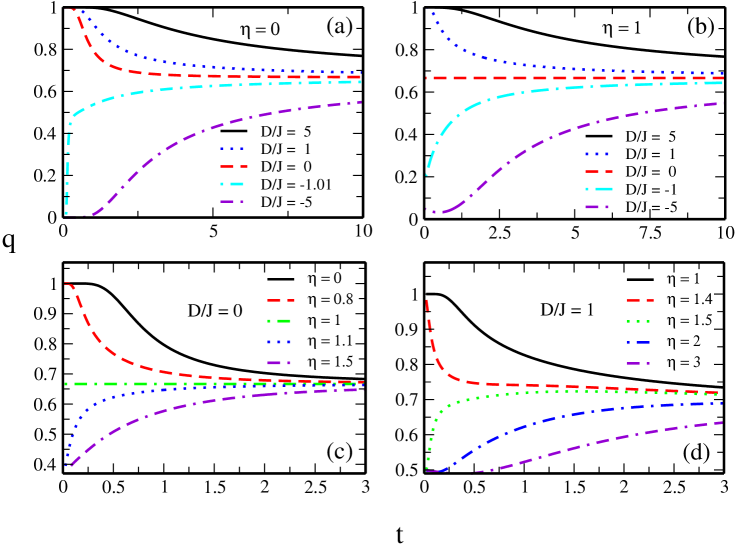
Figure 1: (color online) Quadrupole moment of the one-dimensional model, $c=2$, for several values of the Hamiltonian parameters.

III.2 Three-dimensional model

In this subsection, we present the numerical results of the behavior of the magnetization $m=\langle{S_{i}^{z}}\rangle$, the pair correlation function on the $xy$ plane $\langle{S}_{i}^{x}S_{j}^{x}+S_{j}^{x}S_{j}^{y}\rangle$ and the global phase diagrams as function of the parameters of the Hamiltonian for the three-dimensional model. The results for the two-dimensional model are qualitatively the same.

III.2.1 Magnetization and pair correlation function

In Figure 2 we show the parallel and perpendicular magnetizations as a function of the reduced temperature $t=k_{B}T/J$, for several values of $\eta$, for the three-dimensional model and $D/J=0$. In $(a)$, we have $\eta<1$ and the stable phase is the one with an Ising like ordering along the $z$ direction and exhibiting a continuous phase transition as the temperature is increased. One also notes that as the anisotropy is decreased, the quantum fluctuations increase and the critical temperature is lowered. The spin components tend to lie more in the $xy$ plane as $\eta\rightarrow 1$. On the other hand, in (b), where $\eta>1$, the stable phase is the one with a perpendicular ordering. Now, by increasing $\eta$, the easy plane tendency of the ordering is enhanced and, as a consequence, the critical temperature is also increased. However, one can see a reentrant behavior where a second continuous transition takes place at low temperatures. This reentrancy will become clearer when discussing the phase diagrams. Figure 3 depicts the magnetizations for $\eta=1$ and various values of the crystal field. In this case, two continuous transitions are seen for negative values of $D$. These reentrancies are not found in the usual mean-field approach.

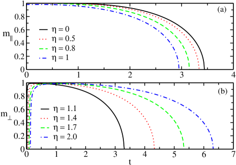
Figure 2: (color online) (a) Parallel $m_{\parallel}$ and (b) perpendicular $m_{\bot}$ magnetizations as a function of the reduced temperature $t={k_{B}T}/{J}$, for $D/J=0$, $c=6$ and several values of the anisotropy $\eta$.

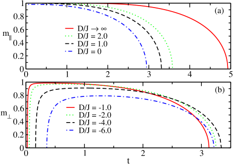
Figure 3: (color online) (a) Parallel $m_{\parallel}$ and (b) perpendicular $m_{\bot}$ magnetizations as a function of the reduced temperature $t={k_{B}T}/{J}$, for $\eta=1$, $c=6$ and several values of the crystal field $D/J$.

The nearest-neighbor pair correlation function in the $xy$ plane is shown in Figure 4 for $D/J=0$ and various values of $\eta$. For $\eta>1$, the easy plane situation, this correlation function decreases as the temperature increases, because the system is already ordered in the plane. On the other hand, for $\eta<1$, the easy axis case, the in-plane correlation function increases as the temperature increases, since the temperature tends to destroy the order along the $z$ direction, favoring in this case the $xy$ plane. The inset in Figure 4(a) shows the special case $\eta=1$, where we have a coexistence of both ordered phases, along the $z$ direction and in the $xy$ plane. The pair correlation functions behave differently in each phase, becoming equal at the tetracritical temperature (see discussion below).

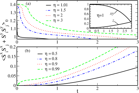
Figure 4: (color online) In-plane nearest-neighbor pair correlation function as a function of the reduced temperature for the three-dimensional model and $D/J=0$ for several values of $\eta$. (a) $\eta>1$ and (b) $\eta<1$. The inset in (a) shows the results for $\eta=1$ for the ordered phase in the $z$ direction and $xy$ plane, respectively.

III.2.2 Global Phase Diagrams

Figure 5 displays the global phase diagram in the reduced critical temperature versus reduced crystal field plane, in the three-dimensional limit, for several values of the anisotropy $\eta$. One can see that as soon as $\eta<0.33$ the phase diagram is quite similar to that of the classical Blume-Capel model, presenting second- and first-order transition lines separated by a tricritical point. In the limit $D/J\rightarrow\infty$ all curves go to the same result $t_{c}=4.932$, as discussed in the text. Apart from the reentrancy at low temperatures, which is clearly depicted in the inset, for this range of anisotropy the quantum effects seem not to be enough to change the character of the transition, and the perpendicular ordered phase is never stable. The anisotropy can only stabilize the perpendicular phase when $\eta>0.33$. This is in contrast to the simple mean-field approach, where the perpendicular order is always stable as soon as $\eta>0$khaje .

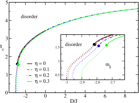
Figure 5: (color online) Global phase diagram in the reduced temperature versus crystal field for several values of the anisotropy $\eta\leq 0.3$, in the three-dimensional lattice with $c=6$. The dotted lines refer to first-order transitions and the others lines (continuous, dashed and dotted-dashed) refer to second-order phase transitions . The circles represent the tricritical points. The transition is always from the stable parallel ordered phase with $m_{\parallel}\neq 0$ to the disordered phase. The inset shows the low temperature region on a finer scale.

For $0.33<\eta<0.49$ the phase diagram looks like the one shown in Figure 6. In addition to the tricritical point one has two critical endpoints in the first-order transition line separating the parallel and perpendicular ordered phases.

Figure 6: Global phase diagram in the reduced temperature versus crystal field plane for $\eta=0.4$, in the three-dimensional lattice with $c=6$. The continuous lines refer to second-order phase transitions and the dotted line refers to first-order transition. The circle represents the tricritical point and the squares represent the critical endpoints. $m_{\parallel}$ is the parallel ordered phase and $m_{\bot}$ is the perpendicular ordered phase.

As $\eta$ increases, the tricritical and the high temperature critical endpoint approaches one another and eventually, for $\eta>0.49$, they coalesce in a tetracritical point. The phase diagram in this range of anisotropy is depicted in Figure 7.

Figure 7: Global phase diagram in the reduced temperature versus crystal field plane for $\eta=0.8$, in the three-dimensional lattice with $c=6$. The continuous lines refer to second-order phase transitions and the dotted line refers to first-order transition. The squares represent the low temperature critical endpoint and the diamond represents the tetracritical point. $m_{\parallel}$ is the parallel ordered phase and $m_{\bot}$ is the perpendicular ordered phase. The inset shows a closer view of the low temperature region.

For $\eta=1$ the first-order transition line separating the perpendicular and the parallel phases is a straight vertical line at $D/J=0$, as shown in Figure 8 together with a comparison to the usual mean-field approximation (or one-spin approach)khaje . Comparing to the mean-field results one can see that the critical temperature from the pair approximation is systematically below those by taking just one-spin cluster. The reentrancy only occurs for the pair approximation. Similar results are obtained for other values of $\eta>1$, with the slope of the first-order transition line between the ordered phases becoming positive in this range.

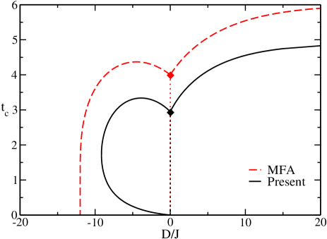
Figure 8: (color online) Phase diagram in the reduced temperature versus crystal field plane for $\eta=1$, in the three-dimensional lattice with $c=6$, according to the present approach in comparison to the MFA. The continuous and dashed lines refer to second-order phase transitions and the dotted lines refer to first-order transition. The diamonds represent the the tetracritical point.

Figure 9: Reduced crystal field $D/J$ as a function of the anisotropy $\eta$, at zero temperature $T=0$, for the three-dimensional model.

All of the above results refer to the three-dimensional model with coordination number $c=6$. The same holds for the two-dimensional model. It means that in this case, for spin $S=1$, one does not get the Mermin and Wagner result $T_{c}=0$ for $\eta=1$ and $D=0$. However, we believe the approach is suitable to the three-dimensional system, mainly when we compare the critical temperatures, as depicted in Table 1.

III.3 Quantum Phase Diagram $T=0$

From Figures 5-8, we note that for each anisotropy there exists a value for the crystal field $D/J$ in which there is a transition at $t=0$. This transition happens to be of first order and it is illustrated in Figure 9. One cannot find neither a second-order quantum phase transition nor a quantum tricritical point according to the present pair procedure, in contrast to the simple mean-field approach where there is always a quantum phase transition at zero temperature. It should be stressed, however, that there is a rigorous proof of the existence of only first-order phase transitions at low temperature and large anisotropy for the XXZ model bob .

IV concluding remarks

The anisotropic spin-$1$ XXZ quantum Heisenberg model in a crystal field has been studied according to a variational approach for the free energy by using a pair approximation. This procedure enables one to get the ordering along the $z$ direction and in the $xy$ plane as well. Earlier pair like approaches on the same system could only take into account the parallel ordering.

As expected, the one-dimensional model has no phase transition and the quadrupole moment so obtained are expected to be close to exact one for $\eta>0$. So, contrary to the simple mean-field approximation, the present pair approach can distinguish the dimensionality of the lattice and much more novel information is obtained regarding the free-energy and quadrupole moment for $c=2$.

From the free energies one gets the complete phase diagrams for dimensions greater than one, which are indeed much richer than those from the simple mean-field procedure. The diagrams exhibit second- and first-order transition lines, tricritical and tetracritical points, as well as critical end points. Although for the spin-$1$ case we do not reproduce the Mermin-Wagner theorem in the two-dimensional case, we believe the results are appropriate for the three-dimensional model. Of course, as it is still a mean-field approach, it should be necessary more reliable methods to corroborate the reentrancies observed in some range of the Hamiltonian parameters.

Appendix A

In this appendix we present the expressions for the coefficients $a_{2}^{\parallel}(t,D,\eta)$, $a_{4}^{\parallel}(t,D,\eta)$ and $a_{2}^{\bot}(t,D,\eta)$ appearing in the Landau expansion for the free energy (37) at the subsection II.3. Before writing these coefficients, we will define the following variables

$$\epsilon = \frac{{\cal Z}_{2\parallel}^{p}(0)}{2e^{\beta(D+\gamma_{2}^{\parallel})}(\cosh(\beta{J}\eta)+2e^{\beta(J+D+\gamma_{2}^{\parallel})})},$$

$$A = \frac{2e^{\beta(D+\gamma_{1}^{\parallel})}}{{\cal Z}_{1\parallel}^{f}(0)},$$

$$B = \frac{A}{6}-\frac{A^{2}}{2},$$

$$I = e^{\beta(D+\gamma_{2}^{\parallel})}(\cosh(\beta{J}\eta)+8e^{\beta(J+D+\gamma_{2}^{\parallel})}),$$

where ${\cal Z}_{1\parallel}^{f}(0)$ and ${\cal Z}_{2\parallel}^{p}(0)$ are given by equations (25) and (26).

So, we can write

$$a_{2}^{\parallel} = \frac{(1-c)}{2A}-\frac{c\epsilon}{2},$$

$$a_{4}^{\parallel}=\frac{B(c-1)}{4A^{4}}-\frac{cI{\epsilon}^{4}}{2{\cal Z}_{2\parallel}^{p}(0)}+\frac{z{\epsilon}^{2}}{4},$$

$$a_{2}^{\bot} = \frac{2c[e^{\beta(D+\gamma_{1}^{\bot})}-1]}{(1-c)(D+\gamma_{1}^{\bot}){\cal Z}_{1\bot}^{f}(0)}-\frac{\sum_{i}e^{-\beta\delta_{i}}\Gamma_{i}}{{\cal Z}_{2\bot}^{p}(0)},$$

where ${\cal Z}_{1\bot}^{f}(0)$, ${\cal Z}_{2\bot}^{p}(0)$ and $\sum_{i}e^{-\beta\delta_{i}}\Gamma_{i}$ are given by equations (31), (32), and (33), respectively.

References

• (1) Giovannetti et al, Nature Communications 2, 398 (2011).
• (2) T. R .Kirkpatrick1 and D. Belitz, Phys. Rev. B 85, 134451 (2012).
• (3) M. Uhlarz, C. Pfleiderer and S. M. Hayden, Phys. Rev. Lett. 93, 256404 (2004).
• (4) J. Hertz, Phys. Rev. B 14, 1165 (1976).
• (5) Sondhi et al, Rev. Mod. Phys. 69, 315 (1997).
• (6) K. R. Hazzard, Quantum Phase Transitions in Cold Atoms and Low Temperature Solids Springer, Ithaca (2011).
• (7) L. D. Carr, Understanding Quantum Phase Transitions (Condensed Matter Physics), CRC Press (2010).
• (8) Bitko et al Phys. Rev. Lett. 77, 940 (1996).
• (9) B. Keimer et al Phys. Rev. B 46, 14034 (1992).
• (10) T. Mikasawa, Y. Yamaji and M. Imada, J. Phys. Soc. Jpn. 78, 084707 (2009).
• (11) S. Sachdev, Quantum Phase Transitions, Cambridge University Press, Cambridge (1999).
• (12) W. Shiramura et al, J. Phys. Soc. Jpn. 67, 1548 (1998).
• (13) P. Pfeuty, Ann. Phys. 57, 79 (1970).
• (14) J. B. Kogut, Rev. Mod. Phys. 51, (1979).
• (15) D. C. Carvalho J. A. Plascak and L. M. Castro, Physica A 391 (2012).
• (16) A. S. T. Pires, Sol. State Comm. 100, 791 (1996).
• (17) A. S. T. Pires, Journal of Magnetism and Magnetic Materials 323, 1977 (2011).
• (18) V. S. Abgaryan et al, arXiv:1106.5378v1 [cond-mat.stat-mech], (2011).
• (19) M. E. Fisher, Am. J. Phys. 32, 343 (1964).
• (20) H. Bethe, Z. Physik A 71, 205 (1931).
• (21) N.D. Mermin and H. Wagner, Phys. Rev. Lett. 17, 1133 (1966).
• (22) J.H. Van Vleck, Phys. Rev 41: 208 (1932).
• (23) J.H. Van Vleck, The Theory of Electric and Magnetic Susceptibilities, Oxford University Press, 1932.
• (24) H. Bethe, Ann. Physik 3 133 (1929).
• (25) Crystalline Electric Field and Structural Effect in f-Electron Systems, edited by J. E. Crow, R. P. Gruertin, and T. W. Mihalisin (Plenum, New York, 1980).
• (26) C. Pfleiderer and A. D. Huxley, Phys. Rev. Lett. 89, 147005 (2002).
• (27) M. Blume, Phys. Rev. 141 517 (1966).
• (28) H. W. Capel, Physica 32 966 (1966).
• (29) J.A. Plascak, J.G. Moreira and F.C. S. Barreto, Phys. Lett. A173, 360 (1993).
• (30) D. Peña Lara and J. A. Plascak, Mod. Phys. Lett. B 10 1067 (1996).
• (31) D. Peña Lara and J. A. Plascak, Int. J. Mod. Phys. 12 2045 (1998).
• (32) A. K. Jain and D. P. Landau, Phys. Rev. B 22: 445 (1980).
• (33) J. A. Plascak and D. P. Landau, Phys. Rev. E 67, R015103 (2003).
• (34) C. J. Silva, A. A. Caparica, and J. A. Plascak, Phys. Rev. E 73, 036702 (2006).
• (35) J. C. Xavier, F. C. Alcaraz, D. Peña Lara, and J. A. Plascak, Phys. Rev. B 57 11575 (1998).
• (36) V.A. Schmidt and S.A. Friedberg, Phys. Rev. 1 2250 (1970).
• (37) J. Oitmaa and C.J. Hamer, Phys. Rev. B 77, 224435 (2008).
• (38) M. Blume, V. J. Emery, and R. B. Griffths, Phys. Rev. A 4, 1071 (1971).
• (39) G. P. Taggart, R. A. Tahir-Kheli and E. Shiles, Physica 75, 234 (1974).
• (40) M. R. H. Khajehpour, Yung-Li Wang and Robert A. Kromhout, Phys. Rev. 12, 1849 (1975).
• (41) Kok-Kwei Pan and Yung-Li Wang, Phys. Rev. B 51, 3610 (1995).
• (42) J. Strecka, J. Dely and L. Canova, Chinese J. Phys 46, 329 (2008).
• (43) H. Falk, Am. J. Phys. 38, 858 (1970).
• (44) L. G. Ferreira, S. R. Salinas and M. J. Oliveira, Phys. Status Sol.(b) 83, 229 (1977).
• (45) L. Onsager, Phys. Rev. 65 117 (1944).
• (46) A. M. Ferrenberg and D. P. Landau, Phys. Rev. B 44, 5081 (1991).
• (47) I.G. Enting, A.J. Guttmann and I. Jensen, J. Phys. A: Math. Gen. 27, 6987 (1994).
• (48) P. Butera and M. Comi, Phys. Rev. B 65, 144431 (2002).
• (49) H. E. Stanley and T. A. Kaplan, Phys. Rev. Lett. 17 913 (1966).
• (50) C. C. Song, Y. Cheng and M.-W Liu, Physica B 405 439 (2010).
• (51) T. Balcerzak and I.Łużniak, Physica A 388, 357 (2009).
• (52) R. W. Robinson, Commun. math. Phys. 14, 195 (1969).