Power of the redshift drift on cosmological models and expansion history

Abstract

We investigate the power of the velocity drift ($\Delta v$) on cosmological parameters and expansion history with observational Hubble data (OHD), type Ia supernova (SNIa). We estimate the constraints of $\Delta v$ using the Fisher information matrix based on the model by Pasquini et al. (2005, 2006a). We find that $\Delta v$ with 20 years can reduce the uncertainty of $\Omega_{m}$ by more than 42% than available observations. Based on the statistical figures of merit (FoM), we find that in order to match the constraint power of OHD and SNIa, we need 21 and 26 future measurements, respectively. We also quantitatively estimate for the first time the number of years required for the velocity drift to become comparable with current observations on the equation of state $w$. The statistical FoM indicate that we need at least 12 years to cover current observations. Physically, we could monitor 30 quasars for 30 years to obtain the same accuracy of $w$. Considering two parameterized deceleration factor $q(z)$, we find that the available observations give an estimation on current value $-0.9\lesssim q_{0}\lesssim-0.3$. Difference between the two types of $q(z)$ is the precise determination of variation rate $dq/dz$. For the first model with constant $dq/dz$, $\Delta v$ with only 10 years provides a much better constraint on it, especially when compared with SNIa. However, we need $\Delta v$ for more years in the variable $dq/dz$ model. We find that $\Delta v$ with 30 years reduces the uncertainty of transition redshift to approximately three times better than those of OHD and SNIa.

1. Introduction

Cosmological observations probe an accelerating expansion of the universe. Examples include Type Ia supernova (SNIa) observations (Riess et al. 2007), Large Scale Structure (Tegmark et al. 2004), and Cosmic Microwave Background (CMB) anisotropy (Spergel et al. 2003). As a key factor that reflects the expansion history of the universe, the Hubble parameter $H=\dot{a}/a$ relevant to various observations. In practice, we measure the Hubble parameter as a function of redshift $z$. Observationally, we can deduce $H(z)$ from differential ages of galaxies (Jimenez & Loeb 2008; Simon et al. 2005; Stern et al. 2010), from the baryon acoustic oscillation (BAO) peaks in the galaxy power spectrum (Gaztanaga et al. 2009; Moresco et al. 2012) or from the BAO peak using the Ly$\alpha$ forest of quasars (Busca et al. 2013). We can theoretically reconstruct $H(z)$ from the luminosity distances of SNIa using their differential relations (Wang & Tegmark 2005; Shafieloo et al. 2006; Mignone & Bartelmann 2008). The available observational Hubble parameter data (OHD) have been applied in the standard cosmological model (Lin et al. 2009; Stern et al. 2010), and in some other FRW models (Samushia & Ratra 2008; Zhang et al. 2010b; Zhai et al. 2011). Furthermore, the potential of future $H(z)$ observations in parameter constraint has also been explored (Ma & Zhang 2011).

SNIa present another widely used observational data in cosmology research. They give a redshift-distance relationship, the difference between apparent magnitude and absolute magnitude. SNIa have 580 data points in the latest Union2.1 compilation (Suzuki et al. 2012). Nevertheless, the rich abundance of the data still can not hide their limitations in determining the equation of state (EoS) (Garnavich et al. 1998; Maor et al. 2001) and current deceleration factor $q_{0}$ (Phillipps 1983) of the universe. Meanwhile, there have been studies of the limitations in brane world cosmology (Fairbairn & Goobar 2006) and neutrino radiative lifetimes (Falk & Schramm 1978).

Actually, limitations of current observations are mainly attributed to their measurement relations and model assumptions. For example, previous CMB, SNIa, weak lensing and BAO, are essentially geometric. In 1962, Sandage (1962) proposed a promising dynamical survey named redshift drift to directly probe the dynamics of the expansion. Unlike previous observations, the redshift drift measures the secular variation of expansion rate into a deeper redshift of $z=2-5$. It can provide useful information about the cosmic expansion history in the “redshift desert”, where other probes are far behind. Unfortunately, extremely weak theoretical magnitude indicates that it is difficult to detect. For example, the redshift drift $\Delta z$ within a 10-year observational time interval for a source at this redshift coverage has a magnititude of an order of only $10^{-9}$. The corresponding velocity drift $\Delta v$ is also inappreciable as only several cm/s. Fortunately, Loeb (1998) developed a possible scheme from the wavelength shift of quasar (QSO) Ly$\alpha$ absorption lines. A new generation of COsmic Dynamics EXperiment (CODEX) with a high resolution, extremely stable and ultra high precision spectrograph is now available, capable of measuring such a small cosmic signal in the near future (Pasquini et al. 2005, 2006b). Based on the power of CODEX, some groups generate velocity drift by Monte Carlo simulation with the assumption of standard cosmological model (Liske et al. 2008a, b, 2009). These simulations investigate the constraints in holographic dark energy (Zhang et al. 2007), modified gravity models (Jain & Jhingan 2010), new agegraphic and Ricci dark energy models (Zhang et al. 2010a) are investigated. They found that the velocity drift can provide constraints on models with high significance. In addition, Balbi & Quercellini (2007) evaluate the redshift drift from several dark energy models. However, this evaluation of the power of the redshift drift among current observations is mostly qualitative, not quantitatively. In this study, we wish to investigate how many data points or years of future redshift drift or velocity drift observations could provide valid constraints on cosmological parameters as good as those from OHD or SNIa? Furthermore, could future velocity drift data offer more accurate information about the expansion history?

We attempt to answer these questions via an exploratory, statistical approach. This paper is organized as follows: In Section 2, we introduce the basic theory of the redshift drift. Then, we analyze the sensitivity of cosmological parameters to the Hubble parameter, luminosity distance and the velocity drift. Section 3 presents a statistical analysis of these observations and evaluates the constraint. Section 4 gives results of constraints in specific evaluation models. In Sec. 5, we compare constraints of these observations on two models of deceleration factor $q(z)$. Finally, Section 6 presents our main results and discussion.

2. Basic theory

2.1. Redshift drift

Since the birth of the redshift drift, many observational candidates like masers and molecular absorptions were put forward, but the most promising one appears to be the Ly$\alpha$ forest in the spectra of high-redshift QSOs (Pasquini et al. 2006b). These spectra are not only distinct from the noise of the peculiar motions relative to the Hubble flow, but also have a large number of lines in a single spectrum (Pasquini et al. 2005). In particular, Pasquini et al. (2005) have found that 25 QSOs are presently known at redshift $z=2-4$ with a magnitude brighter than 16.5. Recently, Darling (2012) shows a set of observational redshift drift from the precise HI 21 cm absorption line using primarily Green Bank Telescope digital data. These measurements last 13.5 years for ten objects spanning a redshift of $z=0.09-0.69$. Table 1 of Darling (2012) shows that main redshift drift in this redshift coverage are of order $10^{-8}$ yr^-1, which is about three orders of magnitude larger than the theoretical values. The author ascribes this discrepancy to the lack of knowledge on the peculiar acceleration in absorption line systems and to the long-term frequency stability of modern radio telescopes.

For an expanding universe, a signal emitted by the source at time $t_{\mathrm{em}}$ was observed at $t_{0}$. We represent the source’s redshift through a cosmic scale factor

$$z(t_{0})=\frac{a(t_{0})}{a(t_{\mathrm{em}})}-1.$$ (1)

Over the observer’s time interval $\Delta t_{0}$, the source’s redshift becomes

$$z(t_{0}+\Delta t_{0})=\frac{a(t_{0}+\Delta t_{0})}{a(t_{\mathrm{em}}+\Delta t_{\mathrm{em}})}-1,$$ (2)

where $\Delta t_{\mathrm{em}}$ is the time interval-scale when the source emits another signal. It should satisfy $\Delta t_{\mathrm{em}}=\Delta t_{0}/(1+z)$. We represent the observed redshift variation of the source by

$$\Delta z=\frac{a(t_{0}+\Delta t_{0})}{a(t_{\mathrm{em}}+\Delta t_{\mathrm{em}})}-\frac{a(t_{0})}{a(t_{\mathrm{em}})}.$$ (3)

A further relation can be obtained if we keep the first order approximation

$$\Delta z\approx\left[\frac{\dot{a}(t_{0})-\dot{a}(t_{\mathrm{em}})}{a(t_{\mathrm{em}})}\right]\Delta t_{0}.$$ (4)

Clearly, the observable $\Delta z$ is a direct change of the expansion rate during the evolution of the Universe. In terms of the Hubble parameter $H(z)=\dot{a}(t_{\mathrm{em}})/a(t_{\mathrm{em}})$, it can simplify as

$$\frac{\Delta z}{\Delta t_{0}}=(1+z)H_{0}-H(z).$$ (5)

This is also well known as McVittie equation (McVittie 1962). Obviously, cosmological models associate with the redshift drift just through the Hubble parameter $H(z)$. Taking a standard cosmological model as an example, we find that redshift drift at low redshift generally towards to negative with the dominance of matter density parameter $\Omega_{m}$. This feature is often used to distinguish dark energy models from LTB void models at $z<2$ (especially at low redshift) (Yoo et al. 2011). Unfortunately however, the scheduled CODEX would not be able to measure this drift at low $z$ (Liske et al. 2008a). Observationally, it is more common to detect the spectroscopic velocity drift

$$\frac{\Delta v}{\Delta t_{0}}=\frac{c}{1+z}\frac{\Delta z}{\Delta t_{0}},$$ (6)

which is in order of several cm s^-1 yr^-1. Obviously, the velocity variation $\Delta v$ can be enhanced with the increase of observational time $\Delta t_{0}$.

For the capability of CODEX, the accuracy of the spectroscopic velocity drift measurement was estimated by Pasquini et al. (2005, 2006a) from Monte Carlo simulations. It can be modelled as

$$\sigma_{\Delta v}=1.4\left(\frac{2350}{\textrm{S/N}}\right)\left(\frac{30}{N_{\textrm{QSO}}}\right)^{1/2}\left(\frac{5}{1+z_{\textrm{QSO}}}\right)^{1.8}\mathrm{cm/s},$$ (7)

where S/N is the signal-to-noise ratio, $N_{\textrm{QSO}}$ and $z_{\textrm{QSO}}$ are respectively the number and redshift of the observed QSO. According to currently known QSOs brighter than 16.5 with $2\lesssim z\lesssim 4$, Pasquini et al. (2005, 2006a) assumed to observe either 40 QSOs with S/N ratio of 2000, or 30 QSOs with S/N of 3000, respectively. In this paper, our investigations are based on the latter. Unless stated otherwise, the observational time is $\Delta t_{0}=10$ years.

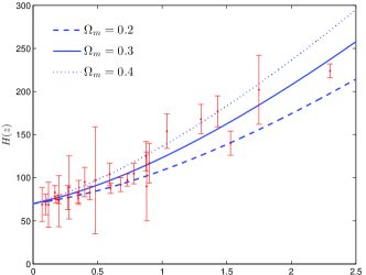
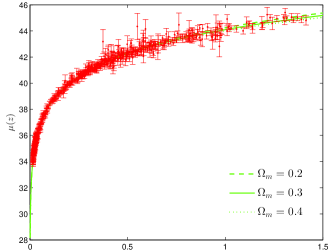
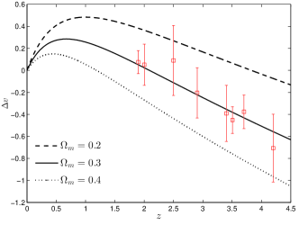
Figure 1.— Evolution of Hubble parameter, distance modulus and velocity drift for the flat $\Lambda$CDM model with different $\Omega_{m}$.

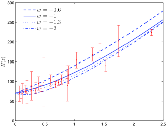
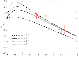
Figure 2.— Same as Figure 1 but for the flat XCDM model. Dark energy density is fixed at $\Omega_{\Lambda}=0.7$ but for different EoS $w$.

2.2. Sensitivity comparison

In fact, most cosmological models can fit well with the observations. It is difficult to distinguish or rule out some models. In this paper, we mainly compare the velocity drift with the OHD and SNIa. For further understanding on some fundamental parameters, the fiducial cosmological models here are taken as flat $\Lambda$CDM model and XCDM model.

Changing matter density $\Omega_{m}$ from 0.2 to 0.4, we plot the Hubble parameter $H(z)$, distance modulus $\mu(z)$ and velocity drift $\Delta v$ for the $\Lambda$CDM model in Figure 1. Intuitively, we find that the theoretical curves respectively deviate from each other with different degree. In which, difference of $\Delta v$ for different $\Omega_{m}$ becomes remarkable with the increase of redshift. In order to eliminate the effect of different units, we take into account the observational data. OHD are the latest available sample covering redshift $0.07\leqslant z\leqslant 2.3$ (Farooq & Ratra 2013). The updated Union2.1 compilation of SNIa is compiled by Suzuki et al. (2012). Eight points of $\Delta v$ are simulated by Liske et al. (2008a, b, 2009) for 20 years. We find that most of current OHD at $z<1$ can not distinguish these models, and can not steadily favor a specific model at $z>1$. While $\mu(z)$ seem to be attracted on the theoretical curves with little discrimination. Fortunately, only $\Delta v$ strongly supports the model with $\Omega_{m}\sim 0.3$. Different sensitivities show that $\Delta v$ is a possible effective tool to discriminate $\Lambda$CDM model or accurately determine the matter density, which agree with the previous investigation (Zhang et al. 2007; Jain & Jhingan 2010).

In Figure 2, we plot these three parameters for the flat XCDM model with fixed $\Omega_{\Lambda}=0.7$. In order to emphasize the influence of equation of state (EoS) on these parameters, we change EoS $w$ from -0.6 to -2. Same as above model, $\mu(z)$ in this case is still insensitive to parameter $w$. Unlike above case, however, $H(z)$ and $\Delta v$ both are not sensitive to $w$ as long as $w<-0.6$. However, as estimated from Equation (6), signals can be linearly enhanced with the increase of observational interval time $\Delta t_{0}$. Therefore, we possibly investigate $\Delta v$ for several different years in following analysis. Moreover, different magnitudes of $\Delta v$ at $z\approx 0.5$ indicate that velocity drift at low redshift may be an effective scheme to distinguish different dark energy candidates.

3. Observational constraints

In order to explore the answer to questions raised in Section 1, we respectively introduce constraint methods. OHD and SNIa are available to determine parameters by the $\chi^{2}$ statistics. When observation is absent or not enough, we can forecast constraint by the Fisher matrix. Constraint from velocity drift is just finished using this approach.

3.1. Hubble parameter

As introduced above, OHD can be measured through the differential age of passively evolving galaxies and the BAO peaks. We use the latest available data listed in Table 1 of Farooq & Ratra (2013). Parameters can be estimated by minimizing

$$\chi^{2}_{\textrm{OHD}}(H_{0},z,\textbf{p})=\sum_{i}\frac{[H_{0}E(z_{i})-H^{obs}(z_{i})]^{2}}{\sigma_{i}^{2}},$$ (8)

where p stands for the parameters vector of each dark energy model embedded in expansion rate parameter $E(z_{i})$. In order to terminate disturbance of the “nuisance” parameter, Hubble constant $H_{0}$ is integrated as a prior according to the Planck Collaboration et al. (2013) suggestion, $H_{0}=67.3\pm 1.2$ km s^-1Mpc^-1.

3.2. Luminosity distance

SNIa is famous for its rich abundance of data. The latest Union2.1 compilation (Suzuki et al. 2012) accommodates 580 samples. The future SuperNova Acceleration Probe (SNAP) mission is said to be able to gather high-signal-to-noise calibrated light-curves and spectra for over 2000 SNIa per year at $0<z<1.7$ (Aldering et al. 2002). They are usually presented in the shape of distance modulus, the difference between the apparent magnitude $m$ and the absolute magnitude $M$

$$\mu_{\textrm{th}}(z)=m-M=5\textrm{log}_{10}D_{L}(z)+\mu_{0},$$ (9)

where $\mu_{0}=42.38-5\textrm{log}_{10}h$, and $h$ is the Hubble constant $H_{0}$ in units of 100 km s^-1Mpc^-1. The corresponding luminosity distance function $D_{L}(z)$ can be expressed as

$$D_{L}(z)=\frac{1+z}{\sqrt{\left|\Omega_{k}\right|}}\operatorname{sinn}\left[\sqrt{\left|\Omega_{k}\right|}\int^{z}_{0}\frac{\mathrm{d}z^{\prime}}{E(z^{\prime};\textbf{p})}\right],$$ (10)

where the $\operatorname{sinn}$ function therein is a shorthand for the definition

$$\operatorname{sinn}(x)=\begin{cases}\sinh x,&\Omega_{k}>0,\\ x,&\Omega_{k}=0,\\ \sin x,&\Omega_{k}<0.\end{cases}$$ (11)

Parameters in the expansion rate $E(z^{\prime};\textbf{p})$ including the annoying parameter $h$ commonly determined by the Equation (8) but replacing Hubble parameter as distance modulus. However, an alternative way can marginalize over the “nuisance” parameter $\mu_{0}$ (Pietro & Claeskens 2003; Nesseris & Perivolaropoulos 2005; Perivolaropoulos 2005). The rest parameters without $h$ can be estimated by minimizing

$$\chi^{2}_{\textrm{SN}}(z,\textbf{p})=A-\frac{B^{2}}{C},$$ (12)

where

$$A(\textbf{p}) = \sum_{i}\frac{[\mu_{\textrm{obs}}(z)-\mu_{\textrm{th}}(z;\mu_{0}=0,\textbf{p})]^{2}}{\sigma_{i}^{2}(z)},$$

$$B(\textbf{p}) = \sum_{i}\frac{\mu_{\textrm{obs}}(z)-\mu_{\textrm{th}}(z;\mu_{0}=0,\textbf{p})}{\sigma_{i}^{2}(z)},$$

$$C = \sum_{i}\frac{1}{\sigma_{i}^{2}(z)}.$$ (13)

It is equivalent with the general form like Equation (8). However, difference from the $\chi^{2}_{\textrm{OHD}}$ statistics is that $H_{0}$ in this operation is marginalized over by Gaussian integration over ($-\infty,\infty$) without any prior. This program has been used in the reconstruction of dark energy (Wei et al. 2007), parameter constraint (Wei 2010), reconstruction of the energy condition history (Wu et al. 2012) etc.

3.3. Velocity drift

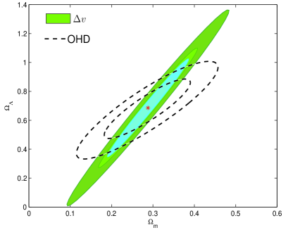
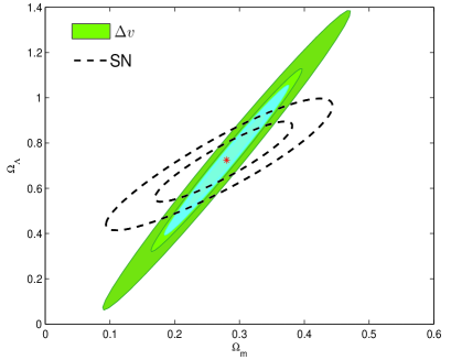
Figure 3.— Constraints on the parameters ($\Omega_{m}$, $\Omega_{\Lambda}$) for the $\Lambda$CDM model. The contours show the 68% and 95% C.L., respectively. Dashed curves are contours from available observations. Green shaded regions and blue shaded regions are contour constraints of $\Delta v$ for 10 years and 20 years observational time, respectively.

Fisher information matrix (Jungman et al. 1996; Vogeley & Szalay 1996; Tegmark et al. 1997; Tegmark 1997) could help velocity drift to provide estimation on parameters. This forecast is a second-order approximation to the likelihood, and has become an important strategy on parameter constraints in recent years. Its normal form for velocity drift is

$$F_{ij}=\sum\frac{1}{\sigma_{\Delta v}^{2}}\frac{\partial\Delta v}{\partial\theta_{i}}\frac{\partial\Delta v}{\partial\theta_{j}},$$ (14)

where $\sigma_{\Delta v}$ are errors of $\Delta v$ which has been estimated from Equation (7), $\theta_{i}$ denotes the $i$th parameter. For comparison, parameters of Equation (14) in the fiducial model are respectively taken to be the best-fit ones from OHD and SNIa. Therefore, the Fisher matrix elements, in practice, can be estimated. Eventually, we can compare the constraint power of $\Delta v$ with OHD and SNIa, respectively. With the Fisher matrix, we can estimate the uncertainty of parameter $\theta_{i}$ through its inverse

$$\Delta\theta_{i}\geqslant\sqrt{(F^{-1})_{ii}}.$$ (15)

The sign $\geqslant$ results from the Cramer-Rao theorem which states that any unbiased estimator for the parameters is no better than that from $F^{-1}$. However, on many occasions we need to produce a Fisher matrix in a smaller parameter space. Similar to above approach on OHD and SNIa, it can be finished by adding a prior or marginalizing over the undesired “nuisance” parameter. We use the standard technique issued by the Dark Energy Task Force (DETF) in XIII. Technical Appendix (Albrecht et al. 2006).

Prior.— Based on the DETF, we can adopt a Gaussian prior with error $\sigma$ to the corresponding parameter by adding a new Fisher matrix $\textbf{F}^{P}$ with a single non-zero diagonal element $1/\sigma^{2}$

$$\textbf{F}\rightarrow\textbf{F}+\textbf{F}^{P}.$$ (16)

For example, $H_{0}$ should be disposed as a prior when we compare $\Delta v$ with OHD. In this case, we can simply add $1/\sigma_{H}^{2}$ to $F_{jj}$ where $H_{0}$ locates.

Marginalization.— When our attention does not focus on some nuisance parameters without any additional prior, we can directly marginalize over them. In the $\chi^{2}$ statistics, marginalization is usually defined by integrating the probabilities on specific nuisance parameter $\theta_{i}$

$$\bar{\chi}^{2}=-2\textrm{ln}\left(\int^{+\infty}_{-\infty}e^{-\chi^{2}/2}d\theta_{i}\right).$$ (17)

The Equation (12) is just accomplished by this method to marginalize over parameter $H_{0}$ in normal $\chi^{2}$ statistics. However, in DETF there is a simple way to do this for the Fisher matrix: Invert F, remove the rows and columns that are being marginalized over, and then invert the result to obtain the reduced Fisher matrix (Albrecht et al. 2006).

3.4. Figure of merit

Figure of merit (FoM) is an useful approach to quantitatively evaluate the constraining power of cosmological data. It has been used to evaluate constraint power of some simulated data on the dark energy EoS (Albrecht et al. 2006, 2009; Acquaviva & Gawiser 2010; Wang et al. 2010; Ma & Zhang 2011), or to choose which available data combination is optimal (Wang 2008; Mortonson et al. 2010). Nevertheless, we note that some versions of FoM are proposed, such as the DETF to constrain ($w_{0}$, $w_{a}$) (Albrecht et al. 2006), a simple one from constraint area (Mortonson et al. 2010) or a generalized one from determinant of the covariance matrix (Wang 2008). Recently, Sendra & Lazkoz (2012) investigate their relations. Moreover, Linder (2006) tests the concept with significant accuracy. In fact, these concepts in essence are unanimous, namely reward a tighter constraint but punishing a looser one. In this paper, we use a statistical definition (Mortonson et al. 2010) similar to above ones

$$\textrm{FoM}\approx\frac{6.17\pi}{A_{95}},$$ (18)

where $A_{95}$ is the enclosed area of constrained parameters space at 95% confidence. For this version, we will marginalize over some undesired parameters as insurance for 2D constraint. Obviously, the smaller the area is, the larger the FoM becomes. One remark is that our definition of FoM is purely statistical rather than physical.

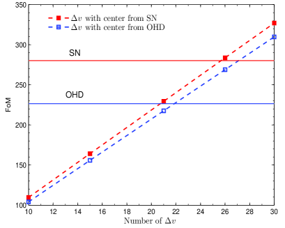
Figure 4.— FoM of each observation for the $\Lambda$CDM model. Horizontal lines across the figure mark the FoM of OHD and SNIa. Dashed lines are FoMs of $\Delta v$ from the Fisher matrix forecast with 10 years. Line marked with face is estimated at central values constrained by SNIa, while line without face is from that of OHD.

4. Results for the evaluation models

In order to comprehend cosmological density parameters and EoS, we respectively evaluate above observational data for a standard non-flat $\Lambda$CDM model and XCDM model.

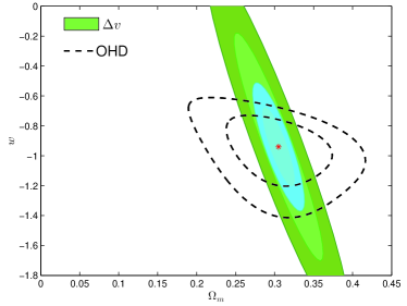
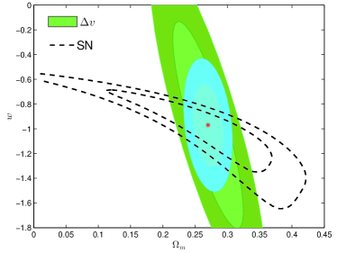
Figure 5.— Joint two-dimensional marginalized constraint on parameters ($\Omega_{m}$, $w$) of the XCDM model. Dashed lines are contours from observational data. Green shaded regions and blue shaded regions are contour constraints of $\Delta v$ for 10 years and 30 years observational time, respectively.

4.1. $\Lambda$CDM model

In the $\Lambda$CDM model, cosmological constant is believed to be the impetus of the accelerating expansion. The Hubble parameter in such model is given by

$$H(z)=H_{0}\sqrt{\Omega_{m}(1+z)^{3}+\Omega_{k}(1+z)^{2}+\Omega_{\Lambda}}.$$ (19)

Using the normalization condition on space curvature $\Omega_{k}=1-\Omega_{m}-\Omega_{\Lambda}$, the free parameters are ($\Omega_{m}$, $\Omega_{\Lambda}$, $H_{0}$). According to introduction in Section 3, OHD give constraints $\Omega_{m}=0.2880^{+0.0670}_{-0.0703}$ and $\Omega_{\Lambda}=0.6860^{+0.1330}_{-0.1385}$. Using the Fisher matrix of $\Delta v$ in this case, we present its constraint in Figure 3 for different years. We find that 30 QSOs with 10 years present uncertainties $\Delta\Omega_{m}=0.0790$ and $\Delta\Omega_{\Lambda}=0.2738$, a similar estimation as OHD on matter density but a larger one on dark energy. For more years, such as 20 years, uncertainties can be condensed as 0.0398 and 0.1374, respectively. Obviously, uncertainty of matter density is much tighter than that of OHD. This is predictable because of high sensitivity of $\Omega_{m}$ on velocity drift. By the $\chi^{2}$ statistics, SNIa presents a similar matter density $\Omega_{m}=0.2800^{+0.0677}_{-0.0724}$ and a little bigger dark energy density $\Omega_{\Lambda}=0.7245^{+0.1131}_{-0.1214}$. It can be seen that, power of 28 OHD on standard cosmological model is enough to match that of 580 SNIa. For the $\Delta v$ at this fiducial model, bottom panel shows that observation within 10 years is not enough to determine a better uncertainty estimations on these parameters than those of SNIa. However, we find that uncertainty estimation on $\Omega_{m}$ from $\Delta v$ within 20 years enhance much more, even its uncertainty at 2$\sigma$ confidence level can be comparable with that from SNIa at 1$\sigma$ confidence level. Specifically, our calculation indicates that uncertainty of matter density would been narrowed for 42%, i.e., $\Delta\Omega_{m}=0.0387$. In a short, ten years of $\Delta v$ are enough to determine a similar estimation as current observations on the matter density, but twenty years are needed to determine the dark energy density.

Besides the uncertainty estimation, purely statistic FoM also could provide an evaluation on observations. Inverse of the area of 95% confidence region in parameters ($\Omega_{m}$,$\Omega_{\Lambda}$) panel multiplying by a positive constant shows that FoMs of OHD and SNIa are 226.54 and 280.22, respectively. According to the constraints from OHD and SNIa, FoM of $\Delta v$ can be respectively estimated. Therefore, it is naturally divided into two groups. Modelled capability of CODEX indicates that it can accommodate 30 QSOs with S/N of 3000. We investigate different amounts of data points with 10 years. Our main results are shown in Figure 4. One may intuitively observe that the FoM of $\Delta v$ linearly increases with the size of the data set. And each FoM does not change much for different fiducial models, namely, different central values. We find that 21 $\Delta v$ lead to an FoM of 229.48, which could reach the parameter constraint power of OHD. Comparing with the SNIa, FoM of 26 $\Delta v$ data is 283.72, which could serve a similar constraint as SNIa. For 30 QSOs, FoM of $\Delta v$ has reached 327, much better than those from the observational data.

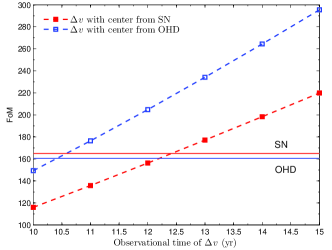
Figure 6.— FoM of each observation for the XCDM model. Marks in this figure are same as Figure 4. However, FoMs of $\Delta v$ in this case are estimated for different years with 30 QSOs.

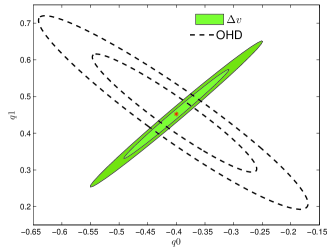
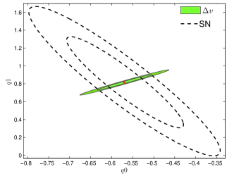
Figure 7.— Constraint on parameters ($q_{0}$, $q_{1}$) in deceleration factor of model I: $q(z)=q_{0}+q_{1}z$.

4.2. XCDM model

Expansion rate in a non-flat FRW universe with a constant EoS is given by

$$H(z)=H_{0}\sqrt{\Omega_{m}(1+z)^{3}+\Omega_{k}(1+z)^{2}+\Omega_{\Lambda}(1+z)^{3(1+w)}}.$$ (20)

Difference from the $\Lambda$CDM model is that EoS may be a value deviation from -1. Besides the cosmological constant with $w=-1$, dark energy candidates generally can be classified as quiessence with $-1<w<0$, quintessence with $-1<w<1$, and phantom with $w<-1$.

Figure 2 shows that these observations are difficult to distinguish dark energy candidates. It can be witnessed in this section. Same operation as above model, OHD give $w=-0.94^{+0.1373}_{-0.1596}$ slightly off cosmological constant. After marginalizing over the residual dark energy density parameter, matter density parameter and $w$ present a closed contour relation as shown in top panel of Figure 5. Nevertheless, constraint of $\Delta v$ in this case for 10 years is not optimistic. It is mainly because of looser uncertainty estimation on $w$. With increase of observational time, we find that power of $\Delta v$ on $w$ with 30 years could be comparable with OHD. From ten to thirty years, uncertainties of $w$ from $\Delta v$ correspondingly improve from 0.5028 to 0.1729, which reduces the $\Delta w$ by a factor of three. Meanwhile, $\Delta\Omega_{m}$ in this case for velocity drift is 0.0133, which is superior than OHD three times.

For the SNIa, they present an estimation near the cosmological constant, $w=-0.97^{+0.1985}_{-0.2250}$. $\Delta v$ in this model for 10 years does not place a tight constraint on $w$, but a better constraint on $\Omega_{m}$. Increasing the observational time for 10 years to 30 years, $\Delta w$ could improve from 0.5536 to 0.2176. That is, physically, at least thirty years are needed to catch the constraint power of current observations. Moreover, $\Omega_{m}$ in this case is almost constrained with no degeneracy. The $\Delta v$ constraint with 30 years is almost orthogonal to that provided by SNIa, which also provide a possibility that joint constraints between them may determine parameters with high significance.

Making the measurement of FoM, OHD and SNIa provide an FoM of 160.5 and 164.9, respectively. Unlike above model, they are largely identical but with minor differences. Assuming 30 QSOs are monitored, we could extend the observational time to place tight constraint. Figure 6 shows that at least 12 years are needed to reach the FoM level of OHD and SNIa.

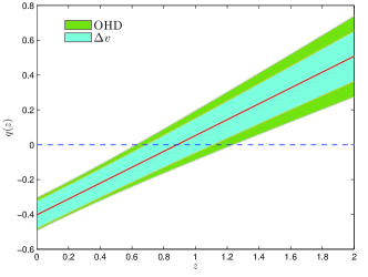
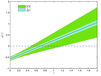
Figure 8.— Reconstruction of deceleration factor for model I: $q(z)=q_{0}+q_{1}z$, using OHD, SNIa and $\Delta v$ with 10 years.

5. Constraint on deceleration factor

As Equation (4) shown, one difference of the velocity drift aims at variation of the first derivative of cosmological scale factor. How well does this dynamical probe offer more accurate information about the expansion history? Here, we would like to investigate two parameterized deceleration factor.

Deceleration factor can be defined as

$$q(z)=-\frac{\ddot{a}}{aH^{2}}=\frac{1}{E(z)}\frac{dE(z)}{dz}(1+z)-1.$$ (21)

As known from this equation, $q(z)<0$ corresponds to the accelerating expansion, $q(z)>0$ means a deceleration. The transition redshift where the expansion of the universe switched from deceleration to acceleration is our common focus. Moreover, previous deceleration leads to $dq/dz>0$. According to the Equation (21), the dimensionless Hubble parameter can be written as

$$E(z)=\textrm{exp}\left[\int^{z}_{0}[1+q(z^{\prime})]d\textrm{ln}(1+z^{\prime})\right].$$ (22)

Finally, specific deceleration factor $q(z)$ can be reconstructed through $E(z)$ in observational variables, such as distance modulus of Equation (9) and velocity drift of Equation (6). In particular, this reconstruction no longer depends on cosmological dark energy models. Note that reconstruction from SNIa is explicitly dependent on one arbitrary constant, namely, the curvature parameter. Technically, $\Omega_{k}$ appearing in Equation (10) is marginalized. Since Riess et al. (2004) raised a linear $q(z)$, much more parameterizations have been put forward. Two ordinary models are examined here. Although they have been investigated by Cunha & Lima (2008); Cunha (2009) using different samples of Supernova Legacy Survey, our further test mainly emphasizes the power of a new future observation, i.e., the velocity drift.

5.1. model I

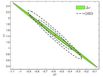
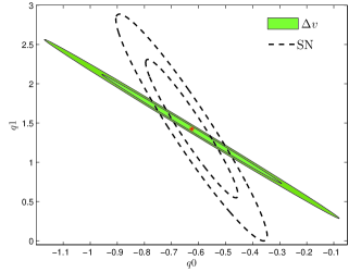
Figure 9.— Constraint on parameters ($q_{0}$, $q_{1}$) in deceleration factor of model II: $q(z)=q_{0}+q_{1}z/(1+z)$.

The simplest model for the deceleration parameter is parameterized by Riess et al. (2004)

$$q(z)=q_{0}+q_{1}z,$$ (23)

where $q_{0}$ is the deceleration factor today, constant $q_{1}$ is its change rate. Transition from deceleration to acceleration, therefore, occurs at redshift $z_{t}=-q_{0}/q_{1}$.

After a prior over $H_{0}$, OHD provide $q_{0}=-0.4^{+0.0930}_{-0.0963}$ and $q_{1}=0.4525^{+0.1064}_{-0.1057}$, which indicates a recent acceleration and previous deceleration. Uncertainties estimated by $\Delta v$ are $\Delta q_{0}=0.0802$ and $\Delta q_{1}=0.0607$, which are smaller than those of OHD, especially the variation rate. In Figure 7, individual constraints are shown. The $\Delta v$ constraint is almost orthogonal to that of the OHD. Therefore, joint constraints may help us more to break the degeneracy between $q_{0}$ and $q_{1}$. Estimations on the parameters thus can be greatly improved. The deceleration factor in Equation (23) is reconstructed by OHD in Figure 8, and a transition is found at redshift $z_{t}=0.88^{+0.3555}_{-0.2588}$, which is in good agreement with recent determination of $z_{\textrm{da}}=0.82\pm 0.08$ based on 11 $H(z)$ measurements between redshifts $0.2\leqslant z\leqslant 2.3$ (Busca et al. 2013). $\Delta v$ with 10 years gives $z_{t}=0.88^{+0.2307}_{-0.1988}$, a little tighter than OHD. We believe that much better estimation can be obtained for more years.

After marginalization over curvature $\Omega_{k}$, SNIa provide $q_{0}=-0.57^{+0.0927}_{-0.0906}$ and $q_{1}=0.815^{+0.3368}_{-0.3359}$. We find that uncertainty of $q_{0}$ between OHD and SNIa are nearly the same. But the latter presents a higher change rate $q_{1}$ and looser uncertainties. This is due to the luminosity distance, an integral relation of Hubble parameter (Sahni & Starobinsky 2000; Starobinsky 1998)

$$H(z)=\left[\frac{d}{dz}\left(\frac{D_{L}(z)}{1+z}\right)\right]^{-1}.$$ (24)

It could smear out many information about the expansion history. Reconstructed $q(z)$ in bottom panel of Figure 8 indicates a later transition at $z_{t}=0.69^{+0.5018}_{-0.2284}$, which agree with Cunha & Lima (2008); Cunha (2009). $\Delta v$ in this case estimates uncertainties $\Delta q_{0}=0.0571$ and $\Delta q_{1}=0.0427$, which are much tighter than those of SNIa. Slender outline of reconstruction realizes that the $\Delta v$ is more powerful than SNIa. A much narrower constraint is therefore obtained, $z_{t}=0.69^{+0.0813}_{-0.0774}$.

5.2. model II

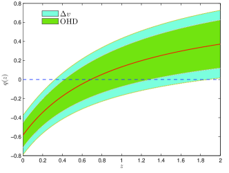
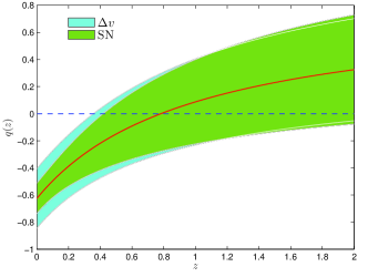
Figure 10.— Reconstruction of deceleration factor for model II: $q(z)=q_{0}+q_{1}z/(1+z)$, using OHD, SNIa and $\Delta v$ with 10 years.

Another parametrization of considerable interest is (Xu et al. 2007)

$$q(z)=q_{0}+q_{1}\frac{z}{1+z}.$$ (25)

Difference from the above is that variation rate in this model is not a constant but $dq/dz=q_{1}/(1+z)^{2}$. Transition of this model occurs at redshift $z_{t}=-q_{0}/(q_{0}+q_{1})$. Physically, in the distant past ($z\gg 0$), it leads to a constant $q(z)=q_{0}+q_{1}$.

Performing operation introduced above, parameters fitted by OHD are respectively $q_{0}=-0.5850^{+0.1308}_{-0.1318}$, $q_{1}=1.4350^{+0.3266}_{-0.3230}$. A transition is therefore estimated at $z_{t}=0.68^{+0.6054}_{-0.2718}$, later than that of model I. It is evident that the dynamical model postpone the accelerating expansion of universe. From Figure 9, pin-like constraint shape from $\Delta v$ leads to bigger uncertainties of $q_{0}$ and $q_{1}$. Naturally, reconstructed $q(z)$ from $\Delta v$ is worse than that of OHD. Evidence for this can be seen in top panel of Figure 10. Although reconstruction from $\Delta v$ with 10 years is worse, we have witnessed that its ability improves very fast with the increase of observational time. The uncertainties of transition redshift for 10 years, 20 years and 30 years are estimated to be (+1.1822, -0.3629), (+0.3693, -0.2165), (+0.2208, -0.1552), respectively. From 10 to 30 years, it reduces the uncertainties by 3–5 times. And 20 years are enough to overwhelm the power of SNIa.

Cosmological fit by SNIa provides $q_{0}=-0.6250^{+0.1120}_{-0.1129}$, and $q_{1}=1.4250^{+0.5836}_{-0.5785}$. Comparing with OHD, we note that they imply a similar constraint on deceleration factor today, i.e., $-0.9\lesssim q_{0}\lesssim-0.3$. However, constraint on $q_{1}$ from OHD is much narrower than that of SNIa. This result is also demonstrated for model I. Reconstructed $q(z)$ in Figure 10 indicates transition from SNIa at $z_{t}=0.78^{+2.2187}_{-0.3641}$, an earlier one than the constant $dq/dz$ model, but a much looser upper uncertainty. Returning to our focus $\Delta v$, we find that constraint on $q_{0}$ is terrible, but a little better estimation on $q_{1}$ than that of SNIa. Finally, $\Delta v$ gives $z_{t}=0.78^{+1.7461}_{-0.4250}$. If we extend the observational time to 30 years, it can be reduced to $z_{t}=0.78^{+0.2802}_{-0.1867}$. This estimation almost narrow by 8 times than that of SNIa.

6. Conclusion and discussion

We present some investigation on velocity drift $\Delta v$ based on capability of the extremely stable and ultra high precision spectrograph CODEX. Our survey is designed to untie the two questions: How many future $\Delta v$ observational data could match the constraint power of current OHD and SNIa? The second is, how well future $\Delta v$ can provide information about the expansion history? In which, constraints of OHD and SNIa are obtained using the $\chi^{2}$ statistics, and constraints of $\Delta v$ are implemented by the Fisher information matrix, according to the modeled accuracy of spectroscopic $\Delta v$ in Equation (7) by Pasquini et al. (2005, 2006a).

For the observational constraints in $\Lambda$CDM model, we obtain that $\Delta v$ with 20 years could constrain the matter density $\Omega_{m}$ to very high significance. The uncertainty $\Delta\Omega_{m}$ could be determined at 0.0387, which reduces the uncertainty by more than 42% than available OHD and SNIa. Recently, Planck Collaboration et al. (2013) report a high value of the matter density parameter, $\Omega_{m}=0.315\pm 0.017$. We also check that it takes about 50 years to cover this power. Following the measurement of the statistical FoM outlined in Mortonson et al. (2010), we show that 21 future $\Delta v$ observations could be required to satisfy the parameter constraint power of OHD, and 26 $\Delta v$ for SNIa.

For the XCDM model, $\Delta v$ with 10 years is not enough to precisely determine parameters. Purely statistic FoM indicate that at least 12 years are required to match the power of OHD and SNIa on $w$. Further investigation tells us that $\Delta v$ within 30 years determine $\Omega_{m}$ almost with no degeneracy. Importantly, $\Delta v$ with secular monitor could reduce the uncertainty of $w$ to very high significance. So far, the most accurate observation on $w$ should attribute to the WMAP. In the report of WMAP9 (Hinshaw et al. 2012), it issues $w=-1.122^{+0.068}_{-0.067}$ by the combined WMAP+eCMB+BAO+$H_{0}$+SNe for non-flat XCDM model. For the Planck Collaboration et al. (2013), joint constraint from BAO and CMB present $w=-1.13^{+0.13}_{-0.10}$. We check that individual $\Delta v$ with 50 years provides an uncertainty $\Delta w=0.1098$, which could be comparable with the Planck. In fact, the CMB-only does not strongly constrain $w$. For example, result from WMAP9 is $w>-2.1$ (95%C.L.). We believe that $\Delta v$ for 50 years combines with the first strong group must be far beyond current results.

We also investigate two models of deceleration factor $q(z)$. For the first model with constant $dq/dz$, OHD and SNIa give same uncertainty of $q_{0}$. Estimations of transition redshift agree with previous work, respectively. Results show that $\Delta v$ with only 10 years could provide much better constraint on them, especially compared with SNIa. Moreover, constraint of $\Delta v$ on $q_{0}-q_{1}$ plane is almost orthogonal to that of OHD. Therefore, joint constraints help us more to break the degeneracy. However, more years for $\Delta v$ are needed to determine the variable $dq/dz$. We check that $\Delta v$ for 30 years could reduce the transition redshift to $z_{t}=0.68^{+0.2208}_{-0.1552}$ (basing on OHD) or $z_{t}=0.78^{+0.2802}_{-0.1867}$ (basing on SNIa), which are more than three times better than current estimations from OHD and SNIa.

Using the fashionable Fisher information matrix, we analysis the power of $\Delta v$ with available OHD and SNIa. Fisher matrix could provide relatively stable estimation on the uncertainty of parameters. Our results quantitatively forecast that velocity drift plays an important role on the cosmological research. From the first-year maps of COBE in 1992 (Smoot et al. 1992) to the up-to-date Planck, more than twenty years were sold. In the sense of observational cost compared with current observations, $\Delta v$ is a feasible measure with much better precision. On the other hand, it could extend our knowledge of cosmic expansion into the deeper redshift desert, where other probes are inaccessible. Moreover, it is dynamical without any complicated calibration like SNIa.

Our results manifest the sensitivity of matter density $\Omega_{m}$ to the $\Delta v$, which is in agreement with previous investigation (Zhang et al. 2007; Jain & Jhingan 2010). However, our work reveals that how well $\Delta v$ numerically determines it for the first time. Reconstructing deceleration factor indicates that difference between these observations is constraint on variation rate $q_{1}$. That is, constraint on variation rate of $q(z)$ from OHD is much tighter than that of SNIa, no matter which kind of models. While $\Delta v$ can exactly improve the determination of it. We also note that OHD and SNIa give a similar estimation of deceleration factor today, $-0.9\lesssim q_{0}\lesssim-0.3$.

Admittedly, there exists some deficiencies to advance. For instance, our approaches are tentative and model-dependent. They are under the assumption of $\Lambda$CDM model and XCDM model. For further understanding, investigation for other models and observations are necessary. For the important deceleration factor, it focus on the second derivative of scale factor $a(t)$ with respect to cosmic time, while redshift drift appearing in Equation (4) stands a variation of first derivative of $a(t)$. The relation between them may also be investigated in our future work. On the other hand, the FoM is statistical only and may not work well for some situations. As explained by Sendra & Lazkoz (2012), the FoM favors low correlation but behaves poorly when high correlation is presented in the dark energy parameterization considered. Furthermore, our analysis is based on the model by Pasquini et al. (2005, 2006a) with 30 QSOs. We anticipate more accurate conclusion could be done with the growth of QSO’s number.

References

- Acquaviva & Gawiser (2010) Acquaviva, V., & Gawiser, E. 2010, Physical Review D, 82, 082001
- Albrecht et al. (2009) Albrecht, A. et al. 2009, arXiv preprint arXiv:0901.0721
- Albrecht et al. (2006) ——. 2006, arXiv preprint astro-ph/0609591
- Aldering et al. (2002) Aldering, G. et al. 2002, in SPIE Proceedings Series, Vol. 4835, 146–157
- Balbi & Quercellini (2007) Balbi, A., & Quercellini, C. 2007, Monthly Notices of the Royal Astronomical Society, 382, 1623
- Busca et al. (2013) Busca, N. G., Delubac, T., Rich, J., et al. 2013, A&A, 552, A96, arXiv: 1211.2616
- Cunha & Lima (2008) Cunha, J., & Lima, J. 2008, Monthly Notices of the Royal Astronomical Society, 390, 210
- Cunha (2009) Cunha, J. V. 2009, Physical Review D, 79, 047301
- Darling (2012) Darling, J. 2012, The Astrophysical Journal Letters, 761, L26
- Fairbairn & Goobar (2006) Fairbairn, M., & Goobar, A. 2006, Physics Letters B, 642, 432
- Falk & Schramm (1978) Falk, S. W., & Schramm, D. N. 1978, Physics Letters B, 79, 511
- Farooq & Ratra (2013) Farooq, O., & Ratra, B. 2013, The Astrophysical Journal Letters, 766, L7
- Garnavich et al. (1998) Garnavich, P. M. et al. 1998, The Astrophysical Journal, 509, 74
- Gaztanaga et al. (2009) Gaztanaga, E., Cabre, A., & Hui, L. 2009, Monthly Notices of the Royal Astronomical Society, 399, 1663
- Hinshaw et al. (2012) Hinshaw, G. et al. 2012, arXiv:1212.5226
- Jain & Jhingan (2010) Jain, D., & Jhingan, S. 2010, Physics Letters B, 692, 219
- Jimenez & Loeb (2008) Jimenez, R., & Loeb, A. 2008, The Astrophysical Journal, 573, 37
- Jungman et al. (1996) Jungman, G., Kamionkowski, M., Kosowsky, A., & Spergel, D. N. 1996, Physical Review D, 54, 1332
- Lin et al. (2009) Lin, H., Cheng, H., Wang, X., Qiang, Y., Ze-Long, Y., Zhang, T.-J., & Wang, B.-Q. 2009, Modern Physics Letters A, 24, 1699
- Linder (2006) Linder, E. V. 2006, Astroparticle Physics, 26, 102
- Liske et al. (2008a) Liske, J. et al. 2008a, Monthly Notices of the Royal Astronomical Society, 386, 1192
- Liske et al. (2008b) ——. 2008b, The Messenger, 133, 10
- Liske et al. (2009) ——. 2009, Science with the VLT in the ELT Era, 243
- Loeb (1998) Loeb, A. 1998, The Astrophysical Journal Letters, 499, L111
- Ma & Zhang (2011) Ma, C., & Zhang, T.-J. 2011, The Astrophysical Journal, 730, 74
- Maor et al. (2001) Maor, I., Brustein, R., & Steinhardt, P. J. 2001, Physical Review Letters, 86, 6
- McVittie (1962) McVittie, G. 1962, The Astrophysical Journal, 136, 334
- Mignone & Bartelmann (2008) Mignone, C., & Bartelmann, M. 2008, Astronomy and Astrophysics, 481, 295
- Moresco et al. (2012) Moresco, M. et al. 2012, Journal of Cosmology and Astroparticle Physics, 2012, 006
- Mortonson et al. (2010) Mortonson, M. J., Huterer, D., & Hu, W. 2010, Physical Review D, 82, 063004
- Nesseris & Perivolaropoulos (2005) Nesseris, S., & Perivolaropoulos, L. 2005, Physical Review D, 72, 123519
- Pasquini et al. (2006a) Pasquini, et al. 2006a, in Whitelock, Patricia A and Dennefeld, Michel and Leibundgut, Bruno, Proc. IAU Symp. 232, The Scientific Requirements for ELT, 193–197
- Pasquini et al. (2005) Pasquini, L. et al. 2005, The Messenger, 122, 10
- Pasquini et al. (2006b) ——. 2006b, Scientific Requirements for Extremely Large Telescopes, 232, 193
- Perivolaropoulos (2005) Perivolaropoulos, L. 2005, Physical Review D, 71, 063503
- Phillipps (1983) Phillipps, S. 1983, Astrophysical Letters, 23, 145
- Pietro & Claeskens (2003) Pietro, E. D., & Claeskens, J.-F. 2003, Monthly Notices of the Royal Astronomical Society, 341, 1299
- Planck Collaboration et al. (2013) Planck Collaboration, Ade, P. et al. 2013, arXiv preprint arXiv:1303.5076
- Riess et al. (2007) Riess, A. G. et al. 2007, The Astronomical Journal, 116, 1009
- Riess et al. (2004) ——. 2004, The Astrophysical Journal, 607, 665
- Sahni & Starobinsky (2000) Sahni, V., & Starobinsky, A. 2000, International Journal of Modern Physics D, 9, 373
- Samushia & Ratra (2008) Samushia, L., & Ratra, B. 2008, The Astrophysical Journal Letters, 650, L5
- Sandage (1962) Sandage, A. 1962, The Astrophysical Journal, 136, 319
- Sendra & Lazkoz (2012) Sendra, I., & Lazkoz, R. 2012, Monthly Notices of the Royal Astronomical Society, 422, 776
- Shafieloo et al. (2006) Shafieloo, A., Alam, U., Sahni, V., & Starobinsky, A. A. 2006, Monthly Notices of the Royal Astronomical Society, 366, 1081
- Simon et al. (2005) Simon, J., Verde, L., & Jimenez, R. 2005, Physical Review D, 71, 123001
- Smoot et al. (1992) Smoot, G. F. et al. 1992, The Astrophysical Journal, 396, L1
- Spergel et al. (2003) Spergel, D. N. et al. 2003, The Astrophysical Journal Supplement Series, 148, 175
- Starobinsky (1998) Starobinsky, A. A. 1998, Journal of Experimental and Theoretical Physics Letters, 68, 757
- Stern et al. (2010) Stern, D., Jimenez, R., Verde, L., Kamionkowski, M., & Stanford, S. A. 2010, Journal of Cosmology and Astroparticle Physics, 2010, 008
- Suzuki et al. (2012) Suzuki, N. et al. 2012, The Astrophysical Journal, 746, 85
- Tegmark (1997) Tegmark, M. 1997, Physical Review Letters, 79, 3806
- Tegmark et al. (2004) Tegmark, M. et al. 2004, Phys. Rev. D, 69, 103501
- Tegmark et al. (1997) Tegmark, M., Taylor, A. N., & Heavens, A. F. 1997, The Astrophysical Journal, 480, 22
- Vogeley & Szalay (1996) Vogeley, M. S., & Szalay, A. S. 1996, The Astrophysical Journal, 465, 34
- Wang (2008) Wang, Y. 2008, Physical Review D, 77, 123525
- Wang et al. (2010) Wang, Y. et al. 2010, Monthly Notices of the Royal Astronomical Society, 409, 737
- Wang & Tegmark (2005) Wang, Y., & Tegmark, M. 2005, Physical Review D, 71, 103513
- Wei (2010) Wei, H. 2010, Journal of Cosmology and Astroparticle Physics, 2010, 020
- Wei et al. (2007) Wei, H., Tang, N., & Zhang, S. N. 2007, Physical Review D, 75, 043009
- Wu et al. (2012) Wu, C.-J., Ma, C., & Zhang, T.-J. 2012, The Astrophysical Journal, 753, 97
- Xu et al. (2007) Xu, L., Zhang, C., Chang, B., & Liu, H. 2007, arXiv preprint astro-ph/0701519
- Yoo et al. (2011) Yoo, C.-M., Kai, T., & Nakao, K.-i. 2011, Physical Review D, 83, 043527
- Zhai et al. (2011) Zhai, Z.-X., Zhang, T.-J., & Liu, W.-B. 2011, Journal of Cosmology and Astroparticle Physics, 2011, 019
- Zhang et al. (2007) Zhang, H., Zhong, W., Zhu, Z.-H., & He, S. 2007, Physical Review D, 76, 123508
- Zhang et al. (2010a) Zhang, J., Zhang, L., & Zhang, X. 2010a, Physics Letters B, 691, 11
- Zhang et al. (2010b) Zhang, T.-J., Ma, C., & Lan, T. 2010b, Advances in Astronomy, 2010, 81