Résumé : Dans ce papier, nous développons une approche basée sur les équations de Bellman pour les problèmes de contrôle optimal impulsif à horizon infini. Les deux critères actualisé et moyenne sur le temps sont pris en considération. Nous établissons des conditions naturelles et très générales en vertu desquelles un triplet canonique de contrôle produit une politique de rétroaction optimale. Ensuite, nous appliquons nos résultats généraux pour le contrôle de congestion dans Internet offrant un cadre idéal pour la conception des algorithmes de gestion active de files d’attente. En particulier, nos résultats théoriques généraux suggèrent un système de gestion active de files d’attente à seuil qui prend en compte les principaux paramètres du protocole de contrôle de transmission.

Mots-clés : Contrôle optimale impulsif; Horizon de temps infini; Critères actualisé et moyenne sur le temps; Alpha-équité; Contrôle de congestion dans Internet.

Infinite Horizon Optimal Impulsive Control Theory with Application to Internet Congestion Control

Abstract: We develop Bellman equation based approach for infinite time horizon optimal impulsive control problems. Both discounted and time average criteria are considered. We establish very general and at the same time natural conditions under which a canonical control triplet produces an optimal feedback policy. Then, we apply our general results for Internet congestion control providing a convenient setting for the design of active queue management algorithms. In particular, our general theoretical results suggest a simple threshold-based active queue management scheme which takes into account the main parameters of the transmission control protocol.

Key-words: Optimal impulsive control; Infinite time horizon; Average and discounted criteria; Alpha-fairness; Internet Congestion Control.

1 Introduction

Recently, there has been a steady increase in the demand for QoS (Quality of Services) and fairness among the increasing number of IP (Internet Protocol) flows. With respect to QoS, a plethora of research focuses on smoothing the throughput of AIMD (Additive Increase Multiplicative Decrease)-based congestion control for the Transmission Control Protocol (TCP), which is prevailingly employed in today’s transport layer communication. These approaches adopt various congestion window updating policies to determine how to adapt the congestion window size to the network environment. Besides, there have been proposals of new high speed congestion control algorithms that can efficiently utilize the available bandwidth for large volume data transfers, see [1, 2, 3, 4]. Although TCP gives efficient solutions to end-to-end error control and congestion control, the problem of fairness among flows is far from being solved. See for example, [5, 6, 7] for the discussions of the unfairness among various TCP versions.

The fairness can be improved by the Active Queue Management (AQM) through the participation of links or routers in the congestion control. The first AQM scheme, the Random Early Drop (RED), is introduced in [8], and allows to drop packets before the buffer overflows. The RED was followed by a plethora of AQM schemes; a survey of the most recent AQM schemes can be found in [9]. However, the improvement in fairness provided by AQMs is, on the one hand, still not satisfactory; and, on the other hand, at the core of the present paper.

Since most of the currently operating TCP versions exhibit a saw-tooth like behavior, it appears that the setting of impulsive control is very well suited for the Internet congestion control. Furthermore, since the end users expect permanent availability of the Internet, it looks natural to consider the infinite time horizon setting. With the best of our efforts, we could not find any available results about infinite time horizon optimal impulsive control problems. Thus, a general theory for infinite time horizon optimal impulsive control needs to be developed. We note that the results available in [10] and references therein about finite time horizon optimal impulsive control problems cannot directly be applied to the infinite horizon with non-decreasing energy of impulses. In [10] the impulsive control is described with the help of Stieltjes integral with respect to bounded variation function. Clearly, the bounded variation function cannot represent an infinite number of impulses with non-decreasing energy.

Therefore, in the first part of the paper, we develop Bellman equation based approach for infinite time horizon optimal impulsive control problems. We consider both discounted and time average criteria. We establish very general and at the same time natural conditions under which a canonical control triplet produces an optimal feedback policy.

Then, in the second part of the paper we apply the developed general results to the Internet congestion control. The network performance is measured by the long-run average $\alpha$-fairness and the discounted $\alpha$-fairness, see [11], which can be specified to the total throughput, the proportional fairness and the max-min fairness maximization with the particular values of the tuning parameter $\alpha$. The model in the present paper is different from the existing literature on the network utility maximization see e.g., [12, 13, 14], in at least two important aspects: (a) we take into account the fine, saw-tooth like, dynamics of congestion control algorithms, and we suggest the use of per-flow control and describe its form. Indeed, not long ago a per-flow congestion control was considered infeasible. However, with the introduction of modern very high speed routers, the per-flow control becomes realistic, see [15]. (b) By solving rigorously the impulsive control problems, we propose a novel AQM scheme that takes into account not only the traffic transiting through bottleneck links but also end-to-end congestion control algorithms implemented at the edges of the network. More specifically, our scheme asserts that a congestion notification (packet drop or explicit congestion notification) should be sent out whenever the current sending rate is over a threshold, whose closed-form expression is computed.

The remainder of this paper proceeds as follows. In the next section we give preliminary results regarding general average and discounted impulsive optimal control problems. In Section 3, we describe the mathematical models for the congestion control, and solve the underlying optimal impulsive control problems based on the results obtained in Section 3. Section 4 concludes the paper.

2 Preliminary result

In this section, we establish the verification theorems for a general infinite horizon impulsive control problem under the long-run average criterion and the discounted criterion, which are then used to solve the concerned Internet congestion control problems in the next section.

2.1 Description of the controlled process

Let us consider the following dynamical system in $X\subseteq\rm I\!R^{n}$ (with $X$ being a nonempty measurable subset of $\mathbb{R}^{n}$, and some initial condition $x(0)=x_{0}\in X$) governed by

$$dx=f(x,u)dt,$$ (1)

where $u\in U$ is the gradual control, with $U$ being an arbitrary nonempty Borel space. Suppose another nonempty Borel space $V$ is given, and, at any time moment $T$, if he decides so, the decision maker can apply an impulsive control $v\in V$ leading to the following new state:

$$x(T)=j(x(T^{-}),v),$$ (2)

where $j$ is a measurable mapping from $\mathbb{R}^{n}\times V$ to $X.$ Thus, we have the next definition of a policy.

Definition 1

A policy $\pi$ is defined by a $U$-valued measurable mapping $u(t)$ and a sequence of impulses $\{T_{i},v_{i}\}_{i=1}^{\infty}$ with $v_{i}\in V$ and $\dots\geq T_{i+1}\geq T_{i}\geq 0,$ which satisfies $T_{0}:=0$ and $\lim_{i\to\infty}T_{i}=\infty$. A policy $\pi$ is called a feedback one if one can write $u(t)=u^{f}(x(t))$, $T_{i}^{\cal L}=\inf\{t>T_{i-1}:\leavevmode\nobreak\ x(t)\in{\cal L}\}$, $v_{i}=v^{f,{\cal L}}(x(T_{i}^{-}))$, where $u^{f}$ is a $U$-valued measurable mapping on $\mathbb{R}^{n},$ and ${\cal L}\subset X$ is a specified (measurable) subset of $X$. A feedback policy is completely characterized and thus denoted by the triplet $(u^{f},{\cal L},v^{f,{\cal L}})$.

We are interested in the (admissible) policies $\pi$ under which the following hold (with any initial state). (a) $T_{0}\leq T_{1}<T_{2}<\ldots$. (b) The controlled process $x(t)$ described by (1) and (2) is well defined: for any initial state $x(0)=x_{0}$, there is a unique piecewise differentiable function $x^{\pi}(t)$ with $x^{\pi}(0)=x_{0}$, satisfying (1) for all $t,$ wherever the derivative exists; satisfying (2) for all $T=T_{i}$, $i=1,2,\ldots;$ and satisfying that $x^{\pi}(t)$ is continuous at each $t\neq T_{i}.$ (c) Within a finite interval, there are no more than finitely many impulsive controls. The controlled process under such a policy $\pi$ is denoted by $x^{\pi}(t)$.

2.2 Optimal impulsive control problem and Bellman equation

Let $c(x,u)$ be the reward rate if the controlled process is at the state $x$ and the gradual control $u$ is applied, and $C(x,v)$ be the reward earned from applying the impulsive control $v$. Under the policy $\pi$ and initial state $x_{0}$, the average reward is defined by

$$J(x_{0},\pi) = \liminf_{T\rightarrow\infty}\frac{1}{T}\left\{\int_{0}^{T}c(x^{\pi}(t),u(t))dt+\sum_{i=1}^{N(T)}C(x^{\pi}(T_{i}^{-}),v_{i})\right\},$$ (3)

where and below $N(T):=\sup{\{n>0,T_{n}\leq T\}}$, and $x(T_{0}^{-}):=x_{0}$; and the discounted reward (with the discount factor $\rho>0$) is given by

$$J_{\rho}(x_{0},\pi)=\liminf_{T\to\infty}J^{T}_{\rho}(x_{0},\pi),$$

where

$$J^{T}_{\rho}(x_{0},\pi)=\int_{0}^{T}e^{-\rho t}c(x^{\pi}(t),u(t))dt+\sum_{i=1,2,\ldots T_{i}\in[0,T]}e^{-\rho T_{i}}C(x^{\pi}(T_{i}-0),v_{i}).$$ (4)

We only consider the class of (admissible) policies $\pi$ such that the right side of (3) (resp., (4)) is well defined under the average (resp., discounted) criterion, i.e., all the limits and integrals are finite, which is automatically the case, e.g., when $C$ and $c$ are bounded functions. The optimal control problem under the average criterion reads

$$J(x_{0},\pi)\rightarrow\max_{\pi},$$ (5)

and the one under the discounted criterion reads

$$J_{\rho}(x_{0},\pi)\to\max_{\pi}.$$ (6)

A policy $\pi^{\ast}$ is called (average) optimal (resp., (discounted) optimal) if $J(x_{0},\pi^{\ast})=\sup_{\pi}J(x_{0},\pi)$ (resp., $J_{\rho}(x_{0},\pi^{\ast})=\sup_{\pi}J_{\rho}(x_{0},\pi)$) for each $x_{0}\in X.$ Below we consider both problems (3) and (6), and provide the corresponding verification theorems for an optimal feedback policy, see Theorems 1 and 2.

For the average problem (3), we consider the following condition.

Condition 1

There are a continuous function $h(x)$ on $X$ and a constant $g\in\mathbb{R}$ such that the following hold.

(i) The gradient $\frac{\partial h}{\partial x}$ exists everywhere apart from a subset ${\cal D}\subset X,$ whereas under every policy $\pi$ and for each initial state $x_{0},$ $h(x^{\pi}(t))$ is absolutely continuous on $[T_{i},T_{i+1})$, $i=0,1,\dots;$ and $\{t\in[0,\infty):x^{\pi}(t)\in{\cal D}\}$ is a null set with respect to the Lebesgue measure.

(ii) For all $x\in X\setminus{\cal D}$,

$$\max\left\{\sup_{u\in U}\left[c(x,u)-g+\langle\frac{\partial h}{\partial x},f(x,u)\rangle\right],\leavevmode\nobreak\ \sup_{v\in V}\left[C(x,v)+h(j(x,v))-h(x)\right]\right\}=0,$$ (7)

and for all $x\in{\cal D}$, $\sup_{v\in V}\left[C(x,v)+h(j(x,v))-h(x)\right]\leq 0.$

(iii) There are a measurable subset ${\cal L}^{*}\subset X$ and a feedback policy $\pi^{*}=(u^{f*},{\cal L}^{*},v^{f,{\cal L}^{*}})$ such that for all $x\in X\setminus({\cal D}\cup{\cal L}^{*}),$ $c(x,u^{f*}(x))-g+\langle\frac{\partial h}{\partial x},f(x,u^{f^{*}}(x)\rangle=0$ and for all $x\in{\cal L^{*}},$ $C(x,v^{f,{\cal L}^{*}})+h(j(x,v^{f,{\cal L}^{*}(x)}))-h(x)=0,$ and $j(x,v^{f,{\cal L}^{*}}(x))\notin{\cal L^{\ast}}$.

(iv) For any policy $\pi$ and each initial state $x_{0}\in X$, $\limsup_{T\rightarrow\infty}\frac{h(x^{\pi}(T))}{T}\geq 0,$ whereas $\limsup_{T\rightarrow\infty}\frac{h(x^{\pi^{*}}(T))}{T}=0.$

Equation (7) is the Bellman equation for problem (3). $(g,\pi^{\ast},h)$ from Condition 1 is called a canonical triplet, and the policy $\pi^{\ast}$ is called a canonical policy. The next result asserts that any canonical policy is optimal for problem (5).

Theorem 1

For the average problem (5), any feedback policy $\pi^{*}$ satisfying Condition 1 is optimal, and $g$ in Condition 1 is the value function, i.e., $g=\sup_{\pi}J(x_{0},\pi)$ for each $x_{0}\in X.$

Proof 1

For each arbitrarily fixed $T>0$, initial state $x_{0}\in X$ and policy $\pi$, it holds that

$$h(x^{\pi}(T)) = h(x_{0})+\int_{0}^{T}\left\{\langle\frac{\partial h}{\partial x}(x^{\pi}(t)),f(x^{\pi}(t),u(t))\rangle\right\}dt$$ (8)

$$+\sum_{i:T_{i}\in[0,T]}\left\{h(j(x^{\pi}(T_{i}^{-}),v_{i}))-h(x^{\pi}(T_{i}^{-}))\right\}.$$

Therefore,

$$\int_{0}^{T}c(x^{\pi}(t),u(t))dt+\sum_{i=1}^{N(T)}C(x^{\pi}(T_{i}^{-}),v_{i})+h(x^{\pi}(T))$$

$$= h(x_{0})+\int_{0}^{T}\left\{c(x^{\pi}(t),u(t))+\langle\frac{\partial h}{\partial x}(x^{\pi}(t)),f(x^{\pi}(t),u(t))\rangle\right\}dt$$

$$+\sum_{i:T_{i}\in[0,T]}\left\{h(j(x^{\pi}(T_{i}^{-}),v_{i}))-h(x^{\pi}(T_{i}^{-}))+C(x^{\pi}(T_{i}^{-}),v_{i})\right\}\leq h(x_{0})+\int_{0}^{T}gdt,$$

where the last inequality is because of (7) and the definition of $g$ and $h$ as in Condition 1. It follows that $\frac{1}{T}\left\{\int_{0}^{T}c(x^{\pi}(t),u(t))dt+\sum_{i=1}^{N(T)}C(x^{\pi}(T_{i}^{-}),v_{i})\right\}+\frac{h(x^{\pi}(T))}{T}\leq\frac{h(x_{0})}{T}+g,$ and consequently, $J(x_{0},\pi)+\limsup_{T\rightarrow\infty}\frac{h(x^{\pi}(T))}{T}\leq g.$ Since $\limsup_{T\rightarrow\infty}\frac{h(x^{\pi}(T))}{T}\geq 0$ for each $\pi,$ we obtain $J(x_{0},\pi)\leq g$ for each policy $\pi.$ For the feedback policy $\pi^{\ast}$ from Condition 1, since $\limsup_{T\rightarrow\infty}\frac{h(x^{\pi^{\ast}}(T))}{T}=0,$ and we have $J(x_{0},\pi^{\ast})=g.$ The statement is proved.

For the discounted problem (6), we formulate the following condition.

Condition 2

There is a continuous function $W(x)$ on $X$ such that the following hold.

(i) Gradient $\frac{\partial W}{\partial x}$ exists everywhere apart from a subset ${\cal D}\subset X\subset\rm I\!R^{n}$; for any policy $\pi$ and for any initial state $x_{0},$ the function $W(x^{\pi}(t))$ is absolutely continuous on all intervals $[T_{i-1},T_{i})$, $i=1,2,\ldots$; and the Lebesgue measure of the set $\{t\in[0,\infty):\leavevmode\nobreak\ x^{\pi}(t)\in{\cal D}\}$ equals zero.

(ii) The following Bellman equation

$$\max\left\{\sup_{u\in U}\left[c(x,u)-\rho W(x)+\langle\frac{\partial W}{\partial x},f(x,u)\rangle\right],\leavevmode\nobreak\ \leavevmode\nobreak\ \sup_{v\in V}\left[C(x,v)+W(j(x,v))-W(x)\right]\right\}=0.$$ (9)

is satisfied for all $x\in X\setminus{\cal D}$ and $\sup_{v\in V}\left[C(x,v)+W(j(x,v))-W(x)\right]\leq 0$ for all $x\in{\cal D}.$

(iii) There are a measurable subset ${\cal L}^{*}\subset X$ and a feedback policy $\pi^{*}=(u^{f*}(x),{\cal L}^{*},v^{f,{\cal L}^{*}})$ such that $c(x,u^{f*}(x))-\rho W(x)+\langle\frac{\partial W}{\partial x},f(x,u^{f^{*}}(x)\rangle=0$ for all $x\in X\setminus({\cal D}\cup{\cal L}^{*})$ and $C(x,v^{f,{\cal L}^{*}}(x))+W(j(x,v^{f,{\cal L}^{*}}(x)))-W(x)=0$ for all $x\in{\cal L^{*}}$; moreover, $g(x,v^{f,{\cal L}^{*}}(x))\in X\setminus{\cal L}^{*}$.

(iv) For any initial state $x_{0}\in X$, $\limsup_{T\to\infty}e^{-\rho T}W(x^{\pi}(T))\geq 0$ for any policy $\pi$ and

$\limsup_{T\to\infty}e^{-\rho T}W(x^{\pi^{*}}(T))=0.$

Theorem 2

For the discounted problem (6), any feedback policy $\pi^{*}$ satisfying Condition 2 is optimal, and $\sup_{\pi}J_{\rho}(x_{0},\pi)=W(x_{0})=J_{\rho}(x_{0},\pi^{*})$ for each $x_{0}\in X$.

Proof 2

The proof proceeds along the same line of reasoning as in that of Theorem 1; instead of (8), one should now make use of the representation

$$0 = W(x_{0})+\int_{0}^{T}e^{-\rho t}\left\{\langle\frac{\partial W(x^{\pi}(t))}{\partial x},f(x^{\pi}(t),u(t))\rangle-\rho W(x^{\pi}(t))\right\}dt$$

$$+\sum_{i=1,2,\ldots T_{i}\in[0,T]}e^{-\rho T_{i}}\left\{W(g(x^{\pi}(T_{i}-0),v_{i})-W(x^{\pi}(T_{i}-0))\right\}-e^{-\rho T}W(x^{\pi}(T)).$$

3 Applications of the optimal impulsive control theory to the Internet congestion control

In this section, we firstly informally describe the impulsive control problem for the Internet congestion control, which will then be later formalized in the framework of the previous section. Let us consider $n$ TCP connections operating in an Internet Protocol (IP) network of $L$ links defined by a routing matrix $A$, whose element $a_{lk}$ is equal to one if connection $k$ goes through link $l$, or zero otherwise. Denote by $x_{k}(t)$ the sending rate of connection $k$ at time $t$. We also denote by $P(k)$ the set of links corresponding to the path of connection $k$. In this section, the column vector notation $x(t):=(x_{1}(t),\dots,x_{n}(t))^{T}$ is in use.

The data sources are allowed to use different TCP versions, or if they use the same TCP, the TCP parameters (round-trip time, the increase-decrease factors) can be different. Therefore, we suppose that the sending rate of connection $k$ evolves according to the following equation

$$\frac{d}{dt}x_{k}(t)=a_{k}x^{\gamma_{k}}(t),$$ (10)

in the absence of congestion notification, and the TCP reduces the sending rate abruptly if a congestion notification is sent to the source $k$, i.e., when a congestion notification is sent to the source $k$ at time moment $T_{i,k}$ with $T_{0,k}:=0$ and $T_{i+1,k}\geq T_{i,k},$ its sending rate is reduced as follows

$$x_{k}(T_{i,k})=b_{k}x_{k}(T_{i,k}^{-})<x_{k}(T_{i,k}^{-}).$$ (11)

Here and below, $a_{k}$, $b_{k}$ and $\gamma_{k}$ are constants, which cover at least two important versions of the TCP end-to-end congestion control; if $\gamma_{k}=0$ we retrieve the AIMD congestion control mechanism (see [16]), and if $\gamma_{k}=1$ we retrieve the Multiplicative Increase Multiplicative Decrease (MIMD) congestion control mechanism (see [2, 17]). Also note that (10) and (11) correspond to a hybrid model description that represents well the saw-tooth behaviour of many TCP variants, see [18, 16, 17].

When $T_{i+2,k}>T_{i+1,k}=T_{i,k}>T_{i-1,k}$, multiple (indeed, two in this case) congestion notifications are being sent out simultaneously at $T_{i+1,k}=T_{i,k}$; as explained in the previous section, we will understand such multiple reductions on the sending rate as a single “big” impulsive control. In this section we write $T_{i}:=(T_{i,1},\dots,T_{i,n})$ for the $i$th time moments of the impulsive control for each of the $n$ connections, and assume that the decision of reducing the sending rate of connection $k$ is independent upon the other connections. Since there is no gradual control, we tentatively call the sequence of $T_{1},T_{2},\dots$ a policy for the congestion control problem, which will be formalized below.

We will consider two performance measures of the system; namely the time average $\alpha$-fairness function

$$\bar{J}(x_{0})=\liminf_{T\to\infty}\frac{1}{1-\alpha}\sum_{k=1}^{n}\frac{1}{T}\int_{0}^{T}x^{1-\alpha}_{k}(t)dt,$$

and the discounted $\alpha$-fairness function

$$\bar{J}(x_{0})=\liminf_{T\rightarrow\infty}\frac{1}{1-\alpha}\sum_{k=1}^{n}\int_{0}^{T}e^{-\rho T}x^{1-\alpha}_{k}(t)dt,$$

to be maximized over the consecutive moments of sending congestion notifications $T_{i},i=1,2,\dots$. In the meanwhile, due to the limited capacities of the links, the expression $\liminf_{T\to\infty}\frac{1}{T}\int_{0}^{T}Ax(t)dt$ (resp., $\liminf_{T\to\infty}\int_{0}^{T}e^{-\rho t}Ax(t)dt$) under the average (resp., discounted) criterion should not be too big. Therefore, after introducing the weight coefficients $\lambda_{1},\dots,\lambda_{L}\geq 0,$ we consider the following objective functions to be maximized:

$$\bar{L}(x_{1},\dots,x_{n})=\sum_{k=1}^{n}\left\{\liminf_{T\to\infty}\frac{1}{T}\int_{0}^{T}\frac{x^{1-\alpha}_{k}(t)}{1-\alpha}dt\right\}-\sum_{l=1}^{L}\lambda_{l}\sum_{k:l\in P(k)}\liminf_{T\to\infty}\frac{1}{T}\int_{0}^{T}x_{k}(t)dt$$ (12)

in the average case, and

$$\bar{L}_{\rho}(x_{1},\dots,x_{n})=\sum_{k=1}^{n}\left\{\liminf_{T\to\infty}\int_{0}^{T}e^{-\rho t}\frac{x^{1-\alpha}_{k}(t)}{1-\alpha}dt\right\}-\sum_{l=1}^{L}\lambda_{l}\sum_{k:l\in P(k)}\liminf_{T\to\infty}\int_{0}^{T}e^{-\rho t}x_{k}(t)dt$$ (13)

in the discounted case, where we recall that $P(k)$ indicates the set of links corresponding to connection $k$. We can interpret the second terms in (12) and (13) as “soft” capacity constraints.

Below we obtain the optimal policy for the problems

$$\bar{L}(x_{1},\dots,x_{n})\rightarrow\max_{T_{1},T_{2},\dots}.$$ (14)

and

$$\bar{L}_{\rho}(x_{1},\dots,x_{n})\rightarrow\max_{T_{1},T_{2},\dots},$$ (15)

respectively.

3.1 Solving the average optimal impulsive control problem for the Internet congestion control

We first consider in this subsection the average problem (14). Concentrated on policies satisfying

$$\liminf_{T\to\infty}\frac{1}{1-\alpha}\sum_{k=1}^{n}\frac{1}{T}\int_{0}^{T}x^{1-\alpha}_{k}(t)dt=\lim_{T\to\infty}\frac{1}{1-\alpha}\sum_{k=1}^{n}\frac{1}{T}\int_{0}^{T}x^{1-\alpha}_{k}(t)dt<\infty$$

and $\liminf_{T\to\infty}\frac{1}{T}\int_{0}^{T}x_{k}(t)dt<\infty$ for each $k=1,\dots,n,$ for problem (14) it is sufficient to consider the case of $n=1.$ Indeed, one can legitimately rewrite the function (12) as

$$\bar{L}(x_{1},\dots,x_{n})=\sum_{k=1}^{n}\liminf_{T\to\infty}\frac{1}{T}\int_{0}^{T}\left(\frac{x^{1-\alpha}_{k}(t)}{1-\alpha}-\lambda^{k}x_{k}(t)\right)dt,$$

where $\lambda^{k}=\sum_{l\in P(k)}\lambda_{l},$ which allows us to decouple different sources. Thus, we will focus on the case of $n=1$, and solve the following optimal control problem

$$\tilde{J}(x_{0})=\liminf_{T\to\infty}\frac{1}{T}\int_{0}^{T}\left(\frac{x^{1-\alpha}(t)}{1-\alpha}-\lambda x(t)\right)dt\rightarrow\max_{T_{1},T_{2},\dots},$$ (16)

where $x(t)$ is subject to (10), (11) and the impulsive controls $T_{1},T_{2},\dots$ with the initial condition $x(0)=x_{0}.$ Here and below the index $k=1$ has been omitted for convenience.

In the remaining part of this subsection, using the verification theorem (see Theorem 1), we rigorously obtain the optimal policy and value to problem (16) in closed-forms.

Let us start with formulating the congestion control problem (16) in the framework given in the previous section, which also applies to the next subsection. Indeed, one can take the following system parameters; $X=(0,\infty),$ $j(x,v)=b^{v}x$, $C(x,v)=0$ with $v\in V=\{1,2,\dots\},$ $f(x,u)=ax^{\gamma},$ and $c(x,u)=\frac{x^{1-\alpha}}{1-\alpha}-\lambda x$ with $u\in U,$ which is a singleton, i.e., there is no gradual control, so that in what follows, we omit $u\in U$ everywhere. For practical reasons, it is reasonable to focus only on policies $\pi$, under which there is some constant $T^{\pi}\geq 0$ such that for each $t>T^{\pi},$ $x^{\pi}(t)$ belongs to a $\pi$-dependent but $t$-independent compact subset of $X.$

Theorem 3

Suppose $\lambda>0,$ $\gamma\in[0,1],\leavevmode\nobreak\ \alpha>0$, $\alpha\neq 1,$ $2-\alpha-\gamma\neq 0$, $a\in(0,\infty),$ and $b\in(0,1).$ Let us consider the average congestion control problem $(\ref{eq:laverage1}).$ Then the optimal policy is given by $\pi^{\ast}=({\cal L^{\ast}},v^{{{\cal L^{\ast}}}})$ with ${\cal L^{\ast}}=[\overline{x},\infty)$, and $v^{{\cal L^{\ast}}}(x)=k$ if $x\in[\frac{\overline{x}}{b^{k-1}},\frac{\overline{x}}{b^{k}})\subseteq{\cal L^{\ast}}$ for $k=1,2,\dots,$ where

$$\bar{x}={\left\{\frac{(2-\gamma)(1-b^{2-\alpha-\gamma})}{(2-\alpha-\gamma)(1-b^{2-\gamma})\lambda}\right\}}^{\frac{1}{\alpha}}>0.$$ (17)

When $\gamma<1,$ the value function is given by

$$J({x}_{0},\pi^{\ast})=g:=\overline{x}\lambda\frac{\alpha}{1-\alpha}\frac{(1-\gamma)(1-b^{2-\gamma})}{(2-\gamma)(1-b^{1-\gamma})};$$ (18)

and when $\gamma=1$,

$$J({x}_{0},\pi^{\ast})=g:=\overline{x}\lambda\frac{\alpha}{1-\alpha}\frac{b-1}{\ln{(b)}}.$$ (19)

Proof 3

Suppose $\gamma<1$. By Theorem 1, it suffices to show that Condition 1 is satisfied by the policy $\pi^{\ast}=({\cal L^{\ast}},v^{{}^{{\cal L^{\ast}}}})$, the constant $g$ given by (18) and the function

$$h(x)=\left\{\begin{array}[]{ll}h_{0}(x),&\mbox{if}\ x\in(0,\bar{x}),\\ h_{k}(x)=h_{0}(b^{k}x),&\mbox{if}\ x\in[\bar{x}/b^{k-1},\bar{x}/b^{k}),\end{array}\right.$$ (20)

where $h_{0}(x)=\frac{1}{a}\left[-\frac{x^{2-\alpha-\gamma}}{(1-\alpha)(2-\alpha-\gamma)}+\lambda\frac{x^{2-\gamma}}{2-\gamma}+g\frac{x^{1-\gamma}}{1-\gamma}\right],$ and $\bar{x}$ is given by (17). For reference and to improve the readability, we write down the Bellman equation (7) for problem $(\ref{eq:laverage1})$ as follows;

$$\max\left\{\left(\frac{x^{1-\alpha}}{1-\alpha}-\lambda x\right)-g+\frac{\partial h}{\partial x}(x)ax^{\gamma},\leavevmode\nobreak\ \sup_{m=1,2,\dots}\{h(b^{m}x)-h(x)\}\right\}=0.$$ (21)

Since parts (i,iv) of Condition 1 are trivially satisfied, we only verify its parts (ii,iii) as follows.

Consider firstly $x\in(0,\overline{x})=X\setminus{\cal L^{\ast}}.$ Then, we obtain from direct calculations that $\left(\frac{x^{1-\alpha}}{1-\alpha}-\lambda x\right)-g+\frac{\partial h(x)}{\partial x}ax^{\gamma}=\left(\frac{x^{1-\alpha}}{1-\alpha}-\lambda x\right)-g+\frac{\partial h_{0}(x)}{\partial x}ax^{\gamma}=0.$ Let us show that $\sup_{m=1,2,\dots}\{h(b^{m}x)-h(x)\}=\sup_{m=1,2,\dots}\{h_{0}(b^{m}x)-h_{0}(x)\}\leq 0$ for $x\in(0,\overline{x})$ as follows. Define $\Delta_{1}(x):=h_{0}(bx)-h_{0}(x)$ for each $x\in(0,\overline{x}).$ Then one can show that $\Delta_{1}(x)<0$ for each $b\in(0,1).$ Indeed, direct calculations give

$$\Delta_{1}(x)=\frac{x^{1-\gamma}}{a}\left[-\frac{(b^{2-\alpha-\gamma}-1)x^{1-\alpha}}{(1-\alpha)(2-\alpha-\gamma)}+\lambda\frac{(b^{2-\gamma}-1)x}{2-\gamma}+g\frac{(b^{1-\gamma}-1)}{1-\gamma}\right],$$

so that for the strict negativity of $\Delta_{1}(x)$, it is equivalent to showing it for the following expression

$$\tilde{\Delta}_{1}(x):=-\frac{(b^{2-\alpha-\gamma}-1)x^{1-\alpha}}{(1-\alpha)(2-\alpha-\gamma)}+\lambda\frac{(b^{2-\gamma}-1)x}{2-\gamma}+g\frac{(b^{1-\gamma}-1)}{1-\gamma},$$

whose first order and second order derivatives (with respect to $x$) are given by

$$\tilde{\Delta}_{1}^{\prime}(x)=-\frac{(b^{2-\alpha-\gamma}-1)x^{-\alpha}}{2-\alpha-\gamma}+\lambda\frac{(b^{2-\gamma}-1)}{2-\gamma}$$

and

$$\tilde{\Delta}_{1}^{\prime\prime}(x)=\frac{\alpha(b^{2-\alpha-\gamma}-1)x^{-\alpha-1}}{2-\alpha-\gamma}.$$

Under the conditions of the parameters, $\tilde{\Delta}_{1}^{\prime\prime}(x)<0$ for each $x\in(0,\overline{x}),$ and thus the function $\tilde{\Delta}_{1}(x)$ is concave on $(0,\overline{x})$ achieving its unique maximum at the stationary point given by $x=\overline{x}=\left\{{\frac{(2-\gamma)(1-b^{2-\alpha-\gamma})}{(2-\alpha-\gamma)(1-b^{2-\gamma})\lambda}}\right\}^{\frac{1}{\alpha}}>0.$ Note that $\tilde{\Delta}_{1}(\overline{x})=0$ and $\lim_{x\downarrow 0}\tilde{\Delta}_{1}(x)\leq 0.$ It follows from the above observations and the standard analysis of derivatives that $\tilde{\Delta}_{1}(x)<0$ and thus $\Delta_{1}(x)<0$ for each $x\in(0,\overline{x}).$ Since $\frac{\partial\overline{x}}{\partial b}\leq 0$ for each $b\in(0,1)$ as can be easily verified, one can replace $b$ with $b^{m}$ ($m=2,3,\dots$) in the above argument to obtain that $h_{0}(b^{m}x)-h_{0}(x)<0$ for each $x\in(0,\overline{x})$, and thus

$$\sup_{m=1,2,\dots}\{h_{0}(b^{m}x)-h_{0}(x)\}\leq 0$$ (22)

for $x\in(0,\overline{x}),$ as desired. Hence, it follows that Condition 1(ii,iii) is satisfied on $(0,\overline{x}).$

Next, we show by induction that Condition 1(ii,iii) is satisfied on $[\frac{\overline{x}}{b^{k-1}},\frac{\overline{x}}{b^{k}})$, $k=1,2,\dots.$ Let us consider the case of $k=1$, i.e., the interval $[\bar{x},\frac{\bar{x}}{b})$. By the definition of the function $h(x)$, we have

$$\sup_{m=1,2,\dots}\{h(b^{m}x)-h(x)\}=0$$ (23)

for $x\in[\bar{x},\bar{x}/b)$. Indeed, by the definition of $h(x)$, we have

$$h(bx)-h(x)=0$$ (24)

for $x\in[\bar{x},\bar{x}/b)$, whereas for each $m=2,3,\dots$ and $x\in[\bar{x},\frac{\bar{x}}{b}),$ it holds that $h(b^{m}x)-h(x)=h_{0}(b^{m}x)-h_{0}(bx)\leq 0$, which follows from that $bx\in(0,\overline{x})$, $b^{m}x=b^{m-1}(bx)\in(0,\overline{x})$ for each $x\in[\bar{x},\frac{\bar{x}}{b}),$ and (22). Furthermore, one can show that

$$\Delta_{2}(x) := \frac{x^{1-\alpha}}{1-\alpha}-\lambda x-g+\frac{\partial h(x)}{\partial x}ax^{\gamma}\leq 0$$ (25)

for each $x\in[\bar{x},\bar{x}/b),$ which follows from the following observations. Since $h(x)=h_{1}(x)=h_{0}(bx),$ we see $\Delta_{2}(x)=-\frac{(b^{2-\alpha-\gamma}-1)x^{1-\alpha}}{1-\alpha}+\lambda(b^{2-\gamma}-1)x+g(b^{1-\gamma}-1)$ for each $x\in[\bar{x},\frac{\bar{x}}{b}),$ and in particular,

$$\Delta_{2}(\overline{x})=0,$$ (26)

as can be easily verified. The derivative of the function $\Delta_{2}(x)$ with respect to $x$ is given by $\Delta_{2}^{\prime}(x)=-(b^{2-\alpha-\gamma}-1)x^{-\alpha}+\lambda(b^{2-\gamma}-1).$ If $2-\gamma-\alpha<0,$ then $\Delta_{2}^{\prime}(x)<0$, which together with (26) shows $\Delta_{2}(x)\leq 0$ on $[\bar{x},\frac{\bar{x}}{b}).$ If $2-\gamma-\alpha>0$, then $\Delta_{2}^{\prime\prime}(x)=\alpha(b^{2-\alpha-\gamma}-1)x^{-\alpha-1}<0$ and thus, the function $\Delta_{2}(x)$ is concave with the maximum attained at the stationary point $x=\left(\frac{1-b^{2-\alpha-\gamma}}{(1-b^{2-\gamma})\lambda}\right)^{\frac{1}{\alpha}}.$ Since $\left(\frac{1-b^{2-\alpha-\gamma}}{(1-b^{2-\gamma})\lambda}\right)^{\frac{1}{\alpha}}\leq\overline{x}$, (26) implies $\Delta_{2}(x)\leq 0$ on $[\bar{x},\frac{\bar{x}}{b}),$ as desired. By the way, for the later reference, the above observations actually show that

$$G(x) := -\frac{(b^{2-\alpha-\gamma}-1)x^{1-\alpha}}{1-\alpha}+\lambda(b^{2-\gamma}-1)x+g(b^{1-\gamma}-1)\leq 0$$ (27)

for all $x\geq\overline{x}.$ Thus, combining (23), (24), and (25) shows that Condition 1(ii,iii) is satisfied on $[\bar{x},\frac{\bar{x}}{b}).$

Assume that for each $x\in[\frac{\overline{x}}{b^{k-1}},\frac{\overline{x}}{b^{k}})$ and each $k=1,2,\dots,M,$ relations (23) and (25) hold, together with

$$h(b^{k}x)-h(x)=0\mbox{\leavevmode\nobreak\ (the corresponding version of (\ref{ZYN}))}.$$ (28)

Now we consider the case of $k=M+1,$ i.e., when $x\in[\frac{\overline{x}}{b^{M}},\frac{\overline{x}}{b^{M+1}})$. For each $x\in[\frac{\overline{x}}{b^{M}},\frac{\overline{x}}{b^{M+1}}),$ when $m=1,2,\dots,M,$ it holds that $b^{m}x\in[\frac{\overline{x}}{b^{M-m}},\frac{\overline{x}}{b^{M+1-m}})$, and thus $h(b^{m}x)-h(x)=h_{0}(b^{M+1}x)-h_{0}(b^{M+1}(x))=0;$ when $m=M+1,M+2,\dots$, $b^{m}x\in(0,\overline{x})={\cal L^{\ast}}$, and thus $h(b^{m}x)-h(x)=h_{0}(b^{m}x)-h_{0}(b^{M+1}x)=0$ if $m=M+1$, and $h(b^{m}x)-h(x)=h_{0}(b^{m-(M+1)}(b^{M+1}x))-h_{0}(b^{M+1}x)\leq 0$ if $m>M+1,$ by (22). Thus, we see (23) holds for $x\in[\frac{\overline{x}}{b^{M}},\frac{\overline{x}}{b^{M+1}})$. Note that in the above we have also incidentally verified the validity of (28) for the case of $k=M+1$.

Below we verify (25) for the case of $k=M+1,$ which would complete the proof by induction. To this end, we first present some preliminary observations that hold for each $k=1,2,\dots.$ For each $k=1,2,\dots,$ since $h(x)=h_{k}(x)=h_{0}(b^{k}x)$ for each $x\in[\frac{\overline{x}}{b^{k-1}},\frac{\overline{x}}{b^{k}})$, we have

$$\Delta_{2}(x):=-\frac{(b^{k(2-\alpha-\gamma)}-1)x^{1-\alpha}}{(1-\alpha)}+\lambda x{(b^{k(2-\gamma)}-1)}+g{(b^{k(1-\gamma)}-1)}.$$

For the convenience of later reference, let us introduce the notation

$$\tilde{\Delta}_{k}(x) := -\frac{(b^{k(2-\alpha-\gamma)}-1)x^{1-\alpha}}{1-\alpha}+\lambda(b^{k(2-\gamma)}-1)x+g(b^{k(1-\gamma)}-1)$$

$$= b^{k(1-\gamma)}(-\frac{b^{k(1-\alpha)}x^{1-\alpha}}{1-\alpha}+\lambda b^{k}x+g)-(-\frac{x^{1-\alpha}}{1-\alpha}+\lambda x+g)$$

for each $x>0.$ Therefore, for $x\in[\frac{\overline{x}}{b^{k-2}},\frac{\overline{x}}{b^{k-1}})$, we have

$$\Delta_{2}(x)=\tilde{\Delta}_{k-1}(x)=b^{(k-1)(1-\gamma)}(-\frac{b^{(k-1)(1-\alpha)}x^{1-\alpha}}{1-\alpha}+\lambda b^{k-1}x+g)-(-\frac{x^{1-\alpha}}{1-\alpha}+\lambda x+g).$$

Let us define

$$F(x):=-\frac{x^{1-\alpha}}{1-\alpha}+\lambda x+g$$

for each $x>0.$ We then have from the direct calculations that

$$\tilde{\Delta}_{k-1}(\frac{\bar{x}}{b^{k-2}}) = b^{(k-1)(1-\gamma)}F(b\bar{x})-F(\frac{\bar{x}}{b^{k-2}})$$ (29)

for each $k=1,2,\dots.$ Focusing on $F(\frac{\bar{x}}{b^{k-2}}),$ we have

$$b^{1-\gamma}F(\frac{\bar{x}}{b^{k-2}}) = -\frac{\bar{x}^{1-\alpha}}{1-\alpha}\frac{b^{1-\gamma}}{b^{(k-2)(1-\alpha)}}+\lambda\bar{x}\frac{b^{1-\gamma}}{b^{k-2}}+gb^{1-\gamma}$$

$$= -\frac{\bar{x}^{1-\alpha}}{1-\alpha}\frac{b^{2-\alpha-\gamma}}{b^{(k-1)(1-\alpha)}}+\lambda\bar{x}\frac{b^{2-\gamma}}{b^{k-1}}+gb^{1-\gamma}$$

$$= -\frac{(\frac{\bar{x}}{b^{(k-1)}})^{1-\alpha}}{1-\alpha}b^{2-\alpha-\gamma}+\lambda(\frac{\bar{x}}{b^{k-1}})b^{2-\gamma}+gb^{1-\gamma}.$$

Recall that in the above, we have proved that $G(x)\leq 0$ for $x\geq\bar{x}$, see (27). Thus, we have $G(\frac{\bar{x}}{b^{k-1}})\leq 0,$ i.e., $-\frac{b^{2-\alpha-\gamma}(\frac{\bar{x}}{b^{k-1}})^{1-\alpha}}{1-\alpha}+\lambda b^{2-\gamma}(\frac{\bar{x}}{b^{k-1}})+gb^{1-\gamma}\leq-\frac{(\frac{\bar{x}}{b^{k-1}})^{1-\alpha}}{1-\alpha}+\lambda(\frac{\bar{x}}{b^{k-1}})+g.$ Consequently,

$$b^{1-\gamma}F(\frac{\bar{x}}{b^{k-2}})\leq-\frac{(\frac{\bar{x}}{b^{k-1}})^{1-\alpha}}{1-\alpha}+\lambda(\frac{\bar{x}}{b^{k-1}})+g=F(\frac{\bar{x}}{b^{k-1}}).$$

Now we verify (25) for the particular case of $k=M+1$. By the inductive supposition, (25) holds for $x\in[\frac{\overline{x}}{b^{M-1}},\frac{\overline{x}}{b^{M}})$, we thus have $\Delta_{2}(\frac{\bar{x}}{b^{M-1}})\leq 0$, and

$$0 \geq \tilde{\Delta}_{M}(\frac{\bar{x}}{b^{M-1}})=b^{M(1-\gamma)}F(b\bar{x})-F(\frac{\bar{x}}{b^{M-1}})\geq b^{(M)(1-\gamma)}F(b\bar{x})-\frac{1}{b^{1-\gamma}}F(\frac{\bar{x}}{b^{M}}).$$

Therefore, we obtain that $b^{(M+1)(1-\gamma)}F(b\bar{x})-F(\frac{\bar{x}}{b^{M}})\leq 0,$ and by (29),

$$\Delta_{2}(\frac{\bar{x}}{b^{M}})\leq 0.$$ (30)

Furthermore, the derivative of the function $\tilde{\Delta}_{M+1}(x)$ with respect to $x$ is given by $\tilde{\Delta}_{M+1}^{\prime}(x)=-(b^{(M+1)(2-\alpha-\gamma)}-1)x^{-\alpha}+\lambda(b^{(M+1)(2-\gamma)}-1).$ If $2-\gamma-\alpha<0,$ then $\tilde{\Delta}_{M+1}^{\prime}(x)<0$. Thus, by (30), we obtain that $\Delta_{2}(x)=\tilde{\Delta}_{M+1}(x)\leq 0$ for $x\in[\frac{\overline{x}}{b^{M}},\frac{\overline{x}}{b^{M+1}})$. If $2-\gamma-\alpha>0$, then $\tilde{\Delta}_{M+1}^{\prime\prime}(x)=\alpha(b^{(M+1)(2-\alpha-\gamma)}-1)x^{-\alpha-1}<0$, and in turn, the function $\tilde{\Delta}_{M+1}(x)$ is concave with the maximum attained at the stationary point $x=\left(\frac{1-b^{(M+1)(2-\alpha-\gamma)}}{(1-b^{(M+1)(2-\gamma)})\lambda}\right)^{\frac{1}{\alpha}}.$ Moreover, we have $\frac{\sum_{m=0}^{M}b^{m(2-\alpha-\gamma)}}{\sum_{m=0}^{M}b^{m(2-\gamma)}}\leq\frac{1}{b^{M\alpha}},$ which follows from the fact that for each $m=0,1,\dots,M,$ $m(2-\alpha-\gamma)+M\alpha\geq m(2-\gamma),$ so that $b^{m(2-\alpha-\gamma)}b^{M\alpha}\leq b^{m(2-\gamma)}$. From this we see

$$\frac{(1-b^{2-\alpha-\gamma})\sum_{m=0}^{M}b^{m(2-\alpha-\gamma)}}{(1-b^{2-\gamma})\sum_{m=0}^{M}b^{m(2-\gamma)}}\leq\frac{1}{b^{M\alpha}}\frac{1-b^{2-\alpha-\gamma}}{1-b^{2-\gamma}}$$

$$\Rightarrow \frac{1-b^{(M+1)(2-\alpha-\gamma)}}{(1-b^{(M+1)(2-\gamma)})\lambda}\leq\frac{1}{b^{M\alpha}}\frac{(2-\gamma)(1-b^{2-\alpha-\gamma})}{(2-\alpha-\gamma)(1-b^{2-\gamma})\lambda}$$

$$\Leftrightarrow \left(\frac{1-b^{(M+1)(2-\alpha-\gamma)}}{(1-b^{(M+1)(2-\gamma)})\lambda}\right)^{(\frac{1}{\alpha})}\leq\frac{\bar{x}}{b^{M}}.$$

Finally, it follows from the last line of the previous inequalities, the concavity of the function $\tilde{\Delta}_{M+1}$ and (30) that $\Delta_{2}(x)\leq 0$ for $x\in[\frac{\overline{x}}{b^{M}},\frac{\overline{x}}{b^{M+1}})$, which verifies (25), and thus completes the proof.

The case of $\gamma=1$ can be similarly treated.

3.2 Solving the discounted optimal impulsive control problem for the Internet congestion control

The discounted problem turns out more difficult to deal with, and we suppose the sending rate increases additively, i.e., $\frac{dx_{k}(t)}{dt}=a_{k}>0$, and decreases multiplicatively, i.e., $j(x,v)=bx$ with $b\in(0,1)$ when a congestion notification is sent, see (10) and (11). Furthermore, we assume $\alpha\in(1,2).$

Similarly to the average case, upon rewriting the objective function in problem (15) as $\bar{L}_{\rho}(x_{1},\dots,x_{n})=\sum_{k=1}^{n}\liminf_{T\to\infty}\int_{0}^{T}e^{-\rho t}\left(\frac{x^{1-\alpha}_{k}(t)}{1-\alpha}-\lambda^{k}x_{k}(t)\right)dt,$ where $\lambda^{k}=\sum_{l\in P(k)}\lambda_{l},$ it becomes clear that there is no loss of generality to focus on the case of $n=1$;

$$\tilde{J}_{\rho}(x_{0})=\liminf_{T\to\infty}\int_{0}^{T}e^{-\rho t}\left(\frac{x^{1-\alpha}(t)}{1-\alpha}-\lambda x(t)\right)dt\rightarrow\max_{T_{1},T_{2},\dots},$$ (31)

Now the Bellman equation (9) has the form

$$\max\left\{\frac{x^{1-\alpha}}{1-\alpha}-\lambda x-\rho W(x)+a\frac{dW}{dx},\leavevmode\nobreak\ \leavevmode\nobreak\ \sup_{i\geq 1}[W(b^{i}x)-W(x)]\right\}=0.$$ (32)

The linear differential equation

$$\frac{x^{1-\alpha}}{1-\alpha}-\lambda x-\rho\tilde{W}(x)+a\frac{d\tilde{W}}{dx}=0$$ (33)

can be integrated:

$$\tilde{W}(x)=e^{\frac{\rho}{a}(x-1)}\biggl{(}\frac{\lambda}{\rho}+\frac{\lambda a}{\rho^{2}}+\frac{1}{\rho(\alpha-1)}+\tilde{w}_{1}\biggr{)}-\frac{x^{1-\alpha}}{\rho(\alpha-1)}-\frac{\lambda}{\rho}x-\frac{a\lambda}{\rho^{2}}-\frac{e^{\frac{\rho}{a}x}}{\rho}\int_{1}^{x}e^{-\frac{\rho}{a}u}u^{-\alpha}du.$$ (34)

Here $\tilde{w}_{1}=\tilde{W}(1)$ is a fixed parameter.

Suppose for a moment that no impulses are allowed, so that $x(t)=x_{0}+at$. We omit the $\pi$ index because here is a single control policy. We have a family of functions $\tilde{W}(x)$ depending on the initial value $w_{1}$, but only one of them represents the criterion

$$\liminf_{T\to\infty}\int_{0}^{T}\left\{e^{-\rho t}\frac{(x(t))^{1-\alpha}}{1-\alpha}-\lambda x(t)\right\}dt=W^{*}(x_{0}).$$

In this situation, for the function $\tilde{W}$, all the parts of Condition 2 are obviously satisfied (${\cal D}=\emptyset,T_{1}=\infty,{\cal L}^{*}=\emptyset$) except for (iv).

Since $W^{*}<0$, the case $\limsup_{T\to\infty}e^{-\rho T}W^{*}(x(T))>0$ is excluded and we need to find such an initial value $w_{1}^{*}$ that

$$\lim_{T\to\infty}e^{-\rho T}\tilde{W}(x(T))=0,\leavevmode\nobreak\ \leavevmode\nobreak\ \leavevmode\nobreak\ \mbox{ where }\leavevmode\nobreak\ \leavevmode\nobreak\ \leavevmode\nobreak\ x(T)=x_{0}+aT,\leavevmode\nobreak\ \leavevmode\nobreak\ x_{0}>0.$$ (35)

Equation (35) is equivalent to the following:

$$\lim_{T\to\infty}e^{\frac{\rho}{a}x_{0}}\left\{e^{-\frac{\rho}{a}}\left(\frac{\lambda}{\rho}+\frac{\lambda a}{\rho^{2}}+\frac{1}{\rho(\alpha-1)}+w_{1}\right)-\frac{1}{\rho}\int_{1}^{x_{0}+aT}e^{-\frac{\rho}{a}u}u^{-\alpha}du\right\}=0.$$

Therefore,

$$w_{1}^{*}=\frac{e^{\frac{\rho}{a}}}{\rho}\left(\frac{\rho}{a}\right)^{\alpha-1}\Gamma\left(1-\alpha,\frac{\rho}{a}\right)-\frac{1}{\rho(\alpha-1)}-\frac{\lambda(\rho+a)}{\rho^{2}},$$ (36)

and $W^{*}(x_{0})$ is given by (34) at $w_{1}=w_{1}^{*}$. Here $\Gamma(y,z)=\int_{z}^{\infty}e^{-u}u^{y-1}du$ is the incomplete gamma function [19, 3.381-3]. By the way, $W^{*}$ is the maximal non-negative solution to the differential equation (33).

For the discounted impulsive control problem (15), the solution is given in the following statement.

Theorem 4

(a) Equation

$$H(x) := \left(e^{\frac{\rho x(1-b)}{a}}-1\right)\frac{(1-b)\lambda a}{\rho}-(1-b)e^{\frac{\rho x}{a}}\int_{bx}^{x}e^{-\frac{\rho u}{a}}u^{-\alpha}du$$

$$-\left(e^{\frac{\rho x(1-b)}{a}}-b\right)\left[\frac{x^{1-\alpha}(1-b^{1-\alpha})}{\alpha-1}+\lambda x(1-b)\right]=0$$

has a single positive solution $\bar{x}$.

(b) Let

$$w_{1} = \frac{e^{\frac{\rho}{a}}}{\rho}\int_{1}^{\bar{x}}e^{-\frac{\rho u}{a}}u^{-\alpha}du-\frac{\lambda(\rho+a)}{\rho^{2}}-\frac{1}{\rho(\alpha-1)}$$

$$-\left.\left[\frac{\bar{x}^{1-\alpha}(1-b^{1-\alpha})}{\rho(\alpha-1)}+\frac{(1-b)\lambda\bar{x}}{\rho}+\frac{e^{\frac{\rho b\bar{x}}{a}}}{\rho}\int_{b\bar{x}}^{\bar{x}}e^{-\frac{\rho}{a}u}u^{-\alpha}du\right]\right/\left(e^{\frac{\rho b\bar{x}-\rho}{a}}-e^{\frac{\rho\bar{x}-\rho}{a}}\right)$$

and, for $0<x<\bar{x}$, put $W(x)=\tilde{W}(x)$, where $\tilde{W}$ is given by formula (34) under $\tilde{w}_{1}=w_{1}$. For the intervals $\left[\bar{x},\frac{\bar{x}}{b}\right)$, $\left[\frac{\bar{x}}{b},\frac{\bar{x}}{b^{2}}\right)$, $\ldots$ the function $W$ is defined recursively: $W(x):=W(bx)$. Then the function $W$ satisfies items (i, ii, iii) of Condition 2.

(c) The function $W(x_{0})=\sup_{\pi}{J}_{\rho}(x_{0},\pi)={J}_{\rho}(x_{0},\pi^{*})$ is the Bellman function, where the (feedback) optimal policy $\pi^{*}$ is given by

$${\cal L}^{*}=[\bar{x},\infty),\leavevmode\nobreak\ \leavevmode\nobreak\ \leavevmode\nobreak\ v^{f,{\cal L}^{*}}(x)=i\leavevmode\nobreak\ \leavevmode\nobreak\ \leavevmode\nobreak\ \mbox{ if }x\in\left[\frac{\bar{x}}{b^{i-1}},\frac{\bar{x}}{b^{i}}\right).$$

Some comments and remarks are in position, before we give the proof of this theorem. For $b=0.5$, $\rho=1$, $\alpha=1.3$, $\lambda=2$, $a=0.2$ the graph of function $W$ is presented on Fig.1. Here $\bar{x}=0.7901$ and $w_{1}=-4.9301$. The dashed line represents the graph of function

$$z(x)=-\frac{1}{\rho}\left(\frac{x^{1-\alpha}}{\alpha-1}+\lambda x\right).$$ (39)

When $\tilde{W}(x)=z(x)$, we have $\frac{d\tilde{W}}{dx}=0$; if $\tilde{W}(x)>z(x)$ ($\tilde{W}(x)<z(x)$) function $\tilde{W}$ increases (decreases). The dotted line represents the graph of function

$$v(x)=\frac{a(x^{-\alpha}-\lambda)}{\rho^{2}}-\frac{1}{\rho}\left(\frac{x^{1-\alpha}}{\alpha-1}+\lambda x\right).$$

If $\tilde{W}(x)=v(x)$ then from (33) we have

$$a^{2}\frac{d^{2}\tilde{W}}{dx^{2}} = a^{2}\left[a\rho\frac{d\tilde{W}}{dx}+\lambda a-ax^{-\alpha}\right]$$

$$= a^{2}\left[\rho^{2}\tilde{W}(x)+\rho\lambda x+\frac{\rho x^{1-\alpha}}{\alpha-1}+\lambda a-ax^{-\alpha}\right]=0,$$

that is, $x$ is the point of inflection of function $\tilde{W}$. This reasoning applies to any solution of equation (33).

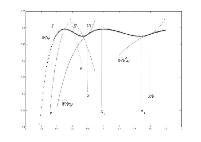
Figure 1: Graph of the Bellman function $W(x)$ (bright line with the star point markers).

On the graph, for $0<x<\bar{x}$, the Bellman function $W(x)=\tilde{W}(x)$ has three parts, denoted below as I,II and III, where it increases, strictly decreases, and again increases. Correspondingly, function $\tilde{W}(bx)$ also has three parts I,II and III where it increases, strictly decreases and increases again, and $W(x)=\tilde{W}(bx)$ for $\bar{x}\leq x<\frac{\bar{x}}{b}$. Point $\bar{x}$ is such that

$$\tilde{W}(\bar{x})=\tilde{W}(b\bar{x})\leavevmode\nobreak\ \leavevmode\nobreak\ \mbox{ and }\leavevmode\nobreak\ \leavevmode\nobreak\ \left.\frac{d\tilde{W}(x)}{dx}\right|_{\bar{x}}=\left.\frac{d\tilde{W}(bx)}{dx}\right|_{\bar{x}}.$$ (40)

As is shown in the proof of Theorem 4, these two equations are satisfied if and only if $\bar{x}$ solves equation (4).

Let us calculate the limit of $\bar{x}$ when $\rho$ approaches zero. One can easily show that, for any $x>0$,

$$\lim_{\rho\to 0}H(x)=0\leavevmode\nobreak\ \leavevmode\nobreak\ \mbox{ and }\leavevmode\nobreak\ \leavevmode\nobreak\ \lim_{\rho\to 0}\frac{H(x)}{\rho}=\frac{x^{2}(1-b)}{a}\left[\frac{\lambda(b^{2}-1)}{2}+\frac{x^{-\alpha}(1-b^{2-\alpha})}{2-\alpha}\right].$$

Let

$$\bar{x}_{0}=\left[\frac{2(1-b^{2-\alpha})}{\lambda(1-b^{2})(2-\alpha)}\right]^{1/\alpha},$$ (41)

i.e.

$$\lim_{\rho\to 0}\frac{H(x)}{\rho}\left\{\begin{array}[]{cl}>0,&\mbox{ if }x<\bar{x}_{0},\\ <0,&\mbox{ if }x>\bar{x}_{0},\\ =0,&\mbox{ if }x=\bar{x}_{0}.\end{array}\right.$$

Function $\frac{H(x)}{\rho}$ is continuous wrt $\rho$. Therefore, for any small enough $\varepsilon>0$,

$$\exists\delta>0:\leavevmode\nobreak\ \forall\rho\in(0,\delta)\leavevmode\nobreak\ \leavevmode\nobreak\ \frac{H(\bar{x}_{0}-\varepsilon)}{\rho}>0\leavevmode\nobreak\ \leavevmode\nobreak\ \mbox{ and }\leavevmode\nobreak\ \leavevmode\nobreak\ \frac{H(\bar{x}_{0}+\varepsilon)}{\rho}<0$$

meaning that $\bar{x}_{\rho}$, the solution to (4) at $\rho\in(0,\delta)$, satisfies $\bar{x}_{\rho}\in(\bar{x}_{0}-\varepsilon,\bar{x}_{0}+\varepsilon)$. This means $\lim_{\rho\to 0+}\bar{x}_{\rho}=\bar{x}_{0}$. Note that (41) is the optimal threshold if we consider the long-run average reward with the same reward rate $c(x)$.

Proof of Theorem 4.

Proof 4

(a) Firstly, let us prove that no more than one positive number $\bar{x}$ can satisfy equations (40). If $\bar{x}$ satisfies (40) then function $\tilde{W}$ canot have only one increasing branch above function $v$ because two increasing functions $\tilde{W}(x)$ and $\tilde{W}(bx)$ cannot have common points.

The increasing part I of function $\tilde{W}(x)$ cannot intersect with $\tilde{W}(bx)$.

The strictly decreasing part II of function $\tilde{W}(x)$ cannot intersect with the parts II and III of function $\tilde{W}(bx)$. Possible common points with the part I of $\tilde{W}(bx)$ are of no interest because here $\frac{d\tilde{W}(x)}{dx}<0$ and $\frac{d\tilde{W}(bx)}{dx}\geq 0$.

The increasing part III of function $\tilde{W}(x)$ can intersect with the parts I and II of function $\tilde{W}(bx)$, but again the latter case is of no interest because here $\frac{d\tilde{W}(x)}{dx}\geq 0$ and $\frac{d\tilde{W}(bx)}{dx}<0$.

Thus, the only possibility to satisfy (40) is the case when the increasing part III of $\tilde{W}(x)$ touches the increasing part I of function $\tilde{W}(bx)$. The inflection line $v(x)$ is located between the increasing and decreasing branches of the function $z(x)$, so that the part III of $\tilde{W}(x)$ is convex and the part I of $\tilde{W}(bx)$ is concave, meaning that no more than one point $\bar{x}$ can satsify the equations (40).

Using formula (34), the equations (40) can be rewritten as follows:

(42)

After we multiply these equations by factors $\left(1-be^{(b-1)\frac{\rho x}{a}}\right)$ and $\frac{a}{\rho}\left(1-e^{(b-1)\frac{\rho x}{a}}\right)$ correspondingly and subtract the equations, the variable $\tilde{w}_{1}$ is cancelled and we obtain equation

$$0 = \left(1-be^{(b-1)\frac{\rho x}{a}}\right)\left[\frac{b^{1-\alpha}x^{1-\alpha}}{\rho(\alpha-1)}+\frac{e^{\frac{b\rho x}{a}}}{\rho}\int_{x}^{bx}e^{\frac{-\rho u}{a}}u^{-\alpha}du-\frac{x^{1-\alpha}}{\rho(\alpha-1)}-(1-b)\frac{\lambda x}{\rho}\right]$$

$$-\frac{a}{\rho}\left(1-e^{\frac{(b-1)\rho x}{a}}\right)\left[\frac{be^{\frac{b\rho x}{a}}}{a}\int_{x}^{bx}e^{-\frac{\rho u}{a}}u^{-\alpha}du-(1-b)\frac{\lambda}{\rho}\right]$$

which is equivalent to $H(x)=0$.

Equation (4) follows directly from the first of equations (42): if we know the value of $x$ (equal $\bar{x}$), we can compute the value of $\tilde{w}_{1}=w_{1}$.

To prove the solvability of the equation (4) we compute the following limits:

$$\lim_{x\to\infty}H(x) \leq -\lim_{x\to\infty}e^{\frac{\rho x(1-b)}{a}}\cdot\lambda x(1-b)=-\infty;$$

$$\lim_{x\to 0}H(x) = \lim_{x\to 0}(b-1)\left[\frac{x^{1-\alpha}(1-b^{1-\alpha})}{\alpha-1}+\int_{bx}^{x}e^{-\frac{\rho u}{a}}u^{-\alpha}du\right],$$

and the positive expression in the square brackets does not exceed

$$\frac{x^{1-\alpha}(1-b^{1-\alpha})}{\alpha-1}+\int_{bx}^{x}\left[1-\frac{\rho u}{a}+\frac{1}{2}\left(\frac{\rho u}{a}\right)^{2}\right]u^{-\alpha}du=\frac{x^{1-\alpha}(1-b^{1-\alpha})}{\alpha-1}$$

$$+\left[\frac{u^{1-\alpha}}{1-\alpha}-\frac{\rho u^{2-\alpha}}{a(2-\alpha)}+\frac{\rho^{2}u^{3-\alpha}}{2a^{2}(3-\alpha)}\right]_{bx}^{x}=\left[\frac{\rho^{2}u^{3-\alpha}}{2a^{2}(3-\alpha)}-\frac{\rho u^{2-\alpha}}{a(2-\alpha)}\right]_{bx}^{x}\to 0\mbox{ as }x\to 0,$$

so that $\lim_{x\to 0}H(x)=0$.

Finally,

$$\frac{dH}{dx} = -\frac{\rho(1-b)}{a}e^{\frac{\rho x(1-b)}{a}}\left[\frac{x^{1-\alpha}(1-b^{1-\alpha})}{\alpha-1}+\lambda x(1-b)\right]$$

$$+\left(b-e^{\frac{\rho x(1-b)}{a}}\right)\left[\lambda(1-b)-x^{-\alpha}(1-b^{1-\alpha})\right]+\lambda(1-b)^{2}e^{\frac{\rho x(1-b)}{a}}$$

$$-\frac{\rho}{a}(1-b)e^{\frac{\rho x}{a}}\int_{bx}^{x}e^{-\frac{\rho u}{a}}u^{-\alpha}du-(1-b)e^{\frac{\rho x}{a}}\left[e^{-\frac{\rho x}{a}}x^{-\alpha}-be^{-\frac{\rho bx}{a}}(bx)^{-\alpha}\right]$$

$$= -\frac{\rho(1-b)(1-b^{1-\alpha})}{a(\alpha-1)}x^{1-\alpha}-\left(b-1-\frac{\rho x(1-b)}{a}\right)\left[(1-b^{1-\alpha})x^{-\alpha}-\lambda(1-b)\right]$$

$$+\lambda(1-b)^{2}-\frac{\rho}{a}(1-b)\frac{x^{1-\alpha}(1-b^{1-\alpha})}{1-\alpha}$$

$$-(1-b)\left(1+\frac{\rho x}{a}\right)\left[x^{-\alpha}\left(1-\frac{\rho x}{a}\right)-b\left(1-\frac{\rho bx}{a}\right)(bx)^{-\alpha}\right]+O(x),$$

where $\lim_{x\to 0}O(1)=0$; so

$$\lim_{x\to 0}\frac{dH}{dx}=\lim_{x\to 0}\frac{\rho(1-b)(1-b^{2-\alpha})}{a}x^{1-\alpha}=+\infty$$

meaning that the continuous function $H(x)$ increases from zero when $x\approx 0$ and becomes negative for big values of $x$.

Therefore, equation (4) has a single positive solution $\bar{x}$.

(b) Item (i) of Condition 2 is obviously satisfied (${\cal D}=\emptyset$).

For Item (ii), we consider the following three cases.

($\alpha$) Let $0<x\leq\bar{x}$. The differential equation (33) holds for function $W$ on the interval $0<x<\bar{x}$. For these values of $x$,

$$\mbox{ for any }i\geq 1,\leavevmode\nobreak\ \leavevmode\nobreak\ \leavevmode\nobreak\ W(b^{i}x)<W(x).$$ (43)

To prove this, note that function $W(bx)=\tilde{W}(bx)$ is increasing (Fig,1), so that $W(bx)>W(b^{2}x)>\ldots$ . Part III of the function $W(x)$ is convex and function $\tilde{W}(bx)$ touching smoothly $W(x)$ at point $\bar{x}$, is concave, so that $W(bx)=\tilde{W}(bx)<W(x)$ here. The same inequality holds for smaller values of $x$ where $W(x)$ decreases (part II) and $W(bx)=\tilde{W}(bx)$ increases. Part I of the function $W(x)$ is obviously bigger than $W(bx)$, too. Thus the Bellman equation (32) is satisfied on the interval $0<x<\bar{x}$ and also on the interval $(0,\bar{x}]$.

($\beta$) Consider $x\in(\bar{x},\bar{x}/b]$ and denote $x_{1}$ and $x_{2}$ the points of the analytical maximum and minimum of the function $W(x)=\tilde{W}(bx)$. (See Fig.1.)

For $x\in(\bar{x},x_{1})$ the function $W(x)$ is concave; hence

$$a\left.\frac{dW}{dx}\right|_{x}<a\left.\frac{dW}{dx}\right|_{\bar{x}}=a\left.\frac{d\tilde{W}}{dx}\right|_{\bar{x}}=\rho\tilde{W}(\bar{x})-\frac{\bar{x}^{1-\alpha}}{1-\alpha}+\lambda\bar{x}=\rho[\tilde{W}(\bar{x})-z(\bar{x})].$$

(See formula (39).) Since $W(x)$ increases starting from $W(\bar{x})=\tilde{W}(\bar{x})$ and $z(x)$ decreases, we have

$$\left.\frac{dW}{dx}\right|_{x}<\rho[W(x)-z(x)]=\rho W(x)-\left(\frac{x^{1-\alpha}}{1-\alpha}-\lambda x\right),$$

and the Bellman equation (32) is satisfied because here $W(x)=\tilde{W}(bx)=W(bx)$ and $W(b^{i+1}x)<W(bx)$ for all $i\geq 1$ because of (43).

For $x\in[x_{1},x_{2}]$ we have $W(x)>z(x)$ and $a\frac{dW}{dx}\leq 0$: remember, $W(x)=\tilde{W}(bx)$ and the latter function is of type II for $x\in[x_{1},x_{2}]$. Therefore, again

$$a\frac{dW}{dx}-\rho\left[W(x)-\frac{1}{\rho}\left(\frac{x^{1-\alpha}}{1-\alpha}-\lambda x\right)\right]<0$$

and the Bellman equation (32) is satisfied.

For $x\in(x_{2},\bar{x}/b]$, we have

$$a\frac{dW}{dx}=b\left.\frac{d\tilde{W}}{dx}\right|_{bx}<\left.\frac{d\tilde{W}}{dx}\right|_{bx}$$

because function $\tilde{W}$ increases here and $b\in(0,1)$. Next,

$$\rho[W(x)-z(x)]=\rho[\tilde{W}(bx)-z(x)]>\rho[\tilde{W}(bx)-z(bx)]$$

because the function $z(x)$ decreases. Therefore,

$$a\frac{dW}{dx}-\rho[W(x)-z(x)]<\left.\frac{d\tilde{W}}{dx}\right|_{bx}-\rho[\tilde{W}(bx)-z(bx)]=0:$$

$bx\leq\bar{x}$, and, for these values, equation (33) holds. We see that the Bellman equation (32) is satisfied.

($\gamma$) Suppose

$$a\frac{dW}{dx}-\rho[W(x)-z(x)]<0\mbox{ for }x\in\left(\frac{\bar{x}}{b^{i-1}},\frac{\bar{x}}{b^{i}}\right],$$

for some natural $i\geq 1$. Then, for $x\in\left(\frac{\bar{x}}{b^{i}},\frac{\bar{x}}{b^{i+1}}\right]$, we have

$$a\frac{dW}{dx}-\rho[W(x)-z(x)]=ba\left.\frac{dW}{dx}\right|_{bx}-\rho[W(bx)-z(x)].$$

If $\left.\frac{dW}{dx}\right|_{bx}<0$ then the last expression is negative. Otherwise,

$$ba\left.\frac{dW}{dx}\right|_{bx}\leq a\left.\frac{dW}{dx}\right|_{bx}\mbox{ and }z(x)<z(bx),$$

so that

$$a\frac{dW}{dx}-\rho[W(x)-z(x)]<a\left.\frac{dW}{dx}\right|_{bx}-\rho[W(bx)-z(bx)]<0$$

by the induction supposition.

The Bellman equation (32) is satisfied for all $x>0$.

Item (iii) of condition 2 is also obviously satisfied:

$${\cal L}^{*}=[\bar{x},\infty);\leavevmode\nobreak\ \leavevmode\nobreak\ v^{f,{\cal L}^{*}}(x)=v_{i}\mbox{ if }x\in\left[\frac{\bar{x}}{b^{i-1}},\frac{\bar{x}}{b^{i}}\right).$$

(c) Note that item (iv) of Condition 2 is not satisfied. Indeed, there is an admissible control such that, on any time interval $(T-1,T]$, $x^{\pi}(t)$ is so close to zero that $e^{-\rho T}W(x^{\pi}(t))<-1$. (Remember that $\lim_{x\to 0}W(x)=-\infty$.)

Let us fix an arbitrary $x_{0}>0$ and modify the reward rate:

$$\hat{c}(x)=\left\{\begin{array}[]{ll}c(x),&\mbox{ if }x\geq\min\{x_{0},b\bar{x}\}:=\hat{x};\\ c(\hat{x}),&\mbox{ if }x<\hat{x}.\end{array}\right.$$

Note that $\hat{c}\geq c$. The function $\tilde{W}(x)$ given by (34) will change only for $x<\hat{x}\leq x_{0}$ and remains increasing in its part I, meaning that this modified function $\hat{W}$ satisfies all items (i)–(iii) of Condition 2: the proof is identical to the one presented above. But now Condition 2 (iv) is also satisfied because the function $\hat{W}$ is bounded. Therefore, according to Theorem 2, $\sup_{\pi}\hat{J}(x_{0},\pi)=\hat{W}(x_{0})=\hat{J}(x_{0},\pi^{*})$, where $\hat{J}$ corresponds to the reward rate $\hat{c}$. But

$$\sup_{\pi}{J}_{\rho}(x_{0},\pi)\leq\sup_{\pi}\hat{J}(x_{0},\pi)=\hat{W}(x_{0})=W(x_{0}),$$

and for the feedback policy $\pi^{*}$, which is independent of $x_{0}$, we have

$$W(x_{0})=\hat{W}(x_{0})=\hat{J}(x_{0},\pi^{*})={J}_{\rho}(x_{0},\pi^{*}).$$

The last equality holds because, under the feedback policy $\pi^{*}$, starting from $x_{0}$, the trajectory $x^{\pi^{*}}(t)$ satisfies $x^{\pi^{*}}(t)\geq\hat{x}$ for all $t\geq 0$, and in this region $\hat{c}=c$.

Remark 1

The above two theorems assert that if the sending rate is smaller than $\bar{x}$, then do not send any congestion notification, while if the sending rate is greater or equal to $\bar{x},$ then send (multiple, if needed) congestion notifications until the sending rate is reduced to some level below $\overline{x}$ with $\overline{x}$ given by (17) under the average criterion and by Theorem 4(a) under the discounted criterion. This defines our proposed threshold-based AQM scheme.

4 Conclusion

To sum up, in this paper, we studied optimal impulsive control problems on infinite time interval with both discounted and time average criteria. We have established Bellman equations and provided conditions for the verification of canonical triplet. Our general results are then applied to construct a novel AQM scheme, which takes into account not only the traffic transiting through the bottleneck links but also the congestion control algorithms operating at the edges of the network. We are currently working on practical aspects of the proposed scheme and its validation. Preliminary results indicate that the new scheme improves fairness significantly with respect to alternative solutions like the RED algorithm.

06902 Sophia Antipolis Cedex Inria Domaine de Voluceau - Rocquencourt BP 105 - 78153 Le Chesnay Cedex inria.fr ISSN 0249-6399