Cosmic shear full nulling: sorting out dynamics, geometry and systematics

Abstract

An explicit full nulling scheme for cosmic shear observations is presented. It makes possible the construction of shear maps from extended source distributions for which the lens distance distribution is restricted to a definite interval. Such a construction allows to build totally independent shear maps, at all scales, that can be taken advantage of to constrain background cosmological parameters and systematics using the full statistical power of cosmic shear observations. Another advantage of such construction is that, as the lens redshift distribution can be made arbitrarily narrow, scale mixing due to projection effects can be limited allowing controlled predictions on the large scale shear power spectrum from perturbation theory calculations.

1 Introduction

After first detection of cosmic shear effects by Wittman et al. (2000); Van Waerbeke et al. (2000); Bacon et al. (2000) and the results obtained in more advance surveys (such as the CFHTLS survey, Fu et al. (2008); Heymans et al. (2012)) the science domain is about to enter an era of precision of large-scale measurements with a new generation of surveys either from ground-based facilities (e.g. DES, Pan-STARRS, LSST) or space-based observatories such as EUCLID.

Concurrently, a lot of efforts have been devoted to the development of analytical methods applied to the growth of structure and in particular to the computation of power spectra beyond linear order. These methods try to improve upon standard perturbation theory calculations and aim at proposing first principle calculations of power spectra that are valid at significantly smaller scale than standard linear theory. The first significant progress in this line of calculations is the RPT proposition (Crocce & Scoccimarro, 2006) followed by the closure theory (Taruya & Hiramatsu, 2008) and the time flow equations approach proposed in Pietroni (2008). Latest propositions, namely MPTbreeze (Crocce et al., 2012) and RegPT (Taruya et al., 2012) incorporate 2-loop order calculations and are accompanied by publicly released codes. Provided calculations are confined in their validity region, predictions from such codes can be extremely accurate, at percent level. It is then natural to try to apply these predictions to cosmic shear observations. When applied to projected convergence maps however, the results are rather disappointing as projections effects tend to mix large and small scale. It then inevitably spoils the quality of the theoretical predictions.

We have identified however a way to circumvent this problem and it is based on a nulling approach, that is a method to reorganize the multi-source plane observations of cosmic shear in such a way that the redshift distribution of the sources can be manipulated at will. Nulling has been introduced in previous studies in Joachimi & Schneider (2008) as a technique to circumvent intrinsic alignment effects by making the contributions of lenses null at a given redshift. So here we adopt a slightly different point of view. The point is not so much to find ways to circumvent such effects but to propose a transformation of the data that makes possible to sort out the information content in the weak lensing observables. This will be possible if the lens distribution can be confined to a definite distance interval to avoid scale mixing. We will see that, solving this problem leads to a reorganization of the data in such a way that most of the the cross spectra identically vanish for a given choice of a redshift-distance relation. It allows us to apply perturbation calculations to analyze the data on large angular separations. The nulling property of the transformed maps opens the path to pure geometrical tests that can be done without any knowledge of small scale physics.

Note that the aim of this study is similar to that of the 3D lensing technique (e.g., Heavens 2003; Heavens et al. 2006; Kitching et al. 2011) in the sense that we are trying to extract the density fluctuations in three-dimensional wavenumber $k$ rather than the projected angular scales. Also, several papers in the literature propose methods to avoid uncertainties on small scales (Huterer & White, 2005; Kitching & Taylor, 2011). This paper presents a simple method along these directions with a weighting scheme on galaxies according to their photometric redshift.

The plan of the paper is the following. In Section 2 we present the nulling solution for a set of discrete source planes as available in numerical simulations and exploit perturbation theory calculations to predict shear map spectra and cross-spectra in this context. In Section 3 we present an alternative tomographic basis that exhibit nulling properties for continuous source distributions. In Section 4 we explore the robustness of the nulling procedure when one introduces realistic statistical errors in the determination of the photometric redshifts and when one varies the cosmological parameters. We summarize our findings in the last section.

2 The case of discrete source planes

The construction of full nulling selection function is particularly simple in case of discrete source planes. Let us then assume we have a discrete number of source planes at redshift $z_{i}$ at our disposal. In general the local convergence $\kappa$ is given by a line-of-sight integration given by (see for instance Mellier (1999))

$$\kappa = \frac{3\Omega_{0}H_{0}^{2}}{2c^{2}}\sum_{i}p_{i}\,\int_{0}^{\chi_{i}}{\rm d}\chi\ \frac{f_{\mathrm{K}}(\chi_{i}-\chi)f_{\mathrm{K}}(\chi)}{f_{\mathrm{K}}(\chi_{i})}\frac{\delta(\chi)}{a(\chi)},$$ (1)

where $\chi$ is the radial distance, $\chi_{i}$ is the radial distance to the redshift $z_{i}$, $K$ is the (constant) space curvature, $\delta(\chi)$ is the (total matter) density contrast along the line of sight, $a(\chi)$ is the expansion factor and $p_{i}$ are dimensionless weight coefficients whose values will be chosen in order to achieve the desired properties. In the above, we define the comoving angular diameter distance:

$$f_{\mathrm{K}}(\chi)\equiv\left\{\begin{array}[]{cc}\displaystyle\frac{\sin(\sqrt{K}\chi)}{\sqrt{K}}&\mathrm{for}\,\,K>0,\\ \displaystyle\chi&\mathrm{for}\,\,K=0,\\ \displaystyle\frac{\sinh(\sqrt{-K}\chi)}{\sqrt{-K}}&\mathrm{for}\,\,K<0.\end{array}\right.$$ (5)

The expression (1) can be rewritten in the following form,

$$\kappa=\frac{3\Omega_{0}H_{0}^{2}}{2c^{2}}\int_{0}^{\chi_{\infty}}{\rm d}\chi\ \frac{\delta(\chi)}{a(\chi)}\,w(\chi),$$ (6)

with

$$w(\chi)=\sum_{i,\,\chi_{i}>\chi}p_{i}\,\frac{f_{\mathrm{K}}(\chi_{i}-\chi)f_{\mathrm{K}}(\chi)}{f_{\mathrm{K}}(\chi_{i})},$$ (7)

where $\chi_{\infty}$ is the largest radial distance available and where the sum runs for source planes that are behind the lenses. The function $w(\chi)$ here encodes the distance dependent weight with which lenses along the line of sight are contributing to the projected convergence.

The problem is now to choose a set of weights $p_{i}$ in order to build shear maps with a predefined weight form, $w(\chi)$, and in case of discrete sources, in such a way that the lens distribution is confined in a finite range of distances. The mathematical solution for a set of discrete source planes turns out to be non-ambiguous and well defined.

2.1 The 3 source plane solution

To start with let us assume that we have 3 source planes at our disposal at given distances $\chi_{i}$, $i=1,3$. The expression of $w(\chi)$ can be fruitfully replaced by,

$$w(\chi) = f_{\mathrm{K}}^{2}(\chi)\left[\frac{1}{g_{\mathrm{K}}(\chi)}\sum_{i,\chi_{i}>\chi}p_{i}-\sum_{i,\chi_{i}>\chi}\frac{p_{i}}{g_{\mathrm{K}}(\chi_{i})}\right],$$ (8)

where we have introduced

$$g_{\mathrm{K}}(\chi)\equiv\left\{\begin{array}[]{cc}\displaystyle\frac{\tan(\sqrt{K}\chi)}{\sqrt{K}}&\mathrm{for}\,\,K>0,\\ \displaystyle\chi&\mathrm{for}\,\,K=0,\\ \displaystyle\frac{\tanh(\sqrt{-K}\chi)}{\sqrt{-K}}&\mathrm{for}\,\,K<0.\end{array}\right.$$ (12)

Note that this result follows from the trigonometric identity of the sine and hyperbolic sine function in equation (5).

The key remark underlying our paper is that if the weight associated with each source plane satisfies the 2 constraints,

$$\sum_{i=1}^{3}p_{i}=0,\ \ \ \sum_{i=1}^{3}\frac{p_{i}}{g_{\mathrm{K}}(\chi_{i})}=0,$$ (13)

then whenever $\chi<\chi_{1}$ we have $w(\chi)=0$ implying that the lenses all lie between $\chi_{1}$ and $\chi_{3}$. The previous conditions can be explicitly solved and one gets (to an arbitrary normalization),

$$p_{2}/p_{1}=c(2,3,1)/c(1,2,3),\quad p_{3}/p_{1}=c(3,1,2)/c(1,2,3),$$ (14)

where

$$c(i,j,k)=g_{\mathrm{K}}(\chi_{i})\Bigl{[}g_{\mathrm{K}}(\chi_{j})-g_{\mathrm{K}}(\chi_{k})\Bigr{]}.$$ (15)

Plugging this solution into equation (8), we have the weighted lens distribution:

$$w(\chi)=\left\{\begin{array}[]{cc}\displaystyle p_{1}f_{\mathrm{K}}^{2}(\chi)\left[\frac{1}{g_{\mathrm{K}}(\chi_{1})}-\frac{1}{g_{\mathrm{K}}(\chi)}\right]&\mathrm{for}\,\,\chi_{1}\leq\chi<\chi_{2},\\ \displaystyle p_{3}f_{\mathrm{K}}^{2}(\chi)\left[\frac{1}{g_{\mathrm{K}}(\chi)}-\frac{1}{g_{\mathrm{K}}(\chi_{3})}\right]&\mathrm{for}\,\,\chi_{2}\leq\chi<\chi_{3},\\ \displaystyle 0&\mathrm{otherwise}.\end{array}\right.$$ (19)

The solution for the nulling condition is no longer unique when we have more than three source planes. However, as discussed in the next section, we can still use equation (14) with three different indices chosen arbitrarily from the available source planes even in that case to construct nulling profiles. The general solution can be obtained by taking the linear combinations of the three-plane solution (14) for different sets of planes.

2.2 Resulting correlation structure for a set of discrete planes

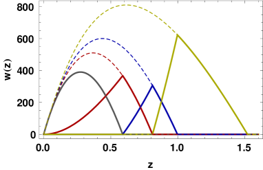
Figure 1: Shape of the lens distribution $\tilde{w}_{a}(z)$ constructed from four lens planes with the weights of Eq. (29) corresponding to the simulation of Sato et al. (2009) with $a=1$ to $4$ from left to right (see section 2.2 for detail). The lens redshift distributions $\tilde{w}_{a}(z)$ and $\tilde{w}_{b}(z)$ do not overlap when $|a-b|\geq 2$. Note that the y-axis is shown in unit of $h^{-1}\mathrm{Mpc}$.

If we have a larger set of discrete planes we can define an ordered set of source distributions for which the resulting cosmic shear maps are correlated only to their nearest ones. So let us consider a set of $n$ discrete source planes $\kappa_{i}$ located at $\chi_{i}$ where $i=1,2,\dots,n$ and $\chi_{i}<\chi_{i+1}$. One can define the $n$ maps $\tilde{\kappa}_{a}$ by taking linear combinations of the original maps $\kappa_{i}$,

$$\tilde{\kappa}_{a}=\sum_{i}p_{a}^{i}\ \kappa_{i}.$$ (20)

We can pick three neighboring lens planes and apply the three-lens solution (14) to have a nulling profile. We can construct $(n-2)$ new maps with nulling implemented by doing this to every set of three neighboring planes. We label them as $\tilde{\kappa}_{a}$ with $a\geq 3$, and these maps are nonzero between $\chi_{a-2}<\chi<\chi_{a}$. We add two more maps, $\tilde{\kappa}_{1}=\kappa_{1}$ and $\tilde{\kappa}_{2}=\kappa_{2}-\kappa_{1}$, to have a complete set of planes without loosing any information in the original $n$ planes (i.e., the matrix $p_{a}^{i}$ is invertible). Note that these two planes have nonzero lensing response down to $z=0$ as we do not apply the nulling condition to them. With this labeling convention, we have $n$ new maps $\tilde{\kappa}_{a}$, whose covering redshift ranges are in ascending order of $a$.

To summarize, the non zero coefficients are given by ,

$$p^{1}_{1}=1,\qquad p^{1}_{2}=-1,\qquad p^{2}_{2}=1,$$ (21)

for the first two maps ($a=1$ and $2$), and the remaining maps $\tilde{\kappa}_{a\geq 3}$ are given by

$$p^{a}_{a} = 1,$$ (22)

$$p^{a-1}_{a} = c(a-1,a-2,a)/c(a-2,a,a-1),$$ (23)

$$p^{a-2}_{a} = c(a-2,a-1,a)/c(a-2,a,a-1),$$ (24)

where $c(i,j,k)$ is defined in Eq. (15). It is important to note that this transformation of the $\kappa_{i}$ maps into $\tilde{\kappa}_{a}$ maps is regular. As a consequence, it does not change their information content. What we have gained here, as we will illustrate in the following, is to partially sort out the information content of the maps. It is done in two ways,

• starting with $a=3$ the maps are built out of a finite range in redshift;

• the lens distributions for $\tilde{\kappa}_{a}$ and $\tilde{\kappa}_{a+2}$ do not overlap.

We can illustrate this construction with a simple example we will exploit in the following to compare our results with numerical simulations. Using the simulations provided by Sato et al. (2009), we can exploit up to six source planes but will restrict our analysis here to the first four at $z=0.589,\ 0.811,\ 0.999$ and $1.52$ (just in order to be realistic). For a flat universe with $\Omega_{0}=0.238$, the distances to the source planes are $\chi=0.520,\ 0.680,0.800$ and $1.080$ in units of $c/H_{0}$. The resulting weight matrix reads,

$$p_{a}^{i}=\left(\begin{array}[]{cccc}1&0&0&0\\ -1&1&0&0\\ 0.4875&-1.4875&1&0\\ 0&1.46911&-2.46911&1\end{array}\right)$$ (29)

and the resulting lens weight function $\tilde{w}_{a}(z)$ are shown on Fig. 1 (solid lines). We also show the original profiles in dashed line before implementing nulling. Two such resulting convergence maps with indices that differ by more than 2 are, to systematic error effects, totally independent.

2.3 Predictions from Perturbation Theory calculations

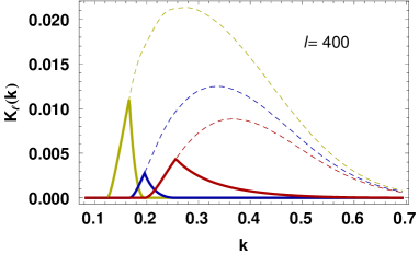
Figure 2: The kernel ${\cal K}_{\ell}(k)$ defined in Eq. (31) showing the contributing values of $k$ for $\ell=400$ for the profiles 2 to 4 (same color coding as on Fig. 1). The solid lines are for the nulling profiles and the dashed lines are for the corresponding source planes without nulling. Note that the y-axis is shown in unit of $h\,\mathrm{Mpc}^{-1}$.

We have reached here the original goal of this construction as the mapping between $\ell$ and $k$ values is now much better behaved than in standard tomographic approaches. This is illustrated on Fig. 2 (the precise definition of the kernels is given below) that shows that the contribution to $C_{\ell}$ for a given $\ell$ is now restricted to a finite range of $k$. We are now in position to fruitfully apply perturbation theory results to the projected convergence maps that are constructed through this procedure.

In the following we will compare results of numerical simulations with prediction of the RegPT scheme described in Taruya et al. (2012) at 1-loop and 2-loop order. We will also compare the results obtained when nulling is applied or not. The RegPT scheme is based on some resummation properties of the propagators and it is beyond the scope of this paper to give a detailed presentation of it. We refer the reader to Taruya et al. (2012) for a detailed presentation of this scheme and how it differs from other possible approaches. We simply recall that RegPT results can be reconstructed from standard PT diagrams. Each of these diagrams has a simple time dependence and the global time dependence of the power spectra can then easily be reconstructed from the results of the execution of the code RegPT (see again Taruya et al. (2012) for detail).

The $C_{\ell}^{ab}$ cross-power spectra are then computed from the relation,

$$C_{\ell}^{ab}=\int{\rm d}\chi\ {\cal K}_{\ell}\left(\frac{\ell}{f_{\mathrm{K}}(\chi)}\right),$$ (30)

with

$${\cal K}_{\ell}(k)=\frac{9\Omega_{0}^{2}H_{0}^{4}}{4c^{4}}\,P\left(k,\eta(\chi)\right)\frac{w_{a}(\chi)w_{b}(\chi)}{a(\chi)^{2}f_{\mathrm{K}}(\chi)^{2}},$$ (31)

where $w_{a}(\chi)$ and $w_{b}(\chi)$ are the lens distribution functions for the shear maps $(a)$ and $(b)$ and $P(k,\eta)$ is here the linear, 1-loop or 2-loop order RegPT power spectrum as a function of time. Figure 2 shows example of kernels in $k$ that contribute to values of $C_{\ell}$ for a given value of $\ell$ and for profiles 2, 3 and 4.

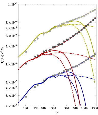
Figure 3: The resulting power spectra for the second, third and fourth bin (same color coding as on Fig. 1) when nulling is implemented. We plot the predictions of linear theory, RegPT at the 1- and 2-loop order and the revised halofit respectively by the dotted, dashed, solid and dot-dashed line, while the measurement from the simulation by Sato et al. (2009) is shown by symbols.

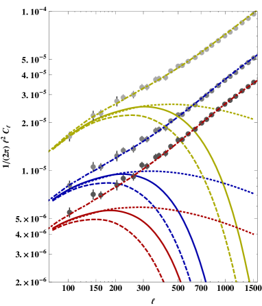
Figure 4: The resulting power spectra for the second, third and fourth source planes (same color coding as on Fig. 1) when nulling is not implemented. See text for details.

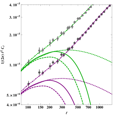
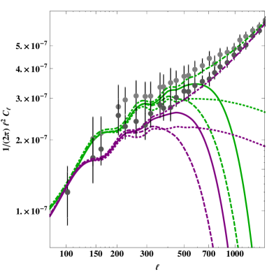
Figure 5: The resulting cross power spectra between two subsequent bins, the second and third and the third and fourth. Top panel is when no nulling is implemented and bottom panel with nulling.

We can then compute the resulting cross-spectra matrix for a set of 4 redshifts. As mentioned before, the cross-spectra matrix is band diagonal. To illustrate the performance of the computation we present the auto-correlation function for the third and fourth bin (corresponding to realistic redshift ranges) on Fig. 3. The dotted line is the linear theory, the dashed line is the 1-loop order RegPT result, the solid line is the 2-loop order RegPT result and the dot-dashed line is fitting formula for the nonlinear power spectrum (halofit: Smith et al. 2003) with revised parameters calibrated in Takahashi et al. (2012) (the revised halo fit, hereafter). Plotted in symbols are the measurements from the ray-tracing simulation by Sato et al. (2009) with error bars showing the one-$\sigma$ statistical uncertainty estimated from the scatter among the 1000 independent random realizations. We here take full advantage of the nulling prescription as it allows to extend the validity regime of perturbation theory calculations to values of $\ell$ of about 1000. This is to be compared to standard linear regime prediction which are valid to $\ell$ of about 100 as shown on Fig. 4 in the absence of nulling and for which PT predictions appear very poor because of scale mixing.

Finally in Fig. 5 we present similarly the cross-spectra between those two nearby bins (bins that are 2 indices apart exhibit of course no correlations at all). As for the auto-correlation spectra, the contribution for such cross-spectra is restricted in redshift. In all cases predictions are compared to the results of the numerical experiment of Sato et al. (2009). Note however large-scale discrepancy between the predictions and the measurements due to finite area effects (see Appendix B for detail).

Note that the revised halofit gives a good prediction over the plotted scale. This does not come as a surprise since the fitting formula is indeed calibrated by $N$-body simulations conducted with the same numerical codes with similar simulation parameters to the one shown here. Of course, further calibrations with refined simulations and eventual inclusion of possible impact of baryonic physics into the fitting formula are natural steps forward. Our strategy presented here is heading towards another direction: we are sorting out the cosmological information contents in nonlinear (complex and uncertain) regime from linear (clean and robust) regime, where the latter is accessible with perturbative techniques without free parameters or calibrations from N-body results.

3 Nulling with realistic data sets

When the sources are not confined in discrete source planes, the function $w(\chi)$, defined in eq. (7), is to be computed from a continuous source distribution,

$$w(\chi)=\int_{\chi}^{\chi_{\infty}}{\rm d}\chi_{s}p(\chi_{s})n(\chi_{s})\frac{f_{\mathrm{K}}(\chi_{s}-\chi)f_{\mathrm{K}}(\chi)}{f_{\mathrm{K}}(\chi_{s})}$$ (32)

where $\chi_{\infty}$ is the largest (finite) accessible distance to the observer and $n(\chi_{s})$ is the given distance source distribution (which can be transformed into a redshift source distribution) provided by the characteristics of the survey. Following the standard ideas of the tomographic analysis (Hu, 1999), the point is to select sources in redshift bins to gain information on the redshift evolution of clustering. In this case we can introduce the function $p(\chi_{s})$ that can then be viewed as a free parameter that the observer is free to adjust to one’s needs. The function $p(\chi_{s})$ will depend on the choices of boundaries $\chi_{1}$ and $\chi_{2}$ within which we require the lens distance to be bounded.

3.1 The multi-plane solution and the continuous limit

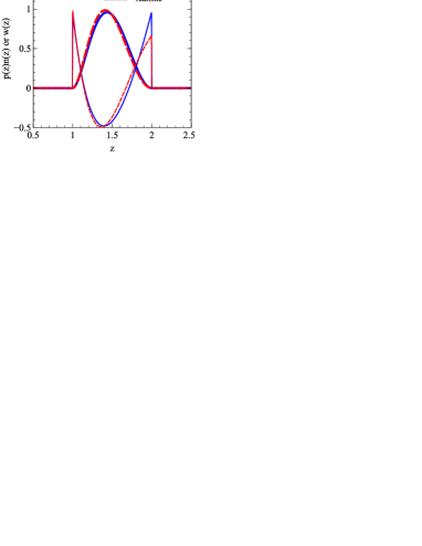
Figure 6: Example of source number density profiles (thin lines) and corresponding lens profiles (thick lines) constructed over a redshift interval of $1<z<2$. The solid (blue) lines correspond to the solution (40) in case of a constant source number density, while the dashed (red) lines show the results for $n(z)$ in Eq. (44). Note that $p(z)n(z)$ ($w(z)$) has a dimension of 1/length (length), and their normalization can be taken arbitrary.

The constraints for $p(\chi)$, that we note $p(\chi_{s};\chi_{1},\chi_{2})$ in the following, one wishes to satisfy are then the following,

$$\int_{\chi_{1}}^{\chi_{2}}{\rm d}\chi_{s}p(\chi_{s};\chi_{1},\chi_{2})n(\chi_{s}) = 0,$$ (33)

$$\int_{\chi_{1}}^{\chi_{2}}{\rm d}\chi_{s}\frac{p(\chi_{s};\chi_{1},\chi_{2})n(\chi_{s})}{g_{\mathrm{K}}(\chi_{s})} = 0$$ (34)

in order to meet the requested constraints. The difference between the discrete case is that there is a whole set of continuous solutions to this system. Further constraints should then be imposed in order to obtain a well defined solution and the natural constraint to put is to maximize the signal to noise. In particular we do not want the resulting lens selection function to be too much oscillatory making the signal small and the noise too large. The key is then to define a realistic prescription for the signal to noise. While the noise can be determined for a given survey setting (the galaxy redshift distribution, more specifically), the signal can in principle freely be designed depending on the scale of interest and the statistical quantity one considers. Thus, a fully valid prescription is non trivial in the sense that it should make intervene the nonlinear growth of perturbation which in turn is scale dependent (see Appendix A for some example prescriptions taking account of the nonlinear growth).

A simple prescription is to assume that the density contrast is simply a factor that grows like the expansion factor $a(\chi)$. In this case, the convergence field scales as (see Eq. 1)

$${\cal S}_{1} \propto \int_{0}^{\chi_{\infty}}{\rm d}\chi\,w(\chi),$$ (35)

$$= \int_{\chi_{1}}^{\chi_{2}}{\rm d}\chi_{s}p(\chi_{s})n(\chi_{s})\int_{0}^{\chi_{s}}{\rm d}\chi\frac{f_{\mathrm{K}}(\chi_{s}-\chi)f_{\mathrm{K}}(\chi)}{f_{\mathrm{K}}(\chi_{s})},$$

independently of the multipole. We adopt ${\cal S}_{1}$ as a simple estimate of the signal in the optimization. Note that the $\chi$-integral can analytically be done and the result depends on the sign of the curvature. As for the noise, we adopt the scaling

$${\cal N}^{2}\propto\int_{\chi_{1}}^{\chi_{2}}{\rm d}\chi_{s}\,p^{2}(\chi_{s})n(\chi_{s}),$$ (36)

which refers to the intrinsic shape noise contamination to the power spectrum. With these expressions for the signal and the noise, one can find explicit forms for $p(\chi)$ that satisfies the constraints (33) and (34) and maximize the signal to noise ratio for a flat universe. The ratio, which we denote by ${\cal R}$, can be rewritten in a simple form:

$${\cal R}=\frac{{\cal S}_{1}}{{\cal N}}\propto\frac{\left(p\cdot\chi^{2}\right)}{\left(p\cdot p\right)^{1/2}},$$ (37)

where we denote a scalar product of functions by

$$\left(g_{1}\cdot g_{2}\right)\equiv\int_{\chi_{1}}^{\chi_{2}}n(\chi){\rm d}\chi\,g_{1}(\chi)g_{2}(\chi).$$ (38)

The constraints (33, 34) now take the form,

$$\left(p\cdot 1\right)=0,\ \ \left(p\cdot 1/\chi\right)=0.$$ (39)

Maximizing ${\cal R}$ amounts then to find the function $p(\chi)$ in the subspace orthogonal to $m_{0}$ and $m_{-1}$ with the largest possible component along $m_{2}$, where $m_{i}=(p\cdot\chi^{i})/(p\cdot p)^{1/2}$. The solution is obtained as the result of a simple projection operator. More specifically the resulting source plane distribution takes the form (again, to an arbitrary normalization),

$$p(\chi;\chi_{1},\chi_{2})=\frac{1}{\chi_{1}\chi_{2}}\left[p_{2}(\chi)-\frac{\left(p_{2}\cdot 1/\chi\right)}{\left(1/\chi\cdot 1/\chi\right)}\ p_{-1}(\chi)\right],$$ (40)

where

$$p_{\alpha}(\chi)=\chi^{\alpha}-\frac{\left(\chi^{\alpha}\cdot 1\right)}{\left(1\cdot 1\right)}.$$ (41)

An explicit solution can be found if the available source distribution $n(\chi)$ is flat. It is then given by,

$$p(\chi;\chi_{1},\chi_{2}) = \frac{\chi^{2}}{\chi_{1}\chi_{2}}-\frac{1}{3}\left(\frac{\chi_{1}}{\chi_{2}}+\frac{\chi_{2}}{\chi_{1}}+1\right)$$ (42)

$$-\frac{1}{6}\left(\frac{\chi_{2}-\chi_{1}}{\chi}+\log\left(\chi_{2}/\chi_{1}\right)\right)$$

$$\times{\left[3\left(\frac{\chi_{2}}{\chi_{1}}-\frac{\chi_{1}}{\chi_{2}}\right)-2\left(\frac{\chi_{1}}{\chi_{2}}+\frac{\chi_{2}}{\chi_{1}}+1\right)\log\left(\frac{\chi_{2}}{\chi_{1}}\right)\right]}$$

$$/\,\left[\left(\frac{\chi_{1}}{\chi_{2}}+\frac{\chi_{2}}{\chi_{1}}-2\right)-\left(\log\left(\frac{\chi_{2}}{\chi_{1}}\right)\right)^{2}\right].$$

We show in Fig. 6, the resulting form of the weighted source distribution $p(\chi)n(\chi)$ and the lens distribution $w(\chi)$ as a function of redshift (solid lines). We also plot the solution (40) as well as the corresponding lens distribution by dashed lines when a realistic redshift distribution of source galaxies is adopted (see Eq. 44 below). The shape of the weighted source distribution is very similar in the two cases and is regular enough to be constructible from actual source distribution. Note though that it exhibits sharp features, discontinuities at the both ends, $\chi_{s}=\chi_{1}$ and $\chi_{s}=\chi_{2}$. In the case with a realistic source distribution the distribution at high redshift ($z\sim 2$) is smaller than in the constant case, reflecting the fact that the (unweighted) source number density is a decreasing function of $z$ over this redshift range. If one overweights the high-$z$ end, the resultant shape noise becomes relatively more important in the constructed map. Our signal-to-noise maximization scheme works in this way and therefore controls the relative weight around the high- and low-redshift ends.

We can choose different signal-to-noise prescriptions to determine the shape of the weight function that satisfies Eqs. (33) and (34). Although one cannot express the solution analytically in general, one still can solve them numerically with a reasonable choice of prescription. We explore some other prescriptions and summarize the results in Appendix A. Since it turns out that the resultant weight function is not very sensitive to the prescription of the signal to noise, we simply adopt Eq. (40) in what follows.

3.2 Construction of a basis of source planes

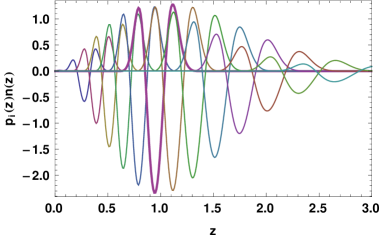
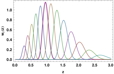
Figure 7: The adopted profiles in redshifts for the sources (top panel) and the resulting profiles for the lens distribution (bottom panel) for the fiducial cosmological model. The profiles for the sources have been obtained from the form (40) after they are convolved with a kernel that mimic the photometric redshifts error distribution. Note that $p_{i}(z)n(z)$ ($w_{i}(z)$) has a dimension of 1/length (length), and their normalization can be taken arbitrary.

The previous construction is still artificial in the sense that it assumes an infinite number of tracers. For realistic data sets, one should take into account not only the continuous nature of the source distribution but also the finite number of sources and the errors in the redshift determination. As a result it is clearly illusory to define arbitrarily narrow source distribution nor source distributions with too sharp features. It is possible however to obtain smooth source distributions from superpositions of $p(\chi_{s},\chi_{1},\chi_{2})$ taking advantage of the linearity of the constraints (33-34). As a consequence, one can convolve $p(\chi_{s},\chi_{1},\chi_{1}+\Delta\chi_{1})$ with any kernel function ${\cal G}(\chi_{1}\!-\!\chi^{\prime}_{1})$ broader or of width comparable to the typical expected error distribution in the distance. We can then build a set of profiles as

$$p_{\rm eff.}(\chi_{s};\chi_{1},\chi_{1}+\Delta\chi_{1}) =$$ (43)

$$\int{\rm d}\chi^{\prime}_{1}\,p(\chi,\chi^{\prime}_{1},\chi^{\prime}_{1}+\Delta\chi_{1})\ {\cal G}(\chi_{1}\!-\!\chi^{\prime}_{1}).$$

with arbitrary values for $\chi_{1}$ and $\Delta\chi_{1}$ that determine respectively the overall distance to the sources and its width. By linearity, the resulting shape preserves the nulling property of the original distribution. An example of such a profile is presented on Fig. 7, top panel thick line, with the corresponding lens distribution (bottom panel, thick line) where we use for ${\cal G}(\chi_{1}\!-\!\chi^{\prime}_{1})$ a kernel that corresponds to a $(1+z)3\%$ dispersion in the redshift determinations.

It is possible to vary $\chi_{1}$ to build a whole set of nulling functions that can form a basis on which to analyze the data. We propose on Fig. 7 an explicit construction of such functions. Here we assume for the total source distribution,

$$n(z)\sim(z/z_{0})^{2}\exp[-(z/z_{0})^{1.5}]$$ (44)

with $z_{0}=0.8$. The functions are regularly spaced in radial distances, i.e. $\chi_{i}=(0.05+i)c/H_{0}$ for $i=1,13$ and $\Delta\chi_{1}=0.2\ c/H_{0}$. They are found to be smooth enough to be constructible from a realistic $z$ distribution. The nulling property for this choice of functions is clearly visible on the bottom panel as the lens distributions are seen to be restricted into definite intervals.

Clearly such functions can serve as a basis for the source profiles. It can indeed be used to reconstruct any source distribution with the observed redshift resolution. One can then replace standard tomographic binning by a finite set of such functions with no loss of information. We leave for further studies the description of an optimal choice of basis.

4 Implications

4.1 Accuracy of nulling in realistic situations

There are two sources that in practice prevent us from a perfect nulling. Firstly, any dispersion of the photometric redshift widens the lensing profile as we have already discussed. Secondly, nulling requires the background geometry of the universe between the source galaxies and us to be known as an incorrect assumption in the cosmological model leads to a failed nulling profile. In this subsection, we quantify the imperfectness of nulling from these two effects employing two adjacent profiles which do not overlap when the nulling is perfect, and discuss the requirements to achieve successful nulling properties.

We consider a redshift interval of $1<z<2$ and implement nulling to the source galaxies in this (photometric) redshift range with various assumptions. We consider the source distribution function given by Eq. (44), and adopt Eq. (40) to construct a smooth profile. If nulling is implemented successfully, the resulting lensing profile should be consistent with zero at lower redshifts (i.e., $z<1$). We prepare another profile to cover $0<z<1$ and check whether the nulled profile really does not respond to the structure between the observer and $z=1$ by taking the cross correlation of the two profiles. We construct the second profile by giving a uniform weight over the source galaxies at $z<1$ for simplicity.

The weighted source number density, $p_{\mathrm{eff}}(z)n(z)$, for the two profiles are shown in the top panel of Fig. 8 when the dispersion of the photometric redshift is given by $\sigma_{z}(z)=\sigma_{0}(1+z)$ with various values of $\sigma_{0}$ assuming a Gaussian photometric redshift distribution; $\sigma_{0}=0$, $0.03$, $0.06$, $0.09$ and $0.12$ for solid, dashed, dotted dot-dashed dot-dot-dashed line, respectively. We plot the profile implementing nulling by thick lines while the other profile covering $0<z<1$ is depicted by thin lines. Note that the distribution of the photometric redshift can be much more complicated in reality with e.g., catastrophic errors or redshift dependent dispersion. The bottom panel shows the lensing profile $w$ (see equation 32 for the definition) corresponding to the source distribution in the top panel in the same line type. The two profiles approach zero at $z=1$ when we do not consider the dispersion in photo-$z$ (i.e., $\sigma_{0}=0$; solid). For increasing the value of $\sigma_{0}$, the overlap between the two becomes significant.

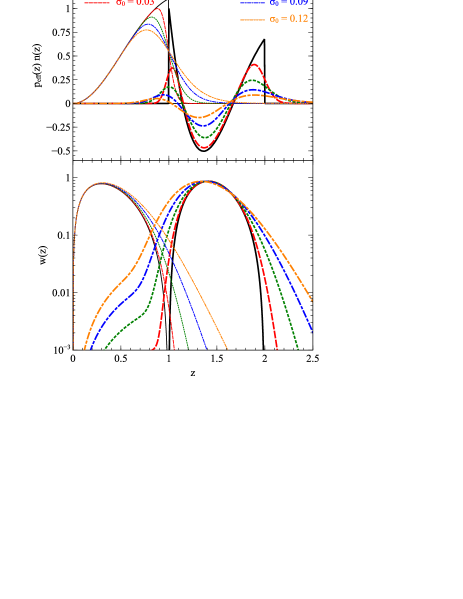
Figure 8: Effect of the dispersion of the photometric redshifts on the nulling. Two adjacent profiles (thin: $0<z<1$, thick: $1<z<2$) are plotted for different values of the dispersion parameter, $\sigma_{0}$, as shown in the legend. We plot the weighted number density of source galaxies (top panel) and the resultant lensing profile (bottom). Note that $p_{\mathrm{eft}}(z)n(z)$ ($w(z)$) has a dimension of 1/length (length), and their normalization can be taken arbitrary.

In order to quantify this overlap, we compute the cross power spectrum between the two profiles. Since the cross spectrum is expected to be zero in the ideal situation of $\sigma_{0}=0$, it provides us a measure of the accuracy of nulling. It is convenient to introduce the cross correlation coefficient between the two profiles:

$$r_{\ell}^{12}=\frac{C_{\ell}^{12}}{\sqrt{C_{\ell}^{11}C_{\ell}^{22}}}.$$ (45)

Although $C_{\ell}^{12}$ itself is dependent on the normalization of the weight functions $p_{1}(z)$ and $p_{2}(z)$, which can be chosen arbitrarily, the coefficient $r_{\ell}^{12}$ is not and it quantifies the relative amplitude of the cross power spectrum to the auto power spectra. We show this coefficient in Fig. 9 when we adopt the same values of $\sigma_{0}$ as in Fig. 8. In computing $C_{\ell}^{ij}$, we adopt the revised halofit.

When $\sigma_{0}$ is $0.03$, which is the typical target accuracy in future projects, the coefficient is $\lower 2.15277pt\hbox{$\;\buildrel<\over{\sim}\;$}10^{-3}$. It means that most of the lensing signal from the two profiles lies in the auto power spectra with this value of $\sigma_{0}$. The coefficient can be as large as $10^{-2}$ to $10^{-1}$ when the dispersion of the photometric redshift is $\sim 10\%$ depending on the multipole $\ell$ only weakly.

For comparison, the shaded region in Fig. 9 locates the level of the expected statistical error on this coefficient, $\Delta C_{\ell}^{12}/\sqrt{C_{\ell}^{11}C_{\ell}^{22}}$, for a survey with a source number density of $n_{\mathrm{tot}}=40\,\mathrm{arcmin}^{-2}$ in a survey area of $20,000\,\mathrm{deg}^{2}$. We estimate this error from

$$[\Delta C_{\ell}^{12}]^{2} = \frac{1}{N^{\mathrm{mode}}_{\ell}}\left[(C_{\ell}^{11}+C^{11}_{\mathrm{shape}})(C_{\ell}^{22}+C^{22}_{\mathrm{shape}})\right.$$ (46)

$$\hskip 56.9055pt+\left.(C_{\ell}^{12}+C^{12}_{\mathrm{shape}})^{2}\right],$$

where $N^{\mathrm{mode}}_{\ell}$ denotes the number of modes,

$$N^{\mathrm{mode}}_{\ell}=2f_{\mathrm{sky}}(\ell+1)\Delta\ell,$$ (47)

that depends on the fraction of the observed sky $f_{\mathrm{sky}}$ and the size of the $\ell$-bin $\Delta\ell$. In the above, $C^{ij}_{\mathrm{shape}}$ denotes the shape noise power spectrum:

$$C^{ij}_{\mathrm{shape}}=\frac{\sigma^{2}_{\gamma}}{n_{\mathrm{tot}}}\int_{0}^{z_{\infty}}p_{i}(z_{p})p_{j}(z_{p})n_{p}(z_{p})\mathrm{d}z_{p},$$ (48)

where $\sigma_{\gamma}$ is the dispersion of the individual galaxy shape and $n(z_{p})$ is the normalized distribution function of the photometric redshift, that can be computed from $n(z)$ for a given $\sigma_{0}$.

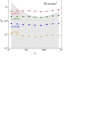
Figure 9: Cross correlation coefficient, $r_{\ell}^{12}$, for different values of the dispersion of the photometric redshifts as shown in the figure legend. The statistical error on this coefficient (i.e., the cosmic variance and the shape noise, see equation 46) is shown by the shaded region for a survey with $n_{\mathrm{tot}}=40\,\mathrm{arcmin}^{-2}$ in a area of $20,000\,\mathrm{deg}^{2}$. Note that the error level explicitly depends on the bin size of $\ell$ (see equation 46 and 47), and we adopt a logarithmic binning with three data points par decade, i.e., $\Delta\ell/\ell=0.787$. The spectra are computed using halofit formula (Smith et al., 2003) with revised parameters by Takahashi et al. (2012).

We adopt the value $\sigma_{\gamma}=0.22$ and the redshift distribution of the source in Eq. (44) in this calculation. Note that although the derivation of the formula (46) is based on the Gaussianity of the convergence field (Feldman et al., 1994), it is still exact even when there is non-Gaussianity as long as nulling is exact. This is because the cross trispectrum of the two profiles disappears thanks to the nulling property of the one restricted in $1<z<2$. In evaluating Eq. (46), we consider only the first term. The shape noise power spectrum $C_{\mathrm{shape}}^{12}$ equals to zero, because no source galaxy is included in both the profiles regardless of the value of $\sigma_{0}$. In addition, we consider the situations where nulling is approximately implemented (i.e., $C^{12}_{\ell}\simeq 0$). Thus, the first term in Eq. (46) is dominant over the second term, and the latter can safely be neglected.

The resultant statistical error on the cross correlation coefficient, $r_{\ell}^{12}$, plotted in Fig. 9 is of the same order of magnitude as the cross correlation signal when $\sigma_{0}\simeq 0.1$. If the dispersion of the photometric redshift is unexpectedly large and is around $10\%$, our technique might be useful to detect it. For a target redshift accuracy of $\sigma_{0}=0.03$, the signal is much smaller than the error level. Provided the errors on the photometric redshift are properly controlled, one should then be able to safely implement nulling within the statistical errors of future projects.

We then turn to the discussion on the error of nulling induced by a wrong assumption in the geometry of the universe. We test the accuracy of nulling with a choice of five different cosmological models when the correct cosmology is a flat $\Lambda$CDM model with $\Omega_{\mathrm{m}}=0.279$. The five models we consider are rather extreme cases; they are listed on Fig. 10 which shows their resulting angular diameter distances as a function of redshift. We then test the accuracy of the nulling method by constructing the a priori nulling profiles assuming the various cosmological models and then examining the resulting profile in the actual cosmology. As in the previous paragraph, we use two adjacent profiles. The weighted number density of the source galaxies as well as the absolute value of the resultant lensing profile are plotted in Fig. 11. We adopt $\sigma_{0}=0.03$ for the photometric redshift dispersion in this plot. Non-negligible leakage of lensing profile can be observed at $z<1$ except for the choice of the fiducial cosmology.

We finally show in Fig. 12 the cross-correlation coefficient of the two profiles obtained with the five cosmological models. The standard CDM model gives the largest signal among the five, and is close to the noise level given by Eq. (46) with the same survey design as before. This gives a rough estimate of the upper limit of the failed nulling signal. It suggests that we can safely implement nulling with more realistic cosmological assumptions. Note however that although we cannot detect a statistically meaningful signal when we focus on each of the $\ell$-bins, we might be able to detect it by combining several bins and using multiple nulling profiles, and eventually falsify the assumed cosmological model from such a diagnosis alone. This feature can be used as a unique test of cosmology, which provides us purely geometrical constraints. A more thorough discussion of the constraining power of the cosmological models through the measurement of this failed null signal will be given elsewhere together with the optimal design of a set of profiles to cover the whole range of redshift.

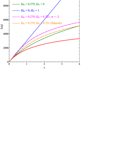
Figure 10: Comoving Angular distance in unit of $h^{-1}\mathrm{Mpc}$ as a function of redshift for five models we consider here. Matter density as well as that of cosmological constant are indicated in the labels. The model plotted in dot-dashed line considers a more general dark energy model with the equation-of-state parameter equals to $-2$, and the rest of the models are $\Lambda$CDM. Our fiducial model is shown in dot-dot-dashed line.

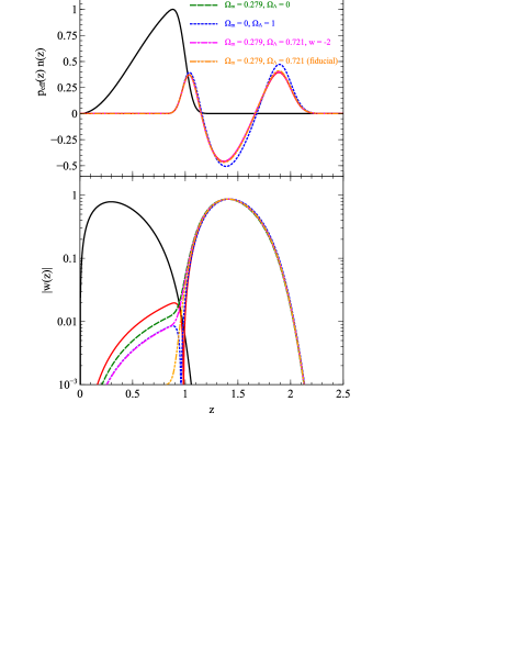
Figure 11: Effect of a wrong cosmological assumption on the nulling. Two adjacent profiles (thin: $0<z<1$, thick: $1<z<2$) are plotted for different cosmological models as shown in the legend. Top: the weighted source distribution. Bottom: the resultant lensing profile. Note that $p_{\mathrm{eft}}(z)n(z)$ ($w(z)$) has a dimension of 1/length (length), and their normalization can be taken arbitrary.

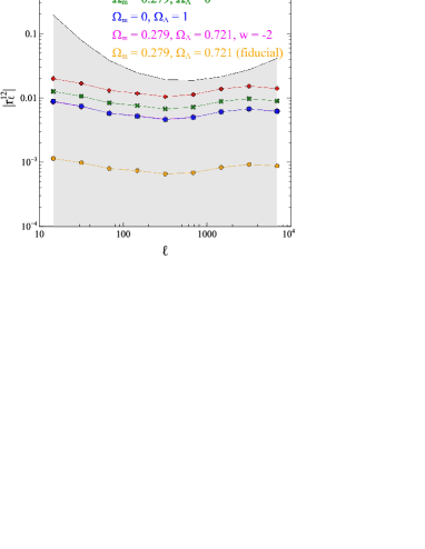
Figure 12: Cross correlation coefficient, $r_{\ell}^{12}$, when a wrong cosmological model is adopted in computing the weight function. The expected error level on $r_{\ell}^{12}$ shown in shade are the same as in Fig. 9. The spectra are computed using halofit formula (Smith et al., 2003) with revised parameters by Takahashi et al. (2012) as in Fig. 9.

4.2 Applicable range of perturbation theories

With a successful construction of the nulling lensing profile in a realistic case, we discuss here the impact of this technique on the practical application of perturbation theory, just reconsidering the results of Sec. 2.3.

For a continuous source distribution, using Eq. (40) we can construct any nulling profile with an arbitrary redshift interval. With a sufficiently large number of source galaxies, the redshift interval of the nulling profile can be made arbitrarily narrow so that the lensing kernel $w(\chi)$ is approximately described by $w(\chi)\to\delta_{\rm D}(\chi-\chi_{s})$, where $\chi_{s}$ is the radial distance to the source galaxies at redshift $z_{s}$. In this case, the multipole of the lensing power spectrum $C_{\ell}$ is directly related to the wavenumber of the three-dimensional power spectrum $P(k)$ at $z_{s}$ through

$$\ell\simeq k\,\,f_{\rm K}(\chi_{s}).$$ (49)

Thus, the accessible range of perturbation theory in $k$-space is simply mapped into the one in multipole. This is to be contrasted with the case without nulling technique. Even using source galaxies localized within an infinitesimally narrow redshift interval the contribution from the small-scale nonlinearity can affect the lensing power spectrum through the projection effect as shown in Fig. 2, shrinking the applicable range of perturbation theory.

Fig. 13 summarizes the impact of small-scale nonlinearity on the lensing power spectrum with (right) and without (left) nulling technique. The shaded colors indicate the fractional difference between nonlinear power spectrum and the perturbation theory prediction at different source redshift, $z_{s}$, as a function of multipole $\ell_{\rm lim}$. Here, we assume the best-fit Planck cosmology (Planck Collaboration, 2013) and the reference nonlinear power spectrum is computed with an updated version of the cosmic emulator code that provides interpolated power spectra from high-resolution $N$-body simulations (Heitmann et al., 2013). For perturbation theory prediction, we adopt the RegPT at two-loop order as a representative resummed PT technique (Taruya et al., 2012). We determine the wavenumber ranges of the RegPT as well as the linear theory by confronting predictions with those of the cosmic emulator. Taking advantage of the continuous source distribution, we consider the idealistic situation as discussed above, and pick up the source galaxies at arbitrary $z_{s}$ with infinitesimally thin redshift interval. In this case, with nulling technique, a simple relation with Eq. (49) may be applied to estimate the fractional discrepancy (right).

Fig. 13 clearly shows that the nulling technique is very powerful to mitigate the impact of small-scale nonlinearity. Without the nulling technique, the small-scale nonlinearities are not controlled within PT calculations, making the accessible range of RegPT results even narrower than that of the linear theory predictions (dotted and dashed lines). However, the situation is dramatically changed if we consider the nulling technique. The reliable range of RegPT predictions becomes much wider as shown by the location of the shaded areas in the right panel. The accessible range of RegPT prediction at $1\%$ precision now extends over $\ell=1300-2100$ at higher source redshift $z_{s}=2-3$. We found that this is roughly comparable to the scale where linear theory prediction produces the $20\%$ error (dashed line). Note that with the nulling technique, even the linear theory can give a reliable prediction at $1\%$ precision (dotted line) up to $\ell=550-700$ at redshift $z_{s}=2-3$, (note that at lower redshift $z_{s}\lesssim 1.5$, as the nonlinear growth of structure deforms the BAO structure, the $1\%$ boundary line, depicted as dotted lines, is made convoluted). This is a dramatic improvement. Of course, in practice, shot-noise contribution can be large due to the finite number of source galaxies, and the lens distribution will have a finite width. Nevertheless, this simple demonstration gives us a useful and general guideline to the extent with which we can apply perturbation theory to weak lensing experiments.

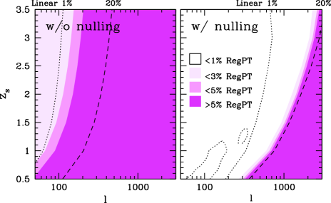
Figure 13: Impact of small-scale nonlinearity on the lensing power spectrum with (right) and without (left) nulling technique. Shaded region indicate the size of fractional difference between RegPT predictions and nonlinear power spectrum at different source redshift, $z_{s}$, plotted as a function of multipole $\ell_{\rm lim}$; $1\%$, $3\%$, and $5\%$ from lighter to darker. Here, we assume the best-fit Planck cosmology, and the reference nonlinear power spectrum is computed with an updated version of the cosmic emulator code that provides interpolated power spectra from high-resolution $N$-body simulations. We convert the results in wavenumber $k$ to those in multipole $\ell$ using Eq. (49). The dotted lines represent the locations of the $1\%$ accuracy domain of the linear theory predictions and the dashed line the $20\%$ accuracy domain. In case of nulling it approximately gives the extent of the RegPT validity domain.

5 Conclusions

We have presented a nulling construction that allows to reorganize tomographic information in such a way that different contributions to the shear maps are sorted out, geometry, systematics and regimes of dynamical evolution, a property that standard tomographic constructions does not exhibit.

After such a transformation, the correlation matrix between different maps is indeed band diagonal for all $\ell$, and most cross-correlations are nulled. This information can be exploited to all scales to constrain basic cosmological parameters, those related to the geometrical parameters. The idea we have developed here is based on the possibility of having lens distributions confined to a finite, and possibly narrow, range of redshift. Following what we have developed in the paper, such a scheme offers two advantages,

• the nulling is valid irrespectively of the regime - linear or nonlinear - and this is a key property. That means that one can use the nulling information with its full power even in regimes where exact analytic prediction are difficult;

• because one can select the redshift range of the lenses, for each chosen bin, angular scales are more closely related to physical scales making it easier to make analytical predictions. In particular because linear and nonlinear scales are not mixed up one can obtain controlled predictions to higher $\ell$ for specific source choices.

Note that in terms of amount of information there is no less and no more than with standard tomography. However the information is somehow sorted out in terms of theoretical, astrophysical and instrumental systematics. More specifically we can then put forward the part of the data that are free of theoretical uncertainties (i.e. for which one can compute exactly the statistical properties). Observed correlation when nulled signal is expected could then be used as a way to track down systematics errors such instrumental systematics (through seeing, pixellisation, masking) or astrophysical systematics through intrinsic alignment effects. Note incidentally that the fact that we have the full $\ell$ dependence of the cross-spectra should help sorting out those effects.

Furthermore the band diagonal elements themselves are better behaved in the sense that they are less sensitive to projection effects. As a result the mapping between $\ell$ and $k$ is much more precise (as illustrated on Fig. 2) making possible to associate, for each map, more closely angular scales to physical scales. And least but not last, it allows to make predictions from perturbation theory calculations to smaller angular scales, and all the more smaller that maps correspond to more distant lenses. The accuracy of such predictions are shown in Sect. 2.3. They show that analytical calculations can account of cosmic shear spectra up to $\ell$ about 1000 when lenses are at about redshift unity.

Appendix A Different prescriptions for the signal-to-noise ratio to construct continuous profiles

In the main text, we adopt Eq. (40) to obtain a smooth profile that maximizes the signal (35) with respect to the noise (36). In this Appendix, we give two alternative prescriptions for the signal to noise, and show that the resultant profiles are not sensitive to the detail of the prescription.

An alternative, and better justified approach, is to define the signal based on the significance of the power spectrum (30). Assuming that the local convergence can be estimated using the linear theory where the density power spectrum evolves linearly and scales like $a^{2}(\chi)$ and the wavenumber dependence of the three-dimensional power spectrum is effectively given by a power law with index $n$, $P(k)\propto k^{n}$, we define the signal by

$${\cal S}_{2}^{2} = \int_{0}^{\chi_{\infty}}{\rm d}\chi\,f_{\mathrm{K}}(\chi)^{-(n+2)}w^{2}(\chi),$$ (50)

where the lensing profile $w(\chi)$ is given by Eq. (32). The profiles obtained by maximization of ${\cal S}_{2}/{\cal N}$ are plotted in Fig. 14 for three values of the effective spectral index, $n=-1$, $-2$ and $-3$. The dependence of the profile on the parameter $n$ is rather weak.

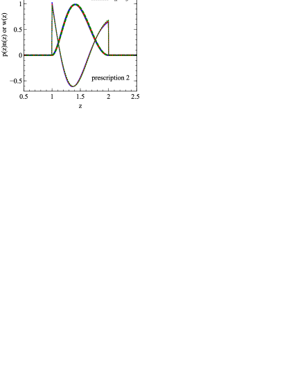
Figure 14: Nulling profiles obtained with the maximization of $({\cal S}_{2}/{\cal N})$. Note that $p(z)n(z)$ ($w(z)$) has a dimension of 1/length (length), and their normalization can be taken arbitrary.

Although it requires a model for the nonlinear power spectrum and its covariance property, we might introduce another definition of signal to noise, which is more related to the accessible information content from a power spectrum analysis. We define

$$\left(\frac{{\cal S}_{3}}{{\cal N}}\right)^{2}=\sum_{\ell,\ell^{\prime}}C_{\ell}\left(\mathrm{Cov}_{\ell\ell^{\prime}}\right)^{-1}C_{\ell^{\prime}},$$ (51)

where $\mathrm{Cov}_{\ell,\ell^{\prime}}$ denotes the covariance between $C_{\ell}$ and $C_{\ell^{\prime}}$. Assuming Gaussianity of the field $\kappa$ and for given survey parameters this reduces to

$$\left(\frac{{\cal S}_{3}}{{\cal N}}\right)^{2}=f_{\mathrm{sky}}\sum_{\ell<\ell_{\mathrm{max}}}\frac{2\ell+1}{2}\left[1+\frac{C_{\mathrm{shape}}}{C_{\ell}}\right]^{-2},$$ (52)

where we denote by $\ell_{\mathrm{max}}$ the maximum multipole taken into the summation, and the shape noise is given by

$$C_{\mathrm{shape}}=\frac{\sigma_{\gamma}^{2}}{n_{\mathrm{tot}}}\int_{\chi_{1}}^{\chi_{2}}{\rm d}\chi_{s}\,p^{2}(\chi_{s})n(\chi_{s})\propto{\cal N}^{2},$$ (53)

anologously to Eq. (48).

The resulting shape of $p(\chi_{s})$ and the lens distribution functions are shown in Fig. 15. We employ the fitting formula of the nonlinear power spectrum given by Takahashi et al. (2012) for solid and dashed line, while the linear power spectrum is used for the dashed line. Also, we adopt $\ell_{\mathrm{max}}=10,000$ except for the dashed line, which adopts $\ell_{\mathrm{max}}=1,000$. Again, we can see that the dependence of the profile on the detail of the model is rather weak.

Figure 15: Nulling profiles obtained with the maximization of $({\cal S}_{3}/{\cal N})$. Note that $p(z)n(z)$ ($w(z)$) has a dimension of 1/length (length), and their normalization can be taken arbitrary.

We finish this Appendix with a comparison of the profiles obtained with the three different prescriptions of signal to noise as shown on Fig. 16. To compute ${\cal S}_{2}$ (${\cal S}_{3}$), we adopt $n=-2$ (the nonlinear matter power spectrum up to $\ell_{\mathrm{max}}=10,000$). Notice the similarity of the profiles obtained with the maximization of ${\cal S}_{2}/{\cal N}$ and ${\cal S}_{3}/{\cal N}$. Although the prescription adopted in the main text exhibits a slightly shallower dip of the weight function at $z\sim 1.4$, the resulting profile, $w$, are almost indistinguishable.

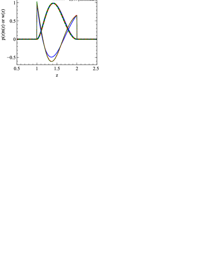
Figure 16: Comparison of the nulling profiles with different prescriptions for the signal to noise maximization. Note that $p(z)n(z)$ ($w(z)$) has a dimension of 1/length (length), and their normalization can be taken arbitrary.

Appendix B Effect of simulation window on the power spectrum measurement

In this paper, we assess the validity range of the perturbation theories by confronting it with numerical simulations. Although the analytical estimate of the nonlinear power spectrum is expected to be more accurate at larger scale (i.e., at smaller $\ell$), one may notice a slight, but statistically significant discrepancy with the numerical results at $\ell\lower 2.15277pt\hbox{$\;\buildrel<\over{\sim}\;$}200$ (see figure 3). This feature has also been reported in previous studies using the same numerical simulations (Valageas et al., 2012a, b). Since the accuracy of the models are ultimately justified by their consistency with simulations, it is important to fully understand the reason of this discrepancy.

We find out that this is likely due to the effect of finite area of ray-tracing simulations. Although the simulations we use have $25,000\,\mathrm{deg}^{2}$ in total of $1,000$ realizations, each simulated map covers only an area of $5\,\mathrm{deg}\times 5\,\mathrm{deg}$. Since one cannot mitigate the window effect by increasing the number of realizations to be averaged over, the final estimate of the power spectrum shows a slight underestimate of power at large scales comparable to the size of the each simulated convergence map.

We may write the convergence field obtained in simulations as

$$\kappa_{\mathrm{w}}(\mathbf{\theta})=\int\mathrm{d}^{2}\theta^{\prime}W(\mathbf{\theta}-\mathbf{\theta}^{\prime})\kappa(\mathbf{\theta^{\prime}}),$$ (54)

where the window function $W(\mathbf{\theta})$ is unity inside the simulation area while it is zero outside. Then the power spectrum of the windowed field, $\kappa_{\mathrm{w}}$, can be written as

$$C^{\mathrm{w}}_{\ell}=\left|\widetilde{W}(\ell)\right|^{2}C_{\ell},$$ (55)

where $\widetilde{W}$ denotes the Fourier transform of the window function $W$.

We compute the analytical power spectrum taking into account this convolution with the following procedure: we first prepare a square area of $10\,\mathrm{deg}\times 10\,\mathrm{deg}$ with periodic boundary, and generate a Gaussian random field on $256\times 256$ grid points that has the power spectrum $C_{\ell}$ computed with RegPT up to the 2-loop level. We then clip a $5\,\mathrm{deg}\times 5\,\mathrm{deg}$ region out of $10\,\mathrm{deg}\times 10\,\mathrm{deg}$, and measure the power spectrum for the clipped region. We repeat this procedure for $10,000$ times and take average of the power spectra over realizations to obtain an estimate of $C^{\mathrm{w}}_{\ell}$. We have checked that the result is stable against the area of the map in which we generate a Gaussian random field or the number of grid points.

The resultant analytical estimate is compared with simulations in Fig. 17. We here use a nulling profile constructed from the three source planes at higher redshifts by Sato et al. (2009) in order to focus on linear to weakly nonlinear regime (the exact redshifts of these source planes are $1.519$, $1.998$ and $3.057$). We plot by solid (dashed) line the RegPT prediction with (without) a convolution of the window function. The low-$\ell$ modes at $\ell\lower 2.15277pt\hbox{$\;\buildrel<\over{\sim}\;$}200$ measured from simulations (symbols with error bars) are nicely explained by the solid line while the dashed line shows a poorer fit. Another notable change induced by the convolution is the smoothed pattern of baryon acoustic oscillations seen at $300\lower 2.15277pt\hbox{$\;\buildrel<\over{\sim}\;$}\ell\lower 2.15277pt\hbox{$\;\buildrel<\over{\sim}\;$}700$. The simulation data again shows a good agreement with the solid line within the statistical error.

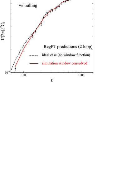
Figure 17: Comparison of the power spectrum with an without convolution of the window function.

References

- Bacon et al. (2000) Bacon D. J., Refregier A. R., Ellis R. S., 2000, Mon. Not. R. Astr. Soc. , 318, 625, arXiv:arXiv:astro-ph/0003008
- Crocce & Scoccimarro (2006) Crocce M., Scoccimarro R., 2006, Phys. Rev. D , 73, 063519, arXiv:arXiv:astro-ph/0509418
- Crocce et al. (2012) Crocce M., Scoccimarro R., Bernardeau F., 2012, Mon. Not. R. Astr. Soc. , 427, 2537, arXiv:1207.1465
- Feldman et al. (1994) Feldman H. A., Kaiser N., Peacock J. A., 1994, Astrophys. J. , 426, 23, arXiv:astro-ph/9304022
- Fu et al. (2008) Fu L., Semboloni E., Hoekstra H., Kilbinger M., et al. 2008, Astr. & Astrophys. , 479, 9, arXiv:0712.0884
- Heavens (2003) Heavens A., 2003, Mon. Not. R. Astr. Soc. , 343, 1327, arXiv:astro-ph/0304151
- Heavens et al. (2006) Heavens A. F., Kitching T. D., Taylor A. N., 2006, Mon. Not. R. Astr. Soc. , 373, 105, arXiv:astro-ph/0606568
- Heitmann et al. (2013) Heitmann K., Lawrence E., Kwan J., Habib S., Higdon D., 2013, ArXiv e-prints, arXiv:1304.7849
- Heymans et al. (2012) Heymans C. et al., 2012, Mon. Not. R. Astr. Soc. , 427, 146, arXiv:1210.0032
- Huterer & White (2005) Huterer D., White M., 2005, Phys. Rev. D , 72, 043002, arXiv:astro-ph/0501451
- Hu (1999) Hu W., 1999, Astrophys. J. Letter, 522, L21, arXiv:arXiv:astro-ph/9904153
- Joachimi & Schneider (2008) Joachimi B., Schneider P., 2008, Astr. & Astrophys. , 488, 829, arXiv:0804.2292
- Kitching & Taylor (2011) Kitching T. D., Taylor A. N., 2011, Mon. Not. R. Astr. Soc. , 416, 1717, arXiv:1012.3479
- Kitching et al. (2011) Kitching T. D., Heavens A. F., Miller L., 2011, Mon. Not. R. Astr. Soc. , 413, 2923, arXiv:1007.2953
- Laureijs et al. (2011) Laureijs R. et al., 2011, ArXiv e-prints, arXiv:1110.3193
- Mellier (1999) Mellier Y., 1999, Annual Review of Astr. & Astrophys. , 37, 127
- Pietroni (2008) Pietroni M., 2008, J. of Cosmology and Astr. Phys., 10, 36, arXiv:0806.0971
- Planck Collaboration (2013) Planck Collaboration 2013, ArXiv e-prints, arXiv:1303.5076
- Sato et al. (2009) Sato M., Hamana T., Takahashi R., Takada M., Yoshida N., Matsubara T., Sugiyama N., 2009, Astrophys. J. , 701, 945, arXiv:0906.2237
- Smith et al. (2003) Smith R. E. et al., 2003, Mon. Not. R. Astr. Soc. , 341, 1311, arXiv:astro-ph/0207664
- Takahashi et al. (2012) Takahashi R., Sato M., Nishimichi T., Taruya A., Oguri M., 2012, Astrophys. J. , 761, 152, arXiv:1208.2701
- Taruya & Hiramatsu (2008) Taruya A., Hiramatsu T., 2008, Astrophys. J. , 674, 617, arXiv:0708.1367
- Taruya et al. (2012) Taruya A., Bernardeau F., Nishimichi T., Codis S., 2012, Phys. Rev. D , 86, 103528, arXiv:1208.1191
- Valageas et al. (2012a) Valageas P., Sato M., Nishimichi T., 2012a, Astr. & Astrophys. , 541, A161, arXiv:1111.7156
- Valageas et al. (2012b) Valageas P., Sato M., Nishimichi T., 2012b, Astr. & Astrophys. , 541, A162, arXiv:1112.1495
- Van Waerbeke et al. (2000) Van Waerbeke L. et al., 2000, Astr. & Astrophys. , 358, 30, arXiv:arXiv:astro-ph/0002500
- Wittman et al. (2000) Wittman D. M., Tyson J. A., Kirkman D., Dell’Antonio I., Bernstein G., 2000, Nature , 405, 143, arXiv:arXiv:astro-ph/0003014