Modeling Limits in Hereditary Classes:
Reduction and Application to Trees

Abstract.

Limits of graphs were initiated recently in the two extreme contexts of dense and bounded degree graphs. This led to elegant limiting structures called graphons and graphings. These approach have been unified and generalized by authors in a more general setting using a combination of analytic tools and model theory to ${\rm FO}$-limits (and $X$-limits) and to the notion of modeling. The existence of modeling limits was established for sequences in a bounded degree class and, in addition, to the case of classes of trees with bounded height and of graphs with bounded tree depth. These seemingly very special classes is in fact a key step in the development of limits for more general situations. The natural obstacle for the existence of modeling limit for a monotone class of graphs is the nowhere dense property and it has been conjectured that this is a sufficient condition. Extending earlier results we derive several general results which present a realistic approach to this conjecture. As an example we then prove that the class of all finite trees admits modeling limits.

1. Introduction

The study of limiting properties of large graphs have recently received a great attention, mainly in two directions: limits of graphs with bounded degrees [1] and limit of dense graphs [11]. These developments are nicely documented in the recent monograph of Lovász [10]. Motivated by a possible unifying scheme for the study of structural limits, we introduced the notion of Stone pairing and ${\rm FO}$-convergence [16, 18]. Precisely, we proposed an approach based on the Stone pairing $\langle\phi,G\rangle$ of a first-order formula $\phi$ (with set of free variables ${\rm Fv}(\phi)$) and a graph $G$, which is defined by following expression

$$\langle\phi,G\rangle=\frac{|\{(v_{1},\dots,v_{|{\rm Fv}(\phi)|})\in G^{|{\rm Fv}(\phi)|}:G\models\phi(v_{1},\dots,v_{|{\rm Fv}(\phi)|})\}|}{|G|^{|{\rm Fv}(\phi)|}}.$$

In other words, $\langle\phi,G\rangle$ is the probability that $\phi$ is satisfied in $G$ by a random assignment of vertices (chosen independently and uniformly in the vertex set of $G$) to the free variables of $G$.

Stone pairing induces a notion of convergence: a sequence of graphs $(G_{n})_{n\in\mathbb{N}}$ is ${\rm FO}$-convergent if, for every first order formula $\phi$ (in the language of graphs), the values $\langle\phi,G_{n}\rangle$ converge as $n\rightarrow\infty$. In other words, $(G_{n})_{n\in\mathbb{N}}$ is ${\rm FO}$-convergent if the probability that a formula $\phi$ is satisfied by the graph $G_{n}$ with a random assignment of vertices of $G_{n}$ to the free variables of $\phi$ converges as $n$ grows to infinity.

It is sometimes interesting to consider weaker notions of convergence, by restricting the set of considered formulas to a fragment $X$ of ${\rm FO}$. In this case, we speak about $X$-convergence instead of ${\rm FO}$-convergence. Of special importance are the following fragments:

hv Fragment	Type of formulas	Type of convergence
vhhv ${\rm QF}$	quantifier free formulas	left convergence [11]
vhv ${\rm FO}_{0}$	sentences (no free variables)	elementary convergence
vhv ${\rm FO}_{p}$	formulas with free variables in $\{x_{1},\dots,x_{p}\}$
vhv ${\rm FO}^{\rm local}$	local formulas (depending on a fixed distance neighborhood of the free variables)
vhv ${\rm FO}_{1}^{\rm local}$	local formulas with single free variable	local convergence (if bounded degree) [1]
vh

Table 1. Fragments of specific importance.

Note that the above notions clearly extend to relational structures. Precisely, if we consider relational structures with signature $\lambda$, the symbols of the relations and constants in $\lambda$ define the non-logical symbols of the vocabulary of the first-order language ${\rm FO}(\lambda)$ associated to $\lambda$-structures. Notice that if $\lambda$ is at most countable then ${\rm FO}(\lambda)$ is countable. We have shown in [16, 18] that every finite relational structure $\mathbf{A}$ with (at most countable) signature $\lambda$ defines (injectively) a probability measure $\mu_{\mathbf{A}}$ on the standard Borel space $S(\mathcal{B}({\rm FO}(\lambda)))$, which is the Stone space of the Lindenbaum-Tarski algebra of first-order formulas (modulo logical equivalence) in the language of $\lambda$-relational structures. In this setting, a sequence $(\mathbf{A}_{n})_{n\in\mathbb{N}}$ of $\lambda$-structures is ${\rm FO}$-convergent if and only if the sequence $(\mu_{\mathbf{A}_{n}})_{n\in\mathbb{N}}$ of measures converge (in the sense of a weak-* convergence), and that the uniquely determined limit probability measure $\mu$ is such that for every first-order formula $\phi$ it holds

$$\lim_{n\rightarrow\infty}\langle\phi,\mathbf{A}_{n}\rangle=\int_{S(\mathcal{B}({\rm FO}(\lambda)))}\mathbf{1}_{K(\phi)}(T)\,{\rm d}\mu(T),$$

where $\mathbf{1}_{K(\phi)}$ stands for the indicator function of the set $K(\phi)$ of the $T\in S(\mathcal{B}({\rm FO}(\lambda)))$ such that $\phi\in T$. Note that the space of probability measures on the Stone space of a countable Boolean algebra, equipped with the weak topology, is compact.

It is natural to search for a limit object that would more look like a relational structure. Thus we introduced in [18] — as candidate for a possible limit object of sparse structures — the notion of modeling, which extends the notion of graphing introduced for bounded degree graphs. Here is an outline of its definition. A relational sample space is a relational structure $\mathbf{A}$ (with signature $\lambda$) with additional structure: The domain $A$ of $\mathbf{A}$ of a relation sample space is a standard Borel space (with Borel $\sigma$-algebra $\Sigma_{\mathbf{A}}$) with the property that every subset of $A^{p}$ that is first-order definable in ${\rm FO}(\lambda)$ is measurable (in $A^{p}$ with respect to the product $\sigma$-algebra). A modeling is a relational sample space equiped with a probability measure (denoted $\nu_{\mathbf{A}}$). For brevity we shall use the same letter $\mathbf{A}$ for structure, relational sample space, and modeling. The definition of modelings allows us to extend Stone pairing naturally to modelings: the Stone pairing $\langle\phi,\mathbf{A}\rangle$ of a first-order formula $\phi$ (with free variables in $\{x_{1},\dots,x_{p}\}$) and a modeling $\mathbf{A}$, is defined by

$$\langle\phi,\mathbf{A}\rangle=\idotsint\mathbf{1}_{\Omega_{\phi}(\mathbf{A})}(x_{1},\dots,x_{p})\,{\rm d}\nu_{\mathbf{A}}(x_{1})\dots\rm d\nu_{\mathbf{A}}(x_{p}),$$

where $\mathbf{1}_{\Omega_{\phi}(\mathbf{A})}$ is the indicator function of the solution set $\Omega_{\phi}(\mathbf{A})$ of $\phi$ in $\mathbf{A}$, that is:

$$\Omega_{\phi}(\mathbf{A})=\{(v_{1},\dots,v_{p})\in A^{p}:\quad\mathbf{A}\models\phi(v_{1},\dots,v_{p}).$$

Note that every finite structure canonically defines a modeling (with same universe, discrete $\sigma$-algebra, and uniform probability measure) and that in the definition above matches the definition of Stone pairing of a formula and a finite structure introduced earlier.

In the following, we assume that free variables of formulas are of the form $x_{i}$ with $i\in\mathbb{N}$. Note that the free variables need not to be indexed by consecutive integers. For a formula $\phi$, denote by $\phi^{\triangledown}$ the formula obtained by packing the free variables of $\phi$: if the free variables of $\phi$ are $x_{i_{1}},\dots,x_{i_{p}}$ with $i_{1}<i_{2}<\dots<i_{p}$ then $\phi^{\triangledown}$ is obtained from $\phi$ by renaming $x_{i_{1}},\dots,x_{i_{p}}$ to $x_{1},\dots,x_{p}$. Although $\Omega_{\phi}(\mathbf{A})$ and $\Omega_{\phi^{\triangledown}}(\mathbf{A})$ differ in general, it is clear that they have same measure (as $\Omega_{\phi}(\mathbf{A})$ can be obtained from $\Omega_{\phi^{\triangledown}}(\mathbf{A})$ by taking the Cartesian product by some power of $A$, and then permuting the coordinates). Hence for every formula $\phi$ it holds

$$\langle\phi,\,\cdot\,\rangle=\langle\phi^{\triangledown},\,\cdot\,\rangle,$$

that is: the Stone pairing is invariant by renaming of the free variables.

The expressive power of the Stone pairing goes slightly beyond satisfaction statistics of first-order formulas. In particular, we prove (see Corollary 1) that the Stone pairing $\langle\,\cdot\,,\mathbf{A}\rangle$ can be extended in a unique way to the infinitary language $\mathcal{L}_{\omega_{1}\omega}$, which is an extension of ${\rm FO}$ allowing countable conjunctions and disjunctions [20, 21]. Note that this language is still complete, as proved by Karp [5]. Although the compactness theorem does not hold for $\mathcal{L}_{\omega_{1},\omega}$, the interpolation theorem for $\mathcal{L}_{\omega_{1},\omega}$ was proved by Lopez-Escobar [9] and Scott’s isomorphism theorem for $\mathcal{L}_{\omega_{1},\omega}$ by Scott [19]. For a modeling $\mathbf{A}$ and an integer $p$, the $\mathcal{L}_{\omega_{1},\omega}$-definable subsets of $A^{p}$ correspond to the smallest $\sigma$-algebra that contains all the first-order definable subsets of $A^{p}$ (see Lemma 7). According to the definition of a modeling, this means that all $\mathcal{L}_{\omega_{1},\omega}$-definable sets of a modeling are Borel measurable.

We say that a class $\mathcal{C}$ of structures admits modeling limits if for every ${\rm FO}$-convergent sequence of structures $\mathbf{A}_{n}\in\mathcal{C}$ there is a modeling $\mathbf{L}$ such that for every $\phi\in{\rm FO}$ it holds

$$\langle\phi,\mathbf{L}\rangle=\lim_{n\rightarrow\infty}\langle\phi,\mathbf{A}_{n}\rangle,$$

what we denote by $\mathbf{A}_{n}\xrightarrow{\rm FO}\mathbf{L}$. More generally, for a fragment $X$ of ${\rm FO}$, we say that a class $\mathcal{C}$ of structures admits modeling $X$-limits if for every ${X}$-convergent sequence of structures $\mathbf{A}_{n}\in\mathcal{C}$ there is a modeling $\mathbf{L}$ such that for every $\phi\in X$ it holds $\langle\phi,\mathbf{L}\rangle=\lim_{n\rightarrow\infty}\langle\phi,\mathbf{A}_{n}\rangle$, and we denote this by $\mathbf{A}_{n}\xrightarrow{X}\mathbf{L}$.

The following results have been proved in [18]:

• every class of graphs with bounded degree admits modeling limits;

• every class of graphs of colored rooted trees bounded height admits modeling limits;

• every class of graphs with bounded tree-depth admits modeling limits.

On the other hand, only sparse monotone classes of graphs can admits modeling limits. Precisely, if a monotone class of graphs admits modeling limits, then it is nowhere dense [18], and we conjectured that a monotone class of graphs actually admits modeling limits if and only if it is nowhere dense.

Recall that a monotone class of graphs ${\mathcal{C}}$ is nowhere dense if, for every integer $p$ there exists a graph whose $p$-subdivision is not in $\mathcal{C}$ (for more on nowhere dense graphs, see [13, 12, 14, 15, 17]). The importance of nowhere dense classes and the strong relationship of this notion with first-order logic is examplified by the recent result of Grohe, Kreutzer, and Siebertz [4], which states that (under a reasonable complexity theoretic assumption) deciding first-order properties of graphs in a monotone class $\mathcal{C}$ is fixed-parameter tractable if and only if $\mathcal{C}$ is nowhere dense.

In this paper, we initiate a systematic study of hereditary classes that admit modeling limits. We prove that the problem of the existence of a modeling limit can be reduced to the study of ${\rm FO}^{\rm local}$-convergence, and then to two “typical” particular cases:

• Residual sequences, that is sequences such that (intuitively) the limit has only zero-measure connected components,

• Non-dispersive sequences, that is sequences such that (intuitively) the limit is (almost) connected.

A modeling $\mathbf{A}$ with universe $A$ satisfies the Finitary Mass Transport Principle if, for every $\phi,\psi\in{\rm FO}_{1}(\lambda)$ and every integers $a,b$ such that

$$\begin{cases}\phi\vdash(\exists^{\geq a}y)\,(x_{1}\sim y)\wedge\psi(y)\\ \psi\vdash(\exists^{\leq b}y)\,(x_{1}\sim y)\wedge\phi(y)\end{cases}$$

it holds

$$a\,\langle\phi,\mathbf{A}\rangle\leq b\,\langle\psi,\mathbf{A}\rangle.$$

It is clear that every finite structure satisfies the Finitary Mass Transport Principle, hence every modeling ${\rm FO}$-limit of finite structures satisfies the Finitary Mass Transport Principle, too.

A stronger version of this principle, which is also satisfied by every finite structure, does not automatically hold in the limit. A modeling $\mathbf{A}$ with universe $A$ satisfies the Strong Finitary Mass Transport Principle if, for every measurable subsets $X,Y$ of $A$, and every integers $a,b$, the following property holds:

If every $x\in X$ has at least $a$ neighbors in $Y$ and every $y\in Y$ has at most $b$ neighbors in $X$ then $a\,\nu_{\mathbf{A}}(X)\leq b\,\nu_{\mathbf{A}}(Y)$.

In this context, we prove the following theorem, which is the principal result of this paper.

Theorem 1.

Let $\mathcal{C}$ be a hereditary class of structures.

Assume that for every $\mathbf{A}_{n}\in\mathcal{C}$ and every $\rho_{n}\in A_{n}$ ($n\in\mathbb{N}$) the following properties hold:

1. if $(\mathbf{A}_{n})_{n\in\mathbb{N}}$ is ${\rm FO}_{1}^{\rm local}$-convergent and residual, then it has a modeling ${\rm FO}_{1}^{\rm local}$-limit;

2. if $(\mathbf{A}_{n},\rho_{n})_{n\in\mathbb{N}}$ is ${\rm FO}^{\rm local}$-convergent (resp. ${\rm FO}_{p}^{\rm local}$-convergent) and $\rho$-non-dispersive then it has a modeling ${\rm FO}^{\rm local}$-limit (resp. a ${\rm FO}_{p}^{\rm local}$-limit).

Then $\mathcal{C}$ admits modeling limits (resp. modeling ${\rm FO}_{p}$-limits).

Moreover, if in cases (1) and (2) the modeling limits satisfy the Strong Finitary Mass Transport Principle, then $\mathcal{C}$ admits modeling limits (resp. modeling ${\rm FO}_{p}$-limits) that satisfy the Strong Finitary Mass Transport Principle.

Then we apply this theorem in Section 8 to give a simple proof of the fact that the class of forests admit modeling limits.

Theorem 2.

The class of finite forests admits modeling limits, that is: every ${\rm FO}$-convergent sequence of finite forests as a modeling ${\rm FO}$-limit that satisfies the Strong Finitary Mass Transport Principle.

Note that a result similar to Theorem 2 was recently claimed by Kráľ, Kupec, and Tůma [7].

2. Preliminaries

Let $\mathbf{A}$ be a relational structure with signature $\lambda$ and universe $A$, and let $X\subseteq A$. The substructure $\mathbf{A}[X]$ induced by $X$ has domain $X$ and the same relations as $\mathbf{A}$ (restricted to $X$). A class $\mathcal{C}$ of $\lambda$-structures is hereditary if every induced substructure of a structure in $\mathcal{C}$ belongs to $\mathcal{C}$: $(\forall\mathbf{A}\in\mathcal{C},\forall X\subset A)\ \mathbf{A}[X]\in\mathcal{C}$.

The distance between two vertices $u,v\in A$ is the smallest number of relations inducing a connected substructure of $\mathbf{A}$ and containing both $u$ and $v$, that is the graph distance between $u$ and $v$ in the Gaifman graph of $\mathbf{A}$. For $r\in\mathbb{N}$ and $v\in A$, we denote by $B_{r}(\mathbf{A},v)$ the ball of radius $r$ centered at $v$, that is the substructure of $\mathbf{A}$ induced by the vertices at distance at most $r$ from $v$ in $\mathbf{A}$. More generally, for $v_{1},\dots,v_{k}\in A$, we denote by $B_{r}(\mathbf{A},v_{1},\dots,v_{k})$ the substructure of $\mathbf{A}$ induced by the vertices at distance at most $r$ from at least one of the $v_{i}$ ($1\leq i\leq k$) in $\mathbf{A}$.

A formula $\phi\in{\rm FO}_{p}^{\rm local}$ is $r$-local if its satisfaction only depends on the $r$-neighborhood of the free variables, that is: for every $\lambda$-structure $\mathbf{A}$ and every $v_{1},\dots,v_{p}\in A^{p}$ it holds

$$\mathbf{A}\models\phi(v_{1},\dots,v_{p})\quad\iff\quad B_{r}(\mathbf{A},v_{1},\dots,v_{p})\models\phi(v_{1},\dots,v_{p}).$$

Recall the particular case of Gaifman locality theorem for sentences, which we will be usefull in the following. A local sentence is a sentence of the form

$$\exists x_{1}\dots\exists x_{k}\ \bigl{(}\bigwedge_{1\leq i<j\leq k}{\rm dist}(x_{i},x_{j})>2r\ \wedge\ \bigwedge_{1\leq i\leq k}\psi_{i}(x_{i})\bigr{)},$$

where $r,k\geq 1$ and $\psi_{i}$ is $r$-local.

Theorem 3 (Gaifman [3]).

Every first-order sentence is equivalent to a Boolean combination of local sentences.

We end this section with two very simple but usefull lemmas.

Lemma 4.

Let $\phi,\psi$ be formulas. Then it holds

$$|\langle\phi,\,\cdot\,\rangle-\langle\phi\wedge\psi,\,\cdot\,\rangle|\leq 1-\langle\psi,\,\cdot\,\rangle.$$

Proof.

$$\langle\psi\wedge\phi,\,\cdot\,\rangle\leq\langle\phi,\,\cdot\,\rangle=\langle\neg\psi\wedge\phi,\,\cdot\,\rangle+\langle\psi\wedge\phi,\,\cdot\,\rangle\leq\langle\neg\psi,\,\cdot\,\rangle+\langle\psi\wedge\phi,\,\cdot\,\rangle,$$

Thus

$$|\langle\phi,\,\cdot\,\rangle-\langle\phi\wedge\psi,\,\cdot\,\rangle|\leq\langle\neg\psi,\,\cdot\,\rangle=1-\langle\psi,\,\cdot\,\rangle.$$

∎

Lemma 5.

Let $\psi_{1},\dots,\psi_{p}$ be formulas without common free variables. Then it holds

$$\langle\bigwedge_{i=1}^{p}\psi_{i},\,\cdot\,\rangle=\prod_{i=1}^{p}\langle\psi_{i},\,\cdot\,\rangle.$$

Proof.

Let $k=\max\{i:x_{i}\in\bigcup_{j=1}^{p}{\rm Fv}(\psi_{j})\}-\sum_{j=1}^{p}|{\rm Fv}(\psi_{j})|$. For every modeling $\mathbf{A}$, the solution set $\Omega_{\bigwedge_{i=1}^{p}\psi_{i}(x_{i})}(\mathbf{A})$ can be obtained from $\Omega_{\psi_{1}^{\triangledown}}(\mathbf{A})\times\dots\times\Omega_{\psi_{p}^{\triangledown}}(\mathbf{A})\times A^{k}$ by permuting the coordinates, hence both sets have the same measure, that is:

$$\langle\bigwedge_{i=1}^{p}\psi_{i},\,\cdot\,\rangle=\prod_{i=1}^{p}\langle\psi_{i}^{\triangledown},\,\cdot\,\rangle=\prod_{i=1}^{p}\langle\psi_{i},\,\cdot\,\rangle.$$

∎

3. What does Stone pairing measure?

By definition, the Stone pairing $\langle\phi,\mathbf{A}\rangle$ measures the probability that a given first-order formula $\phi$ is satisfied in $\mathbf{A}$ by a random assignment of vertices of $\mathbf{A}$ to the free variables. For this definition to make sense, we have to assume that every subset of a power of $A$ that is first-order definable without parameters is measurable. Hence we have to consider, for each $p\in\mathbb{N}$, a $\sigma$-algebra on $A^{p}$ that contains all subsets of $A^{p}$ that are first-order definable without parameters.

The aim of this section is to prove that the minimal $\sigma$-algebra including all subsets of $A^{p}$ that are first-order definable without parameters is exactly the family of all subsets of $A^{p}$ that are $\mathcal{L}_{\omega_{1}\omega}$-definable without parameters.

We take time out for two lemmas.

Lemma 6.

Let $\Omega$ be a set. For $p\in\mathbb{N}$, let $\mathcal{A}_{p}$ be a field of sets on $\Omega^{p}$, and let $\sigma(\mathcal{A}_{p})$ be the minimal $\sigma$-algebra that contains $\mathcal{A}_{p}$. For $p\in\mathbb{N}$, let $f_{p}:\Omega^{p+1}\rightarrow\Omega^{p}$ and let $F_{p}:\mathcal{P}(\Omega^{p+1})\rightarrow\mathcal{P}(\Omega^{p})$ be defined by $F_{p}(X)=\{f_{p}(x):x\in X\}$.

Assume that for each $p\in\mathbb{N}$, $F_{p}$ maps $\mathcal{A}_{p+1}$ to $\mathcal{A}_{p}$.

Then $F_{p}$ maps $\sigma(\mathcal{A}_{p+1})$ to $\sigma(\mathcal{A}_{p})$.

Proof.

The proof follows the standard construction of a $\sigma$-algebra by transfinite induction. For $p\in\mathbb{N}$, we let

• $\mathcal{S}_{p,0}$ be the collection of sets obtained as countable unions of increasing sets in $\mathcal{A}_{p}$, that is: sets of the form $\bigcup_{i\in\mathbb{N}}X_{i}$ where $X_{i}\in\mathcal{A}_{p}$ and $X_{1}\subseteq X_{2}\subseteq\dots\subseteq X_{n}\subseteq\dots$;

• $\mathcal{P}_{p,0}$ be the collection of sets obtained as countable intersections of decreasing sets in $\mathcal{A}_{p}$, that is: sets of the form $\bigcap_{i\in\mathbb{N}}X_{i}$ where $X_{i}\in\mathcal{A}_{p}$ and $X_{1}\supseteq X_{2}\supseteq\dots\supseteq X_{n}\supseteq\dots$;

• (for $i\geq 1$ not a limit ordinal) $\mathcal{S}_{p,i}$ be the collection of sets obtained as countable unions of increasing sets in $\mathcal{P}_{p,i-1}$;

• (for $i\geq 1$ not a limit ordinal) $\mathcal{P}_{p,i}$ be the collection of sets obtained as countable intersections of decreasing sets in $\mathcal{S}_{p,i-1}$;

• (for $i$ limit ordinal) $\mathcal{S}_{p,i}=\bigcup_{j<i}S_{p,j}$ and $\mathcal{P}_{p,i}=\bigcup_{j<i}P_{p,j}$.

Then it is easily checked that by induction that for every $i$ up to $\omega_{1}$ it holds:

• for all $X\in\Omega^{p}$, $(X\in\mathcal{S}_{p,i})\iff(\Omega^{p}\setminus X\in\mathcal{P}_{p,i})$;

• for every limit ordinal $i$, $\mathcal{S}_{p,i}=\mathcal{P}_{p,i}$;

• if $X,Y\in\mathcal{S}_{p,i}$ then $X\cup Y\in\mathcal{S}_{p,i}$ and $X\cap Y\in\mathcal{S}_{p,i}$;

• if $X,Y\in\mathcal{P}_{p,i}$ then $X\cup Y\in\mathcal{P}_{p,i}$ and $X\cap Y\in\mathcal{P}_{p,i}$;

• $F_{p}$ maps $\mathcal{S}_{p+1,i}$ to $\mathcal{S}_{p,i}$ and $\mathcal{P}_{p+1,i}$ to $\mathcal{P}_{p,i}$;

According to the monotone class theorem, $\sigma(\mathcal{A}_{p})=\mathcal{S}_{p,\omega_{1}}=\mathcal{P}_{p,\omega_{1}}$. ∎

Lemma 7.

We consider a relational structure $\mathbf{A}$ with countable signature.

Let $\mathcal{A}_{p}$ (resp. $\mathcal{A}_{p}^{+}$) be the field of sets of all the subsets of $A^{p}$ that are first-order definable without (resp. with) parameters. Then the smallest $\sigma$-algebra $\sigma(\mathcal{A}_{p})\supseteq\mathcal{A}_{p}$ (resp. $\sigma(\mathcal{A}_{p}^{+})\supseteq\mathcal{A}_{p}^{+}$) is the algebra of all the subsets of $A^{p}$ that are definable in $\mathcal{L}_{\omega_{1}\omega}$ without (resp. with) parameters.

Proof.

Let $\Omega=L$ and $f_{p}:A^{p+1}\rightarrow A^{p}$ be the projection map. According to Lemma 6, the projection map send sets in $\sigma(\mathcal{A}_{p+1})$ to sets in $\sigma(\mathcal{A}_{p})$ (and sets in $\sigma(\mathcal{A}_{p+1}^{+})$ to sets in $\sigma(\mathcal{A}_{p}^{+})$). It follows easily that subsets of $A^{p}$ that are $\mathcal{L}_{\omega_{1}\omega}$-definable without (resp. with) parameters are exactly those in $\sigma(\mathcal{A}_{p})$ (resp. $\sigma(\mathcal{A}_{p}^{+})$). ∎

Note that when $\mathbf{A}$ is a modeling, the collection of the subsets of $A^{p}$ definable in $\mathcal{L}_{\omega_{1}\omega}$ without parameters is the $\sigma$-algebra generated by the projection $\tensor*[^{p}_{\scriptscriptstyle\mathbf{A}}]{\sf\textstyle Tp}{}:A^{p}\rightarrow S(\mathcal{B}({\rm FO}_{p}))$, mapping a $p$-tuple of vertices of $A$ to its $p$-type: a subset $X$ of $A^{p}$ is definable in $\mathcal{L}_{\omega_{1}\omega}$ without parameters if and only if it is the preimage by $\tensor*[^{p}_{\scriptscriptstyle\mathbf{A}}]{\sf\textstyle Tp}{}$ of a Borel subset of $S(\mathcal{B}({\rm FO}_{p}))$ (see [18] for detailed definition and analysis of $\tensor*[^{p}_{\scriptscriptstyle\mathbf{A}}]{\sf\textstyle Tp}{}$).

Corollary 1.

For every modeling $\mathbf{A}$ the Stone pairing $\langle\,\cdot\,,\mathbf{A}\rangle$ can be extended in a unique way to $\mathcal{L}_{\omega_{1}\omega}$.

Remark 8.

Let $\Xi(\lambda)$ be the set of all probability measures on the Stone space $S(\mathcal{B}({\rm FO}(\lambda)))$, and let $\mathcal{B}$ be the $\sigma$-algebra generated by evaluation maps $\mu\mapsto\mu(A)$ for $A$ measurable set of $S(\mathcal{B}({\rm FO}(\lambda)))$. It is well known that $(\Xi(\lambda),\mathcal{B})$ is a standard Borel space ([6], Sect. $17$.E). (Hence the space of all finite $\lambda$-structures and their ${\rm FO}$-limits is also a compact standard Borel space, as it can be identified to a closed subspace of $\Xi(\lambda)$.) The mapping $\mathbf{A}\mapsto\nu_{\mathbf{A}}$ embeds the space $M$ of modelings into $\Xi(\lambda)$. The initial topology on $M$ with respect to this mapping is the same as the topology induced by Stone pairing. Hence the mapping $\langle\phi,\,\cdot\,\rangle:M\rightarrow[0,1]$, which maps $\mathbf{A}$ to $\langle\phi,\mathbf{A}\rangle$, is continuous for $\phi\in{\rm FO}(\lambda)$, and measurable for $\phi\in{\mathcal{L}_{\omega_{1}\omega}}(\lambda)$.

Also remark that the topology of $\Xi(\lambda)$ can be defined by means of Lévy–Prokhorov metric (by choosing some metric on the Stone space). For instance, for finite signature $\lambda$, the topology of $M$ can be generated by the pseudometric:

$${\rm dist}(\mathbf{A},\mathbf{B})=2^{-\sup\{n|\ \forall\phi\in{\rm FO}(\lambda),\,{\rm qrank}(\phi)+|{\rm Fv}(\phi)|\leq n\Rightarrow|\langle\phi,\mathbf{A}\rangle-\langle\phi,\mathbf{B}\rangle|<2^{-n}\}}.$$

Theorem 9.

Let $\mathbf{A}$ be a relational sample space. Then every subset of $A^{p}$ that is $\mathcal{L}_{\omega_{1}\omega}$-definable (with parameters) is measurable (with respect to product Borel $\sigma$-algebra $\Sigma_{\mathbf{A}}^{\otimes p}$).

3.1. Interpretation Schemes

Interpretation Schemes (introduced in this setting in [18]) generalize to other logics than ${\rm FO}$.

Definition 10.

Let $\mathcal{L}$ be a logic (for us, ${\rm FO}$ or ${\mathcal{L}}_{\omega_{1}\omega}$). For $p\in\mathbb{N}$ and a signature $\lambda$, $\mathcal{L}_{p}(\lambda)$ denotes the set of the formulas in the language of $\lambda$ in logic $\mathcal{L}$, with free variables in $\{x_{1},\dots,x_{p}\}$.

Let $\kappa,\lambda$ be signatures, where $\lambda$ has $q$ relational symbols $R_{1},\dots,R_{q}$ with respective arities $r_{1},\dots,r_{q}$.

An $\mathcal{L}$-interpretation scheme ${\mathsf{I}}$ of $\lambda$-structures in $\kappa$-structures is defined by an integer $k$ — the exponent of the $\mathcal{L}$-interpretation scheme — a formula $E\in{\mathcal{L}}_{2k}(\kappa)$, a formula $\theta_{0}\in{\mathcal{L}}_{k}(\kappa)$, and a formula $\theta_{i}\in{\rm FO}_{r_{i}k}(\kappa)$ for each symbol $R_{i}\in\lambda$, such that:

• the formula $E$ defines an equivalence relation of $k$-tuples;

• each formula $\theta_{i}$ is compatible with $E$, in the sense that for every $0\leq i\leq q$ it holds

  $$\bigwedge_{1\leq j\leq r_{i}}\,E(\mathbf{x}_{j},\mathbf{y}_{j})\quad\vdash\quad\theta_{i}(\mathbf{x}_{1},\dots,\mathbf{x}_{r_{i}})\leftrightarrow\theta_{i}(\mathbf{y}_{1},\dots,\mathbf{y}_{r_{i}}),$$

  where $r_{0}=1$, boldface $\mathbf{x}_{j}$ and $\mathbf{y}_{j}$ represent $k$-tuples of free variables, and where $\theta_{i}(\mathbf{x}_{1},\dots,\mathbf{x}_{r_{i}})$ stands for $\theta_{i}(x_{1,1},\dots,x_{1,k},\dots,x_{r_{i},1},\dots,x_{r_{i},k})$.

For a $\kappa$-structure $\mathbf{A}$, we denote by $\mathsf{I}(\mathbf{A})$ the $\lambda$-structure $\mathbf{B}$ defined as follows:

• the domain $B$ of $\mathbf{B}$ is the subset of the $E$-equivalence classes $[\mathbf{x}]\subseteq A^{k}$ of the tuples $\mathbf{x}=(x_{1},\dots,x_{k})$ such that $\mathbf{A}\models\theta_{0}(\mathbf{x})$;

• for each $1\leq i\leq q$ and every $\mathbf{v}_{1},\dots,\mathbf{v}_{s_{i}}\in A^{kr_{i}}$ such that $\mathbf{A}\models\theta_{0}(\mathbf{v}_{j})$ (for every $1\leq j\leq r_{i}$) it holds

  $$\mathbf{B}\models R_{i}([\mathbf{v}_{1}],\dots,[\mathbf{v}_{r_{i}}])\quad\iff\quad\mathbf{A}\models\theta_{i}(\mathbf{v}_{1},\dots,\mathbf{v}_{r_{i}}).$$

From the standard properties of model theoretical interpretations (see, for instance [8] p. 180), we state the following: if $\mathsf{I}$ is an $\mathcal{L}$-interpretation of $\lambda$-structures in $\kappa$-structures, then there exists a mapping $\tilde{\mathsf{I}}:{\mathcal{L}}(\lambda)\rightarrow{\mathcal{L}}(\kappa)$ (defined by means of the formulas $E,\theta_{0},\dots,\theta_{q}$ above) such that for every $\phi\in{\mathcal{L}}_{p}(\lambda)$, and every $\kappa$-structure $\mathbf{A}$, the following property holds (while letting $\mathbf{B}=\mathsf{I}(\mathbf{A})$ and identifying elements of $B$ with the corresponding equivalence classes of $A^{k}$):

For every $[\mathbf{v}_{1}],\dots,[\mathbf{v}_{p}]\in B^{p}$ (where $\mathbf{v}_{i}=(v_{i,1},\dots,v_{i,k})\in A^{k}$) it holds

$$\mathbf{B}\models\phi([\mathbf{v}_{1}],\dots,[\mathbf{v}_{p}])\quad\iff\quad\mathbf{A}\models\tilde{\mathsf{I}}(\phi)(\mathbf{v}_{1},\dots,\mathbf{v}_{p}).$$

It directly follows from the existence of the mapping $\tilde{\mathsf{I}}$ that

• an ${\rm FO}$-interpretation scheme ${\mathsf{I}}$ of $\lambda$-structures in $\kappa$-structures defines a continuous mapping from $S(\mathcal{B}({\rm FO}(\kappa)))$ to $S(\mathcal{B}({\rm FO}(\lambda)))$;

• an $\mathcal{L}_{\omega_{1}\omega}$-interpretation scheme ${\mathsf{I}}$ of $\lambda$-structures in $\kappa$-structures defines a measurable mapping from $S(\mathcal{B}({\rm FO}(\kappa)))$ to $S(\mathcal{B}({\rm FO}(\lambda)))$.

Definition 11.

Let $\kappa,\lambda$ be signatures. A basic $\mathcal{L}$-interpretation scheme ${\mathsf{I}}$ of $\lambda$-structures in $\kappa$-structures with exponent $k$ is defined by a formula $\theta_{i}\in{\mathcal{L}}_{kr_{i}}(\kappa)$ for each symbol $R_{i}\in\lambda$ with arity $r_{i}$.

For a $\kappa$-structure $\mathbf{A}$, we denote by $\mathsf{I}(\mathbf{A})$ the structure with domain $A^{k}$ such that, for every $R_{i}\in\lambda$ with arity $r_{i}$ and every $\mathbf{v}_{1},\dots,\mathbf{v}_{r_{i}}\in A^{k}$ it holds

$$\mathsf{I}(\mathbf{A})\models R_{i}(\mathbf{v}_{1},\dots,\mathbf{v}_{r_{i}})\quad\iff\quad\mathbf{A}\models\theta_{i}(\mathbf{v}_{1},\dots,\mathbf{v}_{r_{i}}).$$

It is immediate that every basic $\mathcal{L}$-interpretation scheme $\mathsf{I}$ defines a mapping $\tilde{\mathsf{I}}:\mathcal{L}(\lambda)\rightarrow\mathcal{L}(\kappa)$ such that for every $\kappa$-structure $\mathbf{A}$, every $\phi\in\mathcal{L}_{p}(\lambda)$, and every $\mathbf{v}_{1},\dots,\mathbf{v}_{p}\in A^{k}$ it holds

$$\mathsf{I}(\mathbf{A})\models\phi(\mathbf{v}_{1},\dots,\mathbf{v}_{p})\quad\iff\quad\mathbf{A}\models\tilde{\mathsf{I}}(\phi)(\mathbf{v}_{1},\dots,\mathbf{v}_{p})$$

We deduce the following general properties:

Lemma 12 ([18]).

Let $\mathsf{I}$ be an ${\rm FO}$-interpretation scheme of $\lambda$-structures in $\kappa$-structures.

Then, if a sequence $(\mathbf{A}_{n})_{n\in\mathbb{N}}$ of finite $\kappa$-structures is ${\rm FO}$-convergent then the sequence $(\mathsf{I}(\mathbf{A}_{n}))_{n\in\mathbb{N}}$ of (finite) $\lambda$-structures is ${\rm FO}$-convergent.

Lemma 13.

Let $\mathsf{I}$ be an ${\mathcal{L}}_{\omega_{1}\omega}$-interpretation scheme of $\lambda$-structures in $\kappa$-structures.

If $\mathsf{I}$ is injective and $\mathbf{A}$ is a relational sample space, then $\mathsf{I}(\mathbf{A})$ is a relational sample space.

Furthermore, if $\mathsf{I}$ is a basic ${\mathcal{L}}_{\omega_{1}\omega}$-interpretation scheme and $\mathbf{A}$ is a modeling, then $\mathsf{I}(\mathbf{A})$ is a modeling and for every $\phi\in\mathcal{L}_{p}(\lambda)$, it holds

$$\langle\phi,\mathsf{I}(\mathbf{A})\rangle=\langle\tilde{\mathsf{I}}(\phi),\mathbf{A}\rangle.$$

Proof.

Assume $\mathsf{I}$ is an injective ${\mathcal{L}}_{\omega_{1}\omega}$-interpretation scheme and $\mathbf{A}$ is a relational sample space.

We first mark all the (finitely many) parameters and reduce to the case where the interpretation has no parameters (as in the case of ${\rm FO}$-interpretation, see [18]. Let $D$ be the domain of $f$. As $B$ is $\mathcal{L}$-definable in $\mathbf{B}$, $D$ is $\mathcal{L}$-definable in $\mathbf{A}$ hence $D\in\Sigma_{\mathbf{A}}^{k}$. Then $D$ is a Borel sub-space of $A^{k}$. As $f$ is a bijection from $D$ to $B$, we deduce that $(B,\Sigma_{\mathbf{B}})$ is a standard Borel space. Moreover, as the inverse image of every $\mathcal{L}$-definable set of $\mathbf{B}$ is $\mathcal{L}$-definable in $\mathbf{A}$, we deduce that $(\mathbf{B},\Sigma_{\mathbf{B}})$ is a $\lambda$-relational sample space.

Assume $\mathsf{I}$ is a basic ${\mathcal{L}}_{\omega_{1}\omega}$-interpretation scheme and $\mathbf{A}$ is a modeling. The pushforward of $\nu_{\mathbf{A}}$ by $\mathsf{I}$ defines a probability measure on $\mathsf{I}(\mathbf{A})$ such that for every $\phi\in\mathcal{L}_{p}(\lambda)$, it holds

$$\langle\phi,\mathsf{I}(\mathbf{A})\rangle={\mathsf{I}}_{*}(\nu_{\mathbf{A}})(\Omega_{\phi}(\mathsf{I}(\mathbf{A})))=\nu_{\mathbf{A}}(\Omega_{\tilde{\mathsf{I}}(\phi)}(\mathbf{A}))=\langle\tilde{\mathsf{I}}(\phi),\mathbf{A}\rangle.$$

∎

4. Residual Sequences

Every modeling can be decomposed into countably many connected components with non-zero measure and an union of connected components with (individual) zero measure. A residual modeling is a modeling, all components of which have zero measure.

Lemma 14.

A modeling $\mathbf{A}$ is residual if it holds

$$\forall r\in\mathbb{N},\quad\sup_{v\in A}\nu_{\mathbf{L}}(B_{r}(\mathbf{A},v))=0.$$

Proof.

Assume that for every $r\in\mathbb{N}$ it holds $\sup_{v\in L}\nu_{\mathbf{L}}(B_{r}(\mathbf{A},v))=0$. For $u\in A$, the connected component $C_{u}$ of $u$ is $C_{u}=\bigcup_{r\in\mathbb{N}}B_{r}(\mathbf{A},u)$. As all these balls are first-order definable (hence measurable) we deduce

$$\nu_{\mathbf{A}}(C_{u})=\lim_{r\rightarrow\infty}\nu_{\mathbf{A}}(B_{r}(\mathbf{A},u))=0.$$

It follows that every connected component of $\mathbf{L}$ has zero-measure, hence $\mathbf{A}$ is residual.

Conversely, assume that there exists $u\in A$ and $r\in\mathbb{N}$ such that $\nu_{\mathbf{A}}(B_{r}(\mathbf{A},u))>0$. Then the connected component of $u$ does not have zero measure, hence $\mathbf{A}$ is not residual. ∎

This equivalence justifies the following notion of residual sequence.

Definition 15 (Residual sequence).

A sequence $(\mathbf{A}_{n})_{n\in\mathbb{N}}$ of modelings is residual if

$$\forall r\in\mathbb{N},\quad\limsup_{n\rightarrow\infty}\sup_{v\in A_{n}}\nu_{\mathbf{A}_{n}}(B_{r}(\mathbf{A}_{n},v))=0.$$

Lemma 16.

Let $\phi\in{\rm FO}_{p}^{\rm local}$ be $r$-local, and define the formula

$$\theta_{r}(x_{1},\dots,x_{p}):\quad\bigwedge_{1\leq i<j\leq p}{\rm dist}(x_{i},x_{j})>r.$$

Then there exist $r$-local formulas $\psi_{1},\dots,\psi_{p}\in{\rm FO}_{1}^{\rm local}$ such that it holds

$$|\langle\phi,\,\cdot\,\rangle-\prod_{i=1}^{p}\langle\psi_{i},\,\cdot\,\rangle|\leq 2(1-\langle\theta_{r},\,\cdot\,\rangle).$$

Proof.

According to Lemma 4 it holds

$$|\langle\phi,\,\cdot\,\rangle-\langle\phi\wedge\theta_{r},\,\cdot\,\rangle|\leq 1-\langle\theta_{r},\,\cdot\,\rangle.$$

According to the $r$-locality of $\phi$ there exist $r$-local formulas $\psi_{1},\dots,\psi_{p}\in{\rm FO}_{1}^{\rm local}$ such that $\phi\wedge\theta_{r}$ is logically equivalent to $\bigwedge_{i=1}^{p}\psi_{i}(x_{i})\wedge\theta_{r}$ (where $\psi_{i}(x_{i})$ denotes the formula $\psi_{i}$ with free variable $x_{1}$ renamed $x_{i}$). Thus, according to Lemma 4, it holds

$$|\langle\bigwedge_{i=1}^{p}\psi_{i}(x_{i}),\,\cdot\,\rangle-\langle\phi\wedge\theta_{r},\,\cdot\,\rangle|\leq 1-\langle\theta_{r},\,\cdot\,\rangle.$$

As the formulas $\psi_{i}(x_{i})$ use no common free variables, it holds (according to Lemma 5):

$$\langle\bigwedge_{i=1}^{p}\psi_{i}(x_{i}),\,\cdot\,\rangle=\prod_{i=1}^{p}\langle\psi_{i},\,\cdot\,\rangle.$$

Hence the result. ∎

Corollary 2.

Let $\phi\in{\rm FO}_{p}^{\rm local}$ be $r$-local.

Then there exist $r$-local formulas $\psi_{1},\dots,\psi_{p}\in{\rm FO}_{1}^{\rm local}$ such that for every modeling $\mathbf{A}$ it holds

$$|\langle\phi,\mathbf{A}\rangle-\prod_{i=1}^{p}\langle\psi_{i},\mathbf{A}\rangle|<p^{2}\,\sup_{v\in A}\nu_{\mathbf{A}}(B_{r}(\mathbf{A},v)).$$

Proof.

Let $\theta_{r}$ be defined as in Lemma 16. By union bound, we get

$$\langle\neg\theta_{r},\mathbf{A}\rangle =\langle\bigvee_{1\leq i<j\leq p}{\rm dist}(x_{i},x_{j})\leq r,\mathbf{A}\rangle$$

$$\leq\binom{p}{2}\langle{\rm dist}(x_{1},x_{2})\leq r,\mathbf{A}\rangle$$

$$=\binom{p}{2}\,\sup_{v\in A}\nu_{\mathbf{A}}(B_{d}(\mathbf{A},v)),$$

and the result follows from Lemma 16. ∎

Lemma 17.

For a residual sequence, ${\rm FO}^{\rm local}$-convergence is equivalent to ${\rm FO_{1}}^{\rm local}$-convergence.

Proof.

Let $(\mathbf{A}_{n})_{n\in\mathbb{N}}$ be a residual sequence.

If $(\mathbf{A}_{n})_{n\in\mathbb{N}}$ is ${\rm FO}^{\rm local}$-convergent, it is ${\rm FO}^{\rm local}_{1}$-convergent;

Assume $(\mathbf{A}_{n})_{n\in\mathbb{N}}$ is ${\rm FO}_{1}^{\rm local}$-convergent, let $\phi\in{\rm FO}_{p}^{\rm local}$ be an $r$-local formula, and let $\theta_{r}$ be the formula $\bigwedge_{1\leq i<j\leq p}{\rm dist}(x_{i},x_{j})>r$.

As $\mathcal{C}$ is residual, it holds

$$\lim_{n\rightarrow\infty}\langle\theta_{r},\mathbf{A}_{n}\rangle=1.$$

According to Lemma 16, there exist $r$-local formulas $\psi_{1},\dots,\psi_{p}\in{\rm FO}_{1}^{\rm local}$ such that for every $n\in\mathbb{N}$ it holds

$$|\langle\phi,\mathbf{A}_{n}\rangle-\prod_{i=1}^{p}\langle\psi_{i},\mathbf{A}_{n}\rangle|\leq 2(1-\langle\theta_{r},\mathbf{A}_{n}\rangle).$$

Hence

$$\lim_{n\rightarrow\infty}\langle\phi,\mathbf{A}_{n}\rangle=\lim_{n\rightarrow\infty}\prod_{i=1}^{p}\langle\psi_{i},\mathbf{A}_{n}\rangle=\prod_{i=1}^{p}\lim_{n\rightarrow\infty}\langle\psi_{i},\mathbf{A}_{n}\rangle.$$

Hence for residual sequences, ${\rm FO}^{\rm local}_{1}$-convergence implies ${\rm FO}^{\rm local}$-convergence. ∎

To every formula $\phi\in{\rm FO}_{p}^{\rm local}$ and integer $r\in\mathbb{N}$ we associate the formula $\Lambda_{r}(\phi)\in{\rm FO}_{p}^{\rm local}$ defined as

$$(\exists y_{1},\dots,y_{p})\quad\bigwedge_{i=1}^{p}({\rm dist}(x_{i},y_{i})\leq r)\,\wedge\,\phi(y_{1},\dots,y_{p}).$$

Definition 18.

A modeling $\mathbf{A}$ is clean if for every formula $\phi\in{\rm FO}_{1}^{\rm local}$ it holds

$$\mathbf{A}\models(\exists x)\ \phi(x)\qquad\iff\qquad\lim_{r\rightarrow\infty}\langle\Lambda_{r}(\phi),\mathbf{L}\rangle>0.$$

(Note that the right-hand side condition is equivalent to existence of $d$ such that $\langle\Lambda_{r}(\phi),\mathbf{A}\rangle>0$.)

Lemma 19.

Let $\mathbf{A}$ be a residual clean modeling and let $\phi\in{\rm FO}_{1}^{\rm local}$.

If $\Omega_{\phi}(\mathbf{L})$ is not empty, then it is uncountable.

Proof.

Assume $\Omega_{\phi}(\mathbf{A})$ is not empty. As $\mathbf{A}$ is clean, there exists $r\in\mathbb{N}$ such that $\langle\Lambda_{r}(\phi),\mathbf{A}\rangle>0$, that is: $\nu_{\mathbf{A}}(\Omega_{\Lambda_{r}(\phi)}(\mathbf{A}))>0$. Clearly $\Omega_{\Lambda_{r}(\phi)}(\mathbf{A})=\bigcup_{v\in\Omega_{\phi}(\mathbf{A})}B_{r}(\mathbf{A},v)$. Assume for contradiction that $\Omega_{\phi}(\mathbf{A})$ is countable. Then

$$\nu_{\mathbf{A}}(\Omega_{\Lambda_{r}(\phi)}(\mathbf{A}))=\sum_{v\in\Omega_{\phi}(\mathbf{A})}\nu_{\mathbf{A}}(B_{r}(\mathbf{A},v)).$$

As $\mathbf{A}$ is residual, for every $v\in A$ it holds $\nu_{\mathbf{A}}(B_{r}(\mathbf{A},v))=0$, what contradicts the assumption $\nu_{\mathbf{A}}(\Omega_{\Lambda_{r}(\phi)}(\mathbf{A}))>0$. ∎

Let $X$ be a fragment of ${\rm FO}$. Two modeling $\mathbf{A}$ and $\mathbf{A}^{\prime}$ are $X$-equivalent if, for every $\phi\in X$ it holds $\langle\phi,\mathbf{A}^{\prime}\rangle=\langle\phi,\mathbf{A}\rangle$. We shall now show how any modeling can be transformed into a residual clean modeling, which is ${\rm FO}_{1}^{\rm local}$-equivalent.

Lemma 20.

Let $\mathbf{A}$ be a modeling. Then there exists a residual modeling $\mathbf{A}^{\prime}$ that is ${\rm FO}_{1}^{\rm local}$-equivalent to $\mathbf{A}$.

Proof.

Consider the modeling $\mathbf{A}^{\prime}$ with universe $A^{\prime}=A\times[0,1]$, measure $\nu_{\mathbf{A}^{\prime}}=\nu_{\mathbf{A}}\otimes\lambda$ (where $\lambda$ is standard Borel measure of $[0,1]$) and relations defined as follows: for every relation $R_{i}$ of arity $r_{i}$ it holds

$$\mathbf{A}^{\prime}\models R_{i}((v_{1},\alpha_{1}),\dots,(v_{r_{i}},\alpha_{r_{i}}))\quad\iff\quad\mathbf{A}\models R_{i}(v_{1},\dots,v_{r_{i}})\text{ and }\alpha_{1}=\dots=\alpha_{r_{i}}.$$

Then $\mathbf{A}^{\prime}$ is residual and for every $\phi\in{\rm FO}_{1}^{\rm local}$ it holds

$$\langle\phi,\mathbf{A}\rangle=\nu_{\mathbf{A}^{\prime}}(\Omega_{\phi}(\mathbf{A}^{\prime}))=\nu_{\mathbf{A}^{\prime}}(\Omega_{\phi}(\mathbf{A})\times[0,1])=\nu_{\mathbf{A}}(\Omega_{\phi}(\mathbf{A}))=\langle\phi,\mathbf{A}^{\prime}\rangle.$$

∎

Lemma 21.

Let $\mathbf{A}$ be a residual modeling. Then there exists a residual clean modeling $\mathbf{A}^{\prime}$ obtained from $\mathbf{A}$ by removing a union of connected components with global $\nu_{\mathbf{A}}$-measure zero.

Proof.

Let $\phi\in{\rm FO}_{1}^{\rm local}$ be such that $\mathbf{A}\models(\exists x)\phi(x)$ and $\lim_{r\rightarrow\infty}\langle\Lambda_{r}(\phi),\mathbf{A}\rangle=0$. For $v\in A$, denote by $\mathbf{A}_{v}$ the connected component of $\mathbf{A}$ that contains $v$, that is: $\mathbf{A}_{v}=\bigcup_{r\in\mathbb{N}}B_{r}(\mathbf{A},v)$. Note that if $A\models\phi(v)$ and if $u\in\mathbf{A}_{v}$ then $\mathbf{A}\models\Lambda_{r}(\phi)(u)$ but $\langle\Lambda_{r}(\Lambda_{r}(\phi)),\mathbf{A}\rangle=\langle\Lambda_{r}(\phi),\mathbf{A}\rangle=0$.

Note that the assumption on $\phi$ rewrites as “$\Omega_{\phi}(\mathbf{A})\neq\emptyset$ while for every $v\in\Omega_{\phi}(\mathbf{A})$ it holds $\nu_{\mathbf{A}}(\mathbf{A}_{v})=0$”.

Then

$$\nu_{\mathbf{A}}\bigl{(}\bigcup_{v\in\Omega_{\phi}(\mathbf{A})}\mathbf{A}_{v}\bigr{)} =\nu_{\mathbf{A}}\bigl{(}\bigcup_{v\in\Omega_{\phi}(\mathbf{A})}\bigcup_{r\in\mathbb{N}}B_{r}(\mathbf{A},v)\bigr{)}=\nu_{\mathbf{A}}\bigl{(}\bigcup_{r\in\mathbb{N}}\bigcup_{v\in\Omega_{\phi}(\mathbf{A})}B_{r}(\mathbf{A},v)\bigr{)}$$

$$=\nu_{\mathbf{A}}\bigl{(}\bigcup_{r\in\mathbb{N}}\Omega_{\Lambda_{r}(\phi)}(\mathbf{A})\bigr{)}=\sum_{r\in\mathbb{N}}\langle\Lambda_{r}(\phi),\mathbf{A}\rangle=0.$$

Denote by $\mathcal{F}$ the set of all $\phi\in{\rm FO}_{1}^{\rm local}$ such that

$$\mathbf{A}\models(\exists x)\phi(x)\quad\text{ and }\quad\lim_{r\rightarrow\infty}\langle\Lambda_{r}(\phi),\mathbf{A}\rangle=0,$$

and let $\mathbf{A}^{\prime}$ be obtained by removing $\bigcup_{\phi\in\mathcal{F}}\bigcup_{v\in\Omega_{\phi}(\mathbf{A})}\mathbf{A}_{v}$ from $\mathbf{A}$. As for every $\phi\in\mathcal{F}$ it holds $\nu_{\mathbf{A}}\bigl{(}\bigcup_{v\in\Omega_{\phi}(\mathbf{A})}\mathbf{A}_{v}\bigr{)}=0$ and as $\mathcal{F}$ is countable, the modeling $\mathbf{A}^{\prime}$ differs from $\mathbf{A}$ by a set of connected components of global measure $0$. Moreover, it is clear that $\mathbf{A}^{\prime}$ is clean. ∎

Recall that ${\rm FO}$-convergence can be decomposed into elementary convergence and ${\rm FO}^{\rm local}$-convergence:

Lemma 22 ([16, 18]).

A sequence $(\mathbf{A}_{n})_{n\in\mathbb{N}}$ is ${\rm FO}$-convergent if and only if it is both elementary convergent and ${\rm FO}^{\rm local}$-convergent.

Consequently, a modeling ${\mathbf{L}}$ is a modeling ${\rm FO}$-limit of a sequence $(\mathbf{A}_{n})_{n\in\mathbb{N}}$ if and only if it is both an elementary limit and a modeling ${\rm FO}^{\rm local}$-limit of it.

The interest of residual clean modelings stands in the following.

Lemma 23.

Let $(G_{n})_{n\in\mathbb{N}}$ be a residual ${\rm FO}$-convergent sequence.

If $\mathbf{L}$ is a residual clean modeling ${\rm FO}_{1}^{\rm local}$-limit of $(G_{n})_{n\in\mathbb{N}}$ and $M$ is a countable elementary limit of $(G_{n})_{n\in\mathbb{N}}$ then $\mathbf{L}\cup M$ is a modeling ${\rm FO}$-limit of $(G_{n})_{n\in\mathbb{N}}$.

Proof.

According to Theorem 3, it is sufficient to check that if $\psi_{1},\dots,\psi_{n}$ are $r$-local formulas with a single free variable and if we let

$$\phi(x_{1},\dots,x_{n}):\quad\bigwedge_{1\leq i<j\leq n}{\rm dist}(x_{i},x_{j})>2r\ \wedge\ \bigwedge_{i=1}^{n}\psi_{i}(x_{i})$$

then it holds

$$\mathbf{L}\cup M\models(\exists x_{1},\dots x_{n})\phi(x_{1},\dots,x_{n})\quad\iff\quad M\models(\exists x_{1},\dots x_{n})\phi(x_{1},\dots,x_{n}).$$

But (according to the locality assumptions) it is equivalent to check that for every $r$-local $\psi_{1},\dots,\psi_{n}$ and associated $\phi$ it holds

$$\mathbf{L}\models(\exists x_{1},\dots x_{n})\phi(x_{1},\dots,x_{n})\quad\Rightarrow\quad M\models(\exists x_{1},\dots x_{n})\phi(x_{1},\dots,x_{n}).$$

But if $\mathbf{L}\models(\exists x_{1},\dots x_{n})\phi(x_{1},\dots,x_{n})$, then forall $1\leq i\leq n$ it holds $\mathbf{L}\models(\exists x)\psi_{i}(x)$ hence, as $\mathbf{L}$ is clean, it that there exists $r_{0}\in\mathbb{N}$ such that $\langle\Lambda_{r_{0}}(\psi_{i}),\mathbf{L}\rangle>0$ for every $1\leq i\leq n$. As $\mathbf{L}$ is residual, this implies $\langle\Lambda_{r_{0}}(\phi),\mathbf{L}\rangle>0$. Thus there exits $n_{0}$ such that for every $n\geq n_{0}$ it holds $\langle\Lambda_{r_{0}}(\phi),G_{n}\rangle>0$. In particular the elementary limit $M$ of $G_{n}$ satisfies $(\exists x_{1},\dots,x_{n})\phi(x_{1},\dots,x_{n})$. ∎

Corollary 3.

A residual ${\rm FO}$-convergent sequence $(G_{n})_{n\in\mathbb{N}}$ admits a modeling ${\rm FO}$-limit if and only if it admits a modeling ${\rm FO}_{1}^{\rm local}$-limit.

In this context, the following conjecture is interesting.

Conjecture 1.

Every ${\rm FO}$-convergent residual sequence admits a modeling ${\rm FO}$-limit.

Note that, according to Lemmas 20, 21 and 23, Conjecture 1 is equivalent to the (seemingly weaker) conjecture that every ${\rm FO}_{1}^{\rm local}$-convergent residual sequence admits a modeling ${\rm FO}_{1}^{\rm local}$-limit.

5. Non-dispersive Sequences

The notion of residual sequences derives from the notion of residual modelings, that is: modelings without connected components with non-zero measure). Similarly the notion of non-dispersive sequences derives from the notion of connected modelings (modulo a zero-measure set).

Definition 24.

A sequence $(\mathbf{A}_{n})_{n\in\mathbb{N}}$ of modelings is non-dispersive if

$$\forall\epsilon>0\,\exists d\in\mathbb{N},\quad\liminf_{n\rightarrow\infty}\sup_{v\in A_{n}}\nu_{\mathbf{A}_{n}}(B_{d}(\mathbf{A}_{n},v))>1-\epsilon.$$

In the case of rooted structures, we usually want a stronger statement that the structures remain concentrated around their roots: a sequence $(\mathbf{A}_{n},\rho_{n})_{n\in\mathbb{N}}$ of rooted modelings is $\rho$-non-dispersive if

$$\forall\epsilon>0\,\exists d\in\mathbb{N},\quad\liminf_{n\rightarrow\infty}\nu_{\mathbf{A}_{n}}(B_{d}(\mathbf{A}_{n},\rho_{n}))>1-\epsilon.$$

Note that every $\rho$-non-dispersive sequence is obviously non-dispersive.

Remark 25.

Let $(\mathbf{A}_{n})_{n\in\mathbb{N}}$ be a non-dispersive ${\rm FO}^{\rm local}$-convergent sequence. If $(\mathbf{A}_{n})_{n\in\mathbb{N}}$ has a modeling ${\rm FO}^{\rm local}$-limit $\mathbf{L}$, then $\mathbf{L}$ has a full measure connected component, which is also a modeling ${\rm FO}^{\rm local}$-limit of $(\mathbf{A}_{n})_{n\in\mathbb{N}}$.

Lemma 26.

Let $(\mathbf{A}_{n},\rho_{n})_{n\in\mathbb{N}}$ be a $\rho$-non-dispersive ${\rm FO}_{1}$-convergent sequence, with modeling ${\rm FO}_{1}^{\rm local}$-limit $(\mathbf{L},\rho)$ and a countable elementary limit $(M,\varrho)$.

Let $M_{\bullet}$ and $\mathbf{L}_{\bullet}$ be the connected component of the root in $M$ and $\mathbf{L}$, respectively. Then $M_{\bullet}$ and $\mathbf{L}_{\bullet}$ are elementarily equivalent.

Proof.

As $(\mathbf{A}_{n},\rho_{n})_{n\in\mathbb{N}}$ is $\rho$-non-dispersive, $\mathbf{L}_{\bullet}$ has full measure. According to Theorem 3, it is sufficient to check that if $\psi_{1},\dots,\psi_{n}$ are $r$-local formulas with a single free variable and if we let

$$\phi(x_{1},\dots,x_{n}):\quad\bigwedge_{1\leq i<j\leq n}{\rm dist}(x_{i},x_{j})>2r\ \wedge\ \bigwedge_{i=1}^{n}\psi_{i}(x_{i})$$

then it holds

$$M_{\bullet}\models\exists x_{1}\dots\exists x_{n}\ \phi(x_{1},\dots,x_{n})\quad\iff\quad\mathbf{L}_{\bullet}\models\exists x_{1}\dots\exists x_{n}\ \phi(x_{1},\dots,x_{n}).$$

Assume $\mathbf{L}_{\bullet}\models\exists x_{1}\dots\exists x_{n}\ \phi(x_{1},\dots,x_{n})$. Let $v_{1},\dots,v_{n}\in L_{\bullet}$ be such that $\mathbf{L}_{\bullet}\models\phi(v_{1},\dots,v_{n})$. As $\mathbf{L}_{\bullet}$ is a full measure connected component of $\mathbf{L}$, there exists $d\geq\max_{1\leq i\leq n}{\rm dist}(v_{i},\rho)$ such that $\nu_{\mathbf{L}}(B_{d}(\mathbf{L},\rho))\geq 1/2$. Let $\zeta\in{\rm FO}_{1}^{\rm local}$ be the $2d$-local formula

$$\exists y_{1}\dots\exists y_{n}\ \bigl{(}\bigwedge_{i=1}^{n}{\rm dist}(x_{1},y_{i})\leq 2d\ \wedge\phi(y_{1},\dots,y_{n})\big{)}.$$

Then obviously $\Omega_{\zeta}(\mathbf{L})\supseteq B_{d}(\mathbf{L},\rho)$ hence $\langle\zeta,\mathbf{L}\rangle\geq 1/2$. As $\mathbf{L}$ is a modeling ${\rm FO}_{1}^{\rm local}$-limit of $(\mathbf{A}_{n},\rho_{n})_{n\in\mathbb{N}}$, there exists $n_{0}$ such that for every $n\geq n_{0}$ it holds $\langle\zeta,\mathbf{A}_{n}\rangle\geq 1/4$. In particular, for every $n\geq n_{0}$ it holds $\mathbf{A}_{n}\models\exists x_{1}\dots\exists x_{n}\ \phi(x_{1},\dots,x_{n})$ hence $\mathbf{M}_{\bullet}\models\exists x_{1}\dots\exists x_{n}\ \phi(x_{1},\dots,x_{n})$.

Conversely, assume that $\mathbf{M}_{\bullet}\models\exists x_{1}\dots\exists x_{n}\ \phi(x_{1},\dots,x_{n})$. Let $v_{1},\dots,v_{n}\in M_{\bullet}$ be such that $\mathbf{M}_{\bullet}\models\phi(v_{1},\dots,v_{n})$, and let $d=\max_{1\leq i\leq n}{\rm dist}(v_{i},\varrho)$. As $(M_{\bullet},\rho_{n})$ is an elementary limit of $(\mathbf{A}_{n},\rho_{n})_{n\in\mathbb{N}}$, there exists $n_{0}$ such that for every $n\geq n_{0}$ it holds

$$\mathbf{A}_{n}\models\exists x_{1}\dots\exists x_{n}\ \bigl{(}\bigwedge_{i=1}^{n}{\rm dist}(x_{i},\rho_{n})\leq d\ \wedge\ \psi(x_{1},\dots,x_{n})\bigr{)}.$$

As $(\mathbf{A}_{n},\rho_{n})_{n\in\mathbb{N}}$ is $\rho$-non-dispersive, there exists $D\geq d$ and $n_{1}\geq n_{0}$ such that for every $n\geq n_{0}$, it holds $|B_{D}(\mathbf{A}_{n},\rho_{n})|\geq|\mathbf{A}_{n}|/2$. Let $\zeta\in{\rm FO}_{1}^{\rm local}$ be the $2D$-local formula

$$\exists y_{1}\dots\exists y_{n}\ \bigl{(}\bigwedge_{i=1}^{n}{\rm dist}(x_{1},y_{i})\leq 2D\ \wedge\phi(y_{1},\dots,y_{n})\big{)}.$$

Then obviously $\Omega_{\zeta}(\mathbf{A}_{n})\supseteq B_{D}(\mathbf{A}_{n},\rho_{n})$ hence $\langle\zeta,\mathbf{A}_{n}\rangle\geq 1/2$. As $\mathbf{L}$ is a modeling ${\rm FO}_{1}^{\rm local}$-limit of $(\mathbf{A}_{n},\rho_{n})_{n\in\mathbb{N}}$, it holds $\langle\zeta,\mathbf{L}\rangle\geq 1/2$ hence, as $\mathbf{L}_{\bullet}$ is full dimensional, all of $\Omega_{\zeta}(\mathbf{L})$ but a subset with $\nu_{\mathbf{L}}$-measure zero is included in $L_{\bullet}^{n}$. Hence $\mathbf{L}_{\bullet}\models\exists x_{1}\dots\exists x_{n}\ \phi(x_{1},\dots,x_{n})$. ∎

Lemma 27.

Let $p\geq 1$ and let $(\mathbf{A}_{n},\rho_{n})_{n\in\mathbb{N}}$ be a $\rho$-non-dispersive ${\rm FO}_{p}$-convergent sequence, with modeling ${\rm FO}_{p}^{\rm local}$-limit $(\mathbf{L},\rho)$ and countable elementary limit $(M,\varrho)$.

Let $M_{\bullet}$ and $\mathbf{L}_{\bullet}$ be the connected components of the root in $M$ and $\mathbf{L}$, respectively. Then $\mathbf{L}_{\bullet}\cup(M\setminus M_{\bullet})$ is a modeling ${\rm FO}_{p}$-limit of $(\mathbf{A}_{n},\rho_{n})_{n\in\mathbb{N}}$.

Proof.

According to Lemma 26, $\mathbf{L}_{\bullet}$ and $M_{\bullet}$ are elementarily equivalent, so $\mathbf{L}_{\bullet}\cup(M\setminus M_{\bullet})$ and $M$ are elementarily equivalent. It follows that $\mathbf{L}_{\bullet}\cup(M\setminus M_{\bullet})$ is both an elementary limit of $(\mathbf{A}_{n},\rho_{n})_{n\in\mathbb{N}}$ and a modeling ${\rm FO}_{p}^{\rm local}$-limit of $(\mathbf{A}_{n},\rho_{n})_{n\in\mathbb{N}}$ (as it differs from $\mathbf{L}$ by a set of connected components with global measure zero) hence a modeling ${\rm FO}_{p}$-limit of $(\mathbf{A}_{n},\rho_{n})_{n\in\mathbb{N}}$. ∎

Problem 1.

Let $(\mathbf{A}_{n})_{n\in\mathbb{N}}$ be a non-dispersive ${\rm FO}_{1}^{\rm local}$-convergent sequence with modeling ${\rm FO}_{1}^{\rm local}$-limit $\mathbf{L}$. Does there exist $\rho_{n}\in A_{n}$ and $\rho\in L$ such that $(\mathbf{A}_{n},\rho_{n})_{n\in\mathbb{N}}$ is a $\rho$-non-dispersive ${\rm FO}_{1}^{\rm local}$-convergent sequence with modeling ${\rm FO}_{1}^{\rm local}$-limit $(\mathbf{L},\rho)$?

Sometimes, $\rho$-non-dispersive sequences may be still quite difficult to handle, and sequences with bounded diameter may be more tractable. It is thus natural to consider to what extent it could be possible to further reduce to the bounded diameter case. We give here a partial answer.

Lemma 28.

Let $(\mathbf{A}_{n},\rho_{n})$ be a $\rho$-non-dispersive ${\rm FO}_{p}^{\rm local}$-convergent sequence, and let $(\mathbf{L},\rho)$ be a connected modeling.

Assume that for each $d\in\mathbb{N}$, it holds that $(B_{d}(\mathbf{L},\rho),\rho)$ is a modeling ${\rm FO}_{p}^{\rm local}$-limit of $(B_{d}(\mathbf{A}_{n},\rho_{n}),\rho_{n})$. Then $(\mathbf{L},\rho)$ is a modeling ${\rm FO}_{p}^{\rm local}$-limit of $(\mathbf{A}_{n},\rho_{n})$.

Proof.

Let $\phi\in{\rm FO}_{p}^{\rm local}$ be $r$-local and let $\epsilon>0$. As $(\mathbf{A}_{n},\rho_{n})_{n\in\mathbb{N}}$ is $\rho$-non-dispersive and as $\mathbf{L}$ is connected, there exist $d,n_{0}\in\mathbb{N}$ such that $\nu_{\mathbf{L}}(B_{d}(\mathbf{L},\rho))>1-\epsilon$ and such that for every $n\geq n_{0}$ it holds $|B_{d}(\mathbf{A}_{n},\rho_{n})|>(1-\epsilon)|A_{n}|$. Let $\theta$ be the formula ${\rm dist}(x_{1},\rho)\leq d-r$, and let $\theta^{(p)}$ be the formula $\bigwedge_{i=1}^{p}\theta_{d}(x_{i})$. Note that

$$\langle\theta,B_{d}(\mathbf{A}_{n},\rho_{n})\rangle=\frac{|B_{d-r}(\mathbf{A}_{n},\rho_{n})|}{|B_{d}(\mathbf{A}_{n},\rho_{n})|}\geq\frac{|B_{d-r}(\mathbf{A}_{n},\rho_{n})|}{|A_{n}|}=\langle\theta,\mathbf{A}_{n}\rangle.$$

According to Lemma 4 it holds

$$|\langle\phi,\mathbf{A}_{n}\rangle-\langle\phi\wedge\theta^{(p)},\mathbf{A}_{n}\rangle|\leq 1-\langle\theta,\mathbf{A}_{n}\rangle^{p}<p\epsilon.$$

and also

$$|\langle\phi,B_{d}(\mathbf{A}_{n},\rho_{n})\rangle-\langle\phi\wedge\theta^{(p)},B_{d}(\mathbf{A}_{n},\rho_{n})\rangle|\leq 1-\langle\theta,B_{d}(\mathbf{A}_{n},\rho_{n})\rangle^{p}<p\epsilon.$$

According to the $r$-locality of $\phi$, it holds $\langle\phi\wedge\theta^{(p)},\mathbf{A}_{n}\rangle=\langle\phi\wedge\theta^{(p)},B_{d}(\mathbf{A}_{n},\rho_{n})\rangle$, hence

$$|\langle\phi,\mathbf{A}_{n}\rangle-\langle\phi,B_{d}(\mathbf{A}_{n},\rho_{n})\rangle|<2p\epsilon.$$

Similarly, it holds

$$|\langle\phi,\mathbf{L}\rangle-\langle\phi,B_{d}(\mathbf{L},\rho)\rangle|<2p\epsilon.$$

By assumption, $B_{d}(\mathbf{L},\rho)$ is a modeling ${\rm FO}_{p}^{\rm local}$-limit of $(B_{d}(\mathbf{A}_{n},\rho_{n}))_{n\in\mathbb{N}}$. Thus there exists $n_{1}\geq n_{0}$ such that $|\langle\phi,B_{d}(\mathbf{L},\rho)\rangle-\langle\phi,B_{d}(\mathbf{A}_{n},\rho_{n})\rangle|<p\epsilon$, hence for every $n\geq n_{1}$ it holds

$$|\langle\phi,\mathbf{L}\rangle-\langle\phi,\mathbf{A}_{n}\rangle|<5p\epsilon.$$

Considering $\epsilon\rightarrow 0$, we deduce

$$\langle\phi,\mathbf{L}\rangle=\lim_{n\rightarrow\infty}\langle\phi,\mathbf{A}_{n}\rangle.$$

∎

6. Breaking

The aim of this section is to prove that the study of ${\rm FO}$-convergent sequences of structures in a hereditary class naturally reduces to the study of residual sequences and $\rho$-non-dispersive sequences in that class.

Advancing the main result of this section, Theorem 33, we state four technical lemmas.

Lemma 29.

Let $0<\epsilon\leq 1$ and let $r\in\mathbb{N}$.

Then, for every graph $G$ there exists a subset $A$ of vertices such that

1. for every $a\in A$, it holds $|B_{2r}(G,a)|\geq\epsilon|G|$;

2. for every $v\notin\bigcup_{a\in A}B_{2r}(G,a)$, it holds $|B_{r}(G,v)|<\epsilon|G|$;

3. $|A|\leq 1/\epsilon$.

Proof.

Let $A$ be a maximal subset of vertices of $G$ such that

• for every $a\in A$, it holds $|B_{r}(G,a)|\geq\epsilon|G|$ (Hence (1) holds);

• for every distinct $x,y\in A$, it holds $B_{r}(G,x)\cap B_{r}(G,y)=\emptyset$.

Obviously, $|A|\leq 1/\epsilon$, hence (3) holds. Moreover, by maximality of $X$, if $v$ is any vertex such that $|B_{r}(G,v)|\geq\epsilon|G|$ then there exists $a\in A$ such that $B_{r_{0}}(G,a)\cap B_{r_{0}}(G,v)\neq\emptyset$, thus $v\in B_{2r}(G,a)$. Hence (2) holds. ∎

Lemma 30.

Let $\epsilon>0$, let $r\in\mathbb{N}$ and let $(G_{n})_{n\in\mathbb{N}}$ be an ${\rm FO}^{\rm local}$-convergent sequence. Then there exists integer $q\leq 1/\epsilon$, integer $D$, and increasing function $N:\mathbb{N}\rightarrow\mathbb{N}$ and an ${\rm FO}^{\rm local}$-convergent sequence $(G_{n}^{+})_{n\in\mathbb{N}}$ of $q$-rooted graphs, such that $G_{n}^{+}$ is a $q$-rooting of $G_{N(n)}$ (with roots $c_{1}^{n},\dots,c_{q}^{n}$) and

• $\lim_{n\rightarrow\infty}{\rm dist}_{G_{n}^{+}}(c_{i}^{n},c_{j}^{n})=\infty$ for every $1\leq i<j\leq q$;

• $B_{D}(G_{n}^{+},c_{i}^{n})\cap B_{D}(G_{n}^{+},c_{j}^{n})=\emptyset$ for every $1\leq i<j\leq q$ and every $n\in\mathbb{N}$;

• $|B_{D}(G_{n}^{+},c_{i}^{n})|\geq\epsilon|G_{n}^{+}|$ for every $1\leq i\leq q$ and every $n\in\mathbb{N}$;

• $|B_{r}(G_{n}^{+},v)|<\epsilon|G_{n}^{+}|$ for every $v\notin\bigcup_{i=1}^{q}B_{D}(G_{n}^{+},c_{i}^{n})$ and every $n\in\mathbb{N}$.

Proof.

Consider the signature obtained by adding $K=\lfloor 1/\epsilon\rfloor$ unary symbols $R_{1},\dots,R_{K}$. According to Lemma 29, there exists, for each $G_{n}$, vertices $z_{1}^{n},\dots,z_{k_{n}}^{n}$ such that

• for every $1\leq i\leq k_{n}$, it holds $|B_{2r}(G_{n},z_{i}^{n})|\geq\epsilon|G_{n}|$;

• for every $v\notin\bigcup_{i=1}^{k_{n}}B_{2r}(G_{n},z_{i}^{n})$, it holds $|B_{r}(G_{n},v)|<\epsilon|G_{n}|$;

• $k_{n}\leq K$.

We mark vertex $z_{1}^{n},\dots,z_{k_{n}}^{n}$ by $R_{1},\dots,R_{k_{n}}$ thus obtaining a structure $\mathbf{A}_{n}$. By compactness, the sequence $(\mathbf{A}_{n})_{n\in\mathbb{N}}$ has an ${\rm FO}$-converging subsequence $(\mathbf{A}_{N_{1}(n)})_{n\in\mathbb{N}}$. Moreover, as the number of roots of $\mathbf{A}_{n}$ converges (by elementary convergence), we can assume without loss of generality that the subsequence is such that all the structures $\mathbf{A}_{N_{1}(n)}$ use exactly the marks $R_{1},\dots,R_{p}$ (with $p\leq K$). According to the elementary convergence of $(\mathbf{A}_{N_{1}(n)})_{n\in\mathbb{N}}$, the limit $d_{i,j}=\lim_{n\rightarrow\infty}{\rm dist}_{\mathbf{A}_{N_{1}(n)}}(z_{i}^{N_{1}(n)},z_{j}^{N_{1}(n)})$ exists for every $1\leq i<i\leq p$ and this limit can be either an integer or $\infty$. Let $I$ be a maximal subset of $\{1,\dots,p\}$ such that $d_{i,j}=\infty$ for every distinct $i,j\in I$, and let $q=|I|$. Without loss of generality, we assume that $I=\{1,\dots,q\}$. Define

$$D=2r+\max\{d_{i,j}|1\leq i<j\leq p\text{ and }d_{i,j}<\infty\}.$$

Then each ball $B_{2r}(\mathbf{A}_{N_{1}(n)},z_{i}^{N_{1}(n)})$ with $q<i\leq p$ is included in one of the balls $B_{D}(\mathbf{A}_{N_{1}(n)},z_{j}^{N_{1}(n)})$ with $1\leq j\leq q$. As $d_{i,j}=\infty$ for every $1\leq i<j\leq q$, there exists $n_{0}$ such that for every $n\geq n_{0}$ it holds ${\rm dist}_{\mathbf{A}_{N_{1}(n)}}(z_{i}^{N_{1}(n)},z_{j}^{N_{1}(n)})>2D$. We let $N(n)=N_{1}(n+n_{0})$, $c_{i}^{n}=z_{i}^{N(n)}$, and $G_{n}^{+}=\mathbf{A}_{N(n)}$. ∎

Let $0<\epsilon\leq 1$, let $r,D\in\mathbb{N}$, and let $(G_{n}^{+})_{n\in\mathbb{N}}$ be an ${\rm FO}$-convergent sequence of $q$-rooted graphs (with roots $c_{i}^{n}$) such that

• $\lim_{n\rightarrow\infty}{\rm dist}_{G_{n}^{+}}(c_{i}^{n},c_{j}^{n})=\infty$ for every $1\leq i<j\leq q$;

• $B_{D}(G_{n}^{+},c_{i}^{n})\cap B_{D}(G_{n}^{+},c_{j}^{n})=\emptyset$ for every $1\leq i<j\leq q$ and every $n\in\mathbb{N}$;

• $|B_{D}(G_{n}^{+},c_{i}^{n})|\geq\epsilon|G_{n}^{+}|$ for every $1\leq i\leq q$ and every $n\in\mathbb{N}$;

• $|B_{r}(G_{n}^{+},v)|<\epsilon|G_{n}^{+}|$ for every $v\notin\bigcup_{i=1}^{q}B_{D}(G_{n}^{+},c_{i}^{n})$ and every $n\in\mathbb{N}$.

For $1\leq i\leq q$, we define the function $f_{i}:\mathbb{N}\rightarrow\mathbb{R}^{+}$ by

$$f_{i}(d)=\lim_{n\rightarrow\infty}\frac{|B_{d}(G_{n}^{+},c_{i}^{n})|}{|G_{n}^{+}|}.$$

and we let $\lambda_{i}=\lim_{d\rightarrow\infty}f_{i}(d)$.

For $1\leq i\leq q$, we also define $g_{i}:\mathbb{N}\times(0,1)\rightarrow\mathbb{N}$ by

$$g_{i}(d,x)=\min\biggl{\{}n_{0}:\quad(\forall n\geq n_{0})\ \biggl{|}\frac{|B_{d}(G_{n}^{+},c_{i}^{n})|}{|G_{n}^{+}|}-f_{i}(d)\biggr{|}<x\biggr{\}}.$$

We further define the function $h:\mathbb{N}\rightarrow\mathbb{N}$ by

$$h(x)=\min\{d:\ f_{i}(d)\geq\lambda_{i}-x\},$$

and the function $w:\mathbb{N}\rightarrow\mathbb{N}$ by

$$w(d)=\min\{n_{0}:\quad(\forall n\geq n_{0})\ (\forall 1\leq i<j\leq q)\ {\rm dist}_{G_{n}^{+}}(c_{i}^{n},c_{j}^{n})>2d\}.$$

Lemma 31.

For every $\epsilon^{\prime}>0$ and $r^{\prime}\in\mathbb{N}$ there exist $d_{0},n_{0}\in\mathbb{N}$ such that for every $n\geq n_{0}$ it holds

• $f_{i}(d_{0}-r^{\prime})\geq\lambda_{i}-\epsilon^{\prime}$,

• $|B_{d_{0}-r^{\prime}}(G_{n}^{+},c_{i}^{n})-f_{i}(d_{0}-r^{\prime})|<\epsilon^{\prime}|G_{n}^{+}|$,

• $|B_{d_{0}}(G_{n}^{+},c_{i}^{n})-f_{i}(d_{0})|<\epsilon^{\prime}|G_{n}^{+}|$,

• $|B_{d_{0}+r^{\prime}}(G_{n}^{+},c_{i}^{n})-f_{i}(d_{0}+r^{\prime})|<\epsilon^{\prime}|G_{n}^{+}|$,

• $|B_{d_{0}+r^{\prime}}(G_{n}^{+},c_{i}^{n})\setminus B_{d_{0}-r^{\prime}}(G_{n}^{+},c_{i}^{n})|<\epsilon^{\prime}|G_{n}^{+}|$,

• the $c_{i}^{n}$’s are pairwise at distance strictly greater than $2d_{0}+4r^{\prime}$.

Proof.

Choose $d_{0}\geq D+2r$ and $\geq r+\max_{i}h_{i}(\epsilon^{\prime}/3)$, $n_{0}\geq\max_{i}\max(g_{i}(d_{0}-r,\epsilon^{\prime}/3),g_{i}(d_{0},\epsilon^{\prime}/3),g_{i}(d_{0}+r,\epsilon^{\prime}/3))$ and $n_{0}\geq w(d_{0}-r)$. Note that the third condition then follows from

$$\begin{split}\frac{|B_{d_{0}+r}(G_{n}^{+},c_{i}^{n})\setminus B_{d_{0}-r}(G_{n}^{+},c_{i}^{n})|}{|G_{n}^{+}|}&\leq\biggl{|}\frac{|B_{d_{0}+r}(G_{n}^{+},c_{i}^{n})}{|G_{n}^{+}|}-f_{i}(d_{0}+r)\biggr{|}\\ &\quad+\biggl{|}\frac{|B_{d_{0}-r}(G_{n}^{+},c_{i}^{n})}{|G_{n}^{+}|}-f_{i}(d_{0}-r)\biggr{|}\\ &\quad+f_{i}(d_{0}+r)-f_{i}(d_{0}-r)\end{split}$$

and the obvious inequality $f_{i}(d_{0}+r)-f_{i}(d_{0}-r)\leq\lambda_{i}-f_{i}(d_{0}-r)$. ∎

Lemma 32.

For every $\epsilon^{\prime}>0$ and $r^{\prime}\in\mathbb{N}$ there exist $d_{0},n_{0}\in\mathbb{N}$ with the following properties: Define rooted graphs $H_{i,n}=(B_{d_{0}}(G_{n}^{+},c_{i}^{n}),c_{i}^{n})$ and unrooted graph $R_{n}=G_{n}^{+}\setminus\bigcup_{i}H_{i,n}$, let $G_{n}^{*}=R_{n}\cup\bigcup_{i}H_{i,n}$, and let $G_{n}^{\prime}={\rm Unmark}(G_{n}^{*})$. Then for every $n\geq n_{0}$:

• $|H_{i,n}-\lambda_{i}|G_{n}^{+}||<\epsilon^{\prime}|G_{n}^{+}|$,

• $|B_{d_{0}}(H_{i,n},c_{i}^{n})|>(1-\epsilon^{\prime}/\epsilon)\lambda_{i}|G_{n}^{+}|$,

• for every vertex $v\in R_{n}$ it holds $\lambda_{0}|B_{r}(R_{n},v)|<\epsilon|G_{n}^{+}|$,

• for every $r^{\prime}$-local $\phi\in{\rm FO}_{p}^{\rm local}$ it holds $|\langle\phi,G_{n}\rangle-\langle\phi,G_{n}^{\prime}\rangle|<p\epsilon^{\prime}/\epsilon$.

Proof.

Obviously, $\langle\phi,G_{n}\rangle=\langle\phi,G_{n}^{+}\rangle$ and $\langle\phi,G_{n}^{\prime}\rangle=\langle\phi,G_{n}^{*}\rangle$.

Let $\theta$ be the formula defined as

$$\bigl{(}\bigvee_{i}{\rm dist}(x_{1},c_{i})\leq d_{0}-r^{\prime}\bigr{)}\vee\bigl{(}\bigwedge_{i}{\rm dist}(x_{1},c_{i})>d_{0}+r^{\prime}\bigr{)},$$

and let $\theta^{(p)}$ be the formula $\bigwedge_{i=1}^{p}\theta(x_{i})$.

For every $n\geq n_{0}$, it holds $\langle\theta^{(p)},G_{n}^{+}\rangle=\langle\theta,G_{n}^{+}\rangle^{p}>(1-\epsilon^{\prime}/\epsilon)^{p}$ hence $1-\langle\theta^{(p)},G_{n}^{+}\rangle<p\epsilon^{\prime}/\epsilon$. Thus

$$|\langle\phi,G_{n}^{+}\rangle-\langle\phi\wedge\theta^{(p)},G_{n}^{+}\rangle|\leq 1-\langle\theta^{(p)},G_{n}^{+}\rangle<p\epsilon^{\prime}/\epsilon.$$

Also, $\langle\theta^{(p)},G_{n}^{*}\rangle=\langle\theta,G_{n}^{*}\rangle^{p}>(1-\epsilon^{\prime}/\epsilon)^{p}$ hence $1-\langle\theta^{(p)},G_{n}^{*}\rangle<p\epsilon^{\prime}/\epsilon$. Thus

$$|\langle\phi,G_{n}^{*}\rangle-\langle\phi\wedge\theta^{(p)},G_{n}^{*}\rangle|\leq 1-\langle\theta^{(p)},G_{n}^{*}\rangle<p\epsilon^{\prime}/\epsilon$$

According to the $r^{\prime}$-locality of $\phi$ it holds $\langle\phi\wedge\theta^{(p)},G_{n}^{+}\rangle=\langle\phi\wedge\theta^{(p)},G_{n}^{*}\rangle$. Hence $|\langle\phi,G_{n}\rangle-\langle\phi,G_{n}^{\prime}\rangle|<2p\epsilon^{\prime}/\epsilon$. ∎

Now for $a\in\mathbb{N}$ we let $\epsilon^{\prime}=\epsilon/a,r^{\prime}=a$, $\hat{H}_{i,a}=H_{i,n_{0}(a)}$, $\hat{R}_{a}=R_{n_{0}(a)}$ and $\hat{G}_{a}=G_{n_{0}(a)}^{\prime}$. Then it holds for every $n\in\mathbb{N}$:

• $(\hat{H}_{i,n})_{n\in\mathbb{N}}$ is $\rho$-non-dispersive,

• $\lim_{n\rightarrow\infty}|\hat{H}_{i,n}|/|\hat{G}_{n}|=\lambda_{i}$,

• for every vertex $v\in R_{n}$ it holds $\lambda_{0}|B_{r}(\hat{R}_{n},v)|<\epsilon|G_{n}|$,

• for every $r$-local $\phi\in{\rm FO}_{p}^{\rm local}$ and every $n\geq r$ it holds $|\langle\phi,G_{n}\rangle-\langle\phi,\hat{G}_{n}\rangle|<p/n$ thus $(G_{n})_{n\in\mathbb{N}}$ and $(\hat{G}_{n})_{n\in\mathbb{N}}$ have the same ${\rm FO}^{\rm local}$-limit.

Theorem 33.

Let $(G_{n})_{n\in\mathbb{N}}$ be an ${\rm FO}_{p}^{\rm local}$-convergent sequence. Then there exist a $\rho$-non-dispersive ${\rm FO}_{p}^{\rm local}$-convergent sequences $(\hat{H}_{i,n})_{n\in\mathbb{N}}$ of rooted graphs ($i\in\mathbb{N}$), a residual ${\rm FO}_{p}^{\rm local}$-convergent sequence $(\hat{R}_{n})_{n\in\mathbb{N}}$, positive real numbers $\lambda_{i}>0$, and an increasing function $\varphi:\mathbb{N}\rightarrow\mathbb{N}$ such that:

1. The sequences $(G_{n})_{n\in\mathbb{N}}$ and $(\hat{G}_{n})_{n\in\mathbb{N}}$ have the same ${\rm FO}^{\rm local}$-limit, where $\hat{G}_{n}=R_{n}\cup\bigcup_{i\in\mathbb{N}}{\rm Unmark}(\hat{H}_{i,n})$.

2. If $(\hat{H}_{i,n})_{n\in\mathbb{N}}$ has ${\rm FO}_{p}^{\rm local}$-modeling limit $\mathbf{L}_{i}$, $(\hat{R}_{n})_{n\in\mathbb{N}}$ has ${\rm FO}_{1}^{\rm local}$-modeling limit $\mathbf{L}_{0}$, $\lambda_{0}=1-\sum_{i\in\mathbb{N}}\lambda_{i}$, and $\mathbf{L}=\coprod_{i\geq 0}(\mathbf{L}_{i},\lambda_{i})$, then ${\rm Unmark}(\mathbf{L})$ is an ${\rm FO}_{p}^{\rm local}$-modeling limit of $(G_{n})_{n\in\mathbb{N}}$.

3. Furthermore, if $(G_{n})_{n\in\mathbb{N}}$ is ${\rm FO}_{p}$-convergent, then it has a modeling ${\rm FO}_{p}$-limit, which can be obtained by first cleaning $\mathbf{L}_{0}$, computing $\mathbf{L}$, taking the disjoint union with some countable graph, and then forgetting marks.

Our main result immediately follows from Theorem 33

Theorem 1.

Let $\mathcal{C}$ be a hereditary class of structures.

Assume that for every $\mathbf{A}_{n}\in\mathcal{C}$ and every $\rho_{n}\in A_{n}$ ($n\in\mathbb{N}$) the following properties hold:

1. if $(\mathbf{A}_{n})_{n\in\mathbb{N}}$ is ${\rm FO}_{1}^{\rm local}$-convergent and residual, then it has a modeling ${\rm FO}_{1}^{\rm local}$-limit;

2. if $(\mathbf{A}_{n},\rho_{n})_{n\in\mathbb{N}}$ is ${\rm FO}^{\rm local}$-convergent (resp. ${\rm FO}_{p}^{\rm local}$-convergent) and $\rho$-non-dispersive then it has a modeling ${\rm FO}^{\rm local}$-limit (resp. a ${\rm FO}_{p}^{\rm local}$-limit).

Then $\mathcal{C}$ admits modeling limits (resp. modeling ${\rm FO}_{p}$-limits).

Moreover, if in cases (1) and (2) the modeling limits satisfy the Strong Finitary Mass Transport Principle, then $\mathcal{C}$ admits modeling limits (resp. modeling ${\rm FO}_{p}$-limits) that satisfy the Strong Finitary Mass Transport Principle.

7. Extended Comb Lemma

Definition 34.

A component relation system for a class $\mathcal{C}$ of modelings is a sequence $\varpi_{d}$ of equivalence relations such that for every $d\in\mathbb{N}$ and for every $\mathbf{A}\in\mathcal{C}$ there is a partition of the $\varpi_{d}$-equivalence classes of $A$ into two parts $\mathcal{E}_{0}(\varpi_{d},\mathbf{A})$ and $\mathcal{E}_{+}(\varpi_{d},\mathbf{A})$ such that:

• every class in $\mathcal{E}_{0}(\varpi_{d},\mathbf{A})$ is a singleton;

• $\nu_{\mathbf{A}}(\bigcup\mathcal{E}_{0}(\varpi_{d},\mathbf{A}))<\epsilon(d)+\eta(|A|)$ (where $\lim_{d\rightarrow\infty}\epsilon(d)=\lim_{n\rightarrow\infty}\eta(n)=0$);

• two vertices $x,y$ in $\bigcup\mathcal{E}_{+}(\varpi_{d},\mathbf{A})$ belong to a same connected component of $\mathbf{A}$ if and only if $\mathbf{A}\models\varpi_{d}(x,y)$ (i.e. iff $x$ and $y$ belong to a same class).

Definition 35 ([18]).

A family of sequence $(\mathbf{A}_{i,n})_{n\in\mathbb{N}}\ (i\in I)$ of $\lambda$-structures is uniformly elementarily convergent if, for every formula $\phi\in{\rm FO}_{1}(\lambda)$ there is an integer $N$ such that it holds

$$\forall i\in I,\ \forall n^{\prime}\geq n\geq N,\quad(\mathbf{A}_{i,n}\models(\exists x)\phi(x))\Longrightarrow(\mathbf{A}_{i,n^{\prime}}\models(\exists x)\phi(x)).$$

(Note that if a family $(\mathbf{A}_{i,n})_{n\in\mathbb{N}}\ (i\in I)$ of sequences is uniformly elementarily convergent, then each sequence $(\mathbf{A}_{i,n})_{n\in\mathbb{N}}$ is elementarily convergent.)

The proof of the next theorem essentially follows the lines of Section 3.3 of [18]. We do not provide the updated version of the proof here, as the proof is quite long and technical, but does not present particular additional difficulties when compared to the original version.

Theorem 36 (Extended comb structure).

Let $(\mathbf{A}_{n})_{n\in\mathbb{N}}$ be an ${\rm FO}^{\rm local}$-convergent sequence of finite $\lambda$-structures with component relation system $\varpi_{d}$.

Then there exist $I\subseteq\mathbb{N}\cup\{0\}$ and, for each $i\in I$, a real $\alpha_{i}$ and a sequence $(\mathbf{B}_{i,n})_{n\in\mathbb{N}}$ of $\lambda$-structures, such that $\mathbf{A}_{n}=\bigcup_{i\in I}\mathbf{B}_{i,n}$ (for all $n\in\mathbb{N}$), $\sum_{i\in{I}}\alpha_{i}=1$, and for each $i\in I$ it holds

• $\alpha_{i}=\lim_{n\rightarrow\infty}\frac{|\mathbf{B}_{i,n}|}{|\mathbf{A}_{n}|}$, and $\alpha_{i}>0$ if $i\neq 0$;

• if $i=0$ and $\alpha_{0}>0$ then $(\mathbf{B}_{i,n})_{n\in\mathbb{N}}$ is ${\rm FO}^{\rm local}$-convergent and residual;

• if $i>0$ then $(\mathbf{B}_{i,n})_{n\in\mathbb{N}}$ is ${\rm FO}^{\rm local}$-convergent and non-dispersive.

Moreover, if $(\mathbf{A}_{n})_{n\in\mathbb{N}}$ is ${\rm FO}$-convergent we can require the family $\{(\mathbf{B}_{i,n})_{n\in\mathbb{N}}:i\in I\}$ to be uniformly elementarily-convergent.

The following theorem is proved in [18]:

Theorem 37.

Assume $J$ is a countable set, $\alpha_{i}$ ($i\in I$) are reals, and $(\mathbf{B}_{i,n})_{n\in\mathbb{N}}$ ($i\in I$) are sequences of $\lambda$-structures such that $\alpha_{i}=\lim_{n\rightarrow\infty}\frac{|\mathbf{B}_{i,n}|}{|\bigcup_{j\in I}\mathbf{B}_{j,n}|}\ (\forall i\in I)$, $\sum_{i\in I}\alpha_{i}=1$, and for each $i\in I$, $(B_{i,n})_{n\in\mathbb{N}}$ is ${\rm FO}^{\rm local}$-convergent. Then $\mathbf{A}_{n}=\bigcup_{i\in I}\mathbf{B}_{i,n}$ is ${\rm FO}^{\rm local}$-convergent. Also, if there exist $\lambda$-modelings $\mathbf{L}_{i}$ ($i\in I$) such that for each $i\in I$, $\mathbf{B}_{i,n}\xrightarrow{{\rm FO}^{\rm local}}\mathbf{L}_{i}$, then $\mathbf{A}_{n}\xrightarrow{{\rm FO}^{\rm local}}\coprod_{i\in I}(\mathbf{L}_{i},\alpha_{i})$.

Moreover, if the family $\{(\mathbf{B}_{i,n})_{n\in\mathbb{N}}:i\in I\}$ is uniformly elementarily-convergent, then $(\mathbf{A}_{n})_{n\in\mathbb{N}}$ is ${\rm FO}$-convergent. Also, if there exist $\lambda$-modelings $\mathbf{L}_{i}$ ($i\in I$) such that for each $i\in I$ it holds $\mathbf{B}_{i,n}\xrightarrow{{\rm FO}}\mathbf{L}_{i}$ (for $i>0$ and $i=0$ if $\alpha_{0}>0$) and $\mathbf{B}_{0,n}\xrightarrow{{\rm FO}_{0}}\mathbf{L}_{0}$ (if $\alpha_{0}=0$) then $\mathbf{A}_{n}\xrightarrow{{\rm FO}}\coprod_{i\in I}(\mathbf{L}_{i},\alpha_{i})$.

8. Limit of Forests

8.1. Limit of Residual Sequences of Forests

In this section we shall prove that every ${\rm FO}_{1}^{\rm local}$-convergent residual sequence of trees has a modeling ${\rm FO}_{1}^{\rm local}$-limit that satisfies the Strong Finitary Mass Transport Principle.

In this section, we consider rooted forests with edges oriented from the roots. Roots are marked by unary relation $M$ and arcs by binary relation $R$. Rooted forests are defined by the following countable set of axioms:

1. for each $r\in\mathbb{N}$, a formula stating that two distinct roots are at distance at least $r$ (for each $r\in\mathbb{N}$);

2. a formula stating that every vertex has indegree exactly one if it is not a root, and zero if it is a root;

3. for each $r\in\mathbb{N}$, a formula stating that there is no circuit of length $r$.

In other words, a rooted forest is an directed acyclic graph such that all the vertices but the roots (which are sources) have indegree $1$, and such that each connected component contains at most one root. Note that a rooted forest has two types of connected components: connected components that contain a root, and (infinite) connected components that do not contain a root.

We first state a lemma relating first-order properties of $p$-tuples in a rooted forest to first-order properties of individual vertices.

Lemma 38.

Fix rooted forests $\mathbf{Y},\mathbf{Y}^{\prime}$. Let $u_{1},\dots,u_{p}$ be $p$ vertices of $\mathbf{Y}$, let $u_{1}^{\prime},\dots,u_{p}^{\prime}$ be $p$ vertices of $\mathbf{Y}^{\prime}$, and let $r,n\in\mathbb{N}$. We denote by ${\rm Father}$ both the first-order defined mapping that maps a non-root vertex to its unique in-neighbor and leaves roots fixed.

Assume that for every $1\leq i\leq p$ and every $pr$-local formula $\phi\in{\rm FO}_{1}^{\rm local}$ with quantifier rank at most $n+r$ it holds

$$\mathbf{Y}\models\phi(u_{i})\quad\iff\quad\mathbf{Y}^{\prime}\models\phi(u_{i}^{\prime})$$

and that for every $1\leq i,j\leq p$ and every $0\leq k,l\leq r$, it holds

$$\mathbf{Y}\models{\rm Father}^{k}(u_{i})={\rm Father}^{l}(u_{j})\quad\iff\quad\mathbf{Y}^{\prime}\models{\rm Father}^{k}(u_{i}^{\prime})={\rm Father}^{l}(u_{j}^{\prime}).$$

Then, for every $r$-local formula $\psi\in{\rm FO}_{p}^{\rm local}$ with quantifier rank at most $n$ it holds

$$\mathbf{Y}\models\psi(u_{1},\dots,u_{p})\quad\iff\quad\mathbf{Y}^{\prime}\models\psi(u_{1}^{\prime},\dots,u_{p}^{\prime}).$$

Proof.

The proof is similar to the proof of Lemma 4.13 in [18]. ∎

Lemma 39.

Every ${\rm FO}_{1}^{\rm local}$-convergent residual sequence of forests $(Y_{n})_{n\in\mathbb{N}}$ has a modeling ${\rm FO}_{1}^{\rm local}$-limit that satisfies the Strong Finitary Mass Transport Principle.

Proof.

Let $(Y_{n})_{n\in\mathbb{N}}$ be an ${\rm FO}_{1}^{\rm local}$-convergent residual sequence of forests. We mark a root (by unary relation $M$) in each connected component of $Y_{n}$ and orient the edges of $Y_{n}$ from the root (we denote by $R(x,y)$ the binary relation expressing the existence of an arc from $x$ to $y$). By extracting a subsequence, we assume that (the rooted oriented) $(Y_{n})_{n\in\mathbb{N}}$ is ${\rm FO}_{1}^{\rm local}$-convergent.

Connected components of the limit may or not contain a root. For instance, if $Y_{n}$ is the union of $\sqrt{n}$ copies of stars of order $\sqrt{n}$, then every connected component in the limit contains a root; however, if $Y_{n}$ is a path of length $n$, only one connected component (with zero measure) in the limit contains a root.

Local formulas form a Boolean algebra. Let $S(\mathcal{B}({\rm FO}_{1}^{\rm local}))$ be the associated Stone space, and let $S_{1}$ be the closed subspace of $S(\mathcal{B}({\rm FO}_{1}^{\rm local}))$ formed by all the $T\in S(\mathcal{B}({\rm FO}_{1}^{\rm local}))$ that contain all the axioms of rooted forests (see the beginning of this section).

As $(Y_{n})_{n\in\mathbb{N}}$ is ${\rm FO}_{1}^{\rm local}$-convergent, there exists (see [16, 18]) a limit measure $\mu$ on $S_{1}$ such that for every $\phi\in{\rm FO}_{1}^{\rm local}$ it holds

$$\lim_{n\rightarrow\infty}\langle\phi,Y_{n}\rangle=\int_{S_{1}}\mathbf{1}_{K(\phi)}(T)\,{\rm d}\mu(T),$$

where $K(\phi)=\{T\in S_{1}:\phi\in T\}$.

We partition $S_{1}$ into countably many measurable parts as follows:

• for each non-negative integer $r$, $S_{1}^{(r)}$ denotes the clopen subset of $S_{1}$ defined by

  $$S_{1}^{(r)}=\{T:((\exists z)\ M(z)\wedge{\rm dist}(z,x_{1})=r)\in T\};$$

• $S_{1}^{\circ}$ is the closed subset of $S_{1}$ defined by

  $$S_{1}^{\circ}=S_{1}\setminus\bigcup_{r\geq 0}S_{1}^{(r)}.$$

We further define a measurable mapping $\zeta:[0,1)\rightarrow[0,1)$ as follows: Let $x\in[0,1)$, $x=\sum_{i\geq 0}x_{i}2^{-i}$ (with $\{i:x_{i}=1\}$ not cofinite). We define

$$\zeta(x)=(\sum_{i\in\mathbb{N}}x_{2i}2^{-i})\bmod 1.$$

We define $F:S_{1}\rightarrow S_{1}$ by

$$F(T)=\begin{cases}T&\text{if }M(x_{1})\in T\\ \{\phi:\ ((\exists z)R(z,x_{1})\wedge\phi(z))\in T\}&\text{otherwise}\end{cases}$$

(Note that $F(T)$ is indeed an ultrafilter of $\mathcal{B}({\rm FO}_{1}^{\rm local})$ as there exists exactly one $z$ such that $R(z,x_{1})$.)

Define $w:S_{1}\setminus S_{1}^{(0)}\rightarrow\{0,1,\dots,\infty\}$ as the supremum of the integers $k$ such that there exists a tree $\mathbf{A}$ with universe $A$ and $a\in A$ such that there are at least $k$ sons $b_{1},\dots,b_{k}$ of $a$ such that for all $\phi\in{\rm FO}_{1}^{\rm local}$ it holds $\mathbf{A}\models\phi(b_{i})$ if and only if $\phi\in T$.

Finally, we define the mapping $\xi:(S_{1}\setminus S_{1}^{(0)})\times[0,1)\rightarrow[0,1)$ by

$$\xi(T,\alpha)=\begin{cases}w(T)\alpha\bmod 1&\text{if }w(T)<\infty\\ \zeta(\alpha)&\text{otherwise}\end{cases}$$

Note that for every $(T,\alpha)\in(S_{1}\setminus S_{1}^{(0)})\times[0,1)$, the set

$$\{\alpha^{\prime}\in[0,1):\ \xi(T,\alpha^{\prime})=\xi(T,\alpha)\}$$

has cardinality $w(T)$ (if $w(T)<\infty$) and is infinite (if $w(T)=\infty$).

Using these special functions, we can construct limit modelings of residual sequences of forests with the following simple form:

Let $Z=\bigl{(}\bigcup_{r\geq 0}S_{1}^{(r)}\times[0,1)\bigr{)}\cup\bigl{(}S_{1}^{\circ}\times[0,1)\times\mathbb{S}^{1}\bigr{)},$ where $\mathbb{S}^{1}$ is the unit circle (identified here with reals mod $2\pi$). It is clear that $Z$ is the standard Borel space. We fix a real $\theta_{0}$ such that $\theta_{0}$ and $\pi$ are incommensurable, and we define a rooted directed forest $\mathbf{Z}$ on $Z$ has follows:

• for $z\in Z$, it holds $M(z)$ if and only if $z\in S_{1}^{(0)}\times[0,1)$;

• for positive integer $r$ and $z\in S_{1}^{(r)}\times[0,1)$, $z=(T,\alpha)$, the vertex $z$ has exactly one incoming edge from the vertex $(F(T),\xi(T,\alpha))\in S_{1}^{(r-1)}\times[0,1)$;

• for $z\in S_{1}^{\circ}\times[0,1)\times\mathbb{S}^{1}$, $z=(T,\alpha,\theta)$ the vertex $z$ has exactly one incoming edge from the vertex $(F(T),\xi(T,\alpha),\theta+\theta_{0})$.

It is easily checked that for $z\in Z$ ($z=(T,\alpha)$ or $z=(T,\alpha,\theta)$), the set of formulas $\phi\in{\rm FO}_{1}^{\rm local}$ such that $\mathbf{Z}\models\phi(z)$ is exactly $T$.

We now prove that $\mathbf{Z}$ is a relational sample space. It suffices to prove that for every $p\in\mathbb{N}$ and every $\varphi\in{\rm FO}_{p}^{\rm local}$ the set

$$\Omega_{\varphi}(\mathbf{Z})=\{(v_{1},\dots,v_{p})\in V_{h}^{p}:\ \mathbf{Z}\models\varphi(v_{1},\dots,v_{p})\}$$

is measurable.

Let $\varphi\in{\rm FO}_{p}^{\rm local}$ and let $n={\rm qrank}(\varphi)$. We partition $V_{h}$ into equivalence classes modulo $\equiv^{n+r}$, which we denote $C_{1},\dots,C_{N}$. Let $i_{1},\dots,i_{p}\in[N]$ and, for $1\leq j\leq p$, let $v_{j}$ and $v_{j}^{\prime}$ belong to $C_{i_{j}}$. According to Lemma 38, if for every $1\leq i<j\leq p$ and $1\leq k,l\leq r$ it holds

$${\rm Father}^{k}(u_{i})={\rm Father}^{l}(u,j)\quad\iff\quad{\rm Father}^{k}(u_{i}^{\prime})={\rm Father}^{l}(u,j^{\prime})$$

then it holds

$$(v_{1},\dots,v_{p})\in\Omega_{\varphi}(\mathbf{Z})\quad\iff\quad(v_{1}^{\prime},\dots,v_{p}^{\prime})\in\Omega_{\varphi}(\mathbf{Z}).$$

According to the encoding of the vertices of $\mathbf{Z}$, the conditions on the common ancestors rewrite as equalities and inequalities of iterated measurable functions $[0,1]\rightarrow[0,1)$. It follows that $\Omega_{\varphi}(\mathbf{Z})$ is measurable. Thus $\mathbf{Z}$ is a relational sample space.

We define a probability measure $\nu_{\mathbf{Z}}$ on $\mathbf{Z}$ to turn $\mathbf{Z}$ into a modeling as follows:

• on $\bigcup_{r\geq 0}S_{1}^{(r)}\times[0,1)$, $\nu_{\mathbf{Z}}$ is the product of the restriction of $\mu$ and the Borel measure on $[0,1)$;

• on $S_{1}^{\circ}\times[0,1)\times\mathbb{S}^{1}$, $\nu_{\mathbf{Z}}$ is the product of the restriction of $\mu$, the Borel measure on $[0,1)$, and the Haar (rotation invariant) probability measure of $\mathbb{S}^{1}$.

It is easily checked from the above definition of $\mathbf{Z}$ (and of course $\zeta,F,\xi,w$) that the modeling $\mathbf{Z}$ is a modeling ${\rm FO}_{1}^{\rm local}$-limit of $(Y_{n})_{n\in\mathbb{N}}$, and that if $\mu$ satisfies the Finitary Mass Transport Principle then $\mathbf{Z}$ satisfies the Strong Finitary Mass Transport Principle. ∎

The construction of a modeling ${\rm FO}_{1}^{\rm local}$-limit for the root-free part resembles spinning wheel of a limit forest (cf [2]) and it is schematically illustrated on Fig 1.

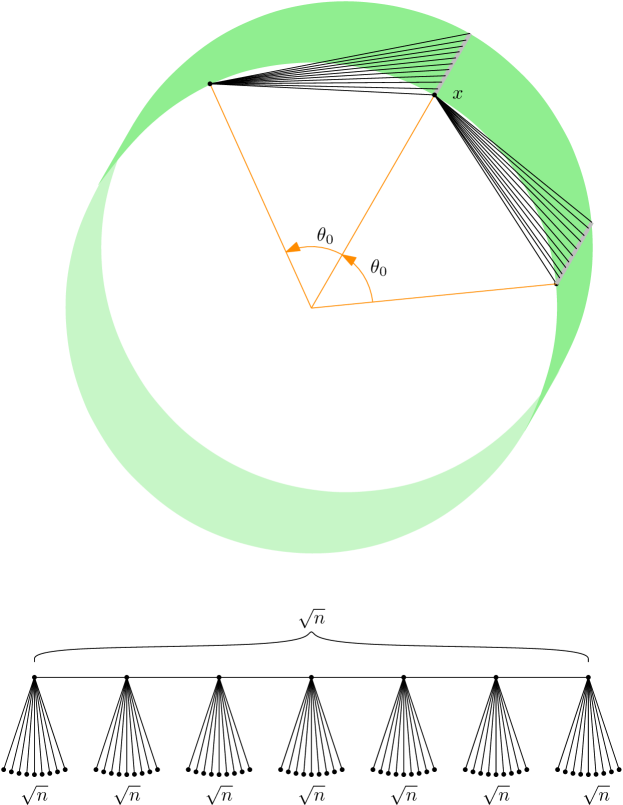
Figure 1. Modeling ${\rm FO}_{1}^{\rm local}$-limit of a $\sqrt{n}$-path of stars of order $\sqrt{n}$. Vertex $x$ is adjacent to $2^{\aleph_{0}}$ vertices on a segment and to two vertices obtained by rotation of $\pm\theta_{0}$, where $\theta_{0}$ is irrational to $\pi$.

8.2. Limit of $\rho$-non-dispersive Sequences of Trees

Let $\lambda$ be the signature of graphs, $\lambda^{\bullet}$ the signature of graphs with additional unary relation $R$, $\lambda^{+}$ the signature of graphs with additional unary relations $R$ and $P$, $\lambda^{\omega}$ the signature of graphs with countably many additional unary relations $M_{i}$ and $N_{i}$ ($i\in\mathbb{N}$). We consider two basic interpretation schemes, which we made use of already in [18]:

1. $\mathsf{I}_{Y\rightarrow F}$ is a basic interpretation scheme of $\lambda^{+}$-structures in $\lambda^{\bullet}$-structures defined as follows: for every $\lambda$-structure $\mathbf{A}$, the domain of $\mathsf{I}_{Y\rightarrow F}(\mathbf{A})$ is the same as the domain of $\mathbf{A}$, and it holds (for every $x,y\in A$):

   $$\mathsf{I}_{Y\rightarrow F}(\mathbf{A})\models x\sim y \quad\iff\quad\mathbf{A}\models(x\sim y)\wedge\neg R(x)\wedge\neg R(y)$$

   $$\mathsf{I}_{Y\rightarrow F}(\mathbf{A})\models R(x) \quad\iff\quad\mathbf{A}\models(\exists z)\ R(z)\wedge(z\sim x)$$

   $$\mathsf{I}_{Y\rightarrow F}(\mathbf{A})\models P(x) \quad\iff\quad\mathbf{A}\models R(x)$$

   In particular, if $Y$ is a $\lambda^{\bullet}$-tree, with a single vertex marked by $R$ (the root), $\mathsf{I}_{Y\rightarrow F}$ maps $Y$ into a $\lambda^{+}$-forest $\mathsf{I}_{Y\rightarrow F}(Y)$, formed by the subtrees rooted at the sons of the former root (roots marked by $R$) and a single vertex rooted principal component (the former root, marked $P$);

2. $\mathsf{I}_{F\rightarrow Y}$ is a basic interpretation scheme of $\lambda^{\bullet}$-structures in $\lambda^{+}$-structures defined as follows: for every $\lambda^{+}$-structure $\mathbf{A}$, the domain of $\mathsf{I}_{F\rightarrow Y}(\mathbf{A})$ is the same as the domain of $\mathbf{A}$, and it holds (for every $x,y\in A$):

   $$\mathsf{I}_{F\rightarrow A}(\mathbf{A})\models x\sim y \quad\iff\quad\mathbf{A}\models(x\sim y)\vee R(x)\wedge P(y)\vee R(y)\wedge P(x)$$

   $$\mathsf{I}_{F\rightarrow A}(\mathbf{A})\models R(x) \quad\iff\quad\mathbf{A}\models P(x)$$

   In particular, $\mathsf{I}_{F\rightarrow Y}$ maps a $\lambda^{+}$-forest $F$ with all connected components rooted by $R$, except exactly one rooted by $P$ into a $\lambda^{\bullet}$-tree $\mathsf{I}_{F\rightarrow Y}(F)$ by making each non principal root a son of the principal root;

Lemma 40.

Every ${\rm FO}$-convergent $\rho$-non-dispersive sequence of rooted trees $(Y_{n})_{n\in\mathbb{N}}$ has a modeling ${\rm FO}$-limit.

Proof.

Let $(Y_{n})_{n\in\mathbb{N}}$ be an ${\rm FO}$-convergent $\rho$-non-dispersive sequence of rooted trees. Then ${\mathsf{I}}_{Y\rightarrow F}(Y_{n})_{n\in\mathbb{N}}$ is an ${\rm FO}$-convergent sequence of rooted forests. According to Theorem 36, there exist $I\subseteq\mathbb{N}$, reals $\alpha_{i}$, sequences $(B_{i,n})_{n\in\mathbb{N}}$ for $i\in I\cup\{0\}$, such that:

• $\alpha_{0}\geq 0$, $\alpha_{i}>0$ (for $i\in I$), and $\sum_{i\in I\cup\{0\}}\alpha_{i}=1$;

• $Y_{n}$ is the union of the $B_{i,n}$ ($i\in I\cup\{0\}$);

• $\lim_{n\rightarrow\infty}|B_{i,n}|/|Y_{n}|=\alpha_{i}$ (for $i\in I\cup\{0\}$);

• $(B_{0,n})_{n\in\mathbb{N}}$ is an ${\rm FO}^{\rm local}$-convergent residual sequence if $\alpha_{0}>0$;

• $(B_{i,n})_{n\in\mathbb{N}}$ is an ${\rm FO}^{\rm local}$-convergent non-dispersive sequence;

• the family $\{(B_{i,n},\rho_{i,n})_{n\in\mathbb{N}}:i\in I\}$ is uniformly elementarily convergent.

In this situation we apply Theorem 37:

We denote by $\mathbf{L}_{i}$ and $\mathbf{L}_{0}$ the modeling limits, so that

• $(B_{i,n})\xrightarrow{{\rm FO}}\mathbf{L}_{i}$ (for $i\in\mathbb{N}$);

• $(B_{0,n})\xrightarrow{{\rm FO}}\mathbf{L}_{0}$ (if $\alpha_{0}>0$), and $(B_{0,n})\xrightarrow{{\rm FO}_{0}}\mathbf{L}_{0}$ (otherwise).

Then we have (by Theorem 37):

$$Y_{n}\xrightarrow{{\rm FO}}\mathsf{I}_{F\rightarrow Y}\bigl{(}\coprod_{i\in I\cup\{0\}}(\mathbf{L}_{i},\alpha_{i})\bigr{)}.$$

It is easily checked that each sequence $(B_{i,n})_{n\in\mathbb{N}}$ is $\rho$-non-dispersive (for $B_{i,n}$ rooted at its marked vertex), as a direct consequence of the fact that $(Y_{n})_{n\in\mathbb{N}}$ (rooted at marked vertex) is $\rho$-non-dispersive.

If we repeat the same process on each $\rho$-non-dispersive sequence $(B_{i,n})_{n\in\mathbb{N}}$ (for $i\in I\setminus\{0\}$), we inductively construct a countable rooted tree $S$ and, associated to each node $v$ of the tree, a residual sequence of forests $(F_{v,n})_{n\in\mathbb{N}}$ and a weight $\lambda_{v}$. If we have started with a $\rho$-non-dispersive sequence, then for every $\epsilon>0$ there is integer $d$ such that the sum of the measures of the residues attached to the nodes at height at most $d$ is at least $1-\epsilon$.

According to Lemma 39, for each residual ${\rm FO}$-convergent sequence $(F_{v,n})_{n\in\mathbb{N}}$ of forests there is a rooted tree modeling $\mathbf{L}^{0}_{v}$ that is the ${\rm FO}_{1}^{\rm local}$-limit of $({\mathsf{I}}_{F\rightarrow Y}(F_{v,n}))_{n\in\mathbb{N}}$. Hence, according to Lemmas 20, 21, and 23, there is a rooted tree modeling $\mathbf{L}_{v}$, which is the ${\rm FO}$-limit of $({\mathsf{I}}_{F\rightarrow Y}(F_{v,n}))_{n\in\mathbb{N}}$.

The grafting of the modelings $\mathbf{L}_{v}$ on the rooted tree $S$ (with weights $\lambda_{v}$) form a final modeling $\mathbf{L}$.

We prove that $\mathbf{L}$ is a relational sample space: each first-order definable subset of $L^{p}$ is a $\mathcal{L}_{\omega_{1}\omega}$-definable subsets of the countable union of all the $\mathbf{L}_{v}$ in which the roots of all the roots have been marked by distinct unary relations $M_{v}$. As the used language in countable, it follows from Lemma 7 that $\mathcal{L}_{\omega_{1}\omega}$-definable subsets are Borel measurable.

Let $d\in\mathbb{N}$, and let $Y_{n}^{(d)}$ be the subtree of $Y_{n}$ induced by vertices at distance at most $d$ from the root. As the trees $Y_{n}^{(d)}$ are obtained by an obvious interpretation, we get that $(Y_{n}^{(d)})_{n\in\mathbb{N}}$ is ${\rm FO}$-convergent. Now consider $\mathbf{L}^{(d)}$, obtained from $\mathbf{L}$ by restricting to the set $X_{d}$ of the vertices at distance at most $d$ from the root. As the set $X_{d}$ is first-order defined, it is measurable. It follows that $X_{d}$ (with induced $\sigma$-algebra) is a standard Borel space, and that $\mathbf{L}^{(d)}$ is a relational sample space. We define a probability measure on $\mathbf{L}^{(d)}$ by $\nu_{\mathbf{L}^{(d)}}=\nu_{\mathbf{L}}/\nu_{\mathbf{L}}(X_{d})$, thus defining the modeling $\mathbf{L}^{(d)}$. By applying iteratively (at depth $d$) Theorem 37 and the interpretation $\mathsf{I}_{F\rightarrow Y}$ we easily deduce that $\mathbf{L}^{(d)}$ is a modeling ${\rm FO}$-limit of $(Y_{n}^{(d)})_{n\in\mathbb{N}}$. Thus, according to Lemma 28, we deduce that $\mathbf{L}$ is a modeling ${\rm FO}^{\rm local}$-limit of the sequence $(Y_{n})_{n\in\mathbb{N}}$. By Lemma 27, we deduce that $(Y_{n})_{n\in\mathbb{N}}$ has a modeling ${\rm FO}$-limit, which is the union of $\mathbf{L}$ and a countable graph. ∎

Theorem 2.

Every ${\rm FO}$-convergent sequence of finite forests has a modeling ${\rm FO}$-limit that satisfies the Strong Finitary Mass Transport Principle.

Proof.

The theorem is an immediate consequence of Theorem 1 and Lemmas 39 and 40. ∎

9. Conclusion

Compared to the results obtained in [18] for rooted trees with bounded height, we do not have inverse theorem for tree-modeling. Our conjecture is that a tree-modeling that satisfy the Strong Finitary Mass Transport Principle and whose complete theory has the finite model property is the modeling limit of a sequence of finite trees.

We believe that our approach can be used to obtain modeling limits of further classes of graphs. In particular, we believe that the structure “residual limits grafted on a countable skeleton” might well be universal for sequences of nowhere dense graphs.

References

- [1] I. Benjamini and O. Schramm, Recurrence of distibutional limits of finite planar graphs, Electron. J. Probab. 6 (2001), no. 23, 13pp.
- [2] D. Clayton-Thomas, Spinning wheel, song by Blood, Sweat & Tears, 1969.
- [3] H. Gaifman, On local and non-local properties, Proceedings of the Herbrand Symposium, Logic Colloquium ’81, 1982.
- [4] M. Grohe, S. Kreutzer, and S. Siebertz, Deciding first-order properties of nowhere dense graphs, arXiv:1311.3899 [cs.LO], November 2013.
- [5] C. R. Karp, Languages with expressions of infinite length, vol. 33, North-Holland Pub. Co., 1964.
- [6] A. Kechris, Classical descriptive set theory, Springer-Verlag, 1995.
- [7] D. Kráľ, M. Kupec, and V. Tůma, FO limits of trees, oral presentation at Utrecht Graphs Workshop 2013, November 2013.
- [8] D. Lascar, La théorie des modèles en peu de maux, Cassini, 2009.
- [9] E.G.K. Lopez-Escobar, An interpolation theorem for infinitely long sentences, Fundamenta Mathematicae 57 (1965), 253–272.
- [10] L Lovász, Large networks and graph limits, Colloquium Publications, vol. 60, American Mathematical Society, 2012.
- [11] L. Lovász and B. Szegedy, Limits of dense graph sequences, J. Combin. Theory Ser. B 96 (2006), 933–957.
- [12] J. Nešetřil and P. Ossona de Mendez, First order properties on nowhere dense structures, The Journal of Symbolic Logic 75 (2010), no. 3, 868–887.
- [13] by same author, From sparse graphs to nowhere dense structures: Decompositions, independence, dualities and limits, European Congress of Mathematics, European Mathematical Society, 2010, pp. 135–165.
- [14] by same author, Sparse combinatorial structures: Classification and applications, Proceedings of the International Congress of Mathematicians 2010 (ICM 2010) (Hyderabad, India) (R. Bhatia and A. Pal, eds.), vol. IV, World Scientific, 2010, pp. 2502–2529.
- [15] by same author, On nowhere dense graphs, European Journal of Combinatorics 32 (2011), no. 4, 600–617.
- [16] by same author, A model theory approach to structural limits, Commentationes Mathematicæ Universitatis Carolinæ 53 (2012), no. 4, 581–603.
- [17] by same author, Sparsity (graphs, structures, and algorithms), Algorithms and Combinatorics, vol. 28, Springer, 2012, 465 pages.
- [18] by same author, A unified approach to structural limits (with application to the study of limits of graphs with bounded tree-depth), arXiv:1303.6471v2 [math.CO], October 2013.
- [19] D. Scott, Logic with denumerably long formulas and finite strings of quantifiers, The theory of models 1104 (1965), 329–341.
- [20] D. Scott and A. Tarski, The sentential calculus with infinitely long expressions, Colloquium Mathematicae, vol. 6, Institute of Mathematics Polish Academy of Sciences, 1958, pp. 165–170.
- [21] A. Tarski, Remarks on predicate logic with infinitely long expressions, Colloquium Mathematicum 16 (1958), 171–176.