KEK-TH-1691
Physics Reach of Atmospheric Neutrino Measurements at PINGU

Abstract

The sensitivity of a huge underground water/ice Cherenkov detector, such as PINGU in IceCube, to the neutrino mass hierarchy, the atmospheric mixing angle and its octant, is studied in detail. Based on the event rate decomposition in the propagation basis, we illustrate the smearing effects from the neutrino scattering, the visible energy and zenith angle reconstruction procedures, the energy and angular resolutions, and the muon mis-identification rate, as well as the impacts of systematic errors in the detector resolutions, the muon mis-identification rate, and the overall normalization. The sensitivity, especially the mass hierarchy sensitivity, can be enhanced by splitting the muon-like events into two channels, according to the event inelasticity. We also show that including the cascade events can improve and stabilize the sensitivity of the measurements.

1 Introduction

The reactor mixing angle, $\theta_{13}$, has been measured in the last two years. Following T2K [1], MINOS [2] and Double Chooz [3] indicated that $\theta_{13}$ is nonzero, reaching $3.5\,\sigma$ in a combined analysis [4]. The conclusive results of a large reactor mixing angle come from Daya Bay [5] and RENO [6] with significance up to $7.7\,\sigma$ [7]. These progresses open up the opportunity [8, 9, 10] to measure the three remaining unknown parameters in neutrino oscillation, namely the neutrino mass hierarchy, the octant of the atmospheric mixing angle, and the CP phase.

The neutrino mass hierarchy can be measured [11] by medium-baseline reactor experiments, such as JUNO [12] and RENO-50 [13], atmospheric neutrino experiments, such as PINGU (Precision Icecube Next Generation Upgrade) [14], Hyper-K [15, 16], INO [17, 18], or a liquid argon detector [19, 20, 21, 22], and accelerator based long-baseline (LBL) experiments such as NO$\nu$A [23, 24] or LBNE [25]. The reactor based experiments focus on the neutrino mass hierarchy while atmospheric neutrino experiments can measure both the neutrino mass hierarchy and the atmospheric mixing angle. In addition to the neutrino mass hierarchy, accelerator experiments [26] can measure the CP phase [27], including NO$\nu$A [23, 24], T2K [28], T2HK [15, 16, 29], and LBNE [25]. By splitting the running time between neutrino and antineutrino, it is also possible for accelerator experiments to achieve stable sensitivity to the octant of the atmospheric mixing angle [30, 27, 31].

For atmospheric neutrino experiments, different ways have been developed to analyse the oscillation pattern, including oscillogram [32, 33, 34, 35, 36, 37, 37, 38] and event-rate decomposition [39]. The former emphasizes the overall structure, especially for the resonance behavior, while the later is designed for separating the contributions of the three unknown parameters hidden in the overall pattern and hence is very powerful to unveil the trend in $\chi^{2}$ minimization. In principle, the oscillogram can also be applied to the coefficients of analytically decomposed terms, making their overall pattern explicit. Here, we apply the algorithm developed in [39] on the physics reach of the PINGU experiment. The sensitivity of PINGU has been explored extensively in the literature [40, 41, 42, 43, 44, 45, 46, 39] for the neutrino mass hierarchy, and in [40, 47, 48, 39] for the octant of the atmospheric mixing angle. There are some brief discussions on the CP phase [40, 49, 39].

In this paper, we study in detail the physics reach of atmospheric neutrino oscillation measurements at the PINGU detector, concerning the sensitivity to the neutrino mass hierarchy, the precision on the atmospheric mixing angle and the sensitivity to its octant. This paper is organized as follows. In Sec. 2, the formalism of event-rate decomposition in the propagation basis is summarized. In Sec. 3 we present the basic features of neutrino scattering, especially the inelasticity distribution which can be used to enhance the sensitivity to the neutrino mass hierarchy, and reconstruction procedures of the visible energy and zenith angle, leaving discussions on the detector resolutions to Sec. 4. The impacts of all these smearing effects are studied step by step in Sec. 5. Finally in Sec. 6, we examine possible impacts of a few systematic errors, including those in energy and angular resolutions, muon mis-identification rate, and overall normalization, and the conclusion can be found in Sec. 7.

2 Event-Rate Decomposition in the Propagation Basis

With the reactor mixing angle being measured, there are three remaining unknowns in the three-neutrino oscillation, namely the neutrino mass hierarchy, the octant of the atmospheric mixing angle, $\theta_{\rm a}\equiv\theta_{23}$, and the CP phase, $\delta$. Their contributions to neutrino oscillation can be analytically decomposed in the propagation basis [50, 51, 52]. This formalism can apply generally and is extremely useful for the study of atmospheric neutrino oscillation where the matter potential has a complicated structure [53].

For completeness, we review the key results of the event-rate decomposition [39] in the propagation basis. By noting that the atmospheric mixing angle $\theta_{\rm a}$ and the CP phase $\delta$ dependences of the oscillation amplitudes do not suffer from the matter effects in the propagation basis, one can express analytically their dependences of all the oscillation probabilities, and hence the expected event rates in any neutrino experiments/observations. The following decompositions for the muon-like ($\alpha=\mu$) and the cascade ($\alpha=e$) event rates were proposed for phenomenological studies,

$$\frac{\partial^{2}N_{\alpha}(E_{\nu},\cos\theta^{\nu}_{\rm z})}{\partial E_{\nu}\partial\cos\theta^{\nu}_{\rm z}}=N^{(0)}_{\alpha}+N^{(1)}_{\alpha}x_{\rm a}+N^{(2)}_{\alpha}\cos\delta^{\prime}+N^{(3)}_{\alpha}\sin\delta^{\prime}+N^{(4)}_{\alpha}x_{\rm a}\cos\delta^{\prime}+N^{(5)}_{\alpha}x^{2}_{\rm a}+N^{(6)}_{\alpha}\cos^{2}\delta^{\prime}+\mathcal{O}(x^{4}_{\rm a})\,,$$ (2.1)

where,

$$x_{\rm a}\equiv\cos 2\theta_{\rm a}=\cos^{2}\theta_{\rm a}-\sin^{2}\theta_{\rm a}\,,$$ (2.2)

parametrizes the dependence of the oscillation probabilities on the atmospheric mixing angle $\theta_{\rm a}$, taking a positive value for the lower octant (LO), $\sin^{2}\theta_{\rm a}<0.5$, and a negative value for the higher octant (HO), $\sin^{2}\theta_{\rm a}>0.5$. The CP phase $\delta$ dependence appear only through the combinations,

$$\cos\delta^{\prime}\equiv\sin 2\theta_{\rm a}\cos\delta=\sqrt{1-x^{2}_{\rm a}}\cos\delta\,,\qquad\sin\delta^{\prime}\equiv\sin 2\theta_{\rm a}\sin\delta=\sqrt{1-x^{2}_{\rm a}}\sin\delta\,,$$ (2.3)

since $\cos\delta$ or $\sin\delta$ are always modulated by a common prefactor $\sin 2\theta_{\rm a}$. The accuracy of measuring the CP phase decreases when the atmospheric mixing angle deviates from its maximal value. Note that the expansion is up to order $x^{2}_{\rm a}$ as the terms of order $x^{4}_{\rm a}$ are found to be negligibly small [39] in the $3\,\sigma$ allowed range,

$$x^{2}_{\rm a}=1-\sin^{2}2\theta_{\rm a}<0.052\,.$$ (2.4)

For atmospheric neutrino oscillation, the coefficients $N^{(k)}_{\mu}$ and $N^{(k)}_{\rm e}$ ($k=0,\cdots,6$) give the neutrino energy, $E_{\nu}$, and the zenith angle, $\cos\theta^{\nu}_{\rm z}$, dependences of the muon-like and cascade event rates, respectively, which dependent on the solar mixing angle, $\theta_{\rm s}\equiv\theta_{12}$, the reactor mixing angle, $\theta_{\rm r}\equiv\theta_{13}$, and the two mass squared differences, $\delta m^{2}_{\rm a}\equiv m^{2}_{3}-m^{2}_{1}$ and $\delta m^{2}_{\rm s}\equiv m^{2}_{2}-m^{2}_{1}$, and hence on the neutrino mass hierarchy, normal ($\delta m^{2}_{\rm a}>0$) or inverted ($\delta m^{2}_{\rm a}<0$). These coefficients are obtained by the convolution integrals,

$$N^{(k)}_{\alpha}(E_{\nu},\cos\theta^{\nu}_{\rm z}) = \sum_{\beta={\rm e},\mu}\left[\phi_{\nu_{\beta}}(E_{\nu},\cos\theta^{\nu}_{\rm z})\times P^{(k)}_{\beta\alpha}(E_{\nu},\cos\theta^{\nu}_{\rm z})\times\sigma_{\nu_{\alpha}}(E_{\nu})\right.$$ (2.5)

$$\hskip 19.91692pt\left.+\phi_{\bar{\nu}_{\beta}}(E_{\nu},\cos\theta^{\nu}_{\rm z})\times\overline{P}^{(k)}_{\beta\alpha}(E_{\nu},\cos\theta^{\nu}_{\rm z})\times\sigma_{\bar{\nu}_{\alpha}}(E_{\nu})\right]\times\rho V_{\rm eff}(E_{\nu})\,,$$

where $\phi_{\nu_{\beta}}$ and $\phi_{\bar{\nu}_{\beta}}$ are the $\nu_{\beta}$ and $\bar{\nu}_{\beta}$ fluxes at the South Pole [54], $P^{(k)}_{\beta\alpha}$ and $\overline{P}^{(k)}_{\beta\alpha}$ are, respectively, the relevant coefficients of the $\nu_{\beta}\rightarrow\nu_{\alpha}$ and $\bar{\nu}_{\beta}\rightarrow\bar{\nu}_{\alpha}$ oscillation probabilities [39], $\sigma_{\nu_{\alpha}}$ and $\sigma_{\bar{\nu}_{\alpha}}$ denote the $\nu_{\alpha}$ and $\bar{\nu}_{\alpha}$ cross sections via the charged current (CC) scattering off the water target obtained with NEUGEN [55], and $\rho V_{\rm eff}$ is the effective fiducial volume of the detector. Although the atmospheric neutrino flux for $\nu_{\tau}$ or $\bar{\nu}_{\tau}$ is negligibly small [54], we can account for the $\nu_{\tau}$ and $\bar{\nu}_{\tau}$ scattering contributions, by using the same formula (2.5) for $\alpha=\tau$, even though the effective fiducial volume for $\tau$-CC and neutral current (NC) events may be much smaller than those of $\mu$-CC and e-CC events [56].

The coefficients of those terms independent of CP phase $\delta$, namely $N^{(0)}_{\alpha}$, $N^{(1)}_{\alpha}$, and $N^{(5)}_{\mu}$, are at least one order of magnitude larger than those of $\delta$-dependent terms: $N^{(2)}_{\alpha}$, $N^{(3)}_{\alpha}$, and $N^{(4)}_{\mu}$ are of the order $\mathcal{O}(\delta m^{2}_{\rm s}/\delta m^{2}_{\rm a})$, while $N^{(6)}_{\mu}$ is suppressed by $(\delta m^{2}_{\rm s}/\delta m^{2}_{\rm a})^{2}$ as compared to the overall rates of $N^{(0)}_{\alpha}$. Note that the cascade event rates have no nonlinear dependence on $x_{\rm a}$ and $\cos\delta^{\prime}$, $N^{(4)}_{\rm e}=N^{(5)}_{\rm e}=N^{(6)}_{\rm e}=0$. The smallness or absense of the coefficients $N^{(k)}_{\alpha}$ for $k=2,3,4,6$ in (2.1) are consequences of the smallness or absense of the corresponding oscillation probabilities $P^{(k)}_{\beta\alpha}$ and $\overline{P}^{(k)}_{\beta\alpha}$ for $k=2,3,4,6$ [39]. These features tell that the neutrino mass hierarchy and the atmospheric mixing angle can have sizable effects and hence be measured at PINGU, but it is more challenging to measure the CP phase. In this paper, we concentrate on the sensitivity of PINGU to the neutrino mass hierarchy, its expected accuracy of measuring the atmospheric mixing angle $\theta_{\rm a}$, parametrized as $x_{\rm a}$, and sensitivity to its octant ($x_{\rm a}<0\mbox{ or }x_{\rm a}>0$).

In Fig. 1, we show the relevant coefficients of the $\delta$-independent terms in (2.1), $N^{(0)}_{\mu}$ (red curves) and $N^{(1)}_{\mu}$ (blue curves) in the left, $N^{(0)}_{\rm e}$ (red curves) and $N^{(1)}_{\rm e}$ (blue curves) in the center, and $N^{(5)}_{\mu}$ in the right panels, in the region of $1\,\mbox{GeV}<E_{\nu}<20\,\mbox{GeV}$ for give zenith angles $\cos\theta^{\nu}_{\rm z}=-1,-0.9,-0.8,-0.6,-0.4$ of the neutrino momentum direction. The nominal number of events per GeV for one-year run of PINGU is shown along the vertical axis. Note that, the plots in Fig. 1 have been updated from those of [39] by accounting for the fiducial volume for 40-string configuration, which is obtained from the 20-string configuration [45] by rescaling the neutrino energy, $V^{(40)}_{\rm eff}(E_{\nu})=V^{(20)}_{\rm eff}(2\times E_{\nu})$. Since the full-detector simulation of the PINGU detector is not available yet, and the fact that the tau neutrino contribution is negligible while the difference between the effective fiducial volumes for muon and electron neutrino is not so large according to a preliminary simulation [56], we just assume that the effective fiducial volume is the same for different flavors.

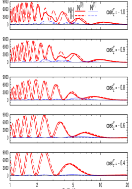
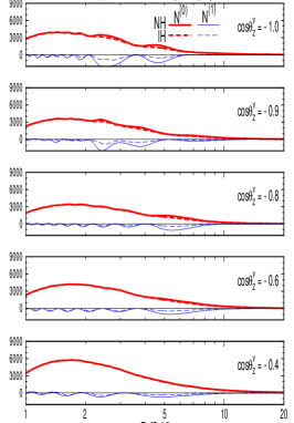
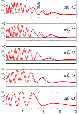
Fig. 1: The coefficients of $\delta$-independent terms in the propagation-basis decomposition of the muon-like and cascade event rates, with normal hierarchy (NH) [solid curves] and inverted hierarchy (IH) [dashed curves]. The number of events, $N^{(0)}_{\alpha}+N^{(1)}_{\alpha}x_{\rm a}+N^{(5)}_{\alpha}x^{2}_{\rm a}$, corresponds to nominal expectation of 40-string PINGU in 1 year.

First, for the overall event rates of $N^{(0)}_{\alpha}$, shown by the red curves in the left ($\alpha=\mu$) and the center ($\alpha={\rm e}$) panels, the cascade event rates have a much smoother energy and angular dependence than the muon-like event rates. In addition, the cascade event rates are consistently larger for the normal hierarchy (NH), shown by red-solid curves, than for the inverted hierarchy (IH), shown by the red-dashed curves in the center panel, while the muon-like event rates have strong oscillatory pattern where the region of NH v.s. IH dominance alter frequently with neutrino energy, $E_{\nu}$, and somewhat also with the zenith angle, $\cos\theta^{\nu}_{\rm z}$. These features suggest that the cascade events may be more stable against the energy-angular smearing effects than the muon-like events, as will be discussed in Sec. 3 and Sec. 4.

Another notable feature in Fig. 1 is that, $N^{(1)}_{\mu}$ is always positive while $N^{(1)}_{\rm e}$ is always negative, for the coefficients of the $x_{\rm a}$ term. More closely examining the curves, we note that the difference between NH and IH in the event rates, $N^{(0)}_{\alpha}+N^{(1)}_{\alpha}\,x_{\rm a}$, tends to increase for the negative $x_{\rm a}$, both for the muon-like and cascade events. Therefore, we expect the neutrino mass hierarchy discrimination by atmospheric neutrino oscillation to be easier for the higher octant, $x_{\rm a}<0(\sin^{2}\theta_{\rm a}>0.5)$, than for the lower octant, $x_{\rm a}>0(\sin^{2}\theta_{\rm a}<0.5)$.

The coefficient $N^{(5)}_{\mu}$ of the quadratic term $x^{2}_{\rm a}$ is shown in the right panel. Note that this quadratic term only appears in the muon-like events. It can dominate over $N^{(0)}_{\mu}$ and $N^{(1)}_{\mu}$ around the oscillation minima in the energy range $5\,\mbox{GeV}\lesssim E_{\nu}\lesssim 10\,\mbox{GeV}$ where both $N^{(0)}_{\mu}$ and $N^{(1)}_{\mu}$ are tiny but $N^{(5)}_{\mu}$ is larger by an order of magnitude, because the oscillation phases (the location of this minima) are different between $N^{(0)}_{\mu}$ and $N^{(5)}_{\mu}$ [39]. In the whole range, $N^{(5)}_{\mu}$ is always positive. More importantly, $N^{(5)}_{\mu}$ has opposite phase w.r.t. $N^{(0)}_{\mu}$. For example, $N^{(5)}_{\mu}$ peaks around $E_{\nu}=5\,\mbox{GeV}$ and $\cos\theta^{\nu}_{\rm z}=-1$, with larger event rate for IH, where it is a minimum for $N^{(0)}_{\mu}$ with larger event rate for NH. The hierarchy sensitivity in $N^{(5)}_{\mu}$ always cancels with the one in $N^{(0)}_{\mu}$. In other words, the quadratic term reduces the hierarchy sensitivity in the muon-like event rates. Summing up, the mass hierarchy dependence of the event rate, $N^{(0)}_{\mu}+N^{(1)}_{\mu}\,x_{\rm a}+N^{(5)}_{\mu}\,x^{2}_{\rm a}$, tends to decrease as $x^{2}_{\rm a}$ increases or $x_{\rm a}$ increases. Consequently, it decreases when $x_{\rm a}$ is positive and $x^{2}_{\rm a}$ increases. If $x_{\rm a}$ is negative, the trend depends on which one of the effects from the linear term and quadratic term of $x_{\rm a}$ dominates. Since $N^{(5)}_{\mu}$ can dominate over $N^{(0)}_{\mu}$ and $N^{(1)}_{\mu}$ when $x_{\rm a}\approx-0.2$, the effect of the quadratic term dominates. Hence, the sensitivity decreases when $x_{\rm a}$ is negative and decreases.

Due to the Earth matter potential, neutrinos travelling through the mantle can experience MSW resonance [57, 58, 59, 60] while those travelling through the core can experience an extra parametric resonance [61, 62, 63, 64] which is also known as oscillation-length resonance [65, 66, 67, 33]. This only happens for the case of neutrino with NH or antineutrino with IH. If neutrino events can be distinguished from antineutrino events, the sensitivity to the neutrino mass hierarchy by observing the atmospheric neutrino oscillation pattern can improve significantly. The study in [39], as summarized above in Fig. 1, assumes that PINGU cannot discriminate between neutrino and antineutrino events, and hence all the hierarchy dependence of the observed event numbers are due to the difference in the neutrino and antineutrino fluxes [54], and in the CC cross sections [55]. Luckily, both the fluxes and the cross sections are larger for neutrino than antineutrino, resulting in the significant hierarchy dependence for muon-like and cascade events. In the following Sec. 3, we will show how one can use the inelasticity distribution of muon CC events to discriminate between $\nu_{\mu}$ and $\bar{\nu}_{\mu}$ events, which can further improve the hierarchy sensitivity of the experiment.

3 Neutrino Scattering and Reconstruction Procedures

Experimentally, neutrino momentum cannot be directly measured. Neutrinos interact with the target, generating various final-state particles, some of which can leave traces in the detector. These traces are measured to reconstruct the energy and momentum of the final-state particles and then the incident neutrino momentum is estimated via the energy-momentum conservation. Because the detector responses to the muon, electron, and hadron are different, reconstruction of the incident neutrino momentum is not only difficult but also depends on the reaction. The visible neutrino energy, $E_{\rm vis}$, and its visible momentum direction, $\cos\theta^{\rm vis}_{\rm z}$, distribute around their true values, $E_{\nu}$ and $\cos\theta^{\nu}_{\rm z}$. The resulting observable distributions significantly smear the oscillation patterns in neutrino event rates, as shown in Fig. 1, and reduce the sensitivities discussed in [39]. On the brighter side, the topology of the final-state particles in the charged current (CC) scattering of neutrino is significantly different from that of antineutrino. This feature can be used to distinguish neutrino from antineutrino statistically for CC events and enhance the sensitivity to the neutrino mass hierarchy.

3.1 Neutrino Scattering and Inelasticity Distribution

Since the information of neutrino oscillation is kept only in the CC scattering, we will focus on the following processes,

$$\nu_{\ell}+N \rightarrow \ell+X\,,$$ (3.1a)

$$\bar{\nu}_{\ell}+N \rightarrow \bar{\ell}+X\,,$$ (3.1b)

where $N$ is the target nucleon and $X$ represents the final-state hadrons, for $\ell=e\mbox{ or }\mu$. In terms of the Bjorken scaling variables, the differential cross section per nucleon can be expressed in the parton model as [68, 69],

$$\frac{\partial^{2}\sigma_{\nu}}{\partial x\partial y} = \frac{2G^{2}_{F}ME_{\nu}}{\pi}\left[xq(x,Q^{2})+x\bar{q}(x,Q^{2})(1-y)^{2}\right]\,,$$ (3.2a)

$$\frac{\partial^{2}\sigma_{\bar{\nu}}}{\partial x\partial y} = \frac{2G^{2}_{F}ME_{\bar{\nu}}}{\pi}\left[x\bar{q}(x,Q^{2})+xq(x,Q^{2})(1-y)^{2}\right]\,,$$ (3.2b)

with $x\equiv Q^{2}/2M(E_{\nu}-E_{\ell})$ and inelasticity $y\equiv(E_{\nu}-E_{\ell})/E_{\nu}$ for neutrino and similarly for antineutrino. Here $q(x,Q^{2})$ and $\bar{q}(x,Q^{2})$ are the quark and antiquark distributions in the nucleon measured at the momentum transfer scale of $Q^{2}\equiv 2E_{\nu}E_{\ell}(1-\cos\theta_{\ell})$. Because the quark distribution $q(x,Q^{2})$ is much larger than the antiquark distribution $\bar{q}(x,Q^{2})$ in nuclei, the $\nu$–CC events are expected to have relatively flat distribution of inelasticity, whereas the $\bar{\nu}$–CC events have strong suppression at large inelasticity due to the $(1-y)^{2}$ factor multiplying the quark distribution $q(x,Q^{2})$ in (3.2b). After integrating over $y$, the total cross section of antineutrino is roughly one third of that of neutrino for an isoscalar nucleon. We therefore expect that at small inelasticity, $1-y\approx 1$, the antineutrino cross section $\sigma_{\bar{\nu}}$ is as large as the neutrino cross section $\sigma_{\nu}$, but at large inelasticity, $1-y\approx 0$, $\sigma_{\bar{\nu}}$ is much smaller than $\sigma_{\nu}$. We can enhance the purity of the $\nu$–CC events by selecting those events with $1-y\approx 0$, where those events at $1-y\approx 1$ is a mixture of $\nu$– and $\bar{\nu}$–CC events, whose ratio may reflect that of the original fluxes.

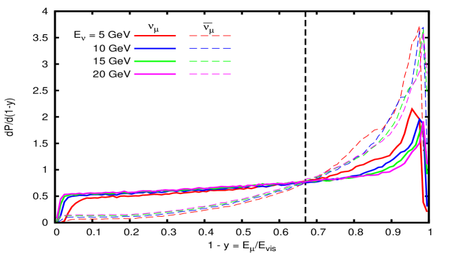
Fig. 2: Inelasticity distribution of neutrino (solid curves) and antineutrino (dashed curves) CC scattering.

We use GENIE [70] to obtain the inelasticity distribution as shown in Fig. 2, for $\nu_{\mu}$– and $\bar{\nu}_{\mu}$–CC events off water target. The normalized cross sections are shown by solid curves for $\nu_{\mu}$ and by dashed curves for $\bar{\nu}_{\mu}$, for neutrino energies of 5, 10, 15, and $20\,\mbox{GeV}$. It is amusing to note that the normalized distributions cross at $1-y\approx 0.67$, which is stable in the energy range of $5\,\mbox{GeV}\lesssim E_{\nu}\lesssim 20\,\mbox{GeV}$. Note that the inelasticity shown in Fig. 2 is defined in terms of the visible energy $E_{\rm vis}$, instead of $E_{\nu}$,

$$1-y\equiv\frac{E_{\ell}}{E_{\rm vis}}\,,$$ (3.3)

where $E_{\rm vis}$ will be defined in the next section. The smearing effects detailed in Sec. 3.2 and Sec. 4 have already been accounted for in order to make a realistic illustration.

Experimentally, there are several ways of distinguishing neutrino from antineutrino. The charge of the lepton can be measured by applying magnetic field to the detector, such as ICAL [18] and a liquid argon detector [20], to tell if it is produced in CC scattering by neutrino or antineutrino. For those detectors implementing magnetic field is not possible, such as Super-K [15, 16], distinct signal, such as the delayed signal in single-ring electron events, or characteristic distribution, such as the inelasticity dependence of multi-ring electron events, can be used. The latter method can also apply to PINGU [71, 42] for muon-CC events, which will be studied in the following sections.

3.2 Reconstruction Procedures

Neutrino scattering can smear the oscillation pattern since it is impossible to directly measure the neutrino momentum. The information can only be partially retrieved by reconstructing from the final-state particles that are observable. For CC events, in principle it is possible to reconstruct the incident neutrino momentum, whereas a sizable fraction of the momentum is lost in the neutral current (NC) as well $\tau$-CC events. This effect is especially severe for atmospheric neutrino experiments where the direction of the incident neutrino is unknown. In this section, we discuss the energy and zenith angle reconstruction procedures, leaving the detector resolutions to be studied in Sec. 4. The reconstruction procedures assumed here are intuitive and need to be enriched by full-detector simulation which is not available yet.

3.2.1 Energy Reconstruction

PINGU measures the Cherenkov light from the final-state particles by recording their energy and arriving time. These information can be used to reconstruct the energy and momentum of the final-state particles [72].

Depending on the particle species, the Cherenkov light yield is different. For charged lepton, muon or electron, its energy can be estimated from the Cherenkov light radiation, while the yield is significantly lower for other particle that can induce hadronic cascades, which consist of electromagnetic showers from $\pi^{0}$’s and radiations from charged pions and nucleon excitations. In the following study, we assign the equivalent visible energy of a hadronic cascade to be 80% of that of an electromagnetic shower [73, 74, 75]. Then, the cascade Cherenkov light energy can be expressed as,

$$E_{\rm cas}\equiv 0.8\times(E_{\nu}-E_{\nu^{\prime}}-E_{\ell})+E_{\rm e}\,,$$ (3.4)

where $E_{\nu}$ and $E_{\nu^{\prime}}$ are the energies of the incident and the final-state neutrinos, respectively. For $\mu$–CC and e-CC, $E_{\nu^{\prime}}=0$ and it can be large for NC and $\tau$-CC events. For $\mu$–CC events, $E_{\ell}=E_{\mu}$ and $E_{\rm e}=0$, while for e–CC events, $E_{\ell}=E_{\rm e}$.

There are two typical topologies on PINGU. Muon with large enough energy, $E_{\mu}>1\,\mbox{GeV}$, leaves a clear track due to its long lifetime while the cascade produced by other particles has a spherical structure. Because of this difference, the energies of muon and cascade can be reconstructed independently. This distinguishability makes estimating the muon inelasticity possible, as defined in (3.3). On the other hand, the electron shower cannot be distinguished from cascade, hence, its energy cannot be measured separately. For muon with small energy, $E_{\mu}<1\,\mbox{GeV}$, the track may not be long and clear enough to be identified, and it is counted as cascade events. In addition, 10% of the energetic muons, $E_{\mu}>1\,\mbox{GeV}$, are assumed to be mis-identified as cascade events [43]. For $\tau$, it decays very quickly into muon, electron, or hadrons. For all these cases, the visible energy can then be estimated as,

$$E_{\rm vis}\equiv E_{\mu}+\frac{E_{\rm cas}}{0.8}=\begin{cases}E_{\nu}&\mu-CC\,(E_{\mu}>1\,\mbox{GeV with 90\% }\mu\mbox{-ID})\,,\\ E_{\nu}+0.25E_{\ell^{\prime}}&\begin{cases}e-CC\,,\\[-2.84526pt] \mu-CC\,(E_{\mu}<1\,\mbox{GeV},E_{\mu}>1\,\mbox{GeV with 10\% }\mu\mbox{-misID})\,,\end{cases}\\[8.53581pt] E_{\nu}-E_{\nu^{\prime}}&\begin{cases}\tau-CC\mbox{ with }\tau\rightarrow\mu\,(E_{\mu}>1\,\mbox{GeV with 90\% }\mu\mbox{-ID})\,,\\[-2.84526pt] \tau-CC\mbox{ with }\tau\rightarrow\mbox{hadrons}\,,\\[-2.84526pt] NC\,,\end{cases}\\[2.84526pt] E_{\nu}-E_{\nu^{\prime}}+0.25E_{\ell^{\prime}}&\tau-CC\begin{cases}\tau\rightarrow e\,,\\[-2.84526pt] \tau\rightarrow\mu\,(E_{\mu}<1\,\mbox{GeV},E_{\mu}>1\,\mbox{GeV with 10\% }\mu\mbox{-misID})\,,\end{cases}\end{cases}$$ (3.5)

where $\ell^{\prime}$ denotes the electron or the mis-identified muon. In this definition, $E_{\rm vis}$ is the visible energy after rescaling the cascade energy $E_{\rm cas}$ and adding it to the muon energy $E_{\mu}$, so that for muon-like events $E_{\rm vis}$ is exactly the neutrino energy.

For e–CC events, all the final-state energies are recorded as shower energies, and hence the electron energy $E_{\rm e}$ is 25% overestimated. For $\mu$–CC events, if the muon is mis-identified as a shower, or if the muon energy $E_{\mu}$ is too low for the track reconstruction, its energy is again overestimated by 25%. The visible energy $E_{\rm vis}$ is larger than the neutrino energy $E_{\nu}$, with the difference depending on $E_{\ell^{\prime}}$ (the energy of final state electron or that of final state muon when it is mis-identified as electron), and hence contributes to the smearing effect during energy reconstruction. The typical size of the final-state lepton energy ($E_{\ell^{\prime}}$) distribution, divided by a factor of $4$, is therefore the characteristic energy resolution from energy reconstruction. Since the inelasticity distribution is quite stable as shown in Fig. 2, this characteristic energy resolution is proportional to $E_{\nu}$, independent of the neutrino energy. On average, the lepton takes away about 60% of neutrino and 80% of antineutrino energies. The smearing effect in energy reconstruction can hence be as large as $\sigma_{\rm E}\approx 0.15\times(E_{\nu}/\mbox{GeV})$ for neutrino and $\sigma_{\rm E}\approx 0.2\times(E_{\nu}/\mbox{GeV})$ for antineutrino. This explains the linear dependence of the energy resolution on the neutrino energy, $\sigma_{\rm E}\approx 0.25\times(E_{\nu}/\mbox{GeV})$, as found in [45]. The discrepancy may be due to the energy resolution originating from statistical fluctuation, $\sigma_{\rm E}\approx 0.2\times\sqrt{E_{\nu}/\mbox{GeV}}$, as will be discussed in Sec. 4.1. It is worth noting here that our very naive treatment of the energy reconstruction error tends to reproduce the simulation results [45] when combined with the expected statistical error of the measurement. The above estimation applies only to e-CC events. For NC and $\tau$-CC events with $\tau$ decaying into hadrons, the visible energy $E_{\rm vis}$ is much smaller than the neutrino energy $E_{\nu}$ due to the energy $E_{\nu^{\prime}}$ of the final-state neutrinos. Therefore, the smearing effect due to energy reconstruction is proportional to the distribution of the final-state neutrino energy $E_{\nu^{\prime}}$ which is also expected to be proportional to the neutrino energy. For the fourth case in (3.5), $\tau$–CC with tau decaying into an electron or a mis-identified muon, the smearing effect comes from both the final-state neutrino and lepton.

3.2.2 Zenith Angle Reconstruction

Depending on the path, which is a function of the zenith angle, atmospheric neutrino experiences different matter potential and baseline length. It is necessary to recover the zenith angle of the incident neutrino in order to measure the neutrino oscillation pattern. This can be achieved by reconstructing the momentum of the incident neutrino.

Since muon has a long track in the PINGU detector, its direction can be determined with a much higher precision than the cascade. If there is a muon in the final state, such as the $\mu$-CC channel and the $\tau$-CC channel with $\tau$ decaying into an energetic muon, $E_{\mu}>1\,\mbox{GeV}$, the reconstructed direction is mainly determined by the momentum of this muon. The same scenario also applies to the case with an energetic electron which can produce a forward radiation whose direction dominates in the cascade radiation. If the energy carried away by lepton is not large enough, the Cherenkov light from lepton will be overwhelmed by the hadronic radiation. Then the total visible momentum can only be estimated from the total visible momentum in the final state. These two topologies can be expressed as,

$$\vec{P}_{\rm vis}=\begin{cases}\vec{P}_{\ell}&\hskip 8.53581ptCC\,(E_{\ell}>1\,\mbox{GeV})\,,\\[2.84526pt] \vec{P}_{\nu}-\vec{P}_{\nu^{\prime}}&\begin{cases}CC\,(E_{\ell}<1\,\mbox{GeV})\,,\\[-2.84526pt] NC\,,\end{cases}\end{cases}$$ (3.6)

where $\ell$ stands for muon or electron, $\vec{P}_{\nu^{\prime}}$ denotes the vector sum of all the final-state neutrinos in NC and $\tau$-CC events, whereas $\vec{P}_{\nu^{\prime}}=0$ for muon-like and cascade CC events. In both cases, the momentum of the incident neutrino cannot be exactly reconstructed. For CC with $E_{\ell}>1\,\mbox{GeV}$, in principle, the direction of the hadronic cascade can also be used as supplementary information to help estimating the neutrino direction. But it has much worse angular resolution and we do not attempt to reconstruct the hadronic momentum vector for events with $E_{\ell}>1\,\mbox{GeV}$.

Fig. 3: Kinematics of neutrino scattering.

For convenience, the scattering process has been illustracted in Fig. 3, where $\theta^{\nu}_{\rm z}$ and $\theta^{\rm vis}_{\rm z}$ are the zenith angles of the incident neutrino momentum $\vec{P}_{\nu}$ and the visible momentum $\vec{P}_{\rm vis}$, respectively, parametrized as,

$$-\vec{P}_{\nu}\equiv\left|\vec{P}_{\nu}\right|\left\lgroup\begin{matrix}\sin\theta^{\nu}_{\rm z}\\ 0\\ \cos\theta^{\nu}_{\rm z}\end{matrix}\right\rgroup\,,\qquad-\vec{P}_{\rm vis}\equiv\left|\vec{P}_{\rm vis}\right|\left\lgroup\begin{matrix}\sin\theta^{\rm vis}_{\rm z}\cos\phi_{\rm vis}\\ \sin\theta^{\rm vis}_{\rm z}\sin\phi_{\rm vis}\\ \cos\theta^{\rm vis}_{\rm z}\end{matrix}\right\rgroup\,.$$ (3.7)

The opening angle between $\vec{P}_{\nu}$ and $\vec{P}_{\rm vis}$ is denoted as $\delta\theta$ while $\phi$ is the azimuthal angle of $\vec{P}_{\rm vis}$ with respect to $\vec{P}_{\nu}$ in the neutrino frame, where $\vec{P}_{\nu}$ gives the polar axis and the azimuthal angle is measured from the plane which contains the zenith direction vector $\vec{n}_{\rm z}$ at the South Pole, as shown in Fig. 3. With a given zenith angle $\theta^{\nu}_{\rm z}$ of the incident neutrino, the visible zenith angle $\theta^{\rm vis}_{\rm z}$ is a function of $\delta\theta$ and $\phi$,

$$\cos\theta^{\rm vis}_{\rm z}=\cos\theta^{\nu}_{\rm z}\cos\delta\theta-\sin\theta^{\nu}_{\rm z}\sin\delta\theta\cos\phi\,.$$ (3.8)

From this, we can observe that the visible zenith angle takes a value in the range of,

$$\min(0,\theta^{\nu}_{\rm z}-\delta\theta)\leq\theta^{\rm vis}_{\rm z}\leq\max(\pi,\theta^{\nu}_{\rm z}-\delta\theta)\,,$$ (3.9)

which is always within the defined range $[0,\pi]$ of the zenith angle. At very high energies, the opening angle $\delta\theta$ is tiny, and the approximation $\theta^{\rm vis}_{\rm z}\approx\theta^{\nu}_{\rm z}$ holds. At energies below $10\,\mbox{GeV}$, the opening angle can be significant, and the projection from $\theta^{\nu}_{\rm z}$ to $\theta^{\rm vis}_{\rm z}$ needs to be done carefully as follows.

The distribution of $\vec{P}_{\rm vis}$ is solely determined by the neutrino interactions. In the neutrino frame, the event distribution after scattering depends on the polar angle $\delta\theta$, but not on the azimuthal angle $\phi$ or the neutrino zenith angle $\theta^{\nu}_{\rm z}$,

$$\left.\frac{\partial^{3}N}{\partial E_{\rm vis}\partial\delta\theta\partial\phi}\right|_{E_{\nu}}\equiv\frac{1}{2\pi}\mathbb{T}(E_{\nu}|E_{\rm vis},\delta\theta)\,,$$ (3.10)

where $N$ represents the neutrino event number and the transfer table $\mathbb{T}$ describes the distribution of $\vec{P}_{\rm vis}$ for a given neutrino energy $E_{\nu}$. In the current study, we use GENIE [70] to generate the transfer table $\mathbb{T}(E_{\nu}|E_{\rm vis},\delta\theta)$. This universal transfer pattern needs to be projected onto the earth frame in which the zenith angle is measured, as illustrated in Fig. 3. Since the azimuthal angle $\phi$ varies freely, the observed zenith angle $\theta^{\rm vis}_{\rm z}$ distributes around the neutrino zenith angle $\theta^{\nu}_{\rm z}$,

$$\left.\int\frac{\partial^{3}N}{\partial E_{\rm vis}\partial\delta\theta\partial\phi}\right|_{E_{\nu}}\delta(\cos\theta^{\rm vis}_{\rm z}-\cos\theta^{\nu}_{\rm z}\cos\delta\theta+\sin\theta^{\nu}_{\rm z}\sin\delta\theta\cos\phi)d\phi d\delta\theta\left.=\frac{\partial^{2}N}{\partial E_{\rm vis}\partial\cos\theta^{\rm vis}_{\rm z}}\right|_{E_{\nu},\theta^{\nu}_{\rm z}}\equiv\mathbb{T}(E_{\nu},\theta^{\nu}_{\rm z}|E_{\rm vis},\theta^{\rm vis}_{\rm z})\,,$$ (3.11)

by using the relation (3.8). The integration over $\phi$ gives the Jacobian, and we find,

$$\mathbb{T}(E_{\nu},\theta^{\nu}_{\rm z}|E_{\rm vis},\theta^{\rm vis}_{\rm z})=\int\frac{1}{2\pi}\frac{\mathbb{T}(E_{\nu}|E_{\rm vis},\delta\theta)d\delta\theta}{|\sin\theta^{\nu}_{\rm z}\sin\delta\theta\sin\phi|}=\int\frac{1}{2\pi}\frac{\mathbb{T}(E_{\nu}|E_{\rm vis},\delta\theta)d\delta\theta}{\sqrt{\sin^{2}\theta^{\nu}_{\rm z}\sin^{2}\delta\theta-(\cos\theta^{\nu}_{\rm z}\cos\delta\theta-\cos\theta^{\rm vis}_{\rm z})^{2}}}\,.$$ (3.12)

Now the transfer table $\mathbb{T}(E_{\nu},\theta^{\nu}_{\rm z}|E_{\rm vis},\theta^{\rm vis}_{\rm z})$ is measured in the earth frame and gives the probability distribution of $\vec{P}_{\rm vis}$ as a function of the visible energy $E_{\rm vis}$ and the visible zenith angle $\theta^{\rm vis}_{\rm z}$, given neutrino energy $E_{\nu}$ and zenith angle $\theta^{\nu}_{\rm z}$. The visible event rate distribution can be obtained by convoluting the neutrino event rates with $\mathbb{T}(E_{\nu},\theta^{\nu}_{\rm z}|E_{\rm vis},\theta^{\rm vis}_{\rm z})$,

$$\frac{\partial^{2}N(E_{\rm vis},\theta^{\rm vis}_{\rm z})}{\partial E_{\rm vis}\partial\cos\theta^{\rm vis}_{\rm z}}=\int\frac{\partial^{2}N(E_{\nu},\theta^{\nu}_{\rm z})}{\partial E_{\nu}\partial\cos\theta^{\nu}_{\rm z}}\mathbb{T}(E_{\nu},\theta^{\nu}_{\rm z}|E_{\rm vis},\theta^{\rm vis}_{\rm z})dE_{\nu}d\cos\theta^{\nu}_{\rm z}\,.$$ (3.13)

3.3 Event Rates Smeared by Neutrino Scattering and Reconstruction Procedures

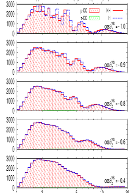
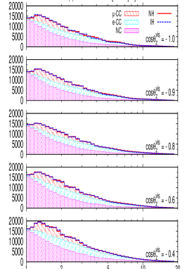
Fig. 4: Event rates, smeared by neutrino scattering together with energy and zenith angle reconstruction procedures, of (a) muon-like channel for $1-y<0.67$, (b) muon-like channel for $1-y>0.67$, and (c) cascade channel, with NH (red-solid curves) and IH (blue dashed curves) , in 1-year run of PINGU.

In Fig. 4, we show the event rates smeared by neutrino scattering and reconstruction procedures in Sec. 3.2, for both muon- and cascade channels. For the muon-like events in the panels (a) and (b), there are two sources, one from $\mu$-CC and the other from $\tau$-CC with $\tau$ decaying to $\mu$, with muon energy $E_{\mu}>1\,\mbox{GeV}$ as defined in (3.5). Those events that do not have a muon or the muon is mis-identified are all classified as cascade events in the right panel (c).

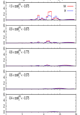
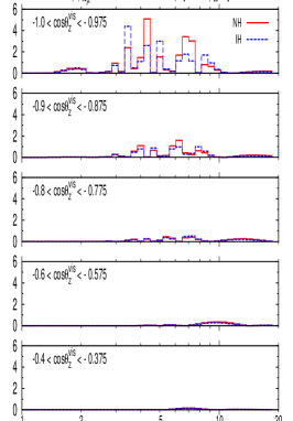
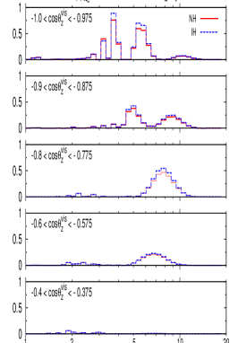
Fig. 5: Hierarchy sensitivity distribution ($\chi^{2}$ per bin), smeared by neutrino scattering together with energy and zenith angle reconstruction procedures, of (a) muon-like channel for $1-y<0.67$, (b) muon-like channel for $1-y>0.67$, and (c) cascade channel, with NH (red-solid curves) and IH (blue-dashed curves), in 1-year run of PINGU.

Let us first take a careful look at the muon-like events which mainly come from $\mu$-CC while the contribution of $\tau$-CC is almost negligible. For the large-inelasticity muon-like channel (a), the event rates drops down to zero for the energy range of $E_{\rm vis}\lesssim 1.5\,\mbox{GeV}$ with $E_{\mu}\lesssim 1\,\mbox{GeV}$. This is because of the inelasticity cut, $1-y<0.67$, and the muon energy cut, $E_{\mu}>1\,\mbox{GeV}$. On the other hand, the event rates can be nonzero in the same region for the small-inelasticity muon-like channel (b). As shown in (3.5), the neutrino energy can be exactly reconstructed for $\mu$-CC with $E_{\mu}>1\,\mbox{GeV}$ and the muon is not mis-identified. Nevertheless, the event rates are totally different from the muon-like neutrino event rates in Fig. 1, due to scattering and the zenith angle reconstruction procedure which smear away the oscillation pattern, especially in the low-energy end, $E_{\rm vis}\lesssim 2\,\mbox{GeV}$, and the horizontal region, $\cos\theta^{\rm vis}_{\rm z}\gtrsim-0.5$. Of these two channels, the small-inelasticity muon-like channel (b) has larger event rates, from which more sensitivity to the neutrino mass hierarchy can be expected.

For the cascade events, the largest component comes from NC which carries no information of neutrino oscillation and hence serves as background, while the signal comes from the $e$-CC and $\mu$-CC events. In $e$-CC, there are not so much oscillation behavior in the first place as shown in Fig. 1. The $\mu$-CC contribution mainly comes from the mis-identified muon with $E_{\mu}\lesssim 1\,\mbox{GeV}$ and hence concentrates in the low-energy end, $E_{\rm vis}\lesssim 3\,\mbox{GeV}$. We can expect the $\mu$–CC contribution to the energy range, $E_{\rm vis}\gtrsim 3\,\mbox{GeV}$, to increase with the muon mis-identification rate for $E_{\mu}>1\,,\mbox{GeV}$. Note that the contribution of $\tau$-CC is also negligible.

To make the hierarchy sensitivity explicit, we show the $\chi^{2}$ distribution in Fig. 5. For all three channels, there is almost no sensitivity in the energy range of $E_{\rm vis}\lesssim 3\,\mbox{GeV}$ or $E_{\rm vis}\gtrsim 10\,\mbox{GeV}$. The contribution from the cascade channel can extend slightly further into the high-energy end. Of the two muon-like channels, the large-inelasticity one (a) has smaller contribution than the small-inelasticity one (b) due to lower statistics. Although the cascade channel has smaller sensitivity per bin, its contribution extends from the core region ($\cos\theta^{\rm vis}_{\rm z}\lesssim-0.84$) to the mantle region ($\cos\theta^{\rm vis}_{\rm z}\gtrsim-0.84$), while the contribution from the muon-like channels damps quickly and can only span the mantle region. Consequently, the total contribution from the cascade channel can be comparable with that from the muon-like channels.

4 Energy and Angular Resolutions

Smearing effect not only comes from neutrino scattering and the reconstruction procedures as described in Sec. 3, but comes also from the detector resolutions of the reconstructed observables. The actually measured value of an observable is distributed randomly around its true value according to the corresponding resolution function. In this section, we analysis the basic features of energy and angular resolutions in Sec. 4.1 and Sec. 4.2, respectively. Their effects on the event rates and sensitivity distribution will be shown in Sec. 4.3.

4.1 Energy Resolution

The Cherenkov light produced by final-state particles can only be partially collected by the PINGU detector. The effective area with 40-string configuration is around $10m^{2}$ per megaton, in contrast to the huge size of a megaton detector which is of the characteristic scale $100m$ with typical coverage around $(4\pi/3\sim 6)\times(100m)^{2}$ where $4\pi/3$ corresponds to sphere and $6$ to cubic. A reasonable estimation of the coverage is $5\times(100m)^{2}$ per megaton. The fraction of photons that can be collected is proportional to the effective area and can be roughly estimated as the ratio between the effective area and the coverage. In other words, about $2\times 10^{-4}$ of the photons can be collected by the detection modules and most of them escape. Typically, $1\,\mbox{GeV}$ energy can produce approximately $1.8\times 10^{5}$ Cherenkov photons. With a rate of $2\times 10^{-4}$ detection, only $36$ photons can be collected. The energy fluctuation is around $\delta E/E\sim 1/6$ for $1\,\mbox{GeV}$. To be conservative, we assume the energy resolution to be,

$$\sigma_{\rm E}\approx 0.2\mbox{ GeV}\times\sqrt{E/\mbox{GeV}}\,.$$ (4.1)

This applies to both $E_{\mu}$ and $E_{\rm cas}$ in (3.5),

$$\mathbb{P}(E|E^{\prime})=\frac{1}{\sqrt{2\pi}\sigma_{E}}\exp\left[-\frac{1}{2}\left(\frac{E^{\prime}-E}{\sigma_{E}}\right)^{2}\right]\,,$$ (4.2)

separately. Due to this, the reconstructed neutrino energy for the muon-like events has a distribution around its true value. By comparing (4.1) with the oscillation period of $N^{(0)}_{\mu}$ shown in Fig. 1, we can see that the energy resolution is larger than neutrino oscillation period in the energy range of $E_{\nu}\lesssim 2\,\mbox{GeV}$. Those pattern below $2\,\mbox{GeV}$ can not survive even if smearing only comes from detector resolution.

Note that, the energy resolution presented in [45] scales as $\sigma_{\rm E}\sim 0.25\mbox{ GeV}\times(E_{\nu}/\mbox{GeV})$ for neutrino energy. This is a combination of the smearing effect due to detector resolution discussed here and the one from energy reconstruction procedure elaborated in Sec. 3.2.1. The latter has a linear scaling behavior and dominates in the high-energy end. Note that this only applies to the cascade channel. Since the muon- and cascade events have different energy reconstruction procedures, the total energy resolution is different. For muon-like events, only the detector resolution contributes while it is a combination for the cascade events. Between neutrino and antineutrino events, difference can also appear. A rigorous full-detector simulation is needed in this regard.

4.2 Angular Resolution

If muon leaves a clear track in the PINGU detector, its direction can be reconstructed with very good precision. Nevertheless, the track can be overwhelmed by the spherical cascade radiation if muon takes away only a small part of the neutrino energy. We presumably take this criterion at $1-y_{\mu}\sim 0.2$ below which the angular resolution is 50% larger than the one above it. The same thing also applies to those events with an electron. Since the radiation from electron is not so directed as the muon track and is only slightly better than the radiation from hadronic shower, the criterion is placed at higher energy ratio $1-y_{\rm e}\sim 0.4$ below which the angular resolution is assigned to be 50% larger than the one above it. In addition, the angular resolution of electron is assigned to be one time larger than that of muon. For NC events which does not have a lepton at all and those events that lepton energy is too small to be recognized, the angular resolution is much worse. As a rough approach, we use the angular distribution of CC-channel leptons with energy below $1\,\mbox{GeV}$ as their angular resolution. These are summarized below,

$$\sigma_{\theta}=\begin{cases}1.0\times 15^{\circ}\times(E_{\mu}/\mbox{GeV})^{-0.6}\,,&E_{\mu}>1\,\mbox{GeV},1-y_{\mu}>0.2\\ 1.5\times 15^{\circ}\times(E_{\mu}/\mbox{GeV})^{-0.6}\,,&E_{\mu}>1\,\mbox{GeV},1-y_{\mu}<0.2\\ 2.0\times 15^{\circ}\times(E_{\rm e}/\mbox{GeV})^{-0.6}\,,&E_{\rm e}>1\,\mbox{GeV},1-y_{\rm e}>0.2\\ 3.0\times 15^{\circ}\times(E_{\rm e}/\mbox{GeV})^{-0.6}\,,&E_{\rm e}>1\,\mbox{GeV},1-y_{\rm e}<0.2\\ \mathbb{P}(\theta^{\ell}_{\rm z})|_{E_{\ell}<1\,\mbox{\tiny GeV}},&E_{\ell}<1\,\mbox{GeV},NC,\tau-CC\mbox{ with }\tau\rightarrow\mbox{hadrons}\,.\end{cases}$$ (4.3)

The kinematics of the smearing from angular resolution takes exactly the same form as the kinematics of the smearing from neutrino scattering, shown in Fig. 3. The only modification is $\vec{P}_{\nu}\rightarrow\vec{P}_{\rm vis}$ and $\vec{P}_{\rm vis}\rightarrow\vec{P}^{\prime}_{\rm vis}$ where $\rm P^{\prime}_{\rm vis}$ is the actually measured visible momentum. They can be parametrized as,

$$-\vec{P}_{\rm vis}\equiv\left|\vec{P}_{\rm vis}\right|\left\lgroup\begin{matrix}\sin\delta\theta\\ 0\\ \cos\delta\theta\end{matrix}\right\rgroup\,,\qquad-\vec{P}^{\prime}_{\rm vis}\equiv\left|\vec{P}^{\prime}_{\rm vis}\right|\left\lgroup\begin{matrix}\sin\delta\theta^{\prime}\cos\phi^{\prime}_{\rm vis}\\ \sin\delta\theta^{\prime}\sin\phi^{\prime}_{\rm vis}\\ \cos\delta\theta^{\prime}\end{matrix}\right\rgroup\,,$$ (4.4)

in the neutrino frame where $\vec{P}_{\nu}$ aligns with the $z$-axis. Note that $\delta\theta$ is the opening angle between $\vec{P}_{\nu}$ and $\vec{P}_{\rm vis}$, determined by the neutrino scattering. Here, the opening angle $\delta\Theta$ between $\vec{P}_{\rm vis}$ and $\vec{P}^{\prime}_{\rm vis}$ distributes according to detector resolution,

$$\mathbb{P}(\delta\Theta)=\frac{\sin\delta\Theta}{N(\sigma_{\theta})}\exp\left[-\frac{1}{2}\left(\frac{\delta\Theta}{\sigma_{\theta}}\right)^{2}\right]\,,$$ (4.5)

where $N(\theta_{\theta})$ is the normalization factor. For the azimuthal angle $\phi^{\prime}$ of $\vec{P}^{\prime}_{\rm vis}$ around $\vec{P}_{\rm vis}$, it is randomly distributed in the allowed range $[0,2\pi]$. This is a simplified approach since the geometry of the PINGU detector is not isotropic and hence the angular resolution should have direction dependence. Nevertheless, the full-detector specification is not available yet, and we adopt this simple approximation. We find that, the main contribution to angular smearing comes from the zenith angle reconstruction procedure discussed in Sec. 3.2.2. Therefore, simplification in the detector angular resolution is not expected to introduce a significant bias.

Now the conversion formula (3.8) reads,

$$\cos\delta\theta^{\prime}=\cos\delta\theta\cos\delta\Theta-\sin\delta\theta\sin\delta\Theta\cos\phi^{\prime}\,.$$ (4.6)

For a given $\delta\theta$ between $\vec{P}_{\rm vis}$ and $\vec{P}_{\nu}$ as shown in Fig. 3, the measured visible momentum $\vec{P}^{\prime}_{\rm vis}$ after the detector resolution has the $\delta\theta^{\prime}$ distribution,

$$\mathbb{P}(\delta\theta|\delta\theta^{\prime})=\frac{1}{2\pi}\int\frac{\mathbb{P}(\delta\Theta)\sin\delta\theta^{\prime}}{\sqrt{\sin^{2}\delta\theta\sin^{2}\delta\Theta-(\cos\delta\theta\cos\delta\Theta-\cos\delta\theta^{\prime})^{2}}}d\delta\Theta\,,$$ (4.7)

around $\vec{P}_{\nu}$.

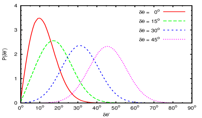
Fig. 6: Illustration of transferring angular resolution with $\sigma_{\theta}=15^{\circ}$ from the $\vec{P}_{\rm vis}$ frame to the $\vec{P}_{\nu}$ frame.

As an illustration, we show $\mathbb{P}(\delta\theta|\delta\theta^{\prime})$ for different values of $\delta\theta$ in Fig. 6. For $\delta\theta=0^{\circ}$, the measured angular distribution resembles the original form, namely $\mathbb{P}(0^{\circ}|\delta\theta^{\prime})=\mathbb{P}(\delta\theta^{\prime})$, as indicated by (4.6) which becomes $\cos\delta\theta^{\prime}=\cos\delta\Theta$ and hence $\delta\theta^{\prime}=\delta\Theta$ under this extreme circumstance.

4.3 Combined Effects

After including the effects of energy and angular resolutions, the observed event rates (3.13) become,

$$\frac{\partial^{2}N[E^{\prime}_{\rm vis},(\theta^{\rm vis}_{\rm z})^{\prime}]}{\partial E^{\prime}_{\rm vis}\partial\cos(\theta^{\rm vis}_{\rm z})^{\prime}}=\int\frac{\partial^{2}N(E_{\nu},\theta^{\nu}_{\rm z})}{\partial E_{\nu}\partial\cos\theta^{\nu}_{\rm z}}\frac{\mathbb{T}(E_{\nu}|E_{\rm vis},\delta\theta)\mathbb{P}(E_{\mu}|E^{\prime}_{\mu})\mathbb{P}(E_{\rm cas}|E^{\prime}_{\rm cas})\mathbb{P}(\delta\theta|\delta\theta^{\prime})dE_{\mu}dE_{\rm cas}d\delta\theta d\delta\theta^{\prime}}{2\pi\sqrt{\sin^{2}\theta^{\nu}_{\rm z}\sin^{2}\delta\theta^{\prime}-[\cos\theta^{\nu}_{\rm z}\cos\delta\theta^{\prime}-\cos(\theta^{\rm vis}_{\rm z})^{\prime}]^{2}}}dE_{\nu}d\cos\theta^{\nu}_{\rm z}\,,$$ (4.8)

where $E^{\prime}_{\rm vis}$ and $(\theta^{\rm vis}_{\rm z})^{\prime}$ are the actually measured visible energy and zenith angle. Note that there are two energy resolution functions, one for muon and the other for cascade, since they can be separated. The observed event rates have been shown in Fig. 7. For comparison, the same scale and format as Fig. 4 are adopted.

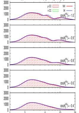
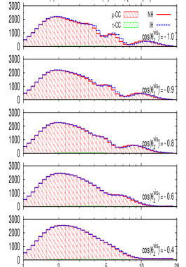
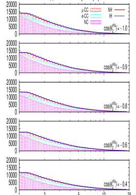
Fig. 7: Event rates, fully smeared by neutrino scattering, energy and zenith angle reconstruction procedures, as well as energy and angular resolutions, of (a) muon-like channel for $1-y<0.67$, (b) muon-like channel for $1-y>0.67$, and (c) cascade channel, with NH (red-solid curves) and IH (blue-dashed curves), in 1-year run of PINGU.

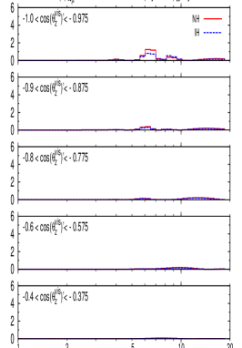
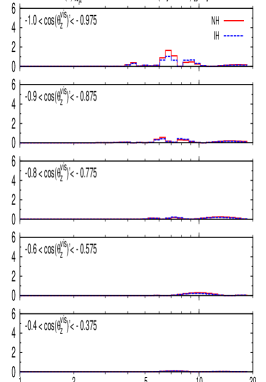
Fig. 8: Hierarchy sensitivity distribution ($\chi^{2}$ per bin), fully smeared by neutrino scattering, energy and zenith angle reconstruction procedures, as well as energy and angular resolutions, of (a) muon-like channel for $1-y<0.67$, (b) muon-like channel for $1-y>0.67$, and (c) cascade channel, with NH (red-solid curves) and IH (blue-dashed curves), in 1-year run of PINGU.

By comparing with Fig. 4, it needs to be noticed that the tail at the low-energy end extends to even lower energy due to smearing, especially for the muon-like events for $1-y<0.67$. In addition, the shape becomes much smoother, as expected, making the sensitivity to the neutrino mass hierarchy vanish in the energy range of $E^{\prime}_{\rm vis}\lesssim 4\,\mbox{GeV}$. We can see that folding with energy and angular resolutions does not change the event rates much, indicating that the smearing effect is dominated by neutrino scattering and reconstruction procedures discussed in Sec. 3.

To make the difference clearly, the counterpart of Fig. 5 is shown in Fig. 8. For comparison, the scale and format are kept the same. We can see that the sensitivity to the neutrino mass hierarchy becomes much smaller after folding with the energy and angular resolutions. No sensitivity in the region of $E^{\prime}_{\rm vis}\lesssim 4\,\mbox{GeV}$ or $\cos(\theta^{\rm vis}_{\rm z})^{\prime}\gtrsim-0.4$ survives. The sensitive region of the cascade events can still extends to mantle, but the muon-like events only have sensitivity in the core.

From these observations, we can expect that energy and angular resolutions reduce the sensitivity to the neutrino mass hierarchy, but it cannot be as large as the reduction due to neutrino scattering and reconstruction procedures.

5 $\chi^{2}$ Minimization

To be consistent with our first paper [39], which is based on event rates at the neutrino level, we introduce the same conventional $\chi^{2}$ technique,

$$\chi^{2}\equiv\sum_{\alpha}\sum_{ij}(\Delta E^{\prime}_{\rm vis})_{i}[\Delta\cos(\theta^{\rm vis}_{\rm z})^{\prime}]_{j}\left\{\dfrac{\left[\dfrac{\partial^{2}N_{\alpha}}{\partial E^{\prime}_{\rm vis}\partial\cos(\theta^{\rm vis}_{\rm z})^{\prime}}\right]^{\rm{th}}_{ij}-\left[\dfrac{\partial^{2}N_{\alpha}}{\partial E^{\prime}_{\rm vis}\partial\cos(\theta^{\rm vis}_{\rm z})^{\prime}}\right]^{\rm{obs}}_{ij}}{\sqrt{\left[\dfrac{\partial^{2}N_{\alpha}}{\partial E^{\prime}_{\nu}\partial\cos(\theta^{\rm vis}_{\rm z})^{\prime}}\right]^{\rm{obs}}_{ij}}}\right\}^{2}+\chi^{2}_{\rm{para}}\,,$$ (5.1)

to investigate the sensitivities to the neutrino mass hierarchy, the atmospheric mixing angle $\theta_{\rm a}$ as well as its octant. The first term accounts for the statistics contribution from PINGU, including three channels denoted by $\alpha$, the muon-like events for $1-y\gtrless 0.67$ and the cascade events. For the visible energy, $E^{\prime}_{\rm vis}$, 40 bins are assigned logarithmically in the range from $1\,\mbox{GeV}$ to $20\,\mbox{GeV}$. The zenith angle, $\cos(\theta^{\rm vis}_{\rm z})^{\prime}$ also has 40 bins with equal steps between $\cos(\theta^{\rm vis}_{\rm z})^{\prime}=-1$ and $0$. Since there is not much sensitivity for $E^{\prime}_{\rm vis}\lesssim 4\,\mbox{GeV}$ or $\cos(\theta^{\rm vis}_{\rm z})^{\prime}\gtrsim-0.4$, these regions can be cut off. The second term, $\chi^{2}_{\rm para}$, includes the external constraints on the neutrino oscillation parameters,

$$\chi^{2}_{\rm{para}} = \left[\frac{(\delta m^{2}_{\rm a})^{\rm{fit}}-\overline{\delta m^{2}_{\rm a}}}{\Delta\delta m^{2}_{\rm a}}\right]^{2}+\left[\frac{(\delta m^{2}_{\rm s})^{\rm{fit}}-\overline{\delta m^{2}_{\rm s}}}{\Delta\delta m^{2}_{\rm s}}\right]^{2}$$ (5.2)

$$+ \left[\frac{(\sin^{2}2\theta_{\rm r})^{\rm{fit}}-\overline{\sin^{2}2\theta_{\rm r}}}{\Delta\sin^{2}2\theta_{\rm r}}\right]^{2}+\left[\frac{(\sin^{2}2\theta_{\rm s})^{\rm{fit}}-\overline{\sin^{2}2\theta_{\rm s}}}{\Delta\sin^{2}2\theta_{\rm s}}\right]^{2}+\left[\frac{(\sin^{2}2\theta_{\rm a})^{\rm{fit}}-\overline{\sin^{2}2\theta_{\rm a}}}{\Delta\sin^{2}2\theta_{\rm a}}\right]^{2}\,,$$

where the mass squared differences, $\delta m^{2}_{\rm a}\equiv|\delta m^{2}_{13}|$ and $\delta m^{2}_{\rm s}\equiv\delta m^{2}_{21}$, the reactor mixing angle $\theta_{\rm r}\equiv\theta_{13}$, the solar mixing angle $\theta_{\rm s}\equiv\theta_{12}$, and the atmospheric mixing angle $\theta_{\rm a}\equiv\theta_{23}$ are defined according to their physical meanings. Their current best fit values and expected uncertainties,

$$\delta m^{2}_{\rm a}=2.35\pm 0.1\times 10^{-3}\mbox{eV}^{2}\,,\qquad\delta m^{2}_{\rm s}=7.50\pm 0.2\times 10^{-5}\mbox{eV}^{2}\,,$$ (5.3a)

$$\sin^{2}2\theta_{\rm r}=0.098\pm 0.005\,,\qquad\sin^{2}2\theta_{\rm s}=0.857\pm 0.024\,,\qquad\sin^{2}2\theta_{\rm a}=0.957\pm 0.030\,.$$ (5.3b)

in the near future are taken from [4, 76, 77] as well as global fits [78, 79, 80]. Note that some uncertainties are slightly smaller than the current values because improvements from the ongoing experiments are expected before PINGU become operational.

In this section, we just consider the statistical sensitivity. The systematic errors will be discussed in Sec. 6. The observed event rates are generated with the best fit values unless stated explicitly. Then the minimum of the $\chi^{2}$ function (5.1) can be obtained by varying the six neutrino oscillation parameters, namely the two mass squared differences, the three mixing angles, and the CP phase, to fit the observed event rates. Since the coefficients of $\delta$-dependent terms are small, very slight dependence on it can be expected. In the following discussions, $\delta=0^{\circ}$ is always adopted as its true value. In the $\chi^{2}$ minimization, the parameter $\delta m^{2}_{\rm s}$ and $\theta_{\rm s}$ can not affect the result much either [81]. They are fixed at their best fit values in the $\chi^{2}$ minimization.

5.1 Sensitivity to the Neutrino Mass Hierarchy

The sensitivity to the neutrino mass hierarchy can be parametrized as,

$$\Delta\chi^{2}_{\mbox{\tiny MH}}\equiv\chi^{2}_{\rm min}(\mbox{wrong hierarchy})-\chi^{2}_{\rm min}(\mbox{true hierarchy})\,,$$ (5.4)

where true hierarchy is the hierarchy used to generated the observed event rates in (5.1) and wrong hierarchy is the opposite one. Here we just use the Asimov data set [82] corresponding to the so-called “average experiment” [83]. The statistical interpretation for such a discrete bi-value fit of mass hierarchy can be found in [84, 85, 86, 87, 88] which is a function of the $\chi^{2}$ function minimum, $\Delta\chi^{2}_{\mbox{\tiny MH}}$.

$\Delta\chi^{2}_{\mbox{\tiny MH}}$	NH (true)			IH (true)
$\bar{x}_{\rm a}$ (true)	$-0.2$	$0$	$+0.2$	$-0.2$	$0$	$+0.2$
$\nu$	163.0	174.9	141.8	100.7	109.7	96.7
	252.9	215.3	168.9	143.5	140.7	120.1
Scattering & Reconstruction	26.4	13.2	10.2	14.9	12.7	10.1
	67.3	32.2	21.3	21.2	17.9	15.4
Resolution	22.9	10.2	7.1	9.9	8.7	7.0
	44.1	17.4	9.2	14.8	13.8	10.0
$\mu$ mis-ID	20.8	9.3	6.5	9.1	8.0	6.4
	40.5	16.0	8.5	14.0	12.9	9.3
Split $\mu$ ($1-y\gtrless 0.67$)	27.1	12.6	8.1	12.8	10.9	7.9
	46.9	19.5	9.9	16.8	15.9	10.8

Table 1: Sensitivity to the neutrino mass hierarchy with muon-like events only (blue) as well as both muon-like and cascade events (red) for different true values of the atmospheric mixing angle and mass hierarchy, NH on the left and IH on the right, in 1-year run of PINGU.

To see the effect of each procedure discussed in previous sections, we show the results step by step. In the first row, the sensitivities are obtained with neutrino-level event rates, corresponding to our first paper [39]. Then, we impose the scattering and reconstruction procedures elaborated in Sec. 3.2 for the second row. The effect of energy and angular resolutions in Sec. 4 can be found in the third row. Based on this, we further consider the muon mis-identification in the fourth row. These three steps all reduce the hierarchy sensitivity to some extent. Splitting muon-like event rates according to the inelasticity distribution in Sec. 3.1 can retrieve some losses as displayed in the final row. In each case, the first sub-row in blue is obtained with only muon-like events and the second one in red with both muon-like and cascade events. Note that including the cascade events can significantly improve the hierarchy sensitivity.

For the whole structure, let us first take a look at the dependence on the true neutrino mass hierarchy. If the true hierarchy is normal, the hierarchy sensitivity is higher. This trend starts from the result with neutrino event rates [39] and can be explained by Fig. 1(a) and Fig. 7. Since the energy cut is $E^{\prime}_{\rm vis}\gtrsim 4\,\mbox{GeV}$, the neutrino events below $E_{\nu}\sim 4\,\mbox{GeV}$ do not contribute much. For the muon-like channel, the event rate with IH is larger than that with NH for most of the neutrino energy range above $4\,\mbox{GeV}$. With same difference in total event rates between NH and IH, the smaller event rates make NH more sensitive as indicated in (5.1) and shown in Fig. 8. The advantage of NH will be slightly reduced when cascade events are included in the analysis due to larger event rates with NH, see Fig. 1(b). Although neutrino scattering, reconstruction procedures, and detector resolutions can smear the event rates severely, this trend is not reversed.

For each case of NH or IH, the sensitivity depends on the true value $\bar{x}_{\rm a}$ of the atmospheric mixing angle, which has been assigned three values, $\pm 0.2$ and $0$. As argued in Sec. 2, the quadratic term of $x_{\rm a}$ can dominate in the energy range $5\,\mbox{GeV}\lesssim E_{\nu}\lesssim 10\,\mbox{GeV}$ when $\bar{x}_{\rm a}=\pm 0.2$ and its contribution to the hierarchy sensitivity is destructive. This feature can modify the expected monotonic dependence on $\bar{x}_{\rm a}$ with only the linear term is considered. These observation are supported by the results in the first row of Table 1. With NH, the sensitivity is larger for $\bar{x}_{\rm a}=-0.2$ than for $\bar{x}_{\rm a}=0.2$ since the quadratic term is the same but the linear term reduces the hierarchy sensitivity when $\bar{x}_{\rm a}$ increases. With $\bar{x}_{\rm a}$ switching from $0$ to $-0.2$, the sensitivity decreases since the quadratic term can reduce the difference between NH and IH. This trend also applies to the case with IH. When the cascade channel is also included, the difference between $\bar{x}_{\rm a}=-0.2$ and $\bar{x}_{\rm a}=+0.2$ becomes larger. Naively thinking, an opposition sign between the coefficients $N^{(1)}_{\mu}$ and $N^{(1)}_{\rm e}$ of the linear term of $x_{\rm a}$ can reduce the difference between $\bar{x}_{\rm a}=-0.2$ and $\bar{x}_{\rm a}=+0.2$ when cascade events are included in the analysis, in contrast to the results shown in Table 1. The reason is, for cascade events, the contribution from the linear term of $x_{\rm a}$ is relatively larger and itself has significant dependence on the mass hierarchy. With a negative $\bar{x}_{\rm a}$, $N^{(1)}_{\rm e}$ not only increases the total event rates, but more importantly enhances the difference between NH and IH. Another thing that should be noticed is, after including the cascade events, the monotonic dependence on $\bar{x}_{\rm a}$ appears. This is because the quadratic term only comes from the muon-like events. When cascade events is included, the parameter region in which the quadratic term dominates can be avoided in $\chi^{2}$ minimization.

After neutrino scattering and reconstruction procedures are applied, the sensitivity drops significantly, by roughly an order, as expected. The reduction in the contribution from the muon-like events is more severe than the cascade events. This is because the muon-like event rates have more oscillation pattern and the smearing effect is more significant than the cascade event rates, as shown in Fig. 1. For the input value $\bar{x}_{\rm a}$ of the atmospheric mixing angle, monotonic dependence is restored even for the results with only muon-like events since after smearing the quadratic term of $x_{\rm a}$ is no longer important across the whole energy range.

The energy and angular resolutions can further reduce the sensitivity, but the reduction is not so significantly. This is because the larger smearing effect comes from the neutrino scattering and incomplete reconstruction procedures. For muon mis-identification, the reduction is not significant either since the mis-identified muon-like events still carry the information of neutrino mass hierarchy and contribute to the cascade events.

By splitting the muon-like events into two channels with the criterion, $1-y\gtrless 0.67$, the sensitivity can be significantly increased by a factor of $13\%\sim 40\%$, consisent with [42]. It can compensate the sensitivity reduction due to detector resolutions and muon mis-identification for muon-like events.

5.2 Precision on the Atmospheric Mixing Angle

To obtain the precision on the atmospheric mixing angle $\theta_{\rm a}$, we replace its external constraint, namely the last term in (5.2), by

$$\left[\frac{\left(\sin^{2}2\theta_{\rm a}\right)^{\rm fit}-\overline{\sin^{2}2\theta_{\rm a}}}{\Delta\sin^{2}2\theta_{\rm a}}\right]^{2}\rightarrow\left[\frac{x^{2}_{\rm a}-\bar{x}^{2}_{\rm a}}{0.03}\right]^{2}\,,$$ (5.5)

in order to avoid artificial contribution from the assumed true value of the atmospheric mixing angle. In other words, we keep the $1\,\sigma$ error of the present constraint in (5.3) around the input values instead of the best fit value. For each true value $\bar{x}_{\rm a}$, the $\chi^{2}$ minimization is carried out by fixing the fitting parameter $x_{\rm a}$. The resultant $\chi^{2}_{\rm min}(x_{\rm a})$ is hence a function of the fitting parameter $x_{\rm a}$, from which the precision on $x_{\rm a}$ can be determined [39]. In Table 2 we shown the results.

$\Delta(x_{\rm a})$	NH (true)			IH (true)
$\bar{x}_{\rm a}$ (true)	$-0.2$	$0$	$+0.2$	$-0.2$	$0$	$+0.2$
$\nu$	0.014	0.036	0.011	0.014	0.046	0.011
	0.012	0.025	0.010	0.012	0.035	0.011
Scattering & Reconstruction	0.025	0.051	0.015	0.024	0.073	0.017
	0.020	0.039	0.014	0.022	0.061	0.016
Resolution	0.027	0.055	0.016	0.025	0.077	0.018
	0.021	0.043	0.016	0.024	0.067	0.018
$\mu$ mis-ID	0.028	0.059	0.017	0.026	0.078	0.019
	0.022	0.045	0.017	0.025	0.070	0.019
Split $\mu$ ($1-y\gtrless 0.67$)	0.027	0.057	0.017	0.026	0.077	0.019
	0.022	0.045	0.016	0.024	0.068	0.019

Table 2: Precision on the atmospheric mixing angle for muon-like events only (blue) as well as both muon-like and cascade events (red) for different true values of the atmospheric mixing angle and mass hierarchy, NH on the left and IH on the right, in 1-year run of PINGU.

As demonstrated in [39], the precision $\Delta(x_{\rm a})$ is mainly dictated by the combined coefficients, $N^{(1)}_{\mu}+2\bar{x}_{\rm a}N^{(5)}_{\mu}$, where $\bar{x}_{\rm a}$ is the input (true) value of the atmospheric mixing angle. Since $N^{(5)}_{\mu}$ is much larger than $N^{(1)}_{\mu}$ as shown in Fig. 1, the second term dominates for $\bar{x}_{\rm a}=\pm 0.2$, leading to comparable precisions for $\bar{x}_{\rm a}=-0.2$ and $\bar{x}_{\rm a}=+0.2$ with small difference due to the first term $N^{(1)}_{\mu}$. For all cases, the precision with vanishing $\bar{x}_{\rm a}$ is the largest since the second term $2\bar{x}_{\rm a}N^{(5)}_{\mu}$ vanishes. This pattern remains even after the cascade events are included, but slightly reduced. Including cascade events can help to enhance the precision on $x_{\rm a}$, especially when it is small, $\bar{x}_{\rm a}\approx 0$.

Of the three steps applied to the neutrino event rates, neutrino scattering and reconstruction procedures have the largest impact on reducing the precision on $x_{\rm a}$. It is quite stable when muon-like events are split into two parts, and when detector resolutions and muon mis-identification are imposed.

5.3 Sensitivity to the Octant of the Atmospheric Mixing Angle

$\Delta\chi^{2}_{\mbox{\tiny Octant}}$	NH (true)				IH (true)
$\bar{x}_{\rm a}$ (true)	$-0.2$	$-0.1$	$+0.1$	$+0.2$	$-0.2$	$-0.1$	$+0.1$	$+0.2$
$\nu$	41.5	6.7	20.6	64.1	10.3	2.9	4.1	12.9
	84.8	15.1	29.3	162.6	32.5	8.0	12.0	46.0
Scattering & Reconstruction	24.4	3.1	9.6	47.7	7.5	1.8	2.8	9.9
	36.9	6.2	13.2	103.0	15.6	3.3	5.5	21.4
Resolution	20.4	2.6	8.3	43.4	6.3	1.4	2.5	8.8
	27.9	4.4	10.2	76.2	11.1	2.3	4.1	15.4
$\mu$ mis-ID	18.6	2.4	7.5	39.2	5.7	1.3	2.2	7.9
	25.9	4.1	9.2	69.9	10.3	2.1	3.7	14.3
Split $\mu$ ($1-y\gtrless 0.67$)	19.6	2.5	7.8	40.4	6.6	1.5	2.5	8.7
	26.9	4.2	9.5	70.9	11.2	2.3	4.0	15.1

Table 3: Sensitivity to the octant of the atmospheric mixing angle for muon-like events only (blue) as well as both muon-like and cascade events (red) for different true values of the atmospheric mixing angle and mass hierarchy, NH on the left and IH on the right, in 1-year run of PINGU.

The octant sensitivity can be defined just like the sensitivity to the neutrino mass hierarchy (5.4),

$$\Delta\chi^{2}_{\mbox{\tiny Octant}}\equiv|\chi^{2}_{\rm min}(\mbox{LO})-\chi^{2}_{\rm min}(\mbox{HO})|\,,$$ (5.6)

where $\chi^{2}_{\rm min}(\mbox{LO})$ is obtained by limiting the fit parameter with $\theta_{\rm a}<45^{\circ}$ and $\chi^{2}_{\rm min}(\mbox{HO})$ with $\theta_{\rm a}>45^{\circ}$. The results are shown in Table 3 for four true values $\bar{x}_{\rm a}=\pm 0.2,\,\pm 0.1$. We can see that the octant sensitivity is larger if the true hierarchy is normal, due to smaller total event rates and also larger linear term coefficients $N^{(1)}_{\alpha}$ ($\alpha=\mu,{\rm e}$) with NH, and if the atmospheric angle is in the lower octant with a positive $\bar{x}_{\rm a}$. The sensitivity can be effectively reduced due to neutrino scattering and reconstruction procedures, as well as resolutions and muon mis-identification, and slightly increased after splitting the muon-like events into two channels according to the inelasticity distribution. Note that the cascade events can significantly improve the octant sensitivity.

6 Systematic Errors

In this section, we study the impacts of systematic errors in the energy and angular resolutions, the muon mis-identification rate, and the overall normalization of the flux times cross sections, to examine how each of them affects the measurement sensitivities. The impacts of combining these four systematic errors have also been studied. Note that this list of systematic uncertainties is far from complete. For instance, there can be uncertainties in neutrino/antineutrino ratios (fluxes, cross sections), event energy shape and scale, and so on. A complete survey of these systematic uncertainties is beyond the scope of this paper.

The details of the systematics we consider are listed below.

1. For the energy resolution, we keep the Gaussian form (4.1) and assign a 15% error, namely $\sigma_{\mbox{\tiny E}}=(0.2\pm 0.03)\mbox{ GeV}\times\sqrt{E/\mbox{GeV}}$.

2. For the angular resolution, any parameters in the functional form (4.3) can suffer from systematic uncertainties. According to the physical picture illustrated in Sec. 4.2, we just examine the impacts of allowing 20% uncertainty in the common resolution of $\sigma_{\theta}$, i.e., $\sigma_{\theta}=(15^{\circ}\pm 3^{\circ})\times(E/\mbox{GeV})^{-0.6}$ for the first case in (4.3) while retaining the relation between different cases.

3. The muon mis-identification rate should naively be small at high muon energies. Since full-detector simulation of the PINGU detector is not available to us, we simply consider a constant 20% error in the constant mis-identification rate, i.e., $(10\pm 2)\%$ mis-identification rate which is independent of the muon energy.

4. For the overall normalization, we assign a common 5% error for all the neutrino events, since we expect that the largest error comes from the atmospheric neutrino fluxes. Although muon- and electron-neutrino as well as anti-neutrino fluxes may each have distinct uncertainties, we expect that the relative errors to be small and the common overall normalization error dominates [89] because they have common origins. Experimentally, the normalization uncertainty can be reduced by measuring both up- and down-going neutrinos at PINGU and using down-going event rates to normalize the up-going one, or by anchoring the flux at high energies ($E_{\nu}>20\,\mbox{GeV}$) [41].

We use the so called pull method [90] to treat the systematic errors. Their impacts on the event rates can be parametrized as linear functions,

$$\frac{\partial^{2}N_{\alpha}(c_{i})}{\partial E^{\prime}_{\rm vis}\partial\cos(\theta^{\rm vis}_{\rm z})^{\prime}}\approx\frac{\partial^{2}N_{\alpha}\left(c^{(0)}_{i}\right)}{\partial E^{\prime}_{\rm vis}\partial\cos(\theta^{\rm vis}_{\rm z})^{\prime}}+\sum_{i}\partial_{c_{i}}\left.\left[\frac{\partial^{2}N_{\alpha}(c_{i})}{\partial E^{\prime}_{\rm vis}\partial\cos(\theta^{\rm vis}_{\rm z})^{\prime}}\right]\right|_{c_{i}=c^{(0)}_{i}}\times\left(c_{i}-c^{(0)}_{i}\right)\,,$$ (6.1)

where $c_{i}$ parametrizes the variable with a systematic error, and $c^{(0)}_{i}$ represents the corresponding central value. This linearized approximation can hold quite well for all the four systematic errors considered here. Their effects, when imposed separately or combined, on the sensitivity to mass hierarchy, the precision on the atmospheric mixing angle, and the sensitivity to the octant, have been summarized in Table 4, Table 5, and Table 6, respectively.

$\Delta\chi^{2}_{\mbox{\tiny MH}}$	NH (true)			IH (true)
$\bar{x}_{\rm a}$ (true)	$-0.2$	$0$	$+0.2$	$-0.2$	$0$	$+0.2$
$\sigma_{\mbox{\tiny E}}=(0.2\pm 0.03)\mbox{ GeV}\times\sqrt{E/\mbox{GeV}}$	26.1	11.2	7.7	11.5	10.0	7.1
	42.3	18.0	8.6	16.0	14.8	9.9
$\sigma_{\theta}=(15^{\circ}\pm 3^{\circ})\times(E/\mbox{GeV})^{-0.6}$	26.3	11.5	7.9	11.8	9.9	7.6
	43.1	18.2	9.0	16.1	15.1	10.0
$\mu$ mis-ID ($10\%\pm 2\%$)	19.0	8.4	6.1	8.8	7.2	5.3
	42.1	17.1	8.5	15.3	13.3	9.2
Normalization ($1\pm 0.05$)	16.8	7.9	6.6	8.6	6.9	5.0
	43.6	16.9	8.7	14.0	13.8	8.7
Combined	12.6	7.5	5.9	7.5	6.2	4.8
	41.6	16.1	8.3	13.7	12.2	7.7

Table 4: The impact of systematic errors on the sensitivity to the neutrino mass hierarchy with only muon-like events (blue) as well as both muon-like and cascade events (red) for different true values of the atmospheric mixing angle and mass hierarchy, NH on the left and IH on the right, in 1-year run of PINGU.

By comparing Table 4 with Table 1, we observe that the results are quite stable under the systematic error in energy and angular resolutions as expected from the fact that the smearing effect mainly comes from the neutrino scattering together with the reconstruction procedures, and the results are not much affected by the detector resolutions in the first place. For the systematic error in the muon mis-identification rate, if only the muon-like events are used (blue), the sensitivity is significantly reduced by the 20% uncertainty. The situation becomes stable when the cascade events are also included in the analysis (red), because the mis-identified muon still carries the information of atmospheric neutrino oscillation which is not lost but contributes to the cascade events instead. The error from the overall normalization has the largest influence for muon-like events because the lower or higher flux can mimic the presence or absence of the MSW resonance in the dominant muon channel. The negative impacts can be partially recovered by including the cascade events.

$\Delta(x_{\rm a})$	NH (true)			IH (true)
$\bar{x}_{\rm a}$ (true)	$-0.2$	$0$	$+0.2$	$-0.2$	$0$	$+0.2$
$\sigma_{\mbox{\tiny E}}=(0.2\pm 0.03)\mbox{ GeV}\times\sqrt{E/\mbox{GeV}}$	0.027	0.057	0.017	0.026	0.077	0.019
	0.025	0.045	0.016	0.025	0.068	0.019
$\sigma_{\theta}=(15^{\circ}\pm 3^{\circ})\times(E/\mbox{GeV})^{-0.6}$	0.028	0.057	0.017	0.026	0.078	0.019
	0.023	0.045	0.017	0.024	0.069	0.019
$\mu$ mis-ID ($10\%\pm 2\%$)	0.028	0.069	0.021	0.028	0.083	0.024
	0.022	0.052	0.020	0.026	0.078	0.020
Normalization ($1\pm 0.05$)	0.033	0.081	0.025	0.031	0.090	0.030
	0.023	0.055	0.022	0.027	0.078	0.021
Combined	0.034	0.083	0.028	0.033	0.099	0.032
	0.026	0.058	0.024	0.029	0.081	0.023

Table 5: The impact of systematic errors on the precision of the atmospheric mixing angle $\theta_{\rm a}$ with only muon-like events (blue) as well as both muon-like and cascade events (red) for different true values of the atmospheric mixing angle and mass hierarchy, NH on the left and IH on the right, in 1-year run of PINGU.

On the other hand, comparison of Table 2 and Table 5 shows that the precision on the atmospheric mixing angle parameter $x_{\rm a}=1/2-\sin^{2}\theta_{\rm a}$ is very stable under the influence of all the systematic errors, with the only exception of the systematic error in the overall normalization when only the muon-like events are considered.

$\Delta\chi^{2}_{\mbox{\tiny Octant}}$	NH (true)				IH (true)
$\bar{x}_{\rm a}$ (true)	$-0.2$	$-0.1$	$+0.1$	$+0.2$	$-0.2$	$-0.1$	$+0.1$	$+0.2$
$\sigma_{\mbox{\tiny E}}=(0.2\pm 0.03)\mbox{ GeV}\times\sqrt{E/\mbox{GeV}}$	19.4	2.5	7.7	40.0	6.5	1.5	2.5	8.7
	26.3	4.1	9.1	65.8	10.8	2.3	3.8	14.3
$\sigma_{\theta}=(15^{\circ}\pm 3^{\circ})\times(E/\mbox{GeV})^{-0.6}$	19.3	2.5	7.7	40.2	6.6	1.5	2.5	8.7
	26.7	4.2	9.1	66.8	11.0	2.3	3.8	14.5
$\mu$ mis-ID ($10\%\pm 2\%$)	19.1	2.2	5.2	39.2	4.5	1.3	1.9	8.3
	26.5	4.0	8.2	66.1	10.8	2.0	2.7	13.8
Normalization ($1\pm 0.05$)	10.5	1.8	3.1	13.1	3.5	0.9	0.9	3.6
	26.5	4.2	9.2	70.6	11.1	2.1	3.7	14.8
Combined	9.3	1.7	2.8	12.4	3.4	0.8	0.8	3.5
	20.0	3.2	7.6	33.9	8.6	1.9	1.9	9.1

Table 6: The impact of systematic errors on the sensitivity to the octant of the atmospheric mixing angle for muon-like events only (blue) as well as both muon-like and cascade events (red) for different true values of the atmospheric mixing angle and mass hierarchy, NH on the left and IH on the right, in 1-year run of PINGU.

For the octant determination, comparison between Table 3 and Table 6 shows also that the systematic errors in energy and angular resolutions, as well as that in the muon mis-identification rate, do not significantly reduce the sensitivity. It drops significantly when the systematic error in the overall normalization is introduced, when only the muon-like events are considered. The sensitivity can be recovered again, once the cascade events are included in the analysis.

7 Conclusion

The physics reach of measuring the atmospheric neutrino oscillation pattern at PINGU to determine the neutrino mass hierarchy, the atmospheric mixing angle and its octant is explored in detail by making use of the decomposition property of the observable event rates in the propagation basis. Smearing in the reconstructed neutrino energy and the zenith angle due to the neutrino CC scattering kinematics has been carefully studied, together with the energy and angular resolutions of the detector. We find that the smearing effects reduce the sensitivity to the neutrino mass hierarchy, by one order of magnitude while the precision on the atmospheric mixing angle and sensitivity to its octant is worsened by a factor around $2$. The mass hierarchy sensitivity can increase by up to $40\%$ if the muon-like events are split into two channels with the criterion $1-y\gtrless 0.67$ by estimating the inelasticity $y$ of each event. It also improves slightly the precision on the atmospheric mixing angle and its octant determination. These benefits from the inelasticity measurement of the muon-like events can partially compensate the negative effect of detector resolutions and muon mis-identification. Including the cascade events can not only increase the sensitivity of all the measurements, but most importantly stabilize the sensitivity against the influence from systematic errors in the muon mis-identification rate and the overall flux normalization. Further improvements can be expected from detailed optimization of the muon channel splitting criterion, or even refined binning of muon inelasticity instead of splitting the muon events into just two channels, and including the down-going events as well as the high energy atmospheric neutrinos to reduce the flux uncertainties. We hope that our simple but systematic analysis will help preparing dedicated studies with full detector simulation.

8 Acknowledgements

The authors are grateful to the discussions with Francis Halzen and Carsten Rott on the PINGU detector and SFG would like to thank Costas Andreopoulos for kind help on GENIE. The Japan Society for the Promotion of Science (JSPS) has generously provided SFG a postdoc fellowship to do research at KEK, which is deeply appreciated. This work is supported in part by Grant-in-Aid for Scientific research (No. 25400287) from JSPS.

References

- [1] K. Abe et al. Indication of Electron Neutrino Appearance from an Accelerator-produced Off-axis Muon Neutrino Beam. Phys.Rev.Lett., 107:041801, 2011, [arXiv:1106.2822 [hep-ex]].
- [2] P. Adamson et al. Improved search for muon-neutrino to electron-neutrino oscillations in MINOS. Phys.Rev.Lett., 107:181802, 2011, [arXiv:1108.0015 [hep-ex]].
- [3] Y. Abe et al. Indication for the disappearance of reactor electron antineutrinos in the Double Chooz experiment. Phys.Rev.Lett., 108:131801, 2012, [arXiv:1112.6353 [hep-ex]].
- [4] P.A.N. Machado, H. Minakata, H. Nunokawa, and R. Zukanovich Funchal. Combining Accelerator and Reactor Measurements of : The First Result. JHEP, 1205:023, 2012, [arXiv:1111.3330 [hep-ph]].
- [5] F.P. An et al. Observation of electron-antineutrino disappearance at Daya Bay. Phys.Rev.Lett., 108:171803, 2012, [arXiv:1203.1669 [hep-ex]].
- [6] J.K. Ahn et al. Observation of Reactor Electron Antineutrino Disappearance in the RENO Experiment. Phys.Rev.Lett., 108:191802, 2012, [arXiv:1204.0626 [hep-ex]].
- [7] F.P. An et al. Improved Measurement of Electron Antineutrino Disappearance at Daya Bay. Chin.Phys., C37:011001, 2013, [arXiv:1210.6327 [hep-ex]].
- [8] Hisakazu Minakata. Phenomenology of future neutrino experiments with large Theta(13). Nucl.Phys.Proc.Suppl., 235-236:173–179, 2013, [arXiv:1209.1690 [hep-ph]].
- [9] D.P. Roy. Determination of the Third Neutrino-Mixing Angle and its Implications. J.Phys., G40:053001, 2013, [arXiv:1210.4712 [hep-ph]].
- [10] Silvia Pascoli and Thomas Schwetz. Prospects for Neutrino Oscillation Physics. Advances in High Energy Physics, 2013.
- [11] R.N. Cahn, D.A. Dwyer, S.J. Freedman, W.C. Haxton, R.W. Kadel, et al. White Paper: Measuring the Neutrino Mass Hierarchy. 2013, [arXiv:1307.5487 [hep-ex]].
- [12] Y. F. Wang. Presentation given at INPA Journal Club, LBNL, February, 2013.
- [13] RENO-50 Collaboration. International Workshop on RENO-50 toward Neutrino Mass Hierarchy, 2013.
- [14] D. Jason Koskinen. IceCube-DeepCore-PINGU: Fundamental neutrino and dark matter physics at the South Pole. Mod.Phys.Lett., A26:2899–2915, 2011.
- [15] K. Abe, T. Abe, H. Aihara, Y. Fukuda, Y. Hayato, et al. Letter of Intent: The Hyper-Kamiokande Experiment – Detector Design and Physics Potential. 2011, [arXiv:1109.3262 [hep-ex]].
- [16] E. Kearns et al. Hyper-Kamiokande Physics Opportunities. 2013, [arXiv:1309.0184 [hep-ex]].
- [17] Srubabati Goswami. Physics Program of the India-Based Neutrino Observatory. Neutrino Oscillation Workshop, Ortanto, Italy, September 2008.
- [18] M. Sajjad Athar et al. India-based Neutrino Observatory: Project Report. Volume I. 2006.
- [19] A. Rubbia. Experiments for CP violation: A Giant liquid argon scintillation, Cerenkov and charge imaging experiment? pages 321–350, 2004, [hep-ph/0402110].
- [20] A. Ereditato and A. Rubbia. Conceptual design of a scalable multi-kton superconducting magnetized liquid Argon TPC. Nucl.Phys.Proc.Suppl., 155:233–236, 2006, [hep-ph/0510131].
- [21] G. Battistoni, A. Ferrari, C. Rubbia, P.R. Sala, and F. Vissani. Atmospheric neutrinos in a large liquid argon detector. 2006, [hep-ph/0604182].
- [22] A. Bueno, Z. Dai, Y. Ge, M. Laffranchi, A.J. Melgarejo, et al. Nucleon decay searches with large liquid argon TPC detectors at shallow depths: Atmospheric neutrinos and cosmogenic backgrounds. JHEP, 0704:041, 2007, [hep-ph/0701101].
- [23] D.S. Ayres et al. NOvA: Proposal to build a 30 kiloton off-axis detector to study oscillations in the NuMI beamline. 2004, [hep-ex/0503053].
- [24] R.B. Patterson. The NOvA Experiment: Status and Outlook. Nucl.Phys.Proc.Suppl., 235-236:151–157, 2013, [arXiv:1209.0716 [hep-ex]].
- [25] C. Adams et al. Scientific Opportunities with the Long-Baseline Neutrino Experiment. 2013, [arXiv:1307.7335 [hep-ex]].
- [26] G.J. Feldman, J. Hartnell, and T. Kobayashi. Long-baseline neutrino oscillation experiments. Adv.High Energy Phys., 2013:475749, 2013, [arXiv:1210.1778 [hep-ex]].
- [27] P.A.N. Machado, H. Minakata, H. Nunokawa, and R. Zukanovich Funchal. What can we learn about the lepton CP phase in the next 10 years? 2013, [arXiv:1307.3248 [hep-ph]].
- [28] Y. Itow et al. The JHF-Kamioka neutrino project. pages 239–248, 2001, [hep-ex/0106019].
- [29] T. Ishida. T2HK: J-PARC upgrade plan for future and beyond T2K. 2013, [arXiv:1311.5287 [hep-ex]].
- [30] Sanjib Kumar Agarwalla, Suprabh Prakash, and S. Uma Sankar. Resolving the octant of with T2K and NOvA. JHEP, 1307:131, 2013, 1301.2574.
- [31] Andrew D. Hanlon, Shao-Feng Ge, and Wayne W. Repko. Phenomenological Study of Residual and Symmetries. 2013, [arXiv:1308.6522 [hep-ph]].
- [32] S.T. Petcov. New enhancement mechanism of the transitions in the earth of the solar and atmospheric neutrinos crossing the earth core. Nucl.Phys.Proc.Suppl., 77:93–97, 1999, [hep-ph/9809587].
- [33] M. Chizhov, M. Maris, and S.T. Petcov. On the oscillation length resonance in the transitions of solar and atmospheric neutrinos crossing the earth core. 1998, [hep-ph/9810501].
- [34] Serguey T. Petcov. The Oscillation length resonance in the transitions of solar and atmospheric neutrinos crossing the earth core. pages 219–227, 1998, [hep-ph/9811205].
- [35] M.V. Chizhov and S.T. Petcov. New conditions for a total neutrino conversion in a medium. Phys.Rev.Lett., 83:1096–1099, 1999, [hep-ph/9903399].
- [36] M.V. Chizhov and S.T. Petcov. Enhancing mechanisms of neutrino transitions in a medium of nonperiodic constant density layers and in the earth. Phys.Rev., D63:073003, 2001, [hep-ph/9903424].
- [37] Tommy Ohlsson and Hakan Snellman. Neutrino oscillations with three flavors in matter: Applications to neutrinos traversing the Earth. Phys.Lett., B474:153–162, 2000, [hep-ph/9912295].
- [38] Evgeny K. Akhmedov, Michele Maltoni, and Alexei Yu. Smirnov. 1-3 leptonic mixing and the neutrino oscillograms of the Earth. JHEP, 0705:077, 2007, [hep-ph/0612285].
- [39] Shao-Feng Ge, Kaoru Hagiwara, and Carsten Rott. Physics of Atmospheric Neutrino Oscillations with a Huge Underground Detector. 2013, [arXiv:1309.3176 [hep-ph]].
- [40] E. Kh. Akhmedov, Soebur Razzaque, and A. Yu. Smirnov. Mass hierarchy, 2-3 mixing and CP-phase with Huge Atmospheric Neutrino Detectors. JHEP, 1302:082, 2013, [arXiv:1205.7071 [hep-ph]].
- [41] D. Franco, C. Jollet, A. Kouchner, V. Kulikovskiy, A. Meregaglia, et al. Mass hierarchy discrimination with atmospheric neutrinos in large volume ice/water Cherenkov detectors. JHEP, 1304:008, 2013, [arXiv:1301.4332 [hep-ex]].
- [42] Mathieu Ribordy and Alexei Yu Smirnov. Improving the neutrino mass hierarchy identification with inelasticity measurement in PINGU and ORCA. Phys.Rev., D87:113007, 2013, [arXiv:1303.0758 [hep-ph]].
- [43] Walter Winter. Neutrino mass hierarchy determination with IceCube-PINGU. Phys.Rev., D88:013013, 2013, [arXiv:1305.5539 [hep-ph]].
- [44] Mattias Blennow and Thomas Schwetz. Determination of the neutrino mass ordering by combining PINGU and Daya Bay II. JHEP, 1309:089, 2013, [arXiv:1306.3988 [hep-ph]].
- [45] Andreas Grob, in behalf of the IceCube Collaboration. 33rd International Cosmic Ray Conference, Rio De Janeiro, 2013.
- [46] M.G. Aartsen et al. PINGU Sensitivity to the Neutrino Mass Hierarchy. 2013, [arXiv:1306.5846 [astro-ph.IM]].
- [47] Animesh Chatterjee, Pomita Ghoshal, Srubabati Goswami, and Sushant K. Raut. Octant sensitivity for large in atmospheric and long baseline neutrino experiments. JHEP, 1306:010, 2013, [arXiv:1302.1370 [hep-ph]].
- [48] Sandhya Choubey and Anushree Ghosh. Determining the Octant of with PINGU, T2K, NOvA and Reactor Data. 2013, [arXiv:1309.5760 [hep-ph]].
- [49] Tommy Ohlsson, He Zhang, and Shun Zhou. Probing the leptonic Dirac CP-violating phase in neutrino oscillation experiments. Phys.Rev., D87(5):053006, 2013, [arXiv:1301.4333 [hep-ph]].
- [50] S.T. Petcov. An Analytic Description of Three Neutrino Oscillations in Matter With Varying Density. Phys.Lett., B214:259, 1988.
- [51] Evgeny K. Akhmedov, A. Dighe, P. Lipari, and A.Y. Smirnov. Atmospheric neutrinos at Super-Kamiokande and parametric resonance in neutrino oscillations. Nucl.Phys., B542:3–30, 1999, [hep-ph/9808270].
- [52] Hidekazu Yokomakura, Keiichi Kimura, and Akira Takamura. Overall feature of CP dependence for neutrino oscillation probability in arbitrary matter profile. Phys.Lett., B544:286–294, 2002, [hep-ph/0207174].
- [53] A.M. Dziewonski and D.L. Anderson. Preliminary reference earth model. Phys.Earth Planet.Interiors, 25:297–356, 1981.
- [54] M. Sajjad Athar, M. Honda, T. Kajita, K. Kasahara, and S. Midorikawa. Atmospheric neutrino flux at INO, South Pole and Pyhásalmi. Phys.Lett., B718:1375–1380, 2013, [arXiv:1210.5154 [hep-ph]].
- [55] H. Gallagher. The NEUGEN neutrino event generator. Nucl.Phys.Proc.Suppl., 112:188–194, 2002.
- [56] Jian Tang and Walter Winter. Requirements for a New Detector at the South Pole Receiving an Accelerator Neutrino Beam. JHEP, 1202:028, 2012, [arXiv:1110.5908 [hep-ph]].
- [57] L. Wolfenstein. Neutrino Oscillations in Matter. Phys.Rev., D17:2369–2374, 1978.
- [58] S.P. Mikheev and A. Yu. Smirnov. Resonance Amplification of Oscillations in Matter and Spectroscopy of Solar Neutrinos. Sov.J.Nucl.Phys., 42:913–917, 1985, [Yad.Fiz. 42 (1985) 1441-1448].
- [59] S.P. Mikheev and A. Yu. Smirnov. Resonant amplification of neutrino oscillations in matter and solar neutrino spectroscopy. Nuovo Cim., C9:17–26, 1986.
- [60] Vernon D. Barger, K. Whisnant, S. Pakvasa, and R.J.N. Phillips. Matter Effects on Three-Neutrino Oscillations. Phys.Rev., D22:2718, 1980.
- [61] Q.Y. Liu and A. Yu. Smirnov. Neutrino mass spectrum with muon-neutrino, sterile-neutrino oscillations of atmospheric neutrinos. Nucl.Phys., B524:505–523, 1998, [hep-ph/9712493].
- [62] Q.Y. Liu, S.P. Mikheyev, and A. Yu. Smirnov. Parametric resonance in oscillations of atmospheric neutrinos? Phys.Lett., B440:319–326, 1998, [hep-ph/9803415].
- [63] Evgeny K. Akhmedov. Parametric resonance of neutrino oscillations and passage of solar and atmospheric neutrinos through the earth. Nucl.Phys., B538:25–51, 1999, [hep-ph/9805272].
- [64] Evgeny K. Akhmedov, A. Dighe, P. Lipari, and A.Y. Smirnov. Atmospheric neutrinos at Super-Kamiokande and parametric resonance in neutrino oscillations. Nucl.Phys., B542:3–30, 1999, [hep-ph/9808270].
- [65] M. Maris and S.T. Petcov. A Study of the day-night effect for the Super-Kamiokande detector: 2. Electron spectrum deformations and day-night asymmetries. Phys.Rev., D56:7444–7455, 1997, [hep-ph/9705392].
- [66] Q.Y. Liu, M. Maris, and S.T. Petcov. A Study of the day-night effect for the Super-Kamiokande detector: 1. Time averaged solar neutrino survival probability. Phys.Rev., D56:5991–6002, 1997, [hep-ph/9702361].
- [67] S.T. Petcov. Diffractive - like (or parametric resonance - like?) enhancement of the earth (day-night) effect for solar neutrinos crossing the earth core. Phys.Lett., B434:321–332, 1998, [hep-ph/9805262].
- [68] Raj Gandhi, Chris Quigg, Mary Hall Reno, and Ina Sarcevic. Ultrahigh-energy neutrino interactions. Astropart.Phys., 5:81–110, 1996, [hep-ph/9512364].
- [69] Raj Gandhi, Chris Quigg, Mary Hall Reno, and Ina Sarcevic. Neutrino interactions at ultrahigh-energies. Phys.Rev., D58:093009, 1998, [hep-ph/9807264].
- [70] C. Andreopoulos, A. Bell, D. Bhattacharya, F. Cavanna, J. Dobson, et al. The GENIE Neutrino Monte Carlo Generator. Nucl.Instrum.Meth., A614:87–104, 2010, [arXiv:0905.2517 [hep-ph]].
- [71] M. Ribordy. Methods and problems in neutrino observatories. 2012, [arXiv:1205.4965 [astro-ph]].
- [72] Mathieu Ribordy. Reconstruction of Composite Events in Neutrino Telescopes. Nucl.Instrum.Meth., A574:137–143, 2007, [astro-ph/0611604].
- [73] Marek Kowalski. On the reconstruction of cascade-like events in the AMANDA detector. 2000.
- [74] Marek Paul Kowalski. Search for neutrino induced cascades with the AMANDA-II detector. 2004.
- [75] Leif Radel and Christopher Wiebusch. Calculation of the Cherenkov light yield from electromagnetic cascades in ice with Geant4. Astropart.Phys., 44:102–113, 2013, [arXiv:1210.5140 [astro-ph.IM]].
- [76] Giles Barr, in behalf of the MINOS Collaboration. ICHEP 2012, July, Melbourne.
- [77] Beringer et al. Review of particle physics. Phys. Rev. D, 86:010001, Jul 2012.
- [78] D.V. Forero, M. Tortola, and J.W.F. Valle. Global status of neutrino oscillation parameters after Neutrino-2012. Phys.Rev., D86:073012, 2012, [arXiv:1205.4018 [hep-ph]].
- [79] G.L. Fogli, E. Lisi, A. Marrone, D. Montanino, A. Palazzo, et al. Global analysis of neutrino masses, mixings and phases: entering the era of leptonic CP violation searches. Phys.Rev., D86:013012, 2012, [arXiv:1205.5254 [hep-ph]].
- [80] M.C. Gonzalez-Garcia, Michele Maltoni, Jordi Salvado, and Thomas Schwetz. Global fit to three neutrino mixing: critical look at present precision. JHEP, 1212:123, 2012, [arXiv:1209.3023 [hep-ph]].
- [81] Anushree Ghosh, Tarak Thakore, and Sandhya Choubey. Determining the Neutrino Mass Hierarchy with INO, T2K, NOvA and Reactor Experiments. JHEP, 1304:009, 2013, [arXiv:1212.1305 [hep-ph]].
- [82] G. Cowan, K. Cranmer, E. Gross, and O. Vitells. Asymptotic formulae for likelihood-based tests of new physics. European Physical Journal C, 71:1554, February 2011, [arXiv:1007.1727 [physics.data-an]].
- [83] Thomas Schwetz. What is the probability that theta(13) and CP violation will be discovered in future neutrino oscillation experiments? Phys.Lett., B648:54–59, 2007, [hep-ph/0612223].
- [84] X. Qian, A. Tan, W. Wang, J.J. Ling, R.D. McKeown, et al. Statistical Evaluation of Experimental Determinations of Neutrino Mass Hierarchy. Phys.Rev., D86:113011, 2012, [arXiv:1210.3651 [hep-ph]].
- [85] Shao-Feng Ge, Kaoru Hagiwara, Naotoshi Okamura, and Yoshitaro Takaesu. Determination of mass hierarchy with medium baseline reactor neutrino experiments. JHEP, 1305:131, 2013, [arXiv:1210.8141 [hep-ph]].
- [86] Emilio Ciuffoli, Jarah Evslin, and Xinmin Zhang. Sensitivity to the Neutrino Mass Hierarchy. 2013, [arXiv:1305.5150 [hep-ph]].
- [87] Mattias Blennow, Pilar Coloma, Patrick Huber, and Thomas Schwetz. Quantifying the sensitivity of oscillation experiments to the neutrino mass ordering. 2013, [arXiv:1311.1822 [hep-ph]].
- [88] Mattias Blennow. On the Bayesian approach to neutrino mass ordering. 2013, [arXiv:1311.3183 [hep-ph]].
- [89] Todor Stanev. Atmospheric neutrino challenges. Nucl.Phys.Proc.Suppl., 145:69–74, 2005, [astro-ph/0412395].
- [90] G.L. Fogli, E. Lisi, A. Marrone, D. Montanino, and A. Palazzo. Getting the most from the statistical analysis of solar neutrino oscillations. Phys.Rev., D66:053010, 2002, [hep-ph/0206162].