A Generic Position Based Method for Real Root Isolation of Zero-Dimensional Polynomial Systems

Abstract

We improve the local generic position method for isolating the real roots of a zero-dimensional bivariate polynomial system with two polynomials and extend the method to general zero-dimensional polynomial systems. The method mainly involves resultant computation and real root isolation of univariate polynomial equations. The roots of the system have a linear univariate representation. The complexity of the method is $\tilde{O}_{B}(N^{10})$ for the bivariate case, where $N=\max(d,\tau)$, $d$ resp., $\tau$ is an upper bound on the degree, resp., the maximal coefficient bitsize of the input polynomials. The algorithm is certified with probability 1 in the multivariate case. The implementation shows that the method is efficient, especially for bivariate polynomial systems.

1 Introduction

Real root isolation of zero-dimensional polynomial systems is a fundamental problem in symbolic computation and it has many applications. The problem has been studied for a long time and there are a lot of results. One can compute the real roots of a zero-dimensional polynomial system by symbolic methods, numeric methods and symbolic-numeric methods. In context of symbolic methods, we can mention the characteristic set methods, Gröbner basis methods, the resultant methods and so on. In this paper, we focus on the resultant methods. We consider the zero-dimensional system as $\{f_{1},\ldots,f_{m}\}\subset{\mathbb{Z}}[x_{1},\ldots,x_{n}]$, where ${\mathbb{Z}}$ is the ring of integers.

The idea of this paper comes from a geometric property of the roots of a polynomial system: generic position. Generic position was used in the polynomial system solving for a long time (Alonso et al., (1996); Becker and Wörmann, (1996); Canny, (1988); Cheng et al., (2009); Diochnos et al., (2009); Giusti et al., (2001); Gao and Chou, (1999); Giusti and Heintz, (1991); Kobayashi et al., (1988); Rouillier, (1999); Tan and Zhang, (2009); Yokoyama et al., (1989)). Let’s explain it for the bivariate case. Simply speaking, a zero-dimensional bivariate system is said to be in a generic position if we can find a complex plane, say the $x$-axis, such that different complex zeros of the system are projected to different complex points on the complex $x$-axis. In the rest of this paper, when we say root(s), we mean real root(s) if there is no special illustration.

Solving bivariate polynomial systems is widely studied in recent years (Busé et al., (2005); Cheng et al., (2009); Corless et al., (1997); Emiris et al., (2008); Emiris and Tsigaridas, (2005); Diochnos et al., (2009); Emeliyanenko et al., (2011); Hong et al., (2008); Qin et al., (2012)). Most of these methods projected the systems to two directions ($x$-axis, $y$-axis) and identified whether a root pair (one $x$-coordinate and one $y$-coordinate) was a true root or not (Diochnos et al., (2009); Emeliyanenko et al., (2011); Hong et al., (2008); Qin et al., (2012)). In (Busé et al., (2005); Corless et al., (1997)), they projected the roots of the bivariate system to $x$-axis, using a matrix formulation, and lifted them up to recover the roots of the original system. The multiplicity of the roots are also considered.

A local generic position method was proposed to isolate the real roots of a zero-dimensional bivariate polynomial system in (Cheng et al., (2009)). In the local generic position method, the roots of a zero-dimensional bivariate polynomial system $\Sigma=\{f(x,y),g(x,y)\}$ are represented as linear combinations of the roots of two univariate polynomial equations $R_{1}(x)={\hbox{\rm{Res}}}_{y}(f,g)=0$ and $R_{2}(x)={\hbox{\rm{Res}}}_{y}(f(x+s\,y,y),g(x+s\,y,y))=0$:

$$\{x=\alpha,\,y=\frac{\beta-\alpha}{s}\,|\,\alpha\in{\mathbb{V}}(R_{1}(x)),\beta\in{\mathbb{V}}(R_{2}(x)),|\beta-\alpha|<S\},$$

where $s,S$ are constants satisfying certain given conditions. Each root $(\alpha,\beta)$ of $\Sigma=0$ is projected in $R_{2}(x)=0$ such that the corresponding root is in a neighborhood of $\alpha:E=\{v||v-\alpha|<S\}$. All the roots of $R_{2}(x)=0$ in $E$ correspond to the roots of $\Sigma=0$ on the fiber $x=\alpha$. Thus we can recover the $y$-coordinates of the roots of $\Sigma=0$ from the roots of $R_{2}(x)=0$. The multiplicities of the roots of $\Sigma=0$ are also preserved in the corresponding roots of $R_{2}(x)=0$. The implementation of the method showed that it is efficient and stable when compared to the best methods at that time, especially when the system had multiple roots. The local generic position method has a bottleneck. When some of the roots of $R_{1}(x)$ are very close, $s$ will be very small. Thus computing $R_{2}(x)$ and isolating its roots is time-consuming. Sometimes, it is more than $90\%$ of the total computing time! The rate increases when the degrees of the polynomials in the systems increase.

The contribution of the paper is that we present a method to overcome the bottleneck of the local generic position method and extend the method to general zero-dimensional multivariate polynomial system mainly involving resultant computation and univariate polynomial root isolation, which is easy to implement. We also analyze the complexity of the algorithm for the bivariate case. We compare our implementation with several other efficient related softwares, such as local generic position method(Cheng et al., (2009)), Hybird method(Hong et al., (2008)), Discovery(Xia and Yang, (2002)) and Isolate (Rouillier, (1999)). The results show that our algorithm is efficient, especially in bivariate case.

In order to overcome the drawback of the local generic position method, we present a method to search for a better $s$ with a small bitsize and present another way to recover the roots of the system. This is the main contribution of the paper. Finding the correspondence between the roots of $\Sigma=0$ and $R_{2}(x)=0$, we can recover the roots of $\Sigma=0$. It works as follows. First, we compute $R_{1}(x)$ and its roots. From the isolating intervals of the roots of $R_{1}(x)=0$, we get the root isolating interval candidates of $f=g=0$ by computing the roots of interval polynomials. We compute a rational number $s$ such that any two isolating interval candidates are not overlapping under a linear transformation $\varphi:(x,y)\rightarrow(x+s\,y,y)$ and $\{\varphi(f),\,\varphi(g)\}$ is in a generic position. Then for each isolating interval candidate $K=[a,b]\times[c,d]$, we can isolate the roots of $R_{2}(x)=0$ in the interval $\pi_{y}(\varphi(K))$ ($\pi_{y}:(x,y)\rightarrow(x)$) to recover the isolating intervals of $f=g=0$. The multiplicity(ies) of the root(s) of the system in $K$ is(are) the multiplicity(ies) of the corresponding root(s) in $\pi_{y}(\varphi(K))$. The bivariate polynomial system with several polynomials can be solved using the method with a little modification (see Section 4).

We extend the method to zero-dimensional polynomial systems in the multivariate case. Let’s consider the trivariate case for an example. For a zero-dimensional polynomial system $\{f_{1},f_{2},f_{3}\}\subset{\mathbb{Z}}[x,y,z]$, we can get a bivariate polynomial system $\{g_{1},g_{2}\}\subset{\mathbb{Z}}[x,y]$, where $g_{1}={\hbox{\rm{Res}}}_{z}(f_{1},f_{2}),g_{2}={\hbox{\rm{Res}}}_{z}(f_{1},f_{3})$. Isolating the roots of $\{g_{1},g_{2}\}$, using the isolating intervals to construct interval polynomials for $f_{1},f_{2},f_{3}$, isolating the roots of these interval polynomials, we can get the root isolating interval candidates of the system $\{f_{1},f_{2},f_{3}\}$. For all the root isolating interval candidates, we separate them into different groups such that the first coordinates of the isolating boxes in each group are the same. We compute an $s$ such that for each group, the last two coordinates of the corresponding roots of $\{f_{1}(x,y+s\,z,z),f_{2}(x,y+s\,z,z),f_{3}(x,y+s\,z,z)\}$ in the group are in a generic position. Solving $\mathcal{P}=\{{\hbox{\rm{Res}}}_{z}(f_{1}(x,y+s\,z,z),f_{2}(x,y+s\,z,z)),{\hbox{\rm{Res}}}_{z}(f_{1}(x,y+s\,z,z),f_{3}(x,y+s\,z,z))\}$, we can check whether the root candidates of $\{f_{1},f_{2},f_{3}\}=0$ containing its real roots or not from the roots of $\mathcal{P}=0$. Sometimes we need to take a linear combination of $f_{i}$’s to construct a new system to ensure that the two projection polynomials form a zero-dimensional system. In a similar way, we can solve a general zero-dimensional polynomial system. This method usually works well for the systems with 2 or 3 variables.

The complexity of the bivariate system solving is studied before. One is $\tilde{O}_{B}(N^{12})$ (Diochnos et al., (2009)), the other is $\tilde{O}_{B}(N^{8})$ (Emeliyanenko et al., (2012)). Ours is $\tilde{O}_{B}(N^{10})$, where $N$ is the maximum between the degree bound and the bitsize bound of the coefficients of the polynomials in the system.

The rest of this paper is organized as follows. In Sections 2 and 3, the basic tools related to interval polynomials and generic position are introduced. In Section 4, we present the improved bivariate systems solving method. In Section 5, the improved method is extended to general 0-dimensional system. In Section 6, we give the complexity analysis of this algorithm. Experimental results are presented in Section 7.

2 Interval polynomial and its real roots

In this section, we will show how to construct an interval polynomial related to a polynomial and how to compute the real roots of an interval polynomial. Interval methods were also used to solve polynomial systems before (Mantzaflaris et al., (2011); Stahl, (1995); Mourrain and Pavone, (2009)).

Let ${\mathbb{Q}},{\mathbb{R}},{\mathbb{C}}$ be the fields of rational numbers, real numbers and complex numbers respectively.

Denote ${\mathbb{V}}(f)$ as the zeros in ${\mathbb{C}}^{n}$ of $f\in{\mathbb{Q}}[x_{1},\ldots,x_{n}]$ and ${\mathbb{V}}_{\mathbb{R}}(f)={\mathbb{V}}(f)\cap{\mathbb{R}}^{n}$. Here $f$ can also be a polynomial system.

Given $f=a_{0}+a_{1}x+...+a_{n}x^{n}\in{\mathbb{Z}}[x]$, we can rewrite it in Horner form.

$$f_{h}=a_{0}+(a_{1}+(a_{2}+\ldots+(a_{n-1}+a_{n}x)\cdots x)x)x.$$

If $a_{i}\in{\mathbb{Z}}[x_{1}]$ and we rewrite it in Horner form, then $f_{h}\in{\mathbb{Z}}[x_{1},x]$ is a bivariate polynomial in Horner form with order $x_{1}\prec x$. Recursively, we can rewrite a multivariate polynomial $f\in{\mathbb{Z}}[x_{1},\ldots,x_{n}]$ in Horner form in a fixed variable order $x_{1}\prec x_{2}\prec\cdots\prec x_{n}$.

Let $f\in{\mathbb{Z}}[x_{1},\ldots,x_{n},x]$ and rewrite it as below

$$f=h_{0}+h_{1}x+\ldots+h_{m}x^{m},$$

where $h_{i}\in{\mathbb{Z}}[x_{1},\ldots,x_{n}](i=0,\ldots,m)$ are in Horner form in a fixed variable order $x_{1}\prec x_{2}\prec\cdots\prec x_{n}$.

Let ${\mathbb{I}\mathbb{Q}}$ denote the set of intervals whose endpoints are rational numbers and ${\mathbb{I}\mathbb{Q}}^{n}$ denote a set of intervals as $I_{1}\times\cdots\times I_{n}$, where $I_{i}\in{\mathbb{I}\mathbb{Q}}$. Let ${\mathbb{I}}=I_{1}\times\cdots\times I_{n}\in{\mathbb{I}\mathbb{Q}}^{n}$. Evaluating ${\mathbb{I}}$ for $x_{1},\ldots,x_{n}$ in $h_{i}(i=0,\ldots,m)$, we can derive an interval, say $A_{i}=h_{i}({\mathbb{I}})=[a_{i},b_{i}]$. One can find more details on the properties and techniques of interval arithmetics in (Moore et al., (2009); Stahl, (1995)). It is clear that $h_{i}(x_{0})\in h_{i}({\mathbb{I}})=A_{i}$. $h_{i}(x_{0})$ is strictly inside $(a_{i},b_{i})$ if not all $a_{i}=b_{i}$ for $i=0,\ldots,m$. We can derive an interval polynomial for $f$ related to ${\mathbb{I}}$.

$$f({\mathbb{I}},x)=\sum_{i=0}^{m}A_{i}x^{i}=\sum_{i=0}^{m}[a_{i},b_{i}]x^{i}.$$

Consider ${\mathbb{V}}_{\mathbb{R}}(f(x_{1},\ldots,x_{n},x))$ in the region ${\mathbb{I}}\times[0,+\infty]$. Note that we can get the related information of ${\mathbb{V}}_{\mathbb{R}}(f(x_{1},\ldots,x_{n},x))$ in the region ${\mathbb{I}}\times[-\infty,0]$ by considering $f(x_{1},\dots,x_{n},-x)=0$ in the region ${\mathbb{I}}\times[0,+\infty]$. Denote

$$f_{\mathbb{I}}^{u}(x)=b_{0}+b_{1}x+\ldots+b_{m}x^{m},f_{\mathbb{I}}^{d}(x)=a_{0}+a_{1}x+\ldots+a_{m}x^{m}.$$

We can find that $f_{\mathbb{I}}^{u}(x),f_{\mathbb{I}}^{d}(x)$ are the bounding polynomial of the interval polynomial $f({\mathbb{I}},x)$, that is, the region defined by $f({\mathbb{I}},x)=0$ are bounded by $f_{\mathbb{I}}^{u}(x)=0,f_{\mathbb{I}}^{d}(x)=0$.

The following inequality holds (see Cheng et al., (2009)).

$$\frac{\partial^{k}f_{\mathbb{I}}^{d}(x)}{\partial x^{k}}<\frac{\partial^{k}f(x_{0},x)}{\partial x^{k}}<\frac{\partial^{k}f_{\mathbb{I}}^{u}(x)}{\partial x^{k}},\forall x\geq 0,\forall x_{0}\in{\mathbb{I}},k=0,1.$$ (1)

Definition 1.

We call an open interval $(s,t)$ a real root of $f_{\mathbb{I}}(x)=0$ if

1. $s,t(s<t)$ are real root(s) of $f_{\mathbb{I}}^{u}(x)f_{\mathbb{I}}^{d}(x)=0$ or $0,+\infty$;

2. ${\rm sign}(f_{\mathbb{I}}^{u}(x)){\rm sign}(f_{\mathbb{I}}^{d}(x))<0,\,\,\forall x\in(s,t)$.

Lemma 2.

Use the same notations as above. Any real root of $f(x_{0},x)=0$ are inside some real root of $f_{\mathbb{I}}(x)=0$ for $x_{0}\in{\mathbb{I}}$.

Proof. Let $\bar{x}\geq 0$ be a real root of $f(x_{0},x)=0$. By (1), $f_{\mathbb{I}}^{d}(\bar{x})<f(x_{0},\bar{x})=0<f_{\mathbb{I}}^{u}(\bar{x})$. Thus $\bar{x}$ is in some real root of $f_{\mathbb{I}}(x)=0$.  

The lemma shows that all the real roots of $f(x_{0},x)=0$ are contained in the real roots of $f_{\mathbb{I}}(x)=0$.

Definition 3 (Cheng et al., (2009)).

We call $f_{\mathbb{I}}(x)$ monotonous in its real root $(s,t)$ if

$$\begin{cases}s\in{\mathbb{V}}_{\mathbb{R}}(f_{\mathbb{I}}^{u}),t\in{\mathbb{V}}_{\mathbb{R}}(f_{\mathbb{I}}^{d}),\hbox{ and }{\mathbb{V}}_{\mathbb{R}}(\frac{\partial f_{\mathbb{I}}^{d}}{\partial x})\cap(s,t)=\emptyset,\,\,\,(*)\\ \hbox{ or }\\ s\in{\mathbb{V}}_{\mathbb{R}}(f_{\mathbb{I}}^{d}),t\in{\mathbb{V}}_{\mathbb{R}}(f_{\mathbb{I}}^{u}),\hbox{ and }{\mathbb{V}}_{\mathbb{R}}(\frac{\partial f_{\mathbb{I}}^{u}}{\partial x})\cap(s,t)=\emptyset.\,\,\,(**)\end{cases}$$

Note that $(*)$ means the bounding polynomial $f^{d}_{\mathbb{I}}(x)$ is strictly increasing in $(s,t)$ and $(**)$ means the bounding polynomial $f^{u}_{\mathbb{I}}(x)$ is strictly decreasing in $(s,t)$.

Lemma 4.

If $f({\mathbb{I}},x)$ is monotonous in $(s,t)$, then $f(x_{0},x)=0$ has exactly one real root in $(s,t)$ for any $x_{0}\in{\mathbb{I}}$.

Proof. At first, we prove that there exists one real root. Assume that $(*)$ holds, the proof for $(**)$ is similar. For any $x_{0}\in{\mathbb{I}}$, since (1) holds, $f(x_{0},s)<f_{\mathbb{I}}^{u}(s)=0$ and $f(x_{0},t)>f_{\mathbb{I}}^{d}(t)=0$. Thus $f(x_{0},x)=0$ has real roots in $(s,t)$. We will prove that there is only one real root. Since $V(\frac{\partial f_{\mathbb{I}}^{d}}{\partial x})\cap(s,t)=\emptyset$, $f_{\mathbb{I}}^{d}(x)$ is monotonous in $(s,t)$. From (1), we know $f(x_{0},x)$ is also monotonous in $(s,t)$ (see the detailed proof in Cheng et al., (2009)). Thus it has only one real root in $(s,t)$.  

Now we construct an effective version for the real roots of $f_{\mathbb{I}}(x)=0$. We will use rational numbers $a,b$ to replace algebraic numbers $s,t$ such that $(s,t)\subset[a,b]$. We will show how to construct the effective roots in $[0,\,\infty)$ with the following algorithm.

Algorithm 1.

Compute the effective real roots of $f_{\mathbb{I}}(x)=0$. Input: $f_{\mathbb{I}}(x)$. Output: the effective real roots of $f_{\mathbb{I}}(x)=0$.

1. Isolate the real roots of $f_{\mathbb{I}}^{d}(x)$ and $f_{\mathbb{I}}^{u}(x)$, denoted by $\mathcal{I}^{d}=\big{\{}I^{d}_{i}=[a^{d}_{i},\,b^{d}_{i}]|i=1,\ldots,m_{1}\big{\}}$ and $\mathcal{I}^{u}=\big{\{}I^{u}_{i}=[a^{u}_{i},\,b^{u}_{i}]|i=1,\ldots,m_{2}\big{\}}$ respectively. Assume $\mathcal{I}^{d}\bigcup\mathcal{I}^{u}=\big{\{}[\bar{a}_{i},\bar{b}_{i}]|i=1,\ldots,m\big{\}}$, where $0\leq\bar{a}_{1}\leq\bar{b}_{1}<\cdots<\bar{a}_{i}\leq\bar{b}_{i}<\cdots<\bar{a}_{m}\leq\bar{b}_{m}$.

2. If $f_{\mathbb{I}}^{d}(0)f_{\mathbb{I}}^{u}(0)\leq 0$, add $[0,0]$ as the first element of $\mathcal{I}^{d}\bigcup\mathcal{I}^{u}$ if it is not contained in and $f^{d}_{I}(\frac{\bar{a}_{1}}{2})f^{u}_{I}(\frac{\bar{a}_{1}}{2})\geq 0$; set $\bar{a}_{1}:=0$ if $f^{d}_{I}(\frac{\bar{a}_{1}}{2})f^{u}_{I}(\frac{\bar{a}_{1}}{2})<0$.

3. Denote $J:=[\bar{a}_{1},\infty)$. For $i$ from 1 to $m-1$, do
   Denote $c_{i}:=\frac{\bar{b}_{i}+\bar{a}_{i+1}}{2}$. If $f_{\mathbb{I}}^{d}(c_{i})f_{\mathbb{I}}^{u}(c_{i})>0$, then delete the open interval $(\bar{b}_{i},\,\bar{a}_{i+1})$ from $J$, that is $J:=J\setminus(\bar{b}_{i},\,\bar{a}_{i+1})$.
   Denote $c_{m}=b_{m}+1$. If $f_{\mathbb{I}}^{d}(c_{m})f_{\mathbb{I}}^{u}(c_{m})>0$, $J:=J\setminus(\bar{b}_{i},\,\infty)$. Else, compute a bound on $x$, say $b$, $J:=J\setminus(b,\,\infty)$.

4. After this process, the obtained interval set $J\triangleq\{[\tilde{a}_{i},\tilde{b}_{i}]|i=1,\ldots,m_{0}\}$ is the effective roots of $f_{\mathbb{I}}(x)=0$. Output $J$.

The correctness and termination of the algorithm is clear. We would like to mention that when $f_{\mathbb{I}}^{d}(c_{m})f_{\mathbb{I}}^{u}(c_{m})<0$ in Step 3, the signs of the leading coefficients of $f_{\mathbb{I}}^{d}(x),f_{\mathbb{I}}^{u}(x)$ are different. We can check that whether $x_{0}$ vanishes at the leading coefficient of $f$ w.r.t. $x$ easily for the case $f$ is a bivariate polynomial. Then we can remove the leading term of $f$ w.r.t. $x$ when we construct the interval polynomial for ${\mathbb{I}}$. In doing so, we can ensure that $x_{0}$ does not vanish at the new polynomial related to $f$. Thus we can ensure that the leading coefficients of $f_{\mathbb{I}}^{d}(x),f_{\mathbb{I}}^{u}(x)$ have the same sign. Note that sometimes a refinement of ${\mathbb{I}}$ may be necessary. In fact, a similar checking can be done for the multivariate case though it is much complicated than the bivariate case. But for all the case, we can compute a univariate polynomial in $x$ by resultant computation to get its largest positive root as the bound.

Let $\Sigma=\{f_{1},\ldots,f_{m}\}$ be a zero-dimensional polynomial system. ${\mathbb{I}}=I_{1}\times\cdots\times I_{n-1}$ is an isolating interval for a real root $\alpha=(\alpha_{1},\ldots,\alpha_{n-1})$ of an $(n-1)$ projection system of $\Sigma$ (see Section 5), where the leading coefficients of $f_{i}$’s in $x_{n}$ are not all vanishing on $\alpha$. Otherwise, a linear coordinate transformation on $\Sigma$ can avoid it. Let $J_{1},\ldots,J_{k}$ be the intersection of the effective real roots of $f_{i}({\mathbb{I}},x_{n})=0,i=1,\ldots,m$. Thus $J_{i}$ are bounded. We call $I_{1}\times\cdots\times I_{n-1}\times J_{j},j=1,\ldots,k$ the real root candidates of $\Sigma=0$ (w.r.t. $\alpha$).

3 Generic position

In this section, we will show how to compute an $s$ such that a shear mapping

$$\varphi_{s,n}:(x_{1},\ldots,x_{n-2},x_{n-1},x_{n})\rightarrow(x_{1},\ldots,x_{n-2},x_{n-1}+s\,x_{n},x_{n}).$$

on a zero-dimensional polynomial system is in a generic position w.r.t. $x_{n-1},x_{n}$ (See Definition 3.2).

At first, we will consider a bivariate polynomial system. Let $f,g\in{\mathbb{Z}}[x,y]$ such that $\gcd(f,g)=1$. We say the system $\{f,g\}$ is in a generic position w.r.t. $y$ if
1) The leading coefficients of $f$ and $g$ w.r.t. $y$ have no common factors.
2) Let $h$ be the resultant of $f$ and $g$ w.r.t. $y$. For any $\alpha\in{\mathbb{C}}$ such that $h(\alpha)=0$, $f(\alpha,y),g(\alpha,y)$ have only one common zero in ${\mathbb{C}}$.

Since we isolate the real roots of the system, the condition $\alpha\in{\mathbb{C}}$ can be revised as $\alpha\in{\mathbb{R}}$.

Let $\pi_{i}(1\leq i<n)$ be the projection map:

$$\pi_{i}:(z_{1},\ldots,z_{n})\longrightarrow(z_{1},\ldots,z_{i}).$$ (2)

For a polynomial system $\Sigma\subset{\mathbb{Z}}[x_{1},\ldots,x_{n}]$, we denote

$$\pi_{i}(\Sigma)=\Sigma\cap{\mathbb{Z}}[x_{1},\ldots,x_{i}],$$

that is, the polynomial set in the ideal generated by $\Sigma$ with only the variables $x_{1},\ldots,x_{i}$.

We denote $\varphi_{s,2}(f(x,y))=f(x+s\,y,y)$ below for convenience.

Let $J_{i}=[a_{i},b_{i}]\times[c_{i},d_{i}]\in{\mathbb{I}\mathbb{Q}}^{2},i=1,2$. Taking the map on $J_{i}$, we have

$$\varphi_{s,2}(J_{i})=\begin{cases}[a_{i}+s\,c_{i},b_{i}+s\,d_{i}]\times[c_{i},d_{i}],s\geq 0,\\ [a_{i}+s\,d_{i},b_{i}+s\,c_{i}]\times[c_{i},d_{i}],s<0.\end{cases}$$

We denote

$$\pi_{1}(\varphi_{s,2}(J_{i}))=\begin{cases}[a_{i}+s\,c_{i},b_{i}+s\,d_{i}],s\geq 0,\\ [a_{i}+s\,d_{i},b_{i}+s\,c_{i}],s<0.\end{cases}$$ (3)

We say an $s$ is generic w.r.t. $J_{1},J_{2}$ if $\pi_{1}(\varphi_{s,2}(J_{1}))\cap\pi_{1}(\varphi_{s,2}(J_{2}))=\emptyset.$ We say an interval or an interval set $S\subset{\mathbb{R}}$ is generic w.r.t. $J_{1},J_{2}$ if $\forall s\in S,\pi_{1}(\varphi_{s,2}(J_{1}))\cap\pi_{1}(\varphi_{s,2}(J_{2}))=\emptyset.$

It is obvious that for any point $P_{i}\in J_{i},i=1,2$, $\varphi_{s,2}(P_{1})$ and $\varphi_{s,2}(P_{2})$ will not overlap if $s$ is generic w.r.t. $J_{1},J_{2}$.

Let $\mathcal{J}$ be a list of finite boxes as $J_{i}$. We say an interval set $S\subset{\mathbb{R}}$ is non-generic w.r.t. $\mathcal{J}$ if $\forall s\in S$, $\exists$ two boxes $J_{1},J_{2}\in\mathcal{J}$, $\pi_{1}(\varphi_{s,2}(J_{1}))\cap\pi_{1}(\varphi_{s,2}(J_{2}))\neq\emptyset$. We call also $S$ a non-generic interval set w.r.t. $\mathcal{J}$.

In order to compute $S$, we need to compute a non-generic interval set related to $J_{1},J_{2}$, which can be achieved by solving the inequalities related to $\pi_{1}(\varphi_{s,2}(J_{1}))\cap\pi_{1}(\varphi_{s,2}(J_{2}))=\emptyset$. We will show an example to illustrate it.

Example 5.

We will show how to compute a non-generic interval set for two boxes $J_{i}\in{\mathbb{I}\mathbb{Q}}^{2},i=1,2$, where $J_{1}=[1,2]\times[3,4],J_{2}=[5,6]\times[10,11]$. When $s\geq 0$, $T_{1}=\pi_{1}(\varphi_{s,2}(J_{1}))=[1+3\,s,2+4\,s],T_{2}=\pi_{1}(\varphi_{s,2}(J_{2}))=[5+10\,s,6+11\,s]$ and $2+4\,s<5+10\,s$. Thus $T_{1}\cap T_{2}=\emptyset$. When $s<0$, $T_{1}^{\prime}=\pi_{1}(\varphi_{s,2}(J_{1}))=[1+4\,s,2+3\,s],T_{2}^{\prime}=\pi_{1}(\varphi_{s,2}(J_{2}))=[5+11\,s,6+10\,s]$. The conditions that $T_{1}^{\prime}\cap T_{2}^{\prime}=\emptyset$ are $2+3\,s<5+11\,s$ or $6+10\,s<1+4\,s$. Solving them, we have $-3/8<s<0$ or $s<-5/6$. Thus the condition that $T_{1}^{\prime}\cap T_{2}^{\prime}\neq\emptyset$ is $-5/6\leq s\leq-3/8$. So the generic interval set for $J_{1},J_{2}$ is $[[-5/6,-3/8]]$. And the non-generic interval set is $[(-\infty,-5/6),(-3/8,+\infty)]$.

Definition 6.

We say a zero-dimensional polynomial system $\Delta\subset{\mathbb{Z}}[z_{1},\ldots,z_{n},x,y]$ is in a generic position w.r.t. $x,y$ in order $x\prec y$ (generic position to $x,y$ for short) if for any (complex) zero $P$ of $\pi_{n}(\Delta)$, all the (complex) zeros of the system $\Delta$ on $P$ have distinct $x$-coordinates.

For the definition above, since we consider only real roots of the system in this paper, we can revise the condition as $\forall P\in{\mathbb{V}}_{\mathbb{R}}(\pi_{n}(\Delta))$, $(P,\alpha_{1},\alpha_{2})$ is a root of $\Delta$ and $\alpha_{1}\in{\mathbb{R}}$, there is only one common complex root of $\Delta$ on the fiber $(x_{1},\ldots,x_{n},x)=(P,\alpha_{1})$.

Let $\beta\in{\mathbb{V}}_{\mathbb{R}}(\pi_{n-2}(\Sigma))$ and ${\mathbb{I}}$ the isolating interval for $\beta$. $\gamma_{i},i=1,...,k$ are all the real roots of $\pi_{n-1}(\Sigma)$ at $\beta$ and ${\mathbb{I}}\times J_{i}$ are the corresponding isolating intervals of $(\beta,\gamma_{i})$. Let ${\mathbb{I}}\times J_{i}\times K_{i,j}$ be all the real root candidates of $\Sigma$ w.r.t. $\beta$, where $i=1,\ldots,k,j=1,\ldots,t_{i}$, $t_{i}(1\leq i\leq k)$ are positive integers. We can compute a non-generic interval set w.r.t. $\{J_{i}\times K_{i,j}\}$, denoted as $S_{\beta}$. We take the union of this kind of intervals for all possible $\beta\in{\mathbb{V}}_{\mathbb{R}}(\pi_{n-2}(\Sigma))$. We can get a non-generic interval set

$$S=\cup_{\beta\in{\mathbb{V}}_{\mathbb{R}}(\pi_{n-2}(\Sigma))}S_{\beta}.$$ (4)

Since the root candidates are finite and bounded, ${\mathbb{R}}\setminus S\neq\emptyset$ if the isolating boxes are not very big. We can refine the isolating boxes if needed. Our aim is to choose an $s\in{\mathbb{R}}\setminus S$ such that the bitsize of $s$ is as small as possible. The reason is that when taking a shear mapping on $f_{i}(i=1,\ldots,n)$, the bitsizes of the coefficients of $\varphi_{s,n}(f_{i})$ are expected to be as small as possible. Thus the time (or you can say, the bit complexity) of computing resultants and the roots of the univariate polynomial equations is shorter (smaller). A possible way is that choose a rational number $s$ in ${\mathbb{R}}\setminus S$ such that its bitsize is as small as possible. That is,

$$0\neq s\in{\mathbb{Q}}\setminus S,\hbox{ and }\mathcal{L}(s)\leq\mathcal{L}(t),\forall t\in{\mathbb{Q}}\setminus S,$$ (5)

where $\mathcal{L}(a)$ is the maximal bitsize of the numerator and the denominator of $a\in{\mathbb{Q}}$. Of course, choose the best $s$ as (5) is not easy. We can choose one that looks good. Usually, we can choose $s$ as below:

$$0\neq s\in{\mathbb{Z}}\setminus S,\hbox{ and }|s|\leq|t|,\forall t\in{\mathbb{Z}}\setminus S.$$

We would like to mention that since $\{J_{i}\times K_{i,j}\}$ contain all the real roots of $\Sigma$ at $\beta$, the real roots of $\varphi_{s,n}(\Sigma)$ at $\beta$ do not overlap when projected to $x_{n-1}$-axis. So the method presented here computes a generic position with respect to all the real roots. But it is not a guaranteed generic position for all the complex roots since we compute only the real roots. Of course, we can compute a guaranteed generic position by computing the isolating interval of all the complex roots with the method in Cheng et al., (2012). But the aim of this paper is to find all the real roots of the given system efficiently. With the method above, the roots of the system is probability 1 in a generic position w.r.t. $x_{n-1},x_{n}$ in order $x_{n-1}\prec x_{n}$. The reason is that there may exist a fiber $(x_{1},\ldots,x_{n-1})=(\beta,\gamma_{i})$ such that $f_{j}(\beta,\gamma_{i},x_{n})=0$ for $j=1,\ldots,n$ have common conjugate complex roots. Thus when we do certification of the real root candidates, some empty candidates may be regarded as containing real roots. But most of this case can avoid when we compute the root candidates by interval arithmetic.

The following lemma is obvious.

Lemma 7.

Let $\Sigma\subset{\mathbb{Z}}[x_{1},\ldots,x_{n}](n\geq 2)$. If we compute an integer $s$ as above from its real root candidates, then $\varphi_{s,n}(\Sigma)$ is in a generic position w.r.t. $x_{n-1},x_{n}$ in order $x_{n-1}\prec x_{n}$ with probability 1, where

$$\varphi_{s,n}:=(x_{1},\ldots,x_{n-1},x_{n})\rightarrow(x_{1},\ldots,x_{n-1}+s\,x_{n},x_{n}).$$

For a bivariate polynomial system, we can compute an $s$ satisfying (5) to derive a new system $\varphi_{s,2}(f,g)$ in a generic position.

Except for computing all the complex roots of the system to get a guaranteed generic position, there is another method to check whether a sheared bivariate system $\Sigma_{s}=\{f(x+s\,y,y),g(x+s\,y,y)\}$ is in a generic position or not (Diochnos et al., (2009)). Let

$$\bar{R}_{s}(x)={\hbox{\rm{Res}}}_{y}(f(x+s\,y,y),g(x+s\,y,y)).$$ (6)

Denote its square free part as $R_{s}(x)$. The discriminant of $R_{s}(x)$ with respect to $x$ is denoted as $W(s)$. If $0\neq s_{0}\not\in V_{\mathbb{R}}(W)$, then $\Sigma_{s_{0}}$ is in a generic position.

We can modify the method as below.

Lemma 8.

Use the notations as before. $\Sigma_{s_{0}}$ is in a generic position if $R_{s_{0}}(x)$ (the content is assumed to be 1) is squarefree.

Proof. It is clear that $\gcd(R_{s_{0}}(x),\frac{\partial R_{s_{0}}(x)}{\partial x})=1$ if $R_{s_{0}}(x)$ is squarefree, which means $s_{0}$ is not a zero of the discriminant of $R_{s}(x)$ w.r.t. $x$. So the lemma is proved. $\Box$

The following corollary is obvious from Lemma 8.

Corollary 9.

A zero-dimensional polynomial system $\{f,g\}\subset{\mathbb{Z}}[x,y]$ is in a generic position if ${\hbox{\rm{Res}}}_{y}(f,g)$ is squarefree and the leading coefficients of $f$ and $g$ w.r.t. $y$ have no common factors.

It is a special case for a bivariate system. The roots of the system are simple and do not overlap when projected to $x$-axis.

4 Bivariate Systems Solving

In this section, we will consider a zero-dimensional bivariate polynomial system, say $\{f,g\}\subset{\mathbb{Z}}[x,y]$. If it is not zero-dimensional, $\gcd(f,g)$ is not a constant and ${\hbox{\rm{Res}}}_{y}(f,g)=0$.

The following lemma is deduced from (Fulton, (1984)).

Lemma 10 (Section 1.6 of (Fulton, (1984))).

Let $f,g\in{\mathbb{Z}}[x,y]$ be in a generic position w.r.t. $y$ and $\gcd(f,g)=1$. Denote $R_{1}={\hbox{\rm{Res}}}_{y}(f,g)$, then $\pi_{1}$ is a one-to-one and multiplicity-preserving map from $\{f,g\}$ to $R_{1}$.

One can find the definition of multiplicity in $\S$ 2, Chapter 4 in (Cox et al., (1998)). The lemma tells us that a zero $(x_{0},y_{0})$ of $\{f,g\}$ has the same multiplicity as $x_{0}$ in $R_{1}=0$. We can directly derive the corollary below from Lemma 10.

Corollary 11.

Let $\Sigma=\{f,g\}\subset{\mathbb{Z}}[x,y]$ be zero-dimensional. If we compute $s$ as (5), $\Sigma^{\prime}=\varphi_{s,2}(\Sigma)=\{f(x+s\,y,y),g(x+s\,y,y)\}$ are probability 1 in a generic position w.r.t $y$. If $\Sigma^{\prime}$ is in a generic position, the real root(s) of $\pi_{1}(\Sigma^{\prime})$ in $J-s\,K$ exactly corresponds to the real root(s) of $f=g=0$ in any real root candidate $J\times K$ of $f=g=0$ including the multiplicities.

Proof. A random shearing will put the system in a generic position w.r.t. $y$ with probability 1. So the first part of the corollary is correct. The second part of the lemma is guaranteed by Lemma 10. $\Box$

Even when we compute $s$ as (5), the sheared system may not be in a generic position as we mentioned in last section. Denote $R_{2}={\hbox{\rm{Res}}}_{y}(\varphi_{s,2}(f),\varphi_{s,2}(g))$. When two conjugate complex roots are common roots of $\varphi_{s,2}(f)=\varphi_{s,2}(g)=0$ on a fiber $x=\alpha$ $(R_{2}(\alpha)=0$ and $\alpha\in{\mathbb{R}}$), and $\alpha\in\pi_{1}(\varphi_{s,2}(J\times K))$ for some real root candidate $J\times K$ of $f=g=0$, $J\times K$ will be regarded to be containing a real root even if it does not. Then there may be an error since we consider only the real roots of the system and ensure only that all the real roots (not all complex roots) of $\varphi_{s,\,2}(\Sigma)$ are in “a generic position” (not overlap when projected to $x$-axis). But we can use Lemma 8 to ensure that the systems $\varphi_{s,\,2}(\Sigma)$ is in a generic position (for all the roots with real $x$-coordinates). It is similar for the multivariate case.

Let

$$R_{2}(x)=\prod\limits_{i=1}^{m}r_{i}(x)^{i},$$

where, $r_{i}(x)$ is the factor of $R_{2}(x)$ with power $i$ and $m$ is the highest power of the factors in $R_{2}(x)$. By Corollary 11, the corresponding real roots of ${\mathbb{V}}_{\mathbb{R}}(\Sigma)$ to the real roots $0=r_{i}(x)$ have multiplicity $i$ if the system is in a generic position.

Now we will show how to identify the roots in $J-s\,K$. The case when there is no root or one root of $R_{2}(x)=0$ in $J-s\,K$ is simple. We will show how to deal with the case that two or more real roots are inside $J-s\,K$. That means there exist two or more real roots of $f=g=0$ in $J\times K$. We need to construct the corresponding isolating boxes for them. Assume that there are two real roots of $R_{2}(x)=0$ in $J-s\,K$ and $I_{i}=[a_{i},b_{i}](b_{1}<a_{2},i=1,2)$ are their isolating intervals. The case for more than two real roots is similar. Assume that the corresponding isolating boxes of the roots of $f=g=0$ are $J\times K_{i},i=1,2$. Since we know $J-s\,K_{i}=I_{i}$, $K_{i}=-(I_{i}-J)/s$. Let $J=[c,d]$. We need to ensure that $K_{i}(i=1,2)$ are disjoint. It is not difficult to find that the condition is satisfied if $a_{2}-b_{1}>d-c$ (One can find the proof from (Cheng et al., (2009))). We can refine $J$ if needed to get the isolating boxes for the roots inside $J\times K$.

We can also have an algebraic representation for the roots of the system: linear univariate representation. The representation has a little difference with the original representation as in (Cheng et al., (2012)). Let $\mathcal{I}=\{I_{i}\times J_{i},i=1,\ldots,m\}$ be the set of all the isolating boxes of the roots of the system. If we have computed an $s$ (there exists the case that $s$ is not necessary), the linear univariate representation of a bivariate system is

$$\{\mathcal{I},(\alpha,\frac{\beta-\alpha}{s}),R_{1},R_{2}\in{\mathbb{Z}}[x]\,|R_{1}(\alpha)=R_{2}(\beta)=0\}.$$

Based on the analysis above, we have the following algorithm for isolating real roots of a zero-dimensional bivariate system.

Algorithm 2.

Isolate the real roots of a zero-dimensional bivariate polynomial system. Input: $f,g\in{\mathbb{Z}}[x,y]$ such that $\gcd(f,g)=1$. Output: the isolating intervals of the real roots of $f=g=0$ as well as the multiplicities of the corresponding roots.

1. Compute $R_{1}:={\hbox{\rm{Res}}}_{y}(f,g)$.

2. Isolate the real roots of $R_{1}=0$.

3. For each real root isolating interval $I$ of $R_{1}=0$, compute real root candidates of $\{f,g\}$ with Algorithm 1.

4. For all real root candidates of $\{f,g\}$, compute $s$ as (5).

5. Compute $R_{2}:={\hbox{\rm{Res}}}_{y}(f(x+s\,y,y),g(x+s\,y,y))=\Pi_{i=1}^{m}r_{i}(x)^{i}$.

6. For each real root candidate $J\times K$ of $\{f,g\}$, the real root(s) of $R_{2}=0$ in the interval $J-s\,K$ correspond(s) to the real root(s) of $f=g=0$ in $J\times K$. Separate $J\times K$ into several isolating boxes if it contains several roots.

7. Return all the isolating boxes with the multiplicity of the corresponding roots of the system.

Remarks for the algorithm:

1. The termination of the algorithm is clear. The correctness of the algorithm is guaranteed by Corollary 11 with probability 1.

2. We can choose an $s_{0}$ such that Lemma 8 holds after Step 4 and set $R_{2}(x)=\bar{R}_{s_{0}}(x)$ to replace Step 5. Then the revised algorithm is certified.

3. Let $T(x)=\gcd(R_{1},R_{2})$. Then on the fiber $x=\alpha\in{\mathbb{V}}_{\mathbb{R}}(T(x))$, the system has real root $(\alpha,0)$. We can easily find this from the linear coordinate transformation since $\alpha+s\,0=\alpha$.

4. For some system $\Sigma=\{f,g\}$, if it is in a generic position and satisfies certain conditions, we can identify its real roots without shearing the system. Thus we can stops at Step 3. The following lemma shows the result.

Lemma 12.

Let $\alpha\in V_{\mathbb{R}}({\hbox{\rm{Res}}}_{y}(f,g))$ and $J$ the isolating interval of $\alpha$. If there is only one root candidate $J\times K$ and, $f(J,y)$ or $g(J,y)$ is monotonous in $K$, then $\{f,g\}$ has at most one real root on the fiber $x=\alpha$.

Proof. It is clear that the possible common real roots of $f=g=0$ on the fiber $x=\alpha$ appear in $J\times K$. From Lemma 4, $f(\alpha,y)=0$ or $g(\alpha,y)=0$ has and only has one real root in $K$. Thus $f=g=0$ has at most one real root in $J\times K$.  

This lemma can be used for speedup our real root isolation without the second resultant computation. If on each fiber $x=\alpha$ (where $\alpha\in V_{\mathbb{R}}({\hbox{\rm{Res}}}_{y}(f,g))$), the condition in Lemma 12 holds, $\{f,g\}$ can be regarded as in a generic position. And $J\times K$ is regarded as an isolating box of a real root of $f=g=0$. Note that there may exist the case that two conjugate complex roots have the same real $x$ coordinate $\alpha$ and the real root candidate of $f=g=0$ on the fiber $x=\alpha$ has no real root(s). Then there is an error. But this case seldom happens. One special case is guaranteed by Corollary 9.

Example 13.

Isolate the real roots of the system $\Sigma=\{f,g\}$, where $f=x^{2}+y^{2}-2,g=(x-2\,y^{2})^{2}-2$. Following Algorithm 2, we have

1. Compute the resultant of $f,g$, we have
   $R_{1}(x)=(4\,x^{2}+4\,x-7)^{2}\,(x^{2}-2)^{2}$.

2. Isolate the real roots of $R_{1}=0$ with precision $2^{-10}$, we have
   $II=[[-{\frac{1961}{1024}},-{\frac{245}{128}}],[-{\frac{1449}{1024}},-{\frac{181}{128}}],[{\frac{117}{128}},{\frac{937}{1024}}],[{\frac{181}{128}},{\frac{1449}{1024}}]]$.

3. For each $I\in II$, compute the real root candidates of $f=g=0$, we have the candidates below.
   $[[[-{\frac{1449}{1024}},-{\frac{181}{128}}],[-{\frac{72905}{8388608}},{\frac{72905}{8388608}}]],[[{\frac{117}{128}},{\frac{937}{1024}}],[-{\frac{70721}{65536}},-{\frac{141401}{131072}}]]$,
   $[[{\frac{117}{128}},{\frac{937}{1024}}],[{\frac{141401}{131072}},{\frac{70721}{65536}}]],[[{\frac{181}{128}},{\frac{1449}{1024}}],[-{\frac{42621}{2097152}},{\frac{42621}{2097152}}]]]$.

4. Compute $S$ as (4), we have
   $S=[[-\infty,-{\frac{23724032}{243389}}],[-{\frac{19546112}{8976759}},-{\frac{19529728}{9125193}}],[-{\frac{1050624}{2219795}},-{\frac{1046528}{2305693}}],[-{\frac{64}{141401}},{\frac{64}{141401}}]$,
   $[{\frac{1046528}{2305693}},{\frac{1050624}{2219795}}],[{\frac{19529728}{9125193}},{\frac{19546112}{8976759}}],[{\frac{23724032}{243389}},\infty]]$.
   

5. There are two choices for this step. One is a probability 1 algorithm and the other is a certified one.

   • From $S$ in last step, we can choose $s=1$. Then we compute $R_{2}=4\,(4\,x^{4}+8\,x^{3}-8\,x^{2}-44\,x-7)\,(x^{2}-2)^{2}$. And we can denote the square-free part of $R_{2}$ as $\bar{R}_{2}$.

   • Or we compute $\bar{R}_{s}(x)={\hbox{\rm{Res}}}_{y}(f(x+sy,y),g(x+sy,y))=-({x}^{2}-2)^{2}$ $(-16\,{x}^{4}-32\,{x}^{3}$ $+40\,{x}^{2}-8\,{x}^{2}{s}^{2}+120\,x{s}^{2}+56\,x-49+46\,{s}^{2}+31\,{s}^{4})$, and its square free part is $\tilde{R}_{s}(x)=({x}^{2}-2)(-16\,{x}^{4}-32\,{x}^{3}+40\,{x}^{2}-8\,{x}^{2}{s}^{2}+120\,x{s}^{2}+56\,x+31\,{s}^{4}+46\,{s}^{2}-49)$. Let $s=1$, we have $\tilde{R}_{1}(x)=({x}^{2}-2)(-4\,{x}^{4}-8\,{x}^{3}+8\,{x}^{2}+44\,x+7)$ (removing the content $4$). It is squarefree, so we know the system $\Sigma_{1}=\{f(x+y,y),\,g(x+y,y)\}$ is in a generic position from Lemma 8. This guarantees that the final result is certified.

6. Since $L=[-{\frac{1449}{1024}},-{\frac{181}{128}}]-[-{\frac{72905}{8388608}},{\frac{72905}{8388608}}]=[-{\frac{11943113}{8388608}},-{\frac{11789111}{8388608}}]$. We can find that $\bar{R_{2}}$ has different signs at the endpoints of the interval and $\frac{\partial\bar{R_{2}}}{\partial x}=0$ has no roots in $L$. So $[[-{\frac{1449}{1024}},-{\frac{181}{128}}],[-{\frac{72905}{8388608}},{\frac{72905}{8388608}}]]$ is an isolating interval of $f=g=0$. We can also find that the root in $L$ corresponding to $x^{2}-2$. So its multiplicity is 2. And since $(x^{2}-2)|\gcd(R_{1}(x),R_{2}(x))$, $(\pm\sqrt{2},0)$ are real roots of the original system from Remark 4 of Algorithm 2. Thus $[[-{\frac{1449}{1024}},-{\frac{181}{128}}],[0,0]]$ is an isolating interval of $f=g=0$. The other isolating intervals can be identified similarly. Denote all the isolating intervals as $K$.

   $$K=[[[-{\frac{1449}{1024}},-{\frac{181}{128}}],[0,0]],[[{\frac{117}{128}},{\frac{937}{1024}}],[-{\frac{70721}{65536}},-{\frac{141401}{131072}}]],[[{\frac{117}{128}},{\frac{937}{1024}}],[{\frac{141401}{131072}},{\frac{70721}{65536}}]],[[{\frac{181}{128}},{\frac{1449}{1024}}],[0,0]]].$$

   Then we can get the LUR of the system:

   $$\{K,(\alpha,\beta-\alpha),R_{1}(x),R_{2}(x)|R_{1}(\alpha)=0,R_{2}(\beta)=0\}.$$

Now we consider a bivariate zero-dimensional systems with $m(>2)$ polynomials, we just take $m=3$ for an illustration, it is similar for the case of $m>3$. Let $\Sigma=\{f,g,h\},$ where $f,\,g,\,h\in{\mathbb{Z}}[x,\,y]$. Let $p=\mbox{gcd}(f,g),\,f^{*}=\frac{f}{p},\,g^{*}=\frac{g}{p}$. We have ${\mathbb{V}}_{{\mathbb{R}}}(f,g,h)={\mathbb{V}}_{{\mathbb{R}}}(f^{*},g^{*},h)\cup{\mathbb{V}}_{{\mathbb{R}}}(p,h)$. Furthermore, let $q=\mbox{gcd}(g^{*},h)$ and $g^{**}=\frac{g^{*}}{q},\,h^{*}=\frac{h}{q}$, then we obtain ${\mathbb{V}}_{{\mathbb{R}}}(f^{*},g^{*},h)={\mathbb{V}}_{{\mathbb{R}}}(f^{*},g^{**},h^{*})\cup{\mathbb{V}}_{{\mathbb{R}}}(f^{*},q).$ Hence, we have

$${\mathbb{V}}_{{\mathbb{R}}}(f,g,h)={\mathbb{V}}_{{\mathbb{R}}}(f^{*},g^{**},h^{*})\cup{\mathbb{V}}_{{\mathbb{R}}}(f^{*},q)\cup{\mathbb{V}}_{{\mathbb{R}}}(p,h)$$ (7)

On the right side of (7), both $\{f^{*},q\}$ and $\{p,h\}$ are zero-dimensional, thus we can solve these two systems using Algorithm 2. Now we will show how to solve the system $\{f^{*},g^{**},h^{*}\}$. Actually, ${\mathbb{V}}_{{\mathbb{R}}}(f^{*},g^{**},h^{*})={\mathbb{V}}_{{\mathbb{R}}}(f^{*},g^{**})\cap{\mathbb{V}}_{{\mathbb{R}}}(g^{**},h^{*})$. and $\{f^{*},g^{**}\}$, $\{g^{**},h^{*}\}$ are zero-dimensional polynomial systems. Assume that the LUR of the systems $\{f^{*},g^{**}\}$, $\{g^{**},h^{*}\}$ are

$$\big{\{}K_{1},\,(\alpha,\frac{\beta-\alpha}{s_{1}})|R_{1,1}(\alpha)=0,\,R_{1,2}(\beta)=0\big{\}}$$ (8)

and

$$\big{\{}K_{2},\,(\alpha,\frac{\beta-\alpha}{s_{2}})|R_{2,1}(\alpha)=0,\,R_{2,2}(\beta)=0\big{\}}$$ (9)

respectively. What’s more, if we chose the same value for $s$ in equations (8) and (9) (this can be easily achieved), that is $s_{1}=s_{2}$ then we can get the LUR of the system $\{f^{*},g^{**},h^{*}\}$:

$$\big{\{}K_{1}\cap K_{2},\,(\alpha,\frac{\beta-\alpha}{s})|R_{1}(\alpha)=0,\,R_{2}(\beta)=0\big{\}},\,$$ (10)

where $s=s_{1}=s_{2},\,R_{1}=\mbox{gcd}(R_{1,1},R_{2,1}),\,R_{2}=\mbox{gcd}(R_{2,1},R_{2,2})$ and in each isolating box of $K_{1}\cap K_{2}$ there exist only one real root of the system. We can also ensure that we take the same $s$ for ${\mathbb{V}}_{{\mathbb{R}}}(f^{*},q)$ and ${\mathbb{V}}_{{\mathbb{R}}}(p,h)$ when solving them. Thus we can check their real roots are exactly the same or not as the roots of $\{f^{*},g^{**},h^{*}\}$. In the end, we get all the solutions of the original system $\{f,g,h\}$.

5 Multivariate Systems Solving

In this section, we will show how to isolate the real roots of a general zero-dimensional polynomial system.

Let $\Sigma_{n}=\{f_{1},\ldots,f_{m}\}\subset{\mathbb{Z}}[x_{1},\ldots,x_{n}],\,m\geq n$ be a zero-dimensional polynomial system. Let $f_{i}^{\prime}=\sum_{j=1}^{m}t_{i,j}f_{j}(1\leq i\leq n)$, where $t_{i,j}\in{\mathbb{Z}}$ and the rank of the matrix $(t_{i,j})$ is of full rank $n$, denoted as $\mbox{rank}(t_{i,j})=n$. Let $g_{i}={\hbox{\rm{Res}}}_{x_{n}}(f_{i}^{\prime},f^{\prime}_{n}),i=1,\ldots,n-1$. Then $\Sigma_{n-1}=\{g_{1},\ldots,g_{n-1}\}$ is probability 1 to be a zero-dimensional polynomial system. We call $\Sigma_{n-1}$ is an $(n-1)$-projection system of $\Sigma_{n}$ if it is zero-dimensional. We denote $\Sigma_{n-1}=\prod_{n-1}(\Sigma_{n})$ and $\prod_{i}(\Sigma_{n})=\prod_{i}(\prod_{i+1}(\cdots\prod_{n-1}(\Sigma_{n})\cdots))$. We want to mention that $\pi_{i}(\Sigma_{n})\subset\prod_{i}(\Sigma_{n})$. Recursively, we can eliminate variables to get a univariate polynomial. Assume that we know how to derive the roots of $\Sigma_{i}=0$ since we know how to get the real roots of a univariate polynomial equation or a zero-dimensional bivariate polynomial system. Using the real root isolating intervals of $\Sigma_{i}$, we can compute the real root candidates of $\Sigma_{i+1}=\{p_{1}(x_{1},\ldots,x_{i+1}),\ldots,p_{i+1}(x_{1},\ldots,x_{i+1})\}=0$. Computing $s$ as (5), we can get a new system $\Sigma_{i+1}^{\prime}=\{p_{1}(x_{1},\ldots,x_{i-1},x_{i}+s\,x_{i+1},x_{i+1}),\ldots,p_{i+1}(x_{1},\ldots,x_{i-1},x_{i}+s\,x_{i+1},x_{i+1})\}$. Projecting it to obtain a zero-dimensional system $\overline{\Sigma_{i}}$ in $i$-space as above, we can isolate its real roots and check whether there exist real roots in the real root candidates of $\Sigma_{i+1}=0$. Then we get the real root isolating intervals of $\Sigma_{i+1}=0$. In a recursive way, we can obtain the real root isolating intervals of $\Sigma_{n}=0$.

Lemma 14.

Use the notations as above.

${\mathbb{V}}(\prod_{i-1}(\Sigma_{i+1}))={\mathbb{V}}(\prod_{i-1}(\Sigma_{i+1}^{\prime}))\subset{\mathbb{V}}(\prod_{i-1}(\overline{\Sigma_{i}})).$

Proof. The equality is true since the roots of $\Sigma_{i+1}=0$ and $\Sigma_{i+1}^{\prime}=0$ have a one-to-one map and their corresponding roots differ only on the $i$-th coordinate. And the inclusion relationship is clear.  

Theorem 15.

Use the notations as above and compute $s$ for the real root candidates of $\Sigma_{i+1}=0$ as (5). Then $\Sigma_{i+1}^{\prime}$ is in a generic position w.r.t. $x_{i},x_{i+1}$ in order $x_{i}\prec x_{i+1}$ with probability 1.

Proof. We can find that there are many extraneous roots in $\Sigma_{i}=0$ corresponding to $\prod_{i}(\Sigma_{i+1})$. But the number is finite. So are the roots in ${\mathbb{C}}^{i+1}$. It is similar for $\overline{\Sigma_{i}}=0$ and $\prod_{i}(\Sigma_{i+1}^{\prime})$. Thus there are only finite complex points in ${\mathbb{C}}^{i+1}$ such that $\Sigma_{i+1}$ is not in a generic position w.r.t. $x_{i},x_{i+1}$ in order $x_{i}\prec x_{i+1}$. So we prove the theorem.  

We give the following algorithm to isolate the real roots of a general zero-dimensional polynomial system.

Algorithm 3.

Isolate the real roots of a zero-dimensional polynomial system.
Input: $\Sigma_{n}=\{f_{1},\ldots,f_{m}\}\subset{\mathbb{Z}}[x_{1},\ldots,x_{n}]$.
Output: Isolating intervals of the real roots of $\Sigma_{n}=0$.

1. Let $f_{i}^{\prime}=\sum_{j=1}^{m}t_{i,j}f_{j}(1\leq i\leq n)$, where $t_{i,j}\in{\mathbb{Z}}$ and $\mbox{rank}(t_{i,j})=n$, and $\Sigma_{n-1}=\{g_{1},\ldots,g_{n-1}\}$, where $g_{i}={\hbox{\rm{Res}}}_{x_{n}}(f_{i}^{\prime},f_{n}^{\prime}),i=1,\ldots,n-1$. In a similar way, we can get $\Sigma_{n-2},\ldots,\Sigma_{1}$.

2. For $i=1,\ldots,n-1$, do the following computation.

   1. Isolate the real roots of $\Sigma_{i}=0$.

   2. For each root isolating interval $I=I_{1}\times\cdots\times I_{i}$ of $\Sigma_{i}=0$, compute root candidates of $\Sigma_{i+1}$ with Algorithm 1.

   3. Compute $S_{i}$ as (4) and choose $s_{i}$ as (5).

   4. Assume that $\Sigma_{i+1}=\{p_{1},\ldots,p_{i+1}\}$. Let $p_{k}^{\prime}=\sum_{j=1}^{i+1}t_{k,j}^{\prime}p_{j}(x_{1},\ldots,x_{i-1},x_{i}+s_{i}\,x_{i+1},x_{i+1})$, where $t_{k,j}^{\prime}\in{\mathbb{Z}}$, $k=1,\ldots,i+1$ and $\mbox{rank}(t^{\prime}_{k,j})=i+1$. $\overline{\Sigma_{i}}=\{q_{1},\ldots,q_{i}\}$, where $q_{k}={\hbox{\rm{Res}}}_{x_{i+1}}(p_{k}^{\prime},p_{i+1}^{\prime}),k=1,\ldots,i$.

   5. Isolate the real roots of $\overline{\Sigma_{i}}=0$.

   6. For each root candidate $I_{1}\times\cdots\times I_{i-1}\times I_{i}\times K$ of $\Sigma_{i+1}$, it is a real root isolating interval if $I_{1}\times\cdots\times I_{i-1}\times(I_{i}-s_{i}\,K)$ has non-empty intersection with some real root isolating interval of $\overline{\Sigma_{i}}=0$. It should be subdivided into two or more isolating intervals if $I_{1}\times\cdots\times I_{i-1}\times(I_{i}-s_{i}\,K)$ has intersection with two or more real root isolating interval of $\overline{\Sigma_{i}}=0$ similarly as Step 6 in Algorithm 2.

3. Output the isolating boxes of $\Sigma_{n}$.

Remarks:

1. The termination of the algorithm is clear. The algorithm is probability 1 correct. It is guaranteed by Theorem 15.

2. Now we consider the LUR of $\Sigma_{i}(i>2)$. Assume that we have got the LUR for $\Sigma_{i}$. The univariate polynomials are $T_{1}(y_{1}),\ldots,T_{i}(y_{i})$. The $s_{j}$’s are $s_{1},\ldots,s_{i-1}$. The real root isolating intervals are $\mathbb{I}_{k}=I_{k,1}\times I_{k,2}\times\cdots\times I_{k,i}$, $k=1,\ldots,p$. We know that $T_{2}(y_{2})=0$ has a real root in $I_{k,1}-s_{1}\,I_{k,2}$, $T_{3}(y_{3})=0$ has a real root in $I_{k,1}-s_{1}\,(I_{k,2}-s_{2}\,I_{k,3})$, …, and $T_{i}(y_{i})=0$ has a real root in $\overline{\mathbb{I}}_{k}=I_{k,1}+\Sigma_{j=1}^{i}(-1)^{j-1}s_{1}\cdots s_{j-1}\,I_{k,j})$. Of course, we require that $\overline{\mathbb{I}}_{k}$ are disjoint for any $k$. And the zeros of $\Sigma_{i}$ can be represented as

   $$\{\mathbb{I}_{k},(\alpha_{1},\frac{\alpha_{2}-\alpha_{1}}{s_{1}},\ldots,\frac{\alpha_{i}-\alpha_{i-1}}{s_{1}\cdots s_{i-1}}),T_{t}(x)|T_{t}(\alpha_{t})=0\hbox{ for }t=1,\ldots,i.\}$$

Example 16.

Let’s consider isolating the real roots of $\Sigma=\{f,g,h\}=\{3\,x-y-5\,z-4,8\,x^{2}+8\,y^{2}+z^{2}-8,x^{2}+2\,y^{2}+4\,z^{2}-4\}$.

At first, we compute $p={\hbox{\rm{Res}}}_{y}(f,g)=209\,{x}^{2}+201\,{y}^{2}-184-6\,xy-24\,x+8\,y$, $q={\hbox{\rm{Res}}}_{y}(f,h)=61\,{x}^{2}+54\,{y}^{2}-36-24\,xy-96\,x+32\,y$.

Isolate the real roots of the bivariate polynomial system $\{p,q\}$ with Algorithm 2. Denote its LUR as

$$\{K,(\alpha,\frac{\beta-\alpha}{s_{1}}),T_{1}(x),T_{2}(x)|T_{1}(\alpha)=0,T_{2}(\beta)=0\},$$

where $K=[[[-{\frac{433}{2048}},-{\frac{865}{4096}}],[-{\frac{15433}{16384}},-{\frac{123453}{131072}}]],[[{\frac{95}{256}},{\frac{761}{2048}}],[{\frac{116549}{131072}},{\frac{58287}{65536}}]]]$, $T_{1}=11667\,x^{4}$   $+185368\,x^{2}-24960\,x-48480\,x^{3}-14032$, $T_{2}=35001\,x^{4}-95104\,x+1203952\,x^{2}-393936\,x^{3}$ $-429504$. And $s_{1}=1$.

For each isolating box of $K$, compute the real root candidates of $f=g=h=0$. They are

$$T=[[[-{\frac{433}{2048}},-{\frac{865}{4096}}],[-{\frac{15433}{16384}},-{\frac{123453}{131072}}],[-{\frac{96789}{131072}},-{\frac{96779}{131072}}]],[[{\frac{95}{256}},{\frac{761}{2048}}],[{\frac{116549}{131072}},{\frac{58287}{65536}}],[-{\frac{49489}{65536}},-{\frac{98955}{131072}}]]].$$

We can compute a number: $s_{2}=1$.

The new system is $\{f^{\prime},g^{\prime},h^{\prime}\}=\{3\,x-y-6\,z-4,8\,{x}^{2}+8\,{y}^{2}+16\,zy+9\,{z}^{2}-8,{x}^{2}+2\,{y}^{2}+4\,zy+6\,{z}^{2}-4\}$. The resultants of $f^{\prime}$ and $g^{\prime},h^{\prime}$ w.r.t. $z$ are $\{p^{\prime},q^{\prime}\}=\{90\,{x}^{2}+54\,{y}^{2}-48+36\,xy-48\,y-144\,x,369\,{x}^{2}+201\,{y}^{2}-144+234\,xy-312\,y-216\,x\}$. Its isolating intervals are $K^{\prime}=[[[-{\frac{433}{2048}},-{\frac{865}{4096}}],[-{\frac{106759}{524288}},-{\frac{106637}{524288}}]]$, $[[{\frac{95}{256}},{\frac{761}{2048}}],[{\frac{53871}{32768}},{\frac{215573}{131072}}]]]$.

We can check that $(T[1][2]-T[1][3])\cap K^{\prime}[2]\neq\emptyset$. Thus, $T[1]$ is an isolating box of the original system. Similarly, we can find that $T$ are the isolating boxes of the original system.

6 The algorithm complexity

In this section, we will analyze the complexity of Algorithms 2.

At first, we will introduce some notations. In what follows $\mathcal{O}_{B}$ means bit complexity and the $\tilde{\mathcal{O}}_{B}$-notation means that we ignore logarithmic factors. For a polynomial $f\in{\mathbb{Z}}[X]$, $\deg(f)$ denotes its degree. By $\mathcal{L}(f)$ we denote an upper bound on the bitsize of the coefficients of $f$ (including a bit for the sign), sometimes we also take the conventions in (Kerber and Sagraloff, (2012)) that an integer polynomial is called of magnitude $(n,\,\tau)$ if its total degree is bounded by $n$, and each integer coefficient is bounded by $2^{\tau}$ in its absolute value. ${\tilde{\mathcal{O}}}$ indicates that we omit logarithmic factors. For $a\in\mathbb{Q}$, $\mathcal{L}(a)$ is the maximal bitsize of the numerator and the denominator.

Lemma 17.

Let $f\in{\mathbb{Z}}[x]$ such that $\deg(f)\leq d,\mathcal{L}(f)\leq\tau$. We can isolate the real roots of $f$ using no more than ${\tilde{\mathcal{O}}_{B}}(d^{3}\tau)$ bit operations (Pan, (2000); Sagraloff, (2012); Schönhage, (1982)) or ${\tilde{\mathcal{O}}_{B}}(d^{2}\tau)$ bit operations (Pan, (2002)). We can refine all the isolating intervals to a width $2^{-L}$ or less using ${\tilde{\mathcal{O}}_{B}}(d^{3}\tau+d^{2}\,L)$ (Sagraloff, (2012)) or ${\tilde{\mathcal{O}}_{B}}(d^{2}\tau+d\,L)$(Pan and Tsigaridas, (2013)) bit operations.

In this paper, we use ${\tilde{\mathcal{O}}_{B}}(d^{3}\tau)$ for real root isolation and ${\tilde{\mathcal{O}}_{B}}(d^{3}\tau+d^{2}\,L)$ for refinement of isolating intervals.

Lemma 18 (Kerber and Sagraloff, (2012)).

Let $f(x)\in{\mathbb{Z}}[x]$ be a polynomial of $\deg_{x}(f)\leq d$, ${\mathcal{L}}(f)\leq\tau$, and a rational value $\frac{c}{d}$ such that $c$ and $d$ have a bitsize of at most $\sigma$, then evaluating $f(\frac{c}{d})$ has a complexity of ${\tilde{\mathcal{O}}}(d(\tau+d\sigma)).$

According to the lemma above, we have the following lemma directly:

Lemma 19.

(Rational Evaluation for bivariate polynomials) Let $f(x,\,y)\in{\mathbb{Z}}[x,\,y]$ such that $\deg(f)\leq d$, ${\mathcal{L}}(f)\leq\tau$, and $\frac{c}{d}$ a rational value such that ${\mathcal{L}}(c),{\mathcal{L}}(d)\leq\sigma$. Then evaluating $f(\frac{c}{d},\,y)$ has a complexity of ${\tilde{\mathcal{O}}}(d^{2}(\tau+d\sigma))$. Moreover, $\deg(f(\frac{c}{d},\,y))\leq d,{\mathcal{L}}(f(\frac{c}{d},\,y))\leq\mathcal{O}(d\sigma+\tau)$.

Lemma 20 (Kerber and Sagraloff, (2012)).

(Square-free part) Let $g\in{\mathbb{Z}}[x]$ such that $\deg(g)\leq d$ and ${\mathcal{L}}(g)\leq\lambda$. Its square-free part $g^{*}$ can be computed in ${\tilde{\mathcal{O}}}(d^{2}\lambda)$. Furthermore, $\deg(g^{*})\leq d,{\mathcal{L}}(g^{*})\leq{\tilde{\mathcal{O}}}(d+\lambda)$.

One can find the following result in some references, such as (Kerber and Sagraloff, (2012); Reischert, (1997)).

Lemma 21.

Let $f,g\in{\mathbb{Z}}[x]$ such that $\deg(h)\leq d,{\mathcal{L}}(h)\leq\tau$ for $h=f,g$. Computing their gcd, denoted as $p$, has a complexity of ${\tilde{\mathcal{O}}}(d^{2}\tau)$ and $\deg(p)\leq d,{\mathcal{L}}(p)\leq\mathcal{O}(d+\tau)$.

Lemma 22 (Basu et al., (2003); Mignotte, (1992); Yap, (2000)).

Let $f(x)\in{\mathbb{Z}}[x]$ such that $\deg(f)\leq d$, ${\mathcal{L}}(f)\leq\tau$. Then the separation bound of $f$ is

$${\rm{sep}}(f)\geq d^{-\frac{d+2}{2}}(d+1)^{\frac{1-d}{2}}2^{\tau(1-d)},$$

thus $\log({\rm{sep}}(f))={\tilde{\mathcal{O}}}(d\tau)$. The latter provides a bound on the bit size of the endpoints of the isolating intervals.

Lemma 23 (Diochnos et al., (2009)).

Let $f,g\in(Z[y_{1},\ldots,y_{k}])[x]$ with $\deg_{x}(f)=p\geq q=\deg_{x}(g)$, $\deg_{y_{i}}(f)\leq p$ and $\deg_{y_{i}}(g)\leq q$, $\mathcal{L}(f)=\tau\geq\sigma=\mathcal{L}(g)$. We can compute ${\hbox{\rm{Res}}}_{x}(f,g)$ in $\tilde{\mathcal{O}}_{B}(q(p+q)^{k+1}p^{k}\tau)$. And $\deg_{y_{i}}({\hbox{\rm{Res}}}_{x}(f,g))\leq 2pq$, and the bit size of resultant is ${\tilde{\mathcal{O}}}(p\sigma+q\tau).$

The following lemma shows how to compute the non-generic interval set of two isolating boxes. It will be used to bound the bitsize of $s$.

Lemma 24.

Let $L_{i}=J_{i}\times K_{i}=[a_{i},b_{i}]\times[c_{i},d_{i}]\in{\mathbb{I}\mathbb{Q}}^{2},i=1,2$ be two real root candidates of $\Sigma=0$. The widthes of $J_{i},K_{i}$ are bounded such that $|J_{i}|,|K_{i}|\leq 2^{-D^{3}\tau-D^{3}}$, where $D(>1),\tau$ are the degree bound and the bitsize bound of the coefficients of the polynomials. Assume that $a_{1}\leq a_{2}$, $c_{1}\leq c_{2}$, $a_{2}-b_{1}>2^{-D^{3}\tau-1}$ if $a_{1}\neq a_{2}$, $b_{1}=b_{2}$ if $a_{1}=a_{2}$, and $c_{2}-d_{1}>2^{-D^{3}\tau-1}$ if $c_{1}\neq c_{2}$, $d_{1}=d_{2}$ if $c_{1}=c_{2}$. Denote the non-generic interval set of $J_{1}\times K_{1}$ and $J_{2}\times K_{2}$ as $L$. Then either $L$ contains at most one integer or the integers inside $L$ is larger than $D^{6}$ (less than $-D^{6}$).

Proof. There are three cases for the position relationship of $L_{1},L_{2}$. We will discuss them one by one.

The first case is $a_{1}<a_{2}$ and $c_{1}<c_{2}$. When we choose $s>0$, $\varphi_{s,2}(L_{1})\cap\varphi_{s,2}(L_{2})=\emptyset$ is always true. So the non-generic interval set contains only negative $s$. From Formula (3), we have the following inequations.

$$b_{1}+s\,c_{1}\geq a_{2}+s\,d_{2},a_{1}+s\,d_{1}\leq b_{2}+s\,c_{2}.$$

Solving them we have

$$\frac{a_{1}-b_{2}}{c_{2}-d_{1}}\leq s\leq\frac{b_{1}-a_{2}}{d_{2}-c_{1}}.$$

Since $\frac{b_{1}-a_{2}}{d_{2}-c_{1}}<\frac{b_{1}-a_{2}}{c_{2}-d_{1}}\leq\frac{a_{1}-b_{2}+2^{-D^{3}\tau-D^{3}+1}}{c_{2}-d_{1}}<\frac{a_{1}-b_{2}}{c_{2}-d_{1}}+\frac{2^{-D^{3}\tau-D^{3}+1}}{2^{-D^{3}\tau-1}}=\frac{a_{1}-b_{2}}{c_{2}-d_{1}}+2^{-D^{3}+2}$, the non-generic interval set of $L_{1},L_{2}$ contains at most one integer.

The second case is $a_{1}<a_{2}$ and $c_{1}=c_{2}$. There are two non-generic intervals for $L_{1},L_{2}$. We consider only $s>0$ (It is similar for $s<0$). From Formula (3), we have

$$b_{1}+s\,d_{1}\geq a_{2}+s\,c_{2}.$$

Thus $s>\frac{a_{2}-b_{1}}{d_{1}-c_{2}}>\frac{2^{-D^{3}\tau-1}}{2^{-D^{3}\tau-D^{3}}}=2^{D^{3}-1}>D^{6}$. So $s>D^{6}(s<-D^{6})$.

The last case is $a_{1}=a_{2}$ and $c_{1}<c_{2}$. We have the following from Formula (3)(considering only $s\geq 0$).

$$b_{1}+s\,d_{1}\geq a_{2}+s\,c_{2}.$$

Thus we have $s\leq\frac{b_{1}-a_{2}}{c_{2}-d_{1}}<\frac{2^{-D^{3}\tau-D^{3}}}{2^{-D^{3}\tau-1}}=2^{-D^{3}+1}$. Considering both $s\geq 0$ and $s<0$, we have $-2^{-D^{3}+1}<s<2^{-D^{3}+1}$. Thus the non-generic interval set of $L_{1}$ and $L_{2}$ contains only one integer.

The lemma is proved.  

Theorem 25.

Let $\Sigma=\{f,g\}\subset{\mathbb{Z}}[x,y]$ be a zero-dimensional polynomial system such that $\deg(h)\leq D,{\mathcal{L}}(h)\leq\tau$ for $h=f,g$. Then we can isolate the real roots of $\Sigma=0$ with the bit complexity $\tilde{O}_{B}(N^{10})$ based on Algorithm 2, where $N=\max\{D,\tau\}$.

Proof. Following Algorithm 2, we analyze the bit complexity of each step. For the first step, the bit complexity is $\tilde{O}_{B}(D^{4}\tau)$ by Lemma 23.

For Step 2, the bit complexity is $\tilde{O}_{B}(D^{7}\tau)$ by Lemma 17. The bitsize of the endpoints of the isolating intervals of Step 2 is $\tilde{O}_{B}(D^{3}\tau)$ by Lemma 22.

In Step 3, when we construct the interval polynomials from the isolating intervals derived in Step 2, the bitsize of the coefficients is bounded by $\tilde{O}(D^{4}\tau)$. Thus the bit complexity of obtaining the real root candidates of $\Sigma=0$ is bounded by $\tilde{O}_{B}(D^{3}*D^{4}\tau)*D^{2}=\tilde{O}_{B}(D^{9}\tau)$ by Lemma 17. The bitsize of the $y$-coordinate of the candidates is bounded by $D*\tilde{O}(D^{4}\tau)=\tilde{O}(D^{5}\tau)$. But it can be relaxed to $\tilde{O}(D^{3}\tau)$ by computing the isolating intervals of the real roots of ${\hbox{\rm{Res}}}_{x}(f,g)=0$ directly and identifying them. The width of the isolating intervals can be regarded as $2^{-D\tau}$ by Lemma 17.

In Step 4, the number of the isolating boxes in the real root candidate set $\mathcal{J}$ is bounded by $D^{3}$. The bit complexity to compute a non-generic interval set w.r.t. two candidates is $\tilde{O}_{B}(D^{3}\tau)$ since the bitsizes of the endpoints of the candidates is $\tilde{O}(D^{3}\tau)$ by Step 3. The number of the different intervals of the non-generic interval set w.r.t. two candidates are at most two. In fact, for any two candidates, there is only one interval in their non-generic interval set if there $y$-coordinates are disjoint whatever their $x$ coordinates are the same or not. Otherwise, there are two connected intervals for $s>0$ and $s<0$. So the bit complexity to get a non-generic interval set w.r.t. $\mathcal{J}$, that is, any two real root candidates computing non-generic interval set and joining all non-generic interval sets together, is $D^{3}*(D^{3}-1)/2*\tilde{O}_{B}(D^{3}\tau)=\tilde{O}_{B}(D^{9}\tau)$. The number of the intervals in the non-generic interval set w.r.t. $\mathcal{J}$ is bounded by $\tilde{O}(D^{6})$. Note that the bitsizes of the endpoints of the non-generic intervals are also $\tilde{O}(D^{3}\tau)$. Thus to find a generic $s$ w.r.t. $\mathcal{J}$ is bounded by $\tilde{O}_{B}(D^{9}\tau)$ bit operators. Now let us consider how to bound the bitsize of $s$. Since $\Sigma$ has at most $D^{3}$ root candidates, the number of the non-generic intervals w.r.t. $\mathcal{J}$ we choose is at most $D^{3}*(D^{3}-1)/2\,*2=D^{6}-D^{3}$. We can refine the real root candidates of $\Sigma=0$ such that the conditions in Lemma 24 holds. Thus there is at least one generic $s$ w.r.t.$\mathcal{J}$ in $D^{6}$ integers. Note that the bit complexity of the refinement does not increase the total complexity by Lemma 17. By the result of Lemma 24, the bitsize of $s$ is bounded by $log(D^{6})$ (at most $O(D^{6})$ non-generic $s$ w.r.t. $\mathcal{J}$).

So in Step 5, the complexity is $\tilde{O}_{B}(D^{4}\tau)$.

In Step 6, isolating the real roots of $R_{2}(x)=0$ is bounded by $\tilde{O}_{B}(D^{7}\tau)$. We deal with the case that one candidate contains more than one root. Let the separation bound of $R_{2}=0$ be $L$. We can refine the isolating intervals of $R_{2}=0$ to $L/4$ and the isolating intervals of $R_{1}=0$ to $L/2$, the condition to ensure that the isolating boxes of the system are disjoint. The separation bound of the roots of $R_{2}=0$ is $\tilde{O}(D^{3}\tau)$. From the results in Sagraloff, (2012), the refinements of the isolating intervals of both $R_{1}=0$ and $R_{2}=0$ are bounded $\tilde{O}_{B}(D^{5}\tau)$.

So the total complexity of the algorithm is bounded by $\tilde{O}_{B}(D^{9}\tau)$. Thus we prove the theorem.  

For the certified version of Algorithm 2 in its remark, the bit complexity of computing $\bar{R}_{s}(x)$ and $R_{s}(x)$ is bounded by $\tilde{O}_{B}(D^{6}\tau)$ according to the Lemma 20 and Lemma 23. We have $\deg(R_{s}(x))\leq D^{2},{\mathcal{L}}(R_{s}(x))\leq D^{2}+2\,D\tau$. Its discriminant $W(s)$ has a degree at most $D^{4}$. Thus, if we chose a rational value $s$, it takes at most $D^{4}$ times such that $\mbox{gcd}(R_{s}(x),\frac{\partial R_{s}(x)}{\partial x})=1$. So the bitsize of $s_{0}$ in Lemma 8 is $4\log D$, and the bit complexity of evaluating $R_{s}(x)$ at $s=s_{0}$ is bounded by $\tilde{\mathcal{O}}((D^{2})^{2}(D^{2}+2D\tau+D^{2}*4\log D))=\tilde{\mathcal{O}}(D^{5}(D+\tau))$ according to Lemma 19. We also have $\deg(R_{s_{0}}(x))\leq D^{2},{\mathcal{L}}(R_{s_{0}}(x))\leq D^{2}\log D+D^{2}+2D\tau$ which leads to the bit complexity of computing $\mbox{gcd}(R_{s_{0}}(x),\frac{\partial R_{s_{0}}(x)}{\partial x})$ is $\tilde{\mathcal{O}}((D^{2})^{2}(D^{2}\log D+D^{2}+2D\tau))=\tilde{\mathcal{O}}(D^{5}(D+\tau))$. The complexity of the left part is bounded by $\tilde{O}_{B}(D^{10}+D^{9}\tau)$. So the complexity is also $\tilde{O}_{B}(N^{10})$.

For a general zero-dimensional polynomial system $\Sigma=\{f_{1},\ldots,f_{m}\}\subset{\mathbb{Z}}[x_{1},\ldots$, $x_{n}]$, it is not difficult to find that our method is double exponential.

7 Experiments

In this section, we compare our algorithm with some existing methods, especially with the efficient ones. We implement our algorithm in Maple. For the univariate solver, we can use (Emiris et al., (2008); Rouillier and Zimmermann, (2003)). We use (Rouillier and Zimmermann, (2003)) in Maple. We mainly compare with some bivariate system solvers. We compare our algorithm (in Maple), named LUR, with local generic position (LGP, in Maple )(Cheng et al., (2009)), Hybird method(HM, in Maple)(Hong et al., (2008)), Discovery (Dis, in Maple)(Xia and Yang, (2002)) and Isolate (the core is in C) in Maple(Rouillier, (1999)).

We have four groups of examples. Each example $\{f,g\}$ has two random dense polynomials. We get the timings from a PC with 2Quad CPU 2.66G Hz, 3.37G memory and Windows XP operating system. We stop the computation for each solver and each system when the computing time is larger than 500 seconds. For each case we consider 10 examples for all solvers and get their average computing time.

For the four groups, we mainly test the influences of the degree, the multiple roots, the sparsity and the bitsizes of the coefficients of the input polynomials to the different solvers. The results are shown in Figures 1, 2, 3, 4 respectively. The way to form examples are shown below the figures.

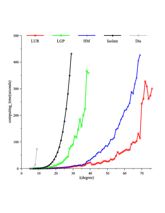
Figure 1: Timings for the system $\{f,g\}$ with simple roots, where $f(g)=randpoly([x,y],degree=i,coeffs=rand(-100..100),dense)$.

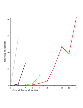
Figure 2: Timings for the system $\{f,g\}$ with multiple roots, where $p=randpoly([x,y,z],degree=ceil(i/2),coeffs=rand(-10..10),dense)$, $q=randpoly([x,y,z],degree=i-ceil(i/2),coeffs=rand(-10..10),dense)$ and $f$ is the square free part of ${\hbox{\rm{Res}}}_{z}(p,q)$, $g:=\frac{\partial f}{\partial y}$, where $ceil(t)$ is the minimal integer larger than a given real number $t$. The symbols for different solvers are the same as in Figure 1.

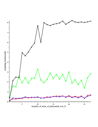
Figure 3: Timings for the system $\{f,g\}$ with simple roots, where $f(g)=randpoly([x,y],degree=15,terms=5i,coeffs=rand(-100..100),dense)$. The symbols for different solvers are the same as in Figure 1.

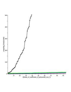
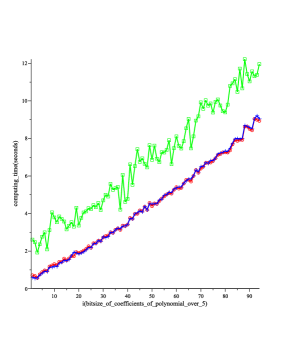
Figure 4: Timings for the system $\{f,g\}$ with simple roots, where $f(g)=randpoly([x,y],degree=15,coeffs=rand(-2^{5i}..2^{5i}),dense)$. The right one is the figure with large size without the timing for Isolate. The symbols for different solvers are the same as in Figure 1.

Figure 1 shows that LUR is the most efficient one among the five solvers. Then it is HM, LGP, Isolate and Dis in decreasing order. LUR stops for a system with degree 76 because the univariate polynomial equation solver outputs error since the equation is out of the ability of the univariate solver.

Figure 2 shows a comparison among different solvers for systems with multiple zeros. LUR is also the most efficient one among the five solvers. It works for the systems with multiple roots of degree $[49,48]$. Note that the bitsizes of the coefficients of the polynomials are larger than 100. That is why LUR seems slower comparing to itself in Figure 1. The solver HM becomes very slow for systems with multiple roots.

From Figures 3 and 4, we can find that LUR, LGP, HM almost stable for sparse systems. The reason is that all of them mainly involve resultant computation. Isolate is faster for sparse systems than for dense systems. The bitsizes of the polynomials influence all the solvers, especially for Isolate.

There is another efficient bivariate systems solver: Bisolve (Emeliyanenko et al., (2011)). It is implemented in C and use GPU parallel technique to deal with some symbolic computations such as resultant and gcd computations. In another paper related to Bisolve, the computing times running on the same machine and the same examples were improved a lot (Emeliyanenko et al., (2013)) compared to (Emeliyanenko et al., (2011)). It is around a half computing time compared to the old one. When comparing LUR and Bisolve, we use their new data in this paper. We do not compare with their implementation directly. But we compute the same examples taken from (Emeliyanenko et al., (2013)) on our machine. We compare the two methods in Table 1. Here, one part of data is taken from (Emeliyanenko et al., (2013)) directly. The other part of data is derived by running on our machine. Please see Table 1 for the details. We denote our machine as M2, theirs as M1 for convenience. We can find that LGP runs the same examples on M2 take around twice computing times (but a little less than ) as on M1 in the average level. In (Emeliyanenko et al., (2013)), they used some filtering techniques to validate a majority of the candidates early. BS means without filters, BS+all means with all filters enabled. For BS+all, there are two groups of data. One uses GPU, denoted as GPU-BS+all, the other does not, denoted as CPU-BS+all. BS in the table means BS using GPU, denoted as BS+GPU. For LUR, we list the times of computing the first resultant and isolating its real roots, denoted as $\mathrm{T}_{1}$ in Table 1. The total computing time is denoted as T.

Through we do not compare Bisolve with LUR directly, we compare them in an indirect way. The data in their paper shows that the filtering techniques improved the computing times a lot (usually more than one half) for Bisolve, especially for the systems with large bitsizes in coefficients. The parallel technique improved the Bisolve a lot (usually more than one half), but the improvement was not remarkable for systems with large bitsizes in coefficients. LGP is tested on both M1 and M2. The computing times of LGP on M1 are always around one half faster than on M2 for the same examples. We can find that LUR is usually faster than LGP, except for one or two examples. For some examples, LUR on M2 is faster than BS, CPU-BS+all on M1. The bitsizes of the coefficients of the systems influence BS and LUR deeper than GPU-BS+all and CPU-BS+all. We can find that for many examples, the total computing times of GPU-BS+all are less than the computing times for computing only the first resultant and its real root isolation. We use the computing times of GPU-BS+all and LGP to get a rate on M1, denoted as R1. Similarly, we can get R2 for LUR and LGP on M2. We can find that R1 is usually less than R2 except for some examples. The average level is around R1: R2 $\approx$ 1: 3. Note that the part of computing resultants, real root isolation and computing $s$ in LUR can be parallelized. Considering the influence of machines, parallel techniques and coding languages, our algorithm can be improved a lot.

From the comparisons before, we can conclude that LUR is efficient and stable for zero-dimensional bivariate polynomial systems.

comparing the computing times of Bisolve and LUR on special curves
Machine	Linux platform on a $2.8$ GHz					Win XP on Inter(R) Core(TM)
	$8$-Core Inter Xeon W$3530$					2 quad CPU Q9400 @2.66GHz
	with $8$MB of L$2$ cache					with 2$\times$3MB of L2 cache
Code language	C$++$				Maple
GPU speedup	YES			NO
curves	BS	BS$+$all	$\frac{\mathrm{BS+all}}{\mathrm{LGP}}$	BS$+$all	LGP	$\frac{\mathrm{LUR}}{\mathrm{LGP}}$	LGP	LUR
								$T_{1}$	$T$
13_sings_9	2.13	0.97	0.35	1.65	2.81	0.83	4.78	1.78	3.95
FTT_5_4_4	48.03	20.51	0.10	52.21	195.65	0.18	279.48	2.20	50.34
L4_circles	0.92	0.74	0.10	1.72	7.58	0.16	13.86	0.49	2.22
L6_circles	3.91	2.60	0.05	16.16	51.60	0.18	47.45	2.33	8.77
SA_2_4_eps	0.97	0.44	0.09	4.45	4.69	0.89	8.92	2.20	7.92
SA_4_4_eps	4.77	2.01	0.04	91.90	54.51	1.15	88.63	12.23	102.17
challenge_12	21.54	7.35	0.20	18.90	37.07	0.85	57.20	4.45	48.63
challenge_12_1	84.63	19.17	0.07	72.57	277.68	0.32	385.28	7.99	123.86
compact_surf	12.42	4.06	0.34	12.18	12.00	2.81	15.39	2.20	43.19
cov_sol_20	28.18	5.77	0.03	16.57	171.62	0.03	393.84	5.11	12.97
curve24	85.91	8.22	0.22	25.36	37.94	0.21	65.11	6.56	13.75
curve_issac	2.39	0.88	0.02	1.82	3.29	0.39	6.39	0.63	2.47
cusps_and_flexes	1.17	0.63	0.26	1.27	2.43	0.83	5.47	1.78	4.56
degree_7_surf	29.92	7.74	0.06	90.50	131.25	0.14	203.30	10.58	28.80
dfold_10_6	3.30	1.55	0.41	17.85	3.76	0.50	6.19	0.13	3.08
grid_deg_10	2.49	1.20	0.45	2.49	2.64	0.71	6.06	2.19	4.30
huge_cusp	9.64	6.44	0.06	13.67	116.67	0.41	224.98	76.00	91.28
mignotte_xy	timeout	243.16	-	310.13	timeout	-	timeout	322.00	325.08
spider	167.30	46.47	-	216.86	timeout	-	timeout	101.19	202.02
swinnerton_dyer	28.39	5.28	0.19	24.38	27.92	1.10	46.36	1.03	51.00
ten_circles	4.62	1.33	0.27	3.74	4.96	0.54	9.09	0.55	4.95
15, 10, dense	56.40	1.55	0.27	2.66	5.65	0.29	13.49	1.84	3.89
15, 128, dense	95.35	2.01	0.19	2.30	10.46	0.38	21.50	5.94	8.20
15, 512, dense	195.01	3.95	0.12	4.22	33.87	0.46	28.27	12.30	13.06
15, 2048, dense	timeout	19.89	0.10	20.45	190.86	0.45	233.13	100.58	105.58
15, 10, sparse	3.66	1.00	0.44	1.39	2.25	0.30	4.49	0.69	1.33
15, 128, sparse	12.14	1.25	0.29	1.35	4.27	0.38	8.83	2.73	3.36
15, 512, sparse	43.36	2.54	0.16	2.54	15.48	0.45	28.72	12.22	12.95
15, 2048, sparse	408.90	10.97	0.12	10.98	89.35	0.61	245.14	148.19	150.49

Table 1: Timings for multivariate case: the system are formed by random dense polynomials with the given degrees

Degree Type	LUR	Isolate	Dis
[3, 3, 3]	0.7644	0.0874	340.7092
[5, 5, 5]	27.1829	3.8826	-
[2, 9, 9]	10.1908	11.7686	-
[7, 7, 7]	614.1030	106.7302	-
[3, 15, 15]	498.4531	1720.2013	-

Table 2: Timings for multivariate case: the system are formed by random dense polynomials with the given degrees

We also compare LUR with other efficient solvers for multivariate polynomial systems. We compare mainly with Dis and Isolate, see Table 2. LUR is always faster than Dis. When there is a polynomial with lower degree in the system, LUR is faster than Isolate and it is slower than Isolate for the systems with equal degrees. The reason is that the former case can be projected to a bivariate system of lower degree. For the system with more variables, it is similar. Note that the core of Isolate is in C, ours is in Maple. For the same algorithm, the implementation in C is usually several times faster than Maple.

References

- Alonso et al., (1996) M. E. Alonso, E. Becker, M. F. Roy, and T. Wörmann. Zeros, multiplicities, and idempotents for zerodimensional systems. In Algorithms in Algebraic Geometry and Applicatiobns, pages 1–15. Birkhauser, 1996.
- Basu et al., (2003) S. Basu, R. Pollack, and M. F. Roy. Algorithms in Real Algebraic Geometry. Springer, Berlin, 2003.
- Becker and Wörmann, (1996) E. Becker and T. Wörmann. Radical computations of zero-dimensional ideals and real root counting. Mathematics and Computers in Simulation, 42(4-6): 561–569, November 1996.
- Busé et al., (2005) L. Busé, H. Khalil, B. Mourrain. Resultant-Based Methods for Plane Curves Intersection Problems. CASC 2005: 75-92, 2005.
- Canny, (1988) J. F. Canny. Some algebraic and geometric computation in pspace. In ACM Symp. on Theory of Computing, pages 460–469. SIGACT, 1988.
- Cheng et al., (2009) J. S. Cheng, X. S. Gao, J. Li. Root isolation for bivariate polynomial systems with local generic position method. ISSAC 2009: 103–110, 2009.
- Cheng et al., (2012) J. S. Cheng, X. S. Gao, and L. Guo. Root isolation of zero-dimensional polynomial systems with linear univariate representation. Journal of Symbolic Computation 47(7): 843–858, 2012.
- Cheng et al., (2009) J. S. Cheng, X. S. Gao, and C. K. Yap. Complete numerical isolation of real roots in zero-dimensional triangular systems. Journal of Symbolic Computation, 44(7): 768–785, July 2009.
- Corless et al., (1997) R. Corless, P. Gianni, and B. Trager. A reordered schur factorization method for zero-dimensional polynomial systems with multiple roots. ISSAC 1997: 133–140, 1997.
- Cox et al., (1998) D. A. Cox, J. B. Little and D. O’Shea. Using Algebraic Geometry, GTM, Volume 185, Springer, 1998.
- Diochnos et al., (2009) D. I. Diochnos, I. Z. Emiris, and E. P. Tsigaridas. On the asymptotic and practical complexity of solving bivariate systems over the reals. Journal Symbolic Computation, Special issue for ISSAC 2007, 44(7): 818-835, 2009.
- Emeliyanenko et al., (2011) P. Emeliyanenko, E. Berberich, M. Sagraloff. An Elimination Method for Solving Bivariate Polynomial Systems: Eliminating the Usual Drawbacks. In Algorithm Engineering and Experiments (ALENEX), 2011.
- Emeliyanenko et al., (2013) P. Emeliyanenko, A. Kobel, E. Berberich, M. Sagraloff. Exact Symbolic-Numeric Computation of Planar Algebraic Curves. to appear in Theoretical Computer Science (TCS), 2013.
- Emeliyanenko et al., (2012) P. Emeliyanenko, M. Sagraloff. On the Complexity of Solving a Bivariate Polynomial System. ISSAC2012: 154–161, 2012.
- Emiris et al., (2008) I. Z. Emiris, B. Mourrain, E. P. Tsigaridas. Real Algebraic Numbers: Complexity Analysis and Experimentation. Reliable Implementation of Real Number Algorithms, 57-82, 2008.
- Emiris and Tsigaridas, (2005) I. Z. Emiris, E. P. Tsigaridas: Real Solving of Bivariate Polynomial Systems. CASC 2005, 150-161, 2005.
- Fulton, (1984) W. Fulton. Introduction to Intersection Theory in Algebraic Geometry. Providence, R.I, Washington, DC, 1984.
- Giusti et al., (2001) M. Giusti, G. Lecerf, and B. Salvy, A Gröbner free alternative for polynomial system solving. Journal of Complexity, 17: 154-211, 2001.
- Gao and Chou, (1999) X. S. Gao and S. C. Chou. On the theory of resolvents and its applications. Sys. Sci. and Math. Sci., 12: 17–30, 1999.
- Giusti and Heintz, (1991) M. Giusti and J. Heintz. Algorithmes - disons rapides -pour la dècomposition d’une varièté algébrique en composantes irréducibles et équidimensionnelles. In Proc MEGA’ 90, pages 169–193. Birkhäuser, 1991.
- Hong et al., (2008) H. Hong, M. Shan, and Z. Zeng. Hybrid method for solving bivariate polynomial system. In SRATC 2008, 2008.
- Kerber and Sagraloff, (2012) M. Kerber, M. Sagraloff. A worst-case bound for the topology computation of algebraic curves. Journal of Symbolic Computation, 47, 239-258, 2012.
- Kobayashi et al., (1988) H. Kobayashi, S. Moritsugu, and R. W. Hogan. Solving systems of algebraic equations. In ISSAC 1988: 139–149, 1988.
- Mantzaflaris et al., (2011) A. Mantzaflaris, B. Mourrain, E. P. Tsigaridas. On continued fraction expansion of real roots of polynomial systems, complexity and condition numbers. Theor. Comput. Sci. 412(22): 2312–2330, 2011.
- Mignotte, (1992) M. Mignotte. Mathematics for Computer Algebra, Springer-Verlag, 1992.
- Moore et al., (2009) Ramon E. Moore, R. Baker Kearfott, Michael J. Cloud, Introduction to Interval Analysis, Society for Industrial and Applied Mathematics, Philadelphia, 2009.
- Mourrain and Pavone, (2009) B. Mourrain, J.-P. Pavone, Subdivision methods for solving polynomial equations Journal of Symbolic Computation, 44 (3): 292–306, 2009.
- Pan, (2000) V. Y. Pan. Approximating complex polynomial zeros: modified Weyl’s quadtree construction and improved Newton’s iteration. J. of Complexity, 16(1): 213–264, 2000.
- Pan, (2002) V. Y. Pan. Univariate Polynomials: Nearly Optimal Algorithms for Numerical Factorization and Root-finding. Journal Symbolic Computation 33(5): 701-733, 2002.
- Pan and Tsigaridas, (2013) V. Y. Pan and E. P. Tsigaridas: On the boolean complexity of real root refinement. ISSAC 2013: 299–306, 2013
- Qin et al., (2012) X. Qin, Y. Feng, J. Chen, J. Zhang. Parallel computation of real solving bivariate polynomial systems by zero-matching method. Applied Mathematics and Computation, to appear, 2012.
- Reischert, (1997) D. Reischert. Asymptotically fast computation of resultants. Proceedings of ISSAC 97, Hawaii. pp. 233 C240. ACM Press, 1997.
- Rouillier, (1999) F. Rouillier. Solving zero-dimensional systems through the rational univariate representation. Applicable Algebra in Engineering, Communication and Computing, 9(5): 433–461, May 1999.
- Rouillier and Zimmermann, (2003) F. Rouillier and P. Zimmermann. Efficient isolation of polynomial real roots. J. of Comp. and App. Math., 162(1): 33-50, 2003.
- Sagraloff, (2012) M. Sagraloff. When Newton meets Descartes: A Simple and Fast Algorithm to Isolate the Real Roots of a Polynomial, ISSAC2012: 297–304, 2012.
- Schönhage, (1982) A. Schönhage. The fundamental theorem of algebra in terms of computational complexity. Manuscript. Univ. of Tübingen, Germany, 1982. URL: http://www.iai.uni-bonn.de/ schoe/fdthmrep.ps.gz.
- Stahl, (1995) V. Stahl. Interval methods for bounding the range of polynomials and solving systems of nonlinear equations, PhD Thesis, Johannes Kepler University, Austria, 1995.
- Tan and Zhang, (2009) C. Tan and S.C. Zhang. Separating element computation for the rational univariate representation with short coefficients in zero-dimensional algebraic varieties. Journal of Jilin University (Science Edition), 47: 174–178, 2009.
- Xia and Yang, (2002) B. Xia and L. Yang. An algorithm for isolating the real solutions of semi-algebraic systems. Journal of Symbolic Computation, 34(5): 461–477, 2002.
- Yap, (2000) C. Yap. Fundamental Problems of Algorithmic Algebra, Oxford University Press, New York, 2000.
- Yokoyama et al., (1989) K. Yokoyama, M. Noro, and T. Takeshima. Computing primitive elements of extension fields. Journal of Symbolic Computation, 8(6): 553–580, 1989.