Objective Identification of Informative Wavelength Regions in Galaxy Spectra

Abstract

Understanding the diversity in spectra is the key to determining the physical parameters of galaxies. The optical spectra of galaxies are highly convoluted with continuum and lines which are potentially sensitive to different physical parameters. Defining the wavelength regions of interest is therefore an important question. In this work, we identify informative wavelength regions in a single-burst stellar populations model by using the CUR Matrix Decomposition. Simulating the Lick/IDS  spectrograph configuration, we recover the widely used $\mathrm{D}_{n}(4000)$, H$\beta$ and $\mathrm{H}{\delta_{A}}$  to be most informative. Simulating the SDSS spectrograph configuration with a wavelength range 3450–8350 Å and a model-limited spectral resolution of 3 Å, the most informative regions are: first region–the 4000 Å break and the H$\delta$ line; second region–the Fe-like indices; third region–the H$\beta$ line; fourth region–the G band and the H$\gamma$ line. A Principal Component Analysis on the first region shows that the first eigenspectrum tells primarily the stellar age, the second eigenspectrum is related to the age-metallicity degeneracy, and the third eigenspectrum shows an anti-correlation between the strengths of the Balmer and the Ca K & H absorptions. The regions can be used to determine the stellar age and metallicity in early-type galaxies which have solar abundance ratios, no dust, and a single-burst star formation history. The region identification method can be applied to any set of spectra of the user’s interest, so that we eliminate the need for a common, fixed-resolution index system. We discuss future directions in extending the current analysis to late-type galaxies.

1 Introduction

It has long been known that the diversity in spectra of galaxies is driven by the variance in their underlying physical properties, such as stellar age and metallicity. The line indices, or the relatively narrow regions of a spectrum, are isolated for the parameter sensitivities. Faber (1973) found that metallicity-sensitive indices from a 10-filter photometric system correlate with the luminosity of ellipticals, giving incredible insights to the role of gravitational potential well to the chemical evolution in those galaxies. The concept of “informative” wavelength regions had since been extended to spectroscopy. Perhaps the most well-known example is the 4000 Å break (Bruzual A., 1983) and its correlation with the stellar age and metallicity in early-type galaxies. Worthey et al. (1994) later assembled 21 absorption indices and measured them for several hundred stars in the Galaxy, and the same set were measured by Trager et al. (1998) for several hundred globular clusters and galaxies. They are called the Lick/IDS  indices (Burstein et al., 1984; Faber et al., 1985). These indices are continuum subtracted, where the continua are defined on the left and right flanks in the vicinity of the actual index wavelength range. Within an index wavelength range, one or more absorption lines, or a feature, are present. Therefore, the index strength can be a sensitive measure for specific galaxy parameters. The $\mathrm{D}_{n}(4000)$(Balogh et al., 1999) and $\mathrm{H}{\delta_{A}}$ (Worthey & Ottaviani, 1997) indices were subsequently defined, and were used to constrain stellar age and the starburst mass fraction in galaxies (Kauffmann et al., 2003).

The concept of informative wavelength regions has also been used in conjunction with a popular data compression technique, the Principal Component Analysis (PCA), to derive physical parameters of galaxies. Each spectrum in a galaxy sample is represented by the weighted sum of the same orthogonal basis, hereafter the eigenspectra (Connolly et al., 1995), and the weights are called the eigencoefficients. The lowest orders of the eigenspectra encapsulate most of the sample variance in nearby galaxies (Yip et al., 2004), forming a subspace which lies in a higher-dimensional wavelength space. Using PCA, Wild et al. (2007) have measured, for a galaxy sample from the SDSS (York et al., 2000), the eigencoefficients within the restframe 3750–4150 Å out of the full optical wavelength range available, 3800–9200 Å  in the observed frame. The eigencoefficients were used to correlate with physical properties of the galaxies. Later, Chen et al. (2012) have estimated model-based stellar populations and dust parameters for a sample of SDSS galaxies. They used eigencoefficients calculated in the 3700–5500 Å range, in conjunction with the Bayesian parameter estimation method.

Despite decades of effort and progress, the Lick/IDS indices remain to be subjective. The root cause lies in the difficulties in defining the true continua in the vicinity of a feature. Two main hurdles are: (1) There is no “true” continuum in late-type stars at the Lick/IDS  spectral resolution and the continua are “pseudo” (Worthey et al., 1994). (2) The location and the width of the pseudocontinua are subjective. The location are chosen to flank the feature, and the width to be large enough in order to minimize the effect of typical stellar velocity dispersion of galaxies on the measured index strengths (Worthey et al., 1994; Trager et al., 1998). For a galaxy of a given velocity dispersion, these characteristics determine the absorption lines present within the pseudocontinua, in turn impact the parameter sensitivity of the corresponding feature. For example, Jones & Worthey (1995) found in a single-burst stellar populations model that the narrow Balmer index, H$\gamma$_HR, is significantly more sensitive to stellar age than its broad counterpart, $\mathrm{H}{\gamma_{A}}$, suggesting that the broader Balmer indices may be contaminated by metal lines. They are the Fe I lines (Thomas et al., 2004), present in the pseudocontinua of the broad, higher-order Balmer indices (Worthey & Ottaviani, 1997).

The PCA approach (Wild et al., 2007; Chen et al., 2012) abandoned the use of pseudocontinua and bypassed difficulties (1) & (2), but the feature wavelength ranges were chosen subjectively to include the 4000 Å break, unlike the Lick/IDS index system in which they were measured. Like the case in pseudocontinua, the identity and the width of a feature can impact its parameter sensitivity, because they determine what absorption lines are present within. The reason for using PCA  is that the eigenspectra are orthogonal, so that each eigenspectrum is potentially sensitive to individual physical parameters. Clearly, the next-generation approach is to combine the orthogonal-decomposition strength of PCA  with objectivity in defining the feature wavelength regions.

The main goals of this paper are to identify the informative wavelength regions in an objective manner, and to associate physical significance with them. The analyses are performed on a solar-abundance model of Simple Stellar Populations that is defined by two parameters, stellar age and metallicity. We use the CUR Matrix Decomposition  (Drineas et al., 2008; Mahoney & Drineas, 2009), a powerful machine learning technique which has the ability to select statistically informative columns from a data matrix. The key characteristics of our approach are: (a) The continua are not explicitly used in the region identification, bypassing the above-mentioned (1) & (2) which plague the Lick/IDS indices. (b) Different from the previous PCA  approach (Wild et al., 2007; Chen et al., 2012), in this work the regions are determined objectively, in terms of both the identity and the width.

We cast an eye towards estimating physical parameters of real galaxies. This work results in two related applications. First, the identified regions and the parameter-eigencoefficient relation can be used to determine the stellar age and metallicity of those early-type galaxies which have solar abundance ratios, no dust, and a single-burst star formation history. Second, our region identification method can be applied to any set of model spectra. Users can generate their own parameter-eigencoefficient  relation from the model, and use that to estimate parameters of galaxies from the observed spectra. Therefore, the intricate processes (Worthey & Ottaviani, 1997) involved in conforming to a common index system, which attempt to account for the difference in spectral resolution between the observed spectra and the system, can be eliminated.

In §2, we present the model spectra. In §3, we present the CUR Matrix Decomposition and describe how it is used to identify informative wavelength regions in the model spectra. In §4, we present the identified regions, the comparison to the existing line indices, and their physical significance. In §5, we conclude our work and discuss next steps. Vacuum wavelengths are used throughout the paper.

2 Model & Preprocessing

We wish to derive a set of informative regions applicable for estimating the stellar age and metallicity in galaxies which have no dust and follow a single-burst star formation history. Hence we perform the CUR Matrix Decomposition  on a model with known physical parameters. The Bruzual & Charlot (2003) stellar populations model is used. For a chosen stellar initial mass function (IMF) and stellar isochrones, the model provides spectra of Simple Stellar Populations (SSPs) spanning 6 stellar metallicities by mass ($Z$ = 0.0001, 0.0004, 0.004, 0.008, 0.02, 0.05) and 221 stellar ages (0 – 20 Gyr, distributed roughly in equally-sized logarithmic bins). We adopt the Chabrier (2003) IMF and Padova 1994 isochrones (Girardi et al., 1996, and references therein), and these choices are not expected to impact our results qualitatively. We do not add extinction to our model. And, there is no stellar velocity dispersion variance in our model, in contrast to the galaxy spectra used the Lick/IDS  indices measurement (Trager et al., 1998). We choose not to study the effect of noise and other artifacts on the identified regions, because other approaches (e.g., Robust PCA  by Budavári et al., 2009) can be used to derive robust eigenspectra and eigencoefficients (Dobos et al., 2012) for regions in real galaxy spectra. The Bruzual & Charlot (2003) model has solar abundance ratios, which may limit the application of our regions from many early-type galaxies (e.g., Worthey et al., 1992) having non-solar values. We decide to identify a new set of regions when a more sophisciated stellar populations model is available in the future.

A preprocessing is carried out to ensure that (i) each and every spectrum is unique, (ii) all of the flux values are available (i.e., no NaN, and no zero vector), and (iii) the final ages and metallicities are selected as such they follow a rectangular parameter grid. This step results in the same 6  metallicities but 182 ages (2.5 Myr – 20 Gyr), or 1092 SSP spectra in total.

The SSP are rebinned, in a flux-conserving fashion, to two configurations: the Lick/IDS and the SDSS. The Lick/IDS configuration allows us to compare the identified regions to the widely used indices in the literature. On the other hand, the SDSS configuration will result in regions with a spectral resolution higher than the Lick/IDS  indices and closer to the SDSS galaxy spectra. The Lick/IDS  configuration is a wavelength range 3800–6400 Å, a spectral resolution of 9 Å FWHM, and a sampling of 1.25 Å per pixel. The model spectra are therefore scaled down in resolution by convolving with a Gaussian function. The function has a FWHM equal to the Bruzual & Charlot (2003) resolution (3 Å FWHM  within the optical) quadrature-subtracted from the targeted resolution. This choice is made to mimic the Lick/IDS  spectrograph configuration (4000–6400 Å in air wavelengths, Burstein et al., 1984) as well as to include both the left and the right flanks of $\mathrm{D}_{n}(4000)$. They are referred as the $\mathrm{D}_{n}(4000)$L and $\mathrm{D}_{n}(4000)$R for convenience. The SDSS configuration is a wavelength range 3450–8350 Å, a spectral resolution of 3 Å FWHM, and a sampling of 69 km s^-1 per pixel. The choice of 3 Å is limited by the instrumental resolution of the Bruzual & Charlot (2003) model. The actual spectral resolution in the SDSS is 1800 (corresponds to 166 km s^-1), higher than that of the model at the shortest wavelengths, and is 1.9 Å at $\lambda=$ 3450 Å. The wavelength range is tuned to coincide with the restframe wavelength range of spectra in most nearby SDSS galaxies, for which the median redshift is 0.1. The observed-frame wavelengths of the SDSS spectrograph are ranged from 3800–9200 Å.

The spectra are converted from flux density (in erg s^-1 Å^-1) to flux (in erg s^-1) using $f_{\lambda}^{\prime}=f_{\lambda}\cdot\Delta{\lambda}$. The data values, which will be cast into a matrix later, are in the flux unit. The mean spectrum of the model is subtracted from each SSP  spectrum. The data cloud formed by the spectra are hence centered in the wavelength space. The spectra are not continuum subtracted, as such no assumption on the true continuum is made.

2.1 Extended Lick/IDS indices

We assemble the 21  Lick/IDS  indices from Trager et al. (1998, their whole Table 2), the 4 indices from Worthey & Ottaviani (1997, $\mathrm{H}{\delta_{A}}$, $\mathrm{H}{\gamma_{A}}$, $\mathrm{H}{\delta_{F}}$, $\mathrm{H}{\gamma_{F}}$  or their whole Table 1) and the 1 index from Balogh et al. (1999, $\mathrm{D}_{n}(4000)$ in Table 1), and name the 26  collectively as “the Extended Lick/IDS indices” for convenience. The details are listed Table 1.

3 Analysis

3.1 CUR Matrix Decomposition

The CUR Matrix Decomposition  (Drineas et al., 2008; Mahoney & Drineas, 2009) is a novel method that has been used for large-scale data analysis in multiple disciplines. The main idea is to approximate a potentially huge data matrix with a lower rank matrix, where the latter is made with a small number of actual rows and/or columns of the original data matrix. The selected rows and columns are therefore statistically informative. The data in this work are model spectra, selecting the rows and columns corresponds to selecting the spectrum IDs and wavelengths, respectively. We will use only the column part of the decomposition, selecting informative wavelengths in the spectra. Further details of the CUR Matrix Decomposition  are presented in Appendix A.

We start by constructing a $m\times n$ data matrix $A$, where each row is a single SSP spectrum from the model spectra. That is, $A_{ij}=f^{i}_{\lambda_{j}}\cdot\Delta{\lambda_{j}}$ is the flux of the $i$th spectrum at the $j$th wavelength. The full set of model spectra (§2) is used, so that the sample variance in the matrix is driven by both stellar age and metallicity. A Singular Value Decomposition (SVD) is performed on $A$

$$A=U\,\Sigma\,V^{T}\ ,$$ (1)

which gives $U$ and $V$, the orthonormal matrices in which the columns are respectively the left and right singular vectors; and $\Sigma$, the diagonal matrix containing the singular values. For a chosen $k$, the LeverageScore at a given wavelength is

$$p_{\lambda}=\frac{\sum_{j=1}^{\mathit{k}}\,\left(v^{j}_{\lambda}\right)^{2}}{k}\ ,$$ (2)

where $v^{j}_{\lambda}$ is the $j$th right singular vector. The collection of the $k$ right singular vectors forms an orthonormal basis to the fluxes in the high-dimensional wavelength space. The larger the $v^{j}_{\lambda}$ value, the larger the sample variance is projected from the $j$th basis vector onto the given wavelength axis. The $p_{\lambda}$ is hence proportional to the total projected sample variance from altogether $k$ basis vectors onto that wavelength axis. In other words, $p_{\lambda}$ measures the information contained in a wavelength. This information tells the sample variance driven by the physical parameters, stellar age and metallicity.

The ordering of the spectra per row in the matrix $A$ does not impact the ordering of the right singular vectors. As long as the same set of spectra is used, and the same $k$ is chosen, the same $p_{\lambda}$ will result. The $k$ values will be chosen in an objective manner in this work.

3.2 Region Identification Procedure

The two main steps in the region identification are to select the informative wavelength, $\lambda_{I}$, and to determine its region of influence, ROI. To select $\lambda_{I}$, we pick from the available wavelengths the one with the highest $p_{\lambda}$. To determine the ROI, we observe several guidelines: (A) A region  is contiguous in wavelength. (B) A region  is allowed to be asymmetric about $\lambda_{I}$. (C) Regions can overlap with each other. (D) We expect that, if a region can indeed be defined, the $p_{\lambda}$  would decline to zero when approaching the left and right wavelength bounds, because the fluxes Combining the above considerations, a ROI is calculated as follows. Starting at the wavelength that is selected ($\lambda_{I}$), we attempt to include a pixel to its immediate left or right. The accumulated $p_{\lambda}$ of both scenarios are calculated, called $p^{S}_{\lambda}$. The pixel gives the higher $p^{S}_{\lambda}$ is added to the region. The procedure is repeated until the last ($i$th) pixel is included, as such the following convergence criterion is satisfied

$$\left|\frac{{p^{S}_{\lambda}}_{i}-{p^{S}_{\lambda}}_{i-1}}{\lambda_{i}-\lambda_{i-1}}\right|\leq T\cdot\frac{\sum_{\lambda=\lambda_{1}}^{\lambda_{N}}p_{\lambda}}{\lambda_{N}-\lambda_{1}}=T\cdot\frac{1}{\lambda_{N}-\lambda_{1}}\ .$$ (3)

That is, the change of the information content of a region per unit wavelength is a constant. We tie the constant to the average information expected in the case where every wavelength is equally informative. The threshold, $T$, is set to be 0.7  in this work. This value is not unity, consistent with the fact that the $p_{\lambda}$  are not uniform. More importantly, this choice enables us to obtain converged NaD-region  width (§4) for both the Lick/IDS  and the SDSS configurations (Figure 3 and Figure 6, respectively). The atomic lines, such as NaD, have well-defined central wavelengths and widths. They are therefore good standards for checking various identification approaches. For $T$= 0.7 $\pm$ 0.1 also give the width convergence in the SDSS configuration. The generality of this convergence for arbitrary spectra is however not yet established.

A ROI is fully indicated by the left and right wavelength bounds [$\lambda_{S},\lambda_{E}$]. Once the $\lambda_{I}$ and the [$\lambda_{S},\lambda_{E}$] are determined, they are labeled as a “Region” and all of the involved pixels are masked out in the next $\lambda_{I}$  and ROI  selection. The process is repeated until either no more pixels are available, or the desired number of regions is reached. We then use

$$\mathrm{\textit{LeverageScoreSum}}=p^{S}=\sum_{\lambda=\lambda_{S}}^{\lambda_{E}}p_{\lambda}$$ (4)

as the measure for the information contained in a region.

3.3 Relation of CUR to PCA

PCA has become a standard technique in spectral analyses. In extragalactic studies, it has been applied to remove sky from galaxy spectra (Wild & Hewett, 2005), to understand the diversity in galaxies (e.g., Connolly et al., 1995; Yip et al., 2004; Dobos et al., 2012) and quasars (e.g., Francis et al., 1992; Shang et al., 2003; Yip et al., 2004), to separate host galaxy contribution from broadline AGN spectra (Vanden Berk et al., 2006), and to find supernovae in large galaxy spectral samples (Madgwick et al., 2003; Krughoff et al., 2011), and many more studies. These works used the fact that PCA compresses the data in the object space, leaving the number of wavelength bins in each eigenspectrum unchanged from that of the input spectra. The CUR Matrix Decomposition provides us a new way to compress the data, so that even the variable space can be compressed. The variable in the current context is the wavelength.

3.4 Spectrum Cutout Analysis

The next step is to compare the regions quantitatively. We prepare spectral segments of each region  that are cut out from the model spectra. The set of cutouts of each region form a column subspace (in $\mathbb{R}^{m}$) of the original $m\times n$ data matrix $A$ (e.g., Strang, 1988). The number of cutout pixels is less than the number of spectra in this work. Therefore, the rank of the subspace, at maximum, is equal to the number of pixels of that region. Its actual value would depend on the dimension of the subspace in question. Three subspace measures are used: (I) the cosine of the angle between two subspaces as defined by Gunawan, Neswan, & Setya-Budhi (2005), $\cos\theta_{\mathrm{GNS}}$. (II) The dot product between the first left-singular vectors of the two subspaces, $\cos\theta_{\mathrm{PC1}}$. (III) The Pearson correlation coefficient between the integrated fluxes of the two regions, $r$.

The subspace measure (I) is calculated as follows. For the $i$th region  with number of wavelength bins equal to $n^{(i)}$, we cut out from the original data matrix $A$ the corresponding submatrix $A^{(i)}$, size $m\times n^{(i)}$. A SVD is performed on the submatrix, $A^{(i)}=U^{(i)}\Sigma^{(i)}{V^{T}}^{(i)}$. The angle between the $i$th and the $j$th regions, with $1\leq n^{(i)}\leq n^{(j)}$, is calculated by applying the formula in Gunawan, Neswan, & Setya-Budhi (2005)

$$\cos\theta_{\mathrm{GNS}}=\sqrt{det(M^{T}M)}\ ,$$ (5)

where we put the matrix $M={U^{(j)}}^{T}{U^{(i)}}$. The symbol $det$ denotes the determinant, and $T$ the transpose, of a matrix. They have shown that $\cos\theta_{\mathrm{GNS}}$  is proportional to the volume of the parallelepiped spanned by the projection of the basis vectors of the lower-dimensional subspace on the higher-dimensional subspace. The one dimensional (1D) case is helpful for us to grasp the picture: the matrix product $M^{T}M$ becomes the dot product between the two 1D basis vectors.

From the SVD of the regions we can also calculate the dot product between the first left-singular vectors of any two regions, i.e., the subspace measure (II). Indeed, any order of singular vector can be considered, but we pick the first vector because it captures the maximum sample variance.

3.5 Parameter Sensitivity of Regions

To associate physical significance with the regions, we explore the correlation between a chosen parameterization of a region and the physical parameters defining the model. We start by examining the Pearson correlation coefficient formula, the correlation between two variables $X$ and $Y$ (each has $m$ components, $m$ being the number of spectra/objects) is equivalent to the dot product between two vectors in the object space  (each vector has $m$ components). We hereafter use “the correlation between two subspaces (in the variable space)” and “the angle between two subspaces (in the object space)” interchangeably.

This rather simple observation is highly instrumental for quantifying the parameter sensitivity of a region. If the subspace formed by a region is correlated with a parameter, then the two vectors – one is a chosen parameterization of the subspace, and another is the parameter itself (vector $p$), both have $m$ components – should be parallel to each other in the object space. The vector $p$ is either stellar age or metallicity. The angle between the two vectors can be represented by their dot product. We pick two parameterizations for a region, namely, the first and the second left-singular vectors (vectors $u^{1}$  and $u^{2}$), as most of the information is encapsulated by the lowest-order modes.

4 Results

4.1 Informative Regions: Lick/IDS Configuration

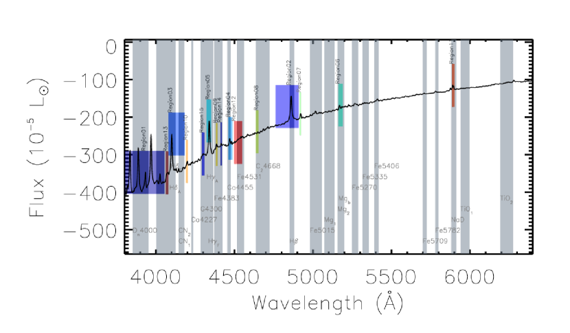
Figure 2: The first 15  informative wavelength regions, identified for wavelengths 3800–6400 Å  at 9 Å  spectral resolution, or the Lick/IDS configuration. The gray bars illustrate the Extended Lick/IDS indices. The first three regions comprises 4000 Å break, H$\beta$ and H$\delta$. The wavelengths in the vicinity of 5500 Å are not selected, in qualitative agreement with the Extended Lick/IDS indices. The background is one of the mean-subtracted spectra in the model. The bottom of a region label marks the $\lambda_{I}$ of that region.

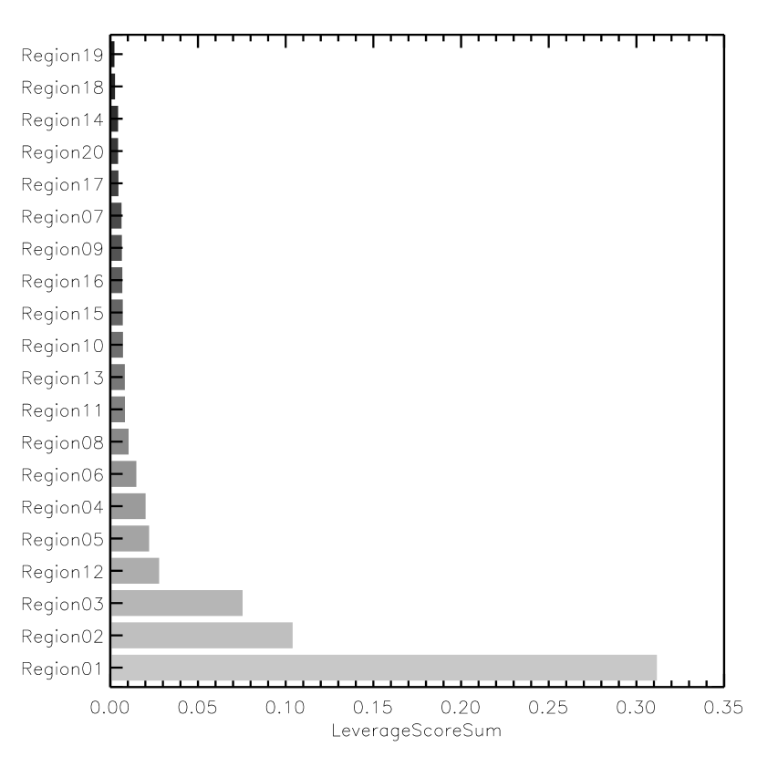
Figure 4: The LeverageScoreSum of the identified regions in the Lick/IDS  configuration, sorted by the amplitude. The first three regions are most informative.

The identified wavelength regions using our approach are shown in Figure 2. The corresponding $\lambda_{I}$, $\lambda_{S},\lambda_{E}$, as well as the overlapping Extended Lick/IDS indices, are given in Table 2. From the width convergence of Na D-region (Figure 4), $k$ is set to be 10. The following regions are found, in the order of importance:

• 1st: Comprises the 4000 Å break. The LeverageScoreSum  is a factor of a few or more larger than those of the other regions.

• 2nd: Comprises the H$\beta$ line.

• 3rd: Comprises the H$\delta$ line. The LeverageScoreSum  is comparable to that of the H$\beta$-region.

• 4th: Comprises the Fe4531, which belongs to the “Fe-like indices” family (Trager et al., 1998).

• 5th: Comprises the G band. The G band is primarily arisen from CH molecules and their energy levels are therefore many. Not too surprisingly, it is blended with H$\gamma$ to form a single region. The G band and the H$\gamma$ indices are also not disjoint in wavelength in the Extended Lick/IDS indices definition (Table 1).

• Higher orders: Certain Extended Lick/IDS indices  are recovered in the higher-order regions.

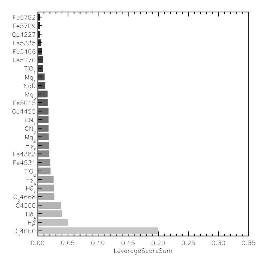
Figure 5: The LeverageScoreSum  of the Extended Lick/IDS indices, sorted by the amplitude. We note that there was no importance ordering in the Extended Lick/IDS indices originally. The indices $\mathrm{D}_{n}(4000)$, H$\beta$ and $\mathrm{H}{\delta_{A}}$ are found to be most informative.

The LeverageScoreSum  of our indices are plotted in Figure 4. The first three  regions are most informative. As a comparison, we also calculate the LeverageScoreSum  of the Extended Lick/IDS indices, shown in Figure 5. There was no importance ordering in the Extended Lick/IDS indices originally but they are sorted here nonetheless. The widely used indices, $\mathrm{D}_{n}(4000)$, H$\beta$ and $\mathrm{H}{\delta_{A}}$, are found indeed to be most informative.

We also see that the wavelengths in the vicinity of 5500 Å  are not selected, in qualitative agreement with the Extended Lick/IDS indices  (Figure 2). The wavelengths may be insensitive to stellar age nor stellar metallicity.

4.2 Informative Regions: SDSS Configuration

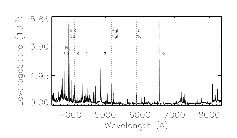
Figure 7: The LeverageScore  measures the information contained in a wavelength of a set of spectra. In the SDSS configuration. Some absorption lines are marked.

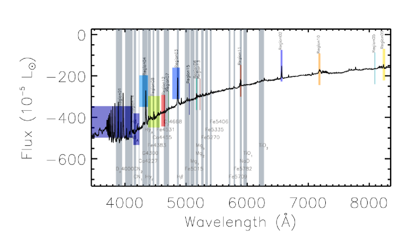
Figure 8: The first 15 informative wavelength regions identified for the wavelength range of 3450–8350 Å at a spectral resolution of 3 Å, or the SDSS configuration. The gray bars illustrate the Extended Lick/IDS indices. Similar to the Lick/IDS configuration, the 4000 Å break and the H$\delta$ line is found to be most informative; followed by the Fe-like indices; the H$\beta$ line; the G band and the H$\gamma$ line. The background is one of the mean-subtracted spectra in the model.

To identify informative regions in the SDSS configuration, the first step is to determine the appropriate $k$ value. Because of the higher resolution, the rank of the data matrix $A$ can be larger than the Lick/IDS case and the appropriate $k$ value can be different. Examine again the Na D-region width as a function of $k$  (Figure 6), it converges to 14.9 Å  with increasing $k$. We use $k$ = 25  in the region  identification. The LeverageScore  as a function of wavelength is plotted in Figure 7, with high amplitude seen in some absorption lines, and in the vicinity of the 4000 Å break. The most informative regions are plotted in Figure 8. They are, in the order of importance:

• 1st: Comprises the 4000 Å break and the H$\delta$ line. In the Extended Lick/IDS indices, as we noted earlier, the $\mathrm{D}_{n}(4000)$R and $\mathrm{H}{\delta_{A}}$ overlap in wavelength. So it is not entirely surprising that they form a single region. For example, there are likely many metal lines present in-between the $\mathrm{D}_{n}(4000)$L and $\mathrm{D}_{n}(4000)$R, so that the $\mathrm{D}_{n}(4000)$L, $\mathrm{D}_{n}(4000)$R and the H$\delta$ form one single region.

• 2nd: Comprises the Fe-like indices (Trager et al., 1998). This region appears to be more sensitive to stellar metallicity than the most informative region (the 4000 Å break and the H$\delta$ line), concluded from the dot product between the 2nd left-singular and stellar metallicity vectors (the last column of Table 3). Unfortunately, the LeverageScoreSum is a factor of 6 smaller, meaning this region is less informative. We have yet connected the two different quantities – the LeverageScoreSum and the dot product – to form a single measure for parameter sensitivity, which is beyond the scope of this work.

• 3rd: Comprises the H$\beta$ line.

• 4th: Comprises the G band and the H$\gamma$ line. The LeverageScoreSum amplitudes are comparable in the 2nd, 3rd, 4th most informative regions, about 0.05.

• Higher orders: The 7th most informative region comprises the H$\alpha$ (Table 4), which is detectable in most SDSS galaxies but falls outside of the Lick/IDS spectrograph wavelength range.

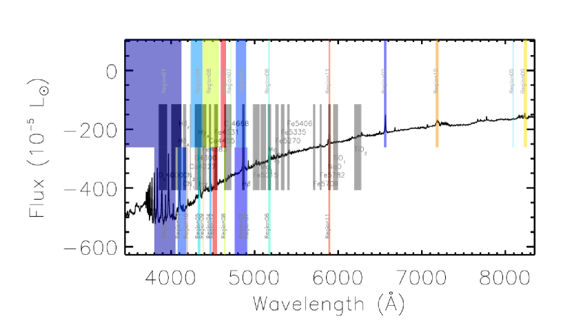
Figure 9: Comparison of the first 12  informative regions that are identified in the Lick/IDS (bottom) and SDSS (top) configurations. The gray bars show the Extended Lick/IDS indices.

The comparison of the regions between the Lick/IDS and the SDSS configurations is illustrated in Figure 9. For both sets, the 4000 Å break, H$\beta$, and H$\delta$ regions are among the top three most informative. We however expect the identified regions to depend on the spectral resolution and the wavelength coverage. To demonstrate the wavelength-coverage dependence, an extra region identification is carried out where we use the Lick/IDS spectral resolution and pixel size but the SDSS wavelength coverage (not shown). While the 4000 Å break remains to be the most informative region identified, its ROI is diffferent from that obtained in the Lick/IDS configuration, and is more similar to that obtained in the SDSS configuration. One possibility is that the true ROI of the 4000 Å break exceeds the shortest wavelength of the Lick/IDS configuration.

The dependence of the regions on the spectral resolution is difficult to be quantified generally. When the resolution is low, blended features cannot be resolved. The identified region can become broader than the true wavelength bound, where the latter may be identifiable only in higher-resolution spectra. When the resolution is high, the identified regions may not be optimal in terms of studying lower-resolution spectra, or they may not be the state-of-the-art for future surveys. To avoid these complicated situations, it is desirable to treat the identification method, instead of the identified regions, to be general. As such, the method can be applied to any set of spectra of the user’s interest.

4.3 Relation Among Regions

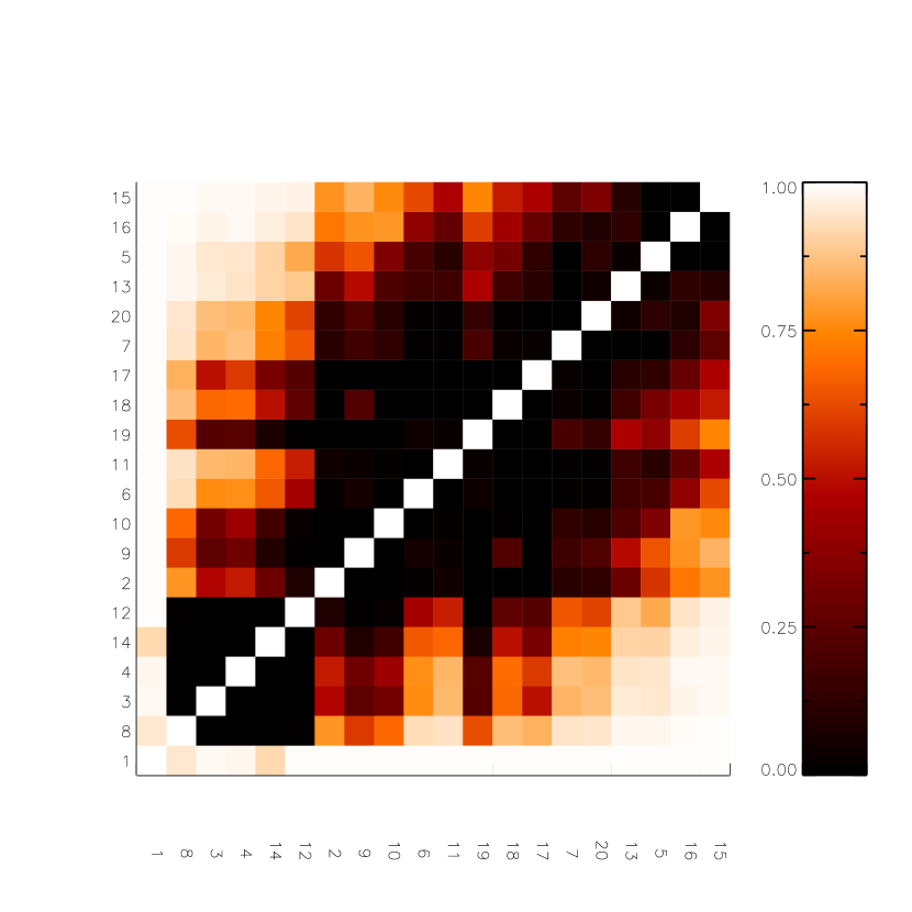
Figure 10: The $\cos^{2}\theta_{\mathrm{GNS}}$  between the subspaces spanned by the spectrum cutouts of our identified regions, in the SDSS configuration. The line indices are sorted by their LeverageScoreSum. All regions are almost parallel to the Region01.

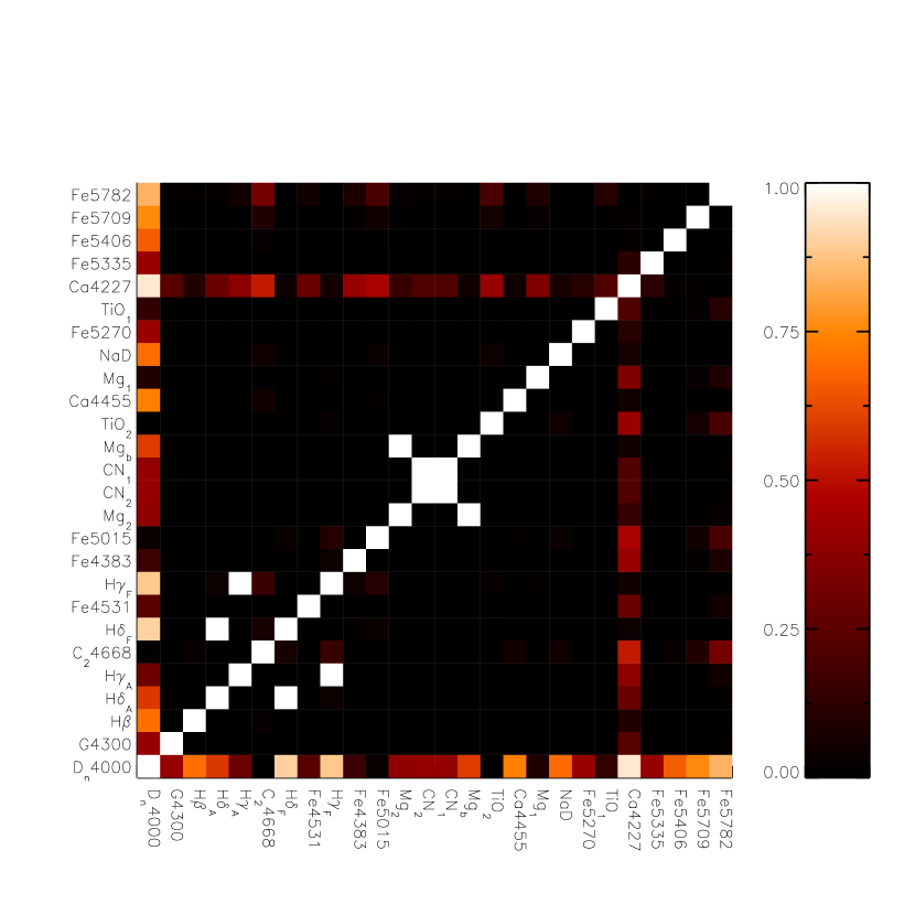
Figure 11: The $\cos^{2}\theta_{\mathrm{GNS}}$  between the subspaces spanned by the spectrum cutouts of the Extended Lick/IDS indices, in the SDSS configuration. The line indices are sorted by their LeverageScoreSum. Compared with the regions in Figure 10, we found fewer indices to be parallel to the 4000 Å break. There is also a marked difference in the number of orthogonal index pairs.

The angle between the subspaces spanned by any two regions is shown in Figure 10, in $\cos^{2}\theta_{\mathrm{GNS}}$  (Gunawan, Neswan, & Setya-Budhi, 2005). Those for the Extended Lick/IDS indices are shown in Figure 11. All of the higher-order regions are correlated with the first region, suggesting that the higher-order regions are not substantially different. This is not surprising considering the SSPs are defined by two parameters only, namely the stellar age and metallicity, and that the 4000 Å break is sensitive to both parameters. Some of the Extended Lick/IDS indices are also correlated with the $\mathrm{D}_{n}(4000)$  index, but not as many as in the Region01, nor as high the correlation amplitudes. This result shows that Region01  is more “complete” than the $\mathrm{D}_{n}(4000)$, in the sense that the corresponding subspace encapsulates most of the data directions.

The other pronounced difference between the Extended Lick/IDS indices  and the regions is that, in the former, there are many more cases where two indices are orthogonal. The region representation is therefore more “compact”, in the sense that we need fewer regions to encapsulate the various data directions.

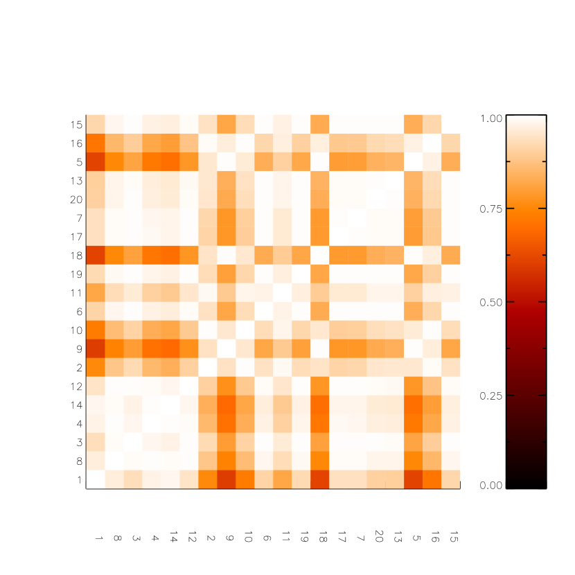
Figure 12: (Left) The squared Pearson correlation coefficient ($r^{2}$) between the integrated flux of the identified regions. (Right) The squared dot product between the first left-singular vectors of the spectral cutouts of the identified regions ($\cos^{2}\theta_{\mathrm{PC1}}$). Both are given in the SDSS configuration. The diagonals show the auto-correlation of each region. We found both measures to be similar.

The squared Pearson correlation coefficient ($r^{2}$) between the integrated flux of two regions, and the squared dot product between the first left-singular vectors of two subspaces ($\cos^{2}\theta_{\mathrm{PC1}}$), are shown side-by-side in Figure 12. Large correlation amplitude is seen between most region pairs. Using the integrated flux or the first singular vector to represent a subspace hence convey less information about that subspace than using a number of singular vectors. This result is not surprising, because the integrated flux does not fully describe a region, or in fact any spectrum. This result also justifies the use of the PCA  to determine physical parameters from a galaxy spectrum. Interestingly, from Figure 12 we also find both measures to be similar. A mathematical explanation is however not yet explored.

4.4 Physical Significance of Regions

The parameter sensitivity of the regions  are given in the last few columns of Table 2 and Table 3, respectively for the Lick/IDS and SDSS configurations. All regions are sensitive to stellar age to the first order, and to either stellar age or stellar metallicity to the second order. Sánchez Almeida et al. (2012) have also shown that age is the main parameter driving the variance in the spectra of local galaxies. We expect some regions will be sensitive to the stellar metallicity to the first order if the input spectra were continuum subtracted, taking out the sample variance that is primarily due to stellar age. While this is an interesting alternative to the data centering (in the preprocessing, §2), care must be taken to propagate the uncertainty of the estimated continuum into the regions identification.

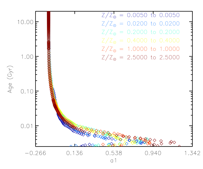
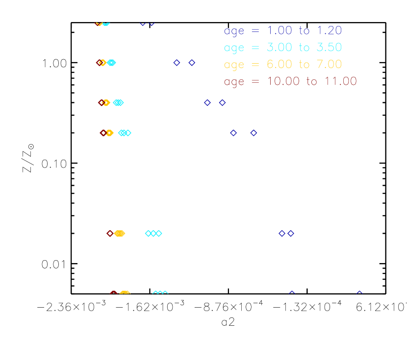
Figure 13: (Left) The dependence of stellar age on the first PCA  eigencoefficient of Region01, for different stellar metallicities. (Right) The dependence of stellar metallicity on the second PCA eigencoefficient, for different stellar ages, in the SDSS configuration. Although the relations are monotonic (except the smallest ages on the left), they are not straightly linear, which in turn explains the small correlation coefficient amplitude listed in Table 3. This result suggests that other (nonlinear) measures, rather than the Pearson correlation coefficient, may better describe the relation between the eigencoefficients and the physical parameters.

We then perform a PCA  on the cutouts from Region01  in the SDSS configuration and relate the eigencoefficients to stellar age and metallicity. The eigenspectra are shown in Appendix B. Focusing on the lowest orders of eigencoefficients, shown in Figure 13, the first eigencoefficient correlates well with the stellar age regardless of the stellar metallicity, and the second eigencoefficient with the stellar metallicity after the age is known. These results agree with those obtained from the parameter sensitivity analysis that are shown in the last few columns of Table 3. The determination of stellar age from the first eigencoefficient appears to work best for intermediate ages, which is not surprising considering the optical spectra of galaxies dominated by old ($>$ a few Gyr) stellar populations look alike, posing a well-known limitation on the determination of stellar age in galaxies from optical spectra. We also found a similar situation for galaxies dominated by very young populations ($<$ 10 Myr), where spectra of two different ages can show the same first-eigencoefficient amplitude. Interestingly, we have to know the stellar age before we can tell the stellar metallicity, in other words, they have to be determined simultaneously, which is a manifestation of the well-known ”age-metallicity degeneracy” problem (e.g., Faber, 1973; Mould, 1978; Schmidt et al., 1989) in galaxy parameter estimation. To conclude, we can use the regional eigencoefficients to determine the stellar age and metallicity in early-type galaxies which have solar abundance ratios, no dust, and a single-burst star formation history. It remains to be seen how the parameters which are relevant to late-type galaxies, such as the exponentially decreasing star formation rate and the dust extinction, depend on the eigencoefficients of a region.

5 Conclusions

We identify informative wavelength regions in a single-burst stellar populations model by using the CUR Matrix Decomposition  (Drineas et al., 2008; Mahoney & Drineas, 2009). The regions are objective. They are shown to be sensitive to stellar age and metallicity. The regions can be used to determine the stellar age and metallicity in early-type galaxies which have solar abundance ratios, no dust, and a single-burst star formation history. The region  identification method and the subspace analysis can be applied to any set of spectra of the user’s interest, so that we eliminate the need for a common, fixed resolution index system.

We plan to extend this analysis to late-type galaxies. The presence of emission lines pose special challenges to the region  identification on the whole spectra, namely, the continuum + absorption + emission spectra. This speculation is hinted by the fact that the continuum-included strong emission lines cannot be reconstructed with higher than $\approx{20}\%$ accuracy on average by using a handful of lower-order eigenspectra (Yip et al., 2004; Marchetti et al., 2012). We are investigating this question. A possible approach is that of Győry et al. (2011) who parameterized the continuum-subtracted emission-line EWs through a handful of eigenspectra. To this end, the SDSS galaxies will be a perfect dataset. Because of the many galaxy types, a large diversity in the emission lines and the associated gas kinematics can be studied. A set of regions, taken into account of both absorption and emission lines, will give a comprehensive parametrization to emission-line galaxy spectra. The progress on understanding galaxy parameters have already set benchmarks in the field (e.g., Kauffmann et al., 2003; Gallazzi et al., 2005; Wild et al., 2007; Chen et al., 2012). This work provides a factor of $\approx 100$ reduction over the original data. Such a data compression will be crucial if we want to estimate simultaneously a large number ($>10$) of galaxy parameters (Yip & Wyse, 2007; Yip, 2010) in the future, such as stellar age and metallicity, dust extinction, and high temporal resolution star formation history.

6 Acknowledgments

We thank Andrew Connolly, Haijun Tian, Miguel Angel Aragon Calvo, and Guangtun Zhu for useful comments and discussions. CWY thanks Scott Trager for discussions on galaxy spectra. We thank the referee for careful reading of the manuscript and useful suggestions.

This research is partly funded by the Gordon and Betty Moore Foundation through Grant GBMF#554.01 to the Johns Hopkins University. IC and LD acknowledge grant OTKA-103244. This research has made use of data obtained from or software provided by the US National Virtual Observatory, which is sponsored by the National Science Foundation.

Appendix A CUR Matrix Decomposition

The CUR Matrix Decomposition  (Drineas et al., 2008; Mahoney & Drineas, 2009) computes a low-rank approximation to an arbitrary matrix that marvels the optimal low-rank approximation provided by the truncated Singular Value Decomposition (SVD). The approximation, however, is expressed in terms of a small number of actual columns and/or rows of the input data matrix. That is, it captures the dominant modes of variation in a data matrix with a small number of actual (and thus potentially interpretable) columns and/or rows, rather than a small number of (in general non-interpretable) eigencolumns and eigenrows. The CUR Matrix Decomposition  has been used in Genetics to identify “PCA-correlated SNPs”, basically the most informative columns within DNA single-nucleotide polymorphism (SNP) matrices (Paschou et al., 2007); and it has been central to recent work in developing randomized algorithms for the low-rank approximation of very large matrices (Mahoney, 2011).

The main idea behind the CUR Matrix Decomposition is to decompose a given matrix $A$ into matrices $C$ and $R$ which consist of respectively a small number of actual columns and rows of $A$, and a low-dimensional encoding matrix $\mathbb{U}$, such that $A\approx C\mathbb{U}R$ as follows

$$\|A-C\mathbb{U}R\|_{F}\leq(1+\epsilon)\|A-A_{k}\|_{F},$$ (A1)

where $A_{k}$ is the best rank-$k$ approximation to $A$, as given by the truncated SVD. The fractional error of the decomposition is $\epsilon$. Subscript $F$ denotes the Frobenius norm of a matrix. We use only the column part of the decomposition in this paper. The choice of the columns is critical: to obtain low-rank approximation bounds of the form in Eqn. A1, one chooses columns randomly according to an importance sampling distribution that is proportional to the Leverage Scores (of $A$, relative to the best rank-$k$ approximation to $A$). These quantities, given in Eqn. 2, equal the diagonal elements of the projection matrix onto the span of the best rank-$k$ approximation to $A$. They have been used previously in regression diagnostics as a measure of the importance or influence a given data point has on the least-squares fit (Chatterjee & Hadi, 1986). When applied to low-rank matrix approximations, the Leverage Scores provide a measure of how informative is a given column to the best rank-$k$ approximation of the data matrix. In our case, a column is a wavelength in the model spectra.

Appendix B Regional Eigenspectra

The lowest orders of the eigenspectra encapsulate most of the sample variance in the full optical spectra of nearby galaxies (Yip et al., 2004), forming a subspace which lies in a higher-dimensional wavelength space. We examine here the first few orders of eigenspectra of Region01 in the SDSS configuration. Together with the mean spectrum of the model the eigenspectra are plotted in Figure 1. The third eigenspectrum shows an anti-correlation between the strengths of the Balmer and the Ca K & H absorptions. Wild et al. (2007) also found that the third mode modulates the Ca K & H strength, though the concerned model has an exponential star formation history with recent stellar bursts. We see from Figure 1 that the first and second eigenspectra modulate respectively the Balmer absorption and the 4000 Å break  strengths. On the other hand, we know from the parameter dependence in Figure 13 that first eigenspectrum of the single-burst stellar populations model tells primarily the stellar age. The second eigenspectrum is related to the age-metallicity degeneracy. We therefore conclude the following. The larger the first eigencoefficient of a galaxy spectrum, the stronger the Balmer absorptions, indicating the stellar populations are younger. The larger the second eigencoefficient, the stronger the 4000 Å break, indicating the stellar populations are either older and less metal rich, or younger and more metal rich.

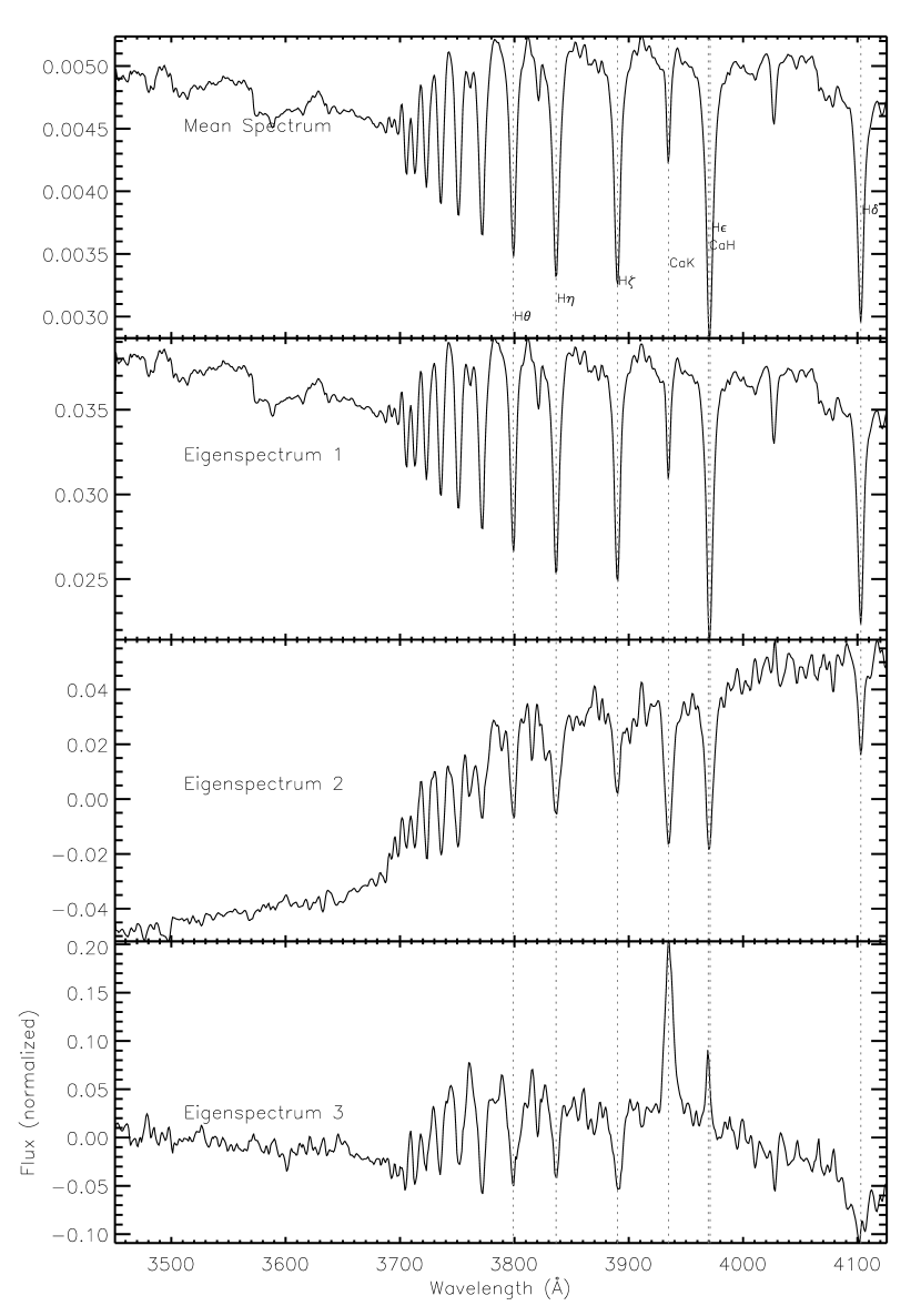
Figure 1: The mean spectrum (top) and first three eigenspectra of Region01 in the SDSS configuration. The first eigenspectrum modulates the Balmer absorption  strength (i.e., the stellar age). The second eigenspectrum modulates the 4000 Å break  strength (i.e., the age-metallicity degeneracy). The third eigenspectrum shows an anti-correlation between the strengths of the Balmer and the Ca K & H absorptions.

Table 1: LeverageScoreSum of Extended Lick/IDS indices, for wavelength range 3800–6400 Å at 9 Å spectral resolution.

Region	Reference	Unit	$\lambda_{S}$	$\lambda_{E}$	$\lambda_{E}-\lambda_{S}$	$\sum p_{\lambda}$
Dn(4000)	Balogh99	N/A	[3851.1, 4001.1]	[3951.1, 4101.2]	[100.0, 100.0]	0.199
H$\beta$	Trager98	Å	4849.2	4878.0	28.8	0.050
H$\delta_{A}$	WortheyOttaviani97	Å	4084.7	4123.4	38.8	0.040
G4300	Trager98	Å	4282.6	4362.6	80.0	0.039
C24668	Trager98	Å	4635.3	4721.6	86.3	0.027
H$\delta_{F}$	WortheyOttaviani97	Å	4092.2	4113.4	21.3	0.027
H$\gamma_{A}$	WortheyOttaviani97	Å	4321.0	4364.7	43.8	0.026
TiO2	Trager98	mag	6191.3	6273.9	82.5	0.021
Fe4531	Trager98	Å	4515.5	4560.5	45.0	0.021
Fe4383	Trager98	Å	4370.4	4421.6	51.3	0.019
H$\gamma_{F}$	WortheyOttaviani97	Å	4332.5	4353.5	21.0	0.018
Mg2	Trager98	mag	5155.6	5198.1	42.5	0.018
CN2	Trager98	mag	4143.3	4178.3	35.0	0.018
CN1	Trager98	mag	4143.3	4178.3	35.0	0.018
Ca4455	Trager98	Å	4453.4	4475.9	22.5	0.018
Fe5015	Trager98	Å	4979.1	5055.4	76.3	0.016
Mgb	Trager98	Å	5161.6	5194.1	32.5	0.016
NaD	Trager98	Å	5878.5	5911.0	32.5	0.012
Mg1	Trager98	mag	5070.5	5135.6	65.0	0.011
TiO1	Trager98	mag	5938.3	5995.8	57.5	0.009
Fe5270	Trager98	Å	5247.1	5287.1	40.0	0.008
Fe5406	Trager98	Å	5389.0	5416.5	27.5	0.007
Fe5335	Trager98	Å	5313.6	5353.6	40.0	0.005
Ca4227	Trager98	Å	4223.4	4235.9	12.5	0.004
Fe5709	Trager98	Å	5698.2	5722.0	23.8	0.004
Fe5782	Trager98	Å	5778.2	5798.2	20.0	0.003

Table 2: Informative wavelength regions, for wavelength range 3800–6400 Å at 9 Å spectral resolution.

Region	$\lambda_{S}$	$\lambda_{I}$	$\lambda_{E}$	$\lambda_{E}-\lambda_{S}$	$\lambda_{I}-\lambda_{S}$	Symmetric?	$\sum p_{\lambda}$	Lick/IDS Overlaps	1st mode	$u^{1}\cdot$ $p$	2nd mode	$u^{2}\cdot$ $p$
Region01	3801.2	3932.5	4053.8	252.5	131.2	no	0.312	Dn(4000)L;Dn(4000)R;	AGE	-0.395	METAL	-0.135
Region02	4761.2	4856.2	4908.8	147.5	95.0	no	0.104	H$\beta$;	AGE	-0.393	METAL	-0.163
Region03	4080.0	4101.2	4183.8	103.8	21.2	no	0.075	CN1;CN2;H$\delta_{A}$;H$\delta_{F}$;Dn(4000)R;	AGE	-0.396	AGE	0.208
Region12	4497.5	4505.0	4548.8	51.2	7.5	no	0.028	Fe4531;	AGE	-0.397	AGE	0.054
Region05	4321.2	4340.0	4351.2	30.0	18.8	no	0.022	G4300;H$\gamma_{A}$;H$\gamma_{F}$;	AGE	-0.392	AGE	0.120
Region04	4461.2	4470.0	4486.2	25.0	8.8	no	0.020	Ca4455;	AGE	-0.398	METAL	-0.277
Region06	5162.5	5167.5	5188.8	26.2	5.0	no	0.015	Mg2;Mgb;	AGE	-0.388	METAL	0.166
Region08	4636.2	4648.8	4652.5	16.2	12.5	no	0.010	C24668;	AGE	-0.394	METAL	-0.274
Region11	5885.0	5891.2	5901.2	16.2	6.2	no	0.008	NaD;	AGE	-0.374	AGE	0.073
Region13	4061.2	4071.2	4078.8	17.5	10.0	no	0.008	Dn(4000)R;	AGE	-0.398	METAL	-0.333
Region10	4191.2	4198.8	4202.5	11.2	7.5	no	0.007	$\cdots$	AGE	-0.397	METAL	0.263
Region15	4292.5	4300.0	4308.8	16.2	7.5	no	0.007	G4300;	AGE	-0.398	METAL	0.155
Region16	4257.5	4266.2	4273.8	16.2	8.8	no	0.007	$\cdots$	AGE	-0.397	METAL	-0.140
Region09	4381.2	4387.5	4391.2	10.0	6.2	no	0.007	Fe4383;	AGE	-0.398	METAL	-0.174
Region07	4913.8	4921.2	4923.8	10.0	7.5	no	0.006	$\cdots$	AGE	-0.393	METAL	-0.349
Region17	5262.5	5265.0	5272.5	10.0	2.5	no	0.005	Fe5270;	AGE	-0.388	METAL	-0.043
Region20	5872.5	5876.2	5883.8	11.2	3.8	no	0.004	NaD;	AGE	-0.375	METAL	0.244
Region14	4411.2	4415.0	4420.0	8.8	3.8	no	0.004	Fe4383;	AGE	-0.399	AGE	-0.097
Region18	4311.2	4315.0	4317.5	6.2	3.8	no	0.003	G4300;	AGE	-0.398	METAL	-0.154
Region19	4393.8	4395.0	4398.8	5.0	1.2	no	0.002	Fe4383;	AGE	-0.399	METAL	-0.139

The regions are sorted by the LeverageScoreSum amplitude. If $\lambda_{I}-\lambda_{S}=\lambda_{E}-\lambda_{I}$, the region is called symmetric. AGE stands for stellar age, METAL for stellar metallicity. The vector $p$ is either the AGE or METAL in the object space, as that indicated in the columns “1st mode” and “2nd mode”. The vector $u$ is the left singular vector of that region. The dot product between them, performed in the object space, tells how correlated the singular vector is to the corresponding parameter. In both the “1st mode” and “2nd mode” columns, only the parameter which is most correlated with the singular vector is shown. The extra horizontal line divides the regions with LeverageScoreSum less than and larger than 0.03.

Table 3: Informative wavelength regions, for wavelength range 3450–8350 Å at 3 Å spectral resolution.

Region	$\lambda_{S}$	$\lambda_{I}$	$\lambda_{E}$	$\lambda_{E}-\lambda_{S}$	$\lambda_{I}-\lambda_{S}$	Symmetric?	$\sum p_{\lambda}$	Lick/IDS Overlaps	1st mode	$u^{1}\cdot$ $p$	2nd mode	$u^{2}\cdot$ $p$
Region01	3450.8	3934.5	4125.6	674.8	483.8	no	0.403	H$\delta_{A}$;H$\delta_{F}$;Dn(4000)L;Dn(4000)R;	AGE	-0.390	METAL	-0.079
Region08	4378.0	4472.7	4574.7	196.8	94.7	no	0.063	Fe4383;Ca4455;Fe4531;	AGE	-0.397	METAL	-0.137
Region03	4773.7	4861.3	4899.5	125.8	87.6	no	0.056	H$\beta$;	AGE	-0.393	METAL	-0.171
Region04	4238.2	4340.9	4377.0	138.8	102.7	no	0.049	G4300;Fe4383;H$\gamma_{A}$;H$\gamma_{F}$;	AGE	-0.396	METAL	-0.177
Region14	4135.1	4144.6	4237.2	102.1	9.5	no	0.028	CN1;CN2;Ca4227;	AGE	-0.398	METAL	-0.220
Region12	4594.8	4651.2	4656.5	61.7	56.4	no	0.015	C24668;	AGE	-0.395	METAL	-0.255
Region02	6549.4	6564.5	6576.6	27.2	15.1	no	0.012	$\cdots$	AGE	-0.371	METAL	0.253
Region09	8219.7	8229.2	8259.5	39.8	9.5	no	0.009	$\cdots$	AGE	-0.370	METAL	0.290
Region10	7166.1	7187.6	7197.5	31.4	21.5	no	0.008	$\cdots$	AGE	-0.375	METAL	0.305
Region06	5165.9	5168.2	5179.0	13.1	2.4	no	0.006	Mg2;Mgb;	AGE	-0.388	METAL	0.157
Region11	5887.3	5892.8	5902.3	14.9	5.4	no	0.006	NaD;	AGE	-0.374	METAL	0.093
Region19	4914.2	4924.4	4936.9	22.7	10.2	no	0.006	$\cdots$	AGE	-0.393	METAL	-0.388
Region18	8159.4	8178.2	8182.0	22.6	18.8	no	0.005	$\cdots$	AGE	-0.373	METAL	0.301
Region17	4681.3	4686.6	4694.2	12.9	5.4	no	0.004	C24668;	AGE	-0.393	AGE	0.035
Region07	4712.6	4714.8	4720.2	7.6	2.2	no	0.003	C24668;	AGE	-0.393	METAL	0.428
Region20	5180.2	5183.7	5189.7	9.5	3.6	no	0.003	Mg2;Mgb;	AGE	-0.387	METAL	0.164
Region13	5224.5	5226.9	5231.7	7.2	2.4	no	0.003	$\cdots$	AGE	-0.387	METAL	0.121
Region05	8090.2	8092.1	8097.7	7.5	1.9	no	0.003	$\cdots$	AGE	-0.364	METAL	-0.121
Region16	7274.1	7277.4	7279.1	5.0	3.3	no	0.002	$\cdots$	AGE	-0.375	METAL	0.335
Region15	5053.0	5054.1	5056.5	3.5	1.2	no	0.002	Fe5015;	AGE	-0.391	METAL	-0.143

See footnote in Table 2.

Table 4: Informative wavelength regions, for wavelength range 3450–8350 Å at 3 Å spectral resolution, continued.

Region	$\sum p_{\lambda}$	Lick/IDS Overlaps	Optical Line Overlaps
Region01	0.403	H$\delta_{A}$;H$\delta_{F}$;Dn(4000)L;Dn(4000)R;	H$\theta$$\lambda$3799;H$\eta$$\lambda$3836;H$\zeta$$\lambda$3890;CaK$\lambda$3935;CaH$\lambda$3970;H$\epsilon$$\lambda$3971;H$\delta$$\lambda$4103;
Region08	0.063	Fe4383;Ca4455;Fe4531;	$\cdots$
Region03	0.056	H$\beta$;	H$\beta$$\lambda$4863;
Region04	0.049	G4300;Fe4383;H$\gamma_{A}$;H$\gamma_{F}$;	H$\gamma$$\lambda$4342;
Region14	0.028	CN1;CN2;Ca4227;	$\cdots$
Region12	0.015	C24668;	$\cdots$
Region02	0.012	$\cdots$	H$\alpha$$\lambda$6565;
Region09	0.009	$\cdots$	$\cdots$
Region10	0.008	$\cdots$	$\cdots$
Region06	0.006	Mg2;Mgb;	MgI$\lambda$5169;MgI$\lambda$5174;
Region11	0.006	NaD;	NaI$\lambda$5892;NaI$\lambda$5898;
Region19	0.006	$\cdots$	$\cdots$
Region18	0.005	$\cdots$	$\cdots$
Region17	0.004	C24668;	$\cdots$
Region07	0.003	C24668;	$\cdots$
Region20	0.003	Mg2;Mgb;	$\cdots$
Region13	0.003	$\cdots$	$\cdots$
Region05	0.003	$\cdots$	$\cdots$
Region16	0.002	$\cdots$	$\cdots$
Region15	0.002	Fe5015;	$\cdots$

This table lists the Lick/IDS indices, and the prominent optical absorption lines, which overlap with the identified regions.

Figure 3: The width of the Na D-region as a function of $k$, for $T$= 0.7  in the Lick/IDS configuration. The width converges.

Figure 6: The width of the Na D-region as a function of $k$, for $T$= 0.7  in the SDSS configuration. The width converges.

References

- Balogh et al. (1999) Balogh, M. L., Morris, S. L., Yee, H. K. C., Carlberg, R. G., & Ellingson, E. 1999, ApJ, 527, 54
- Bruzual A. (1983) Bruzual A., G. 1983, ApJ, 273, 105
- Bruzual & Charlot (2003) Bruzual, G., & Charlot, S. 2003, MNRAS, 344, 1000
- Budavári et al. (2009) Budavári, T., Wild, V., Szalay, A. S., Dobos, L., & Yip, C.-W. 2009, MNRAS, 394, 1496
- Burstein et al. (1984) Burstein, D., Faber, S. M., Gaskell, C. M., & Krumm, N. 1984, ApJ, 287, 586
- Chabrier (2003) Chabrier, G. 2003, PASP, 115, 763
- Chatterjee & Hadi (1986) Chatterjee S. & Hadi A. S. 1986, Statistical Science, 1, 379-393
- Chen et al. (2012) Chen, Y.-M., Kauffmann, G., Tremonti, C. A., et al. 2012, MNRAS, 421, 314
- Connolly et al. (1995) Connolly, A. J., Szalay, A. S., Bershady, M. A., Kinney, A. L., & Calzetti, D. 1995, AJ, 110, 1071
- Dobos et al. (2012) Dobos, L., Csabai, I., Yip, C.-W., et al. 2012, MNRAS, 420, 1217
- Drineas et al. (2008) Drineas P., Mahoney M. W., & Muthukrishnan S. 2008, SIAM. J. Matrix Anal. & Appl., 30, 844
- Faber (1973) Faber, S. M. 1973, ApJ, 179, 731
- Faber et al. (1985) Faber, S. M., Friel, E. D., Burstein, D., & Gaskell, C. M. 1985, ApJS, 57, 711
- Francis et al. (1992) Francis, P. J., Hewett, P. C., Foltz, C. B., & Chaffee, F. H. 1992, ApJ, 398, 476
- Gallazzi et al. (2005) Gallazzi, A., Charlot, S., Brinchmann, J., White, S. D. M., & Tremonti, C. A. 2005, MNRAS, 362, 41
- Girardi et al. (1996) Girardi, L., Bressan, A., Chiosi, C., Bertelli, G., & Nasi, E. 1996, A&AS, 117, 113
- Gorgas et al. (1993) Gorgas, J., Faber, S. M., Burstein, D., Gonzalez, J. J., Courteau, S., & Prosser, C. 1993, ApJS, 86, 153
- Gunawan, Neswan, & Setya-Budhi (2005) Gunawan, H., Newwan, O., & Setya-Budhi, W. 2005, Contributions to Algebra and Geometry, 46, 331
- Győry et al. (2011) Győry, Z., Szalay, A. S., Budavári, T., Csabai, I., & Charlot, S. 2011, AJ, 141, 133
- Jones & Worthey (1995) Jones, L. A., & Worthey, G. 1995, ApJ, 446, L31
- Kauffmann et al. (2003) Kauffmann, G., et al. 2003, MNRAS, 341, 33
- Krughoff et al. (2011) Krughoff, K. S., Connolly, A. J., Frieman, J., SubbaRao, M., Kilper, G., & Schneider, D. P. 2011, ApJ, 731, 42
- Marchetti et al. (2012) Marchetti, A., Granett, B. R., Guzzo, L., et al. 2012, arXiv:1207.4374
- Madgwick et al. (2003) Madgwick, D. S., Hewett, P. C., Mortlock, D. J., & Wang, L. 2003, ApJ, 599, L33
- Mahoney & Drineas (2009) Mahoney M. W. & Drineas P. 2009, Proc. Natl. Acad. Sci. USA, 106, 697-702
- Mahoney (2011) Mahoney, M. W. 2011, arXiv:1104.5557
- Mould (1978) Mould, J. R. 1978, ApJ, 220, 434
- Paschou et al. (2007) Paschou P., Ziv E., Burchard E. G., Choudhry S., Rodriguez-Cintron W., Mahoney M. W. & Drineas P. 2007, PLoS Genetics, 3, 1672-1686
- Sánchez Almeida et al. (2012) Sánchez Almeida, J., Terlevich, R., Terlevich, E., Cid Fernandes, R., & Morales-Luis, A. B. 2012, ApJ, 756, 163
- Schiavon (2007) Schiavon, R. P. 2007, ApJS, 171, 146
- Schmidt et al. (1989) Schmidt, A. A., Bica, E., & Dottori, H. A. 1989, MNRAS, 238, 925
- Shang et al. (2003) Shang, Z., Wills, B. J., Robinson, E. L., et al. 2003, ApJ, 586, 52
- Strang (1988) Strang, G. 1988, Linear Algebra and Its Application, 3rd edition, Harcourt Brace Jovanovich, Publishers
- Thomas et al. (2004) Thomas, D., Maraston, C., & Korn, A. 2004, MNRAS, 351, L19
- Trager et al. (1998) Trager, S. C., Worthey, G., Faber, S. M., Burstein, D., & Gonzalez, J. J. 1998, ApJS, 116, 1
- Vanden Berk et al. (2006) Vanden Berk, D. E., et al. 2006, AJ, 131, 84
- Wild & Hewett (2005) Wild, V., & Hewett, P. C. 2005, MNRAS, 358, 1083
- Wild et al. (2007) Wild, V., Kauffmann, G., Heckman, T., et al. 2007, MNRAS, 381, 543
- Worthey et al. (1992) Worthey, G., Faber, S. M., & Gonzalez, J. J. 1992, ApJ, 398, 69
- Worthey et al. (1994) Worthey, G., Faber, S. M., Gonzalez, J. J., & Burstein, D. 1994, ApJS, 94, 687
- Worthey & Ottaviani (1997) Worthey, G., & Ottaviani, D. L. 1997, ApJS, 111, 377
- Yip et al. (2004) Yip, C. W., et al. 2004, AJ, 128, 585
- Yip et al. (2004) Yip, C. W., et al. 2004, AJ, 128, 2603
- Yip & Wyse (2007) Yip, C.-W., & Wyse, R. F. G. 2007, IAU Symposium, 241, 533
- Yip (2010) Yip, C.-W. 2010, AJ, 139, 342
- York et al. (2000) York, D. G., Adelman, J., Anderson, J. E., Jr., et al. 2000, AJ, 120, 1579