Coleman-de Luccia instanton in dRGT massive gravity

Abstract

We study the Coleman-de Luccia (CDL) instanton characterizing the tunneling from a false vacuum to the true vacuum in a semi-classical way in dRGT (deRham-Gabadadze-Tolley) massive gravity theory, and evaluate the dependence of the tunneling rate on the model parameters. It is found that provided with the same physical Hubble parameters for the true vacuum $H_{\rm T}$ and the false vacuum $H_{\rm F}$ as in General Relativity (GR), the thin-wall approximation method implies the same tunneling rate as GR. However, deviations of tunneling rate from GR arise when one goes beyond the thin-wall approximation and they change monotonically until the Hawking-Moss (HM) case. Moreover, under the thin-wall approximation, the HM process may dominate over the CDL one if the value for the graviton mass is larger than the inverse of the radius of the bubble.

I Introduction

The notion of gravitational theory with a massive graviton is nothing new. A massive gravity theory was firstly proposed by Fierz and Pauli (FP) in 1939 where the theory of General Relativity (GR) was extended by a linear mass term Fierz:1939 . However, lack of Hamiltonian and momentum constraints leads to 6 degrees of freedom in this theory, with 5 of which corresponding to those of a massive spin-2 graviton and the rest one a Boulware-Deser (BD) ghost mode Boulware:1972 ; Creminelli:2005qk ; Rubakov:2008 ; Hinterbichler:2012 . A breakthrough was achieved by recent development of de Rham-Gabadadze-Tolley (dRGT) nonlinear massive gravity theory Rham:2010 ; Rham:2011PRL ; Hassan:2011vm , where a special form of potential was introduced to recover the Hamiltonian constraint so that the sixth BD ghost mode is eliminated Hassan:2012 ; Hassan:2011tf . One of the most remarkable consequences in this theory is that it allows self-accelerating solutions D'Amico:2011jj ; Gumrukcuoglu:2011open ; Kobayashi:2012 ; Gratia:2012 , where the universe takes the de Sitter form even without a bare cosmological constant, and its Hubble scale is of the order of the graviton mass.

However, application of the self-accelerating solution to explain the current accelerated expansion of universe does not solve the “Cosmological Constant Problem” (CCP) Weinberg:1988cp ; Nobbenhuis:2004wn , which implies a serious contradiction between smallness of the cosmological constant and expected large quantum corrections. Motivated by the proposal that CCP may hopefully be solved by the anthropic selection of the cosmological constant in the landscape of vacua Weinberg:1988cp ; Susskind:2003kw ; Nobbenhuis:2004wn , the Hawking-Moss (HM) solution Hawking:1981fz in dRGT massive gravity was studied in ZSS:2013 . It was found that depending on the choice of parameters in dRGT massive gravity theory, the non-vanishing mass of a graviton will influence the tunneling rate of HM instanton, hence affects the stability of a vacuum in this theory.

On the other hand, it was known that in GR, traditionally, the Hartle-Hawking (HH) no-boundary wavefunction Hartle:1983 exponentially prefers small number of $e$-foldings near the minimum of the inflaton potential, hence it does not seem to predict the universe we observe today. Such situation may be drastically changed by application of the correction term in the Euclidean HM action to HH no-boundary proposal. It was found that for a wide range choice of the parameters in dRGT massive gravity theory, the no-boundary wavefunction can peak at a sufficiently large value of the Hubble parameter, hence one may obtain a sufficient number of $e$-folds of inflation SYZ:2013 .

Inspired by these interesting achievements, as a necessary step towards understanding of tunneling process in dRGT massive gravity theory, it is necessary to explore another kind of phase transition in theories of scalar fields coupled to gravity: Coleman-de Luccia (CDL) instanton that exists for a special form of potentials such that the curvature scale of the barrier is large compared to the potential energy (in Planck units) Coleman:1980 ; BK:2006 , and gradually approaches to the HM instanton as the curvature scale shrinks. In this paper, we consider the CDL solution for a scalar field with minimal coupling to gravity in dRGT massive gravity theory. We set up the model and found the bounce solutions corresponding to the CDL instantons. Based on these solutions, we evaluate the CDL action in two approaches: “thin-wall” approximation and perturbations around HM solution, and find monotonic contributions from the graviton mass terms until the “thick-wall” limit: the HM case. Moreover, in the “thin-wall” limit, comparison of the tunneling rates for the HM and CDL solutions with the same potential shows that, even when the CDL process dominates over the HM one in the case of GR, it may behave inversely in the context of dRGT massive gravity, i.e. depending on the values of parameters in this model, the HM process may dominate over the CDL one.

This paper is organized as follows. In Sec. II, we setup the Lagrangian for our model. In Sec. III, we formulate the equations of motion (EOM) and solve the constraint equation. In Sec. IV, the CDL solution is studied by using “thin-wall” approximation. In Sec. V, we study the CDL solution as perturbations around the Hawking-Moss (HM) solution obtained in Ref. ZSS:2013 and clarify its relationship with the one obtained by “thin-wall” approximation. In Sec. VI, we compare the tunneling rates for the CDL and HM instantons for the same potential which satisfies the condition for “thin-wall” approximation. In Sec. VII, we draw the conclusions. In Appendix. A, we present the detailed calculations of the CDL process as perturbations around HM one. Appendix. B is devoted to the deduction of comparison of the CDL to HM probabilities.

Throughout the paper, the Lorentzian metric signature is set to be $(-,+,+,+)$, while the Euclidean metric signature $(+,+,+,+)$. Meanwhile, we use the conventional notations where indices with Greek letters $\mu,\nu,...$ for the spacetime indices, the Latin letters $i,j,...$ for the space indices, while the Latin indices $a,b,...$ for the internal space (Lorentz frame) indices. Also repeated indices imply the summation unless otherwise stated.

II Setup of model

We study the tunneling process of a minimally coupled scalar field $\sigma$ which tunnels from one vacua $\sigma_{\rm F}$ to another one $\sigma_{\rm T}$ in the context of dRGT massive gravity, as illustrated in Fig. 1. The dRGT massive gravity is composed of two metrics, namely a physical metric $g_{\mu\nu}$ and a fiducial metric $G_{ab}$, with the Stückelberg fields $\phi^{a}$ Rham:2010 ; Rham:2011PRL . As usual, the whole action can be divided into two parts: the nonlinear massive gravity part $I_{g}$ and the minimally coupled scalar field part $I_{m}$ as follows:

$$S =I_{g}+I_{m},$$ (1)

$$I_{g} \equiv\int\mathrm{d}^{4}x~{}\sqrt{-g}\left[\frac{R}{2}+m_{g}^{2}(\mathcal{L}_{2}+\alpha_{3}\mathcal{L}_{3}+\alpha_{4}\mathcal{L}_{4})\right],$$ (2)

$$I_{m} \equiv-\int\mathrm{d}^{4}x~{}\sqrt{-g}\left[\frac{1}{2}(\partial\sigma)^{2}+V(\sigma)\right],$$ (3)

where $m_{g}$, $\alpha_{3}$ and $\alpha_{4}$ are three free parameters in this model, and

$${\cal L}_{2} =\frac{1}{2}\left(\left[{\cal K}\right]^{2}-\left[{\cal K}^{2}\right]\right)\,,$$

$${\cal L}_{3} =\frac{1}{6}\left(\left[{\cal K}\right]^{3}-3\left[{\cal K}\right]\left[{\cal K}^{2}\right]+2\left[{\cal K}^{3}\right]\right),$$

$${\cal L}_{4} =\frac{1}{24}\left(\left[{\cal K}\right]^{4}-6\left[{\cal K}\right]^{2}\left[{\cal K}^{2}\right]+3\left[{\cal K}^{2}\right]^{2}+8\left[{\cal K}\right]\left[{\cal K}^{3}\right]-6\left[{\cal K}^{4}\right]\right),$$ (4)

with

$${\cal K}^{\mu}_{\nu}\equiv\delta^{\mu}_{\nu}-\sqrt{g^{\mu\sigma}G_{ab}(\phi)\partial_{\nu}\phi^{a}\partial_{\sigma}\phi^{b}}.$$ (5)

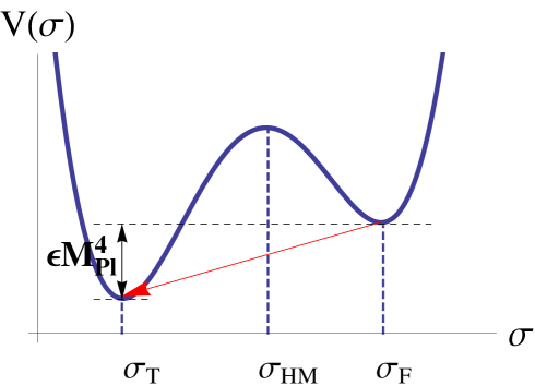
Figure 1: Illustration of the potential $V(\sigma)$ with two local minima $\sigma_{\rm F}$ and $\sigma_{\rm T}$, which correspond to the false and true vacuum respectively, while $\sigma_{\rm HM}$ labels its local maximum value. In the thin-wall approximation, the difference of the potential values at these two local minima is very small, i.e. $V(\sigma_{\rm F})-V(\sigma_{\rm T})=\epsilon\ll 1$.

In order to investigate tunneling process, the potential $V(\sigma)$ is assumed to have two local minima $\sigma_{\rm F}$ and $\sigma_{\rm T}$ which correspond to the false and true vacuum, respectively, with a local maximum between them, $\sigma=\sigma_{\rm HM}$, as illustrated in Fig. 1.

The Euclidean action of (1) is obtained by Wick rotation $x^{0}\to ix_{\rm E}^{0}$ and correspondingly $S_{\rm E}=iS$. In the semiclassical limit, the tunneling rate per unit time per unit volume can be expressed in terms of the Euclidean action as follows:

$$P\equiv\Gamma/V=Ae^{-B}\,;\quad B=S_{\rm E}[{g}_{\mu\nu,{\rm B}},{\phi}_{\rm B}]-S_{\rm E}[{g}_{\mu\nu,{\rm F}},{\phi}_{\rm F}]\,,$$ (6)

where $\{{g}_{\mu\nu,{\rm B}},{\phi}_{\rm B}\}$ is the bounce solution, which is a solution of the Euclidean equations of motion with appropriate boundary conditions, and $\{{g}_{\mu\nu,{\rm F}},{\phi}_{\rm F}\}$ is the solution of false vacuum Coleman:1980 . Conventionally, the bounce solution $\{{g}_{\mu\nu,{\rm B}},{\phi}_{\rm B}\}$ is explored under the assumption of $O(4)$-symmetry, since an $O(4)$-symmetric solution gives the lowest action for a wide class of scalar-field theories, hence gives the least value of action which dominates the tunneling process Coleman:1977th ; Lee:2008 ; Lee:2009 ; Lee:2011 ; Lee:2013 . The same assumption is also reasonable in the presence of gravity Coleman:1980 , therefore, the physical metric can be assumed to take the following form,

$$g_{\mu\nu}\mathrm{d}x^{\mu}\mathrm{d}x^{\nu}=N(\xi)^{2}\mathrm{d}\xi^{2}+a(\xi)^{2}\Omega_{ij}\mathrm{d}x^{i}\mathrm{d}x^{j},$$ (7)

where $\Omega_{ij}\mathrm{d}x^{i}\mathrm{d}x^{j}$ is the metric on a three-sphere with $K>0$,

$$\Omega_{ij} \equiv\delta_{ij}+\frac{K\delta_{il}\delta_{jm}x^{l}x^{m}}{1-K\delta_{lm}x^{l}x^{m}}\,.$$ (8)

In the context of dRGT massive gravity, the fiducial metric $G_{ab}$ is assumed to be non-dynamical Hassan:2011zd ; Volkov:2011an ; Comelli:2011zm . In order to guarantee the $O(4)$-symmetry, we assume that it is given by the de Sitter metric Langlois:2012hk with a constant Hubble parameter $F$ ZSS:2013 :

$$G_{ab}(\phi)\mathrm{d}\phi^{a}\mathrm{d}\phi^{b} \equiv-(\mathrm{d}\phi^{0})^{2}+b(\phi^{0})^{2}\Omega_{ij}\mathrm{d}\phi^{i}\mathrm{d}\phi^{j},$$ (9)

where

$$\left\{\begin{aligned} b(\phi^{0})&\equiv F^{-1}\sqrt{K}\cosh(F\phi^{0})\,,\\ \phi^{0}&=f(\xi)\,,\quad\phi^{i}=x^{i}\,.\end{aligned}\right.$$ (10)

It should be noted that here we stick to the Lorentzian signature for the fiducial metric since it is non-dynamical in dRGT massive gravity theory. Nevertheless, thanks to the assumption of the de Sitter fiducial metric, we may adopt the $O(4)$-ansatz.

III Euclidean equations of motion

In this section, we present the Euclidean equations of motion. More detailed deductions can be found in ZSS:2013 .

Inserting the $O(4)$-ansatz (7) and (10) into (5), one obtains the Euclidean version of the action (11)

$$S_{\rm E} =I_{g{\rm E}}+I_{m{\rm E}},$$ (11)

where the gravity action is reduced to

$$I_{g{\rm E}}=\int\mathrm{d}^{4}x_{E}~{}\sqrt{\Omega}\left[-3KNa-\frac{3\dot{a}^{2}a}{N}-m_{g}^{2}\left(\mathcal{L}_{2E}+\alpha_{3}\mathcal{L}_{3E}+\alpha_{4}\mathcal{L}_{4E}\right)\right],$$ (12)

with

$$\mathcal{L}_{2E} =3a(a-b)\left(2Na-\sqrt{-\dot{f}^{2}}a-Nb\right),$$ (13a)

$$\mathcal{L}_{3E} =(a-b)^{2}\left(4Na-3\sqrt{-\dot{f}^{2}}a-Nb\right),$$ (13b)

$$\mathcal{L}_{4E} =(a-b)^{3}\left(N-\sqrt{-\dot{f}^{2}}\right),$$ (13c)

and a dot means a derivative with respect to the radial coordinate, $\dot{~{}}\equiv\mathrm{d}/\mathrm{d}\xi$. Meanwhile, the action for the tunneling field is reduced to

$$I_{mE}=\int\mathrm{d}^{4}x~{}a^{3}\sqrt{\Omega}\left[\frac{1}{2N}\dot{\sigma}^{2}+NV(\sigma)\right].$$ (14)

Variation of the action (12) with respect to the Stückelberg field $\phi^{0}=f$ gives the following constraint equation:

$$(i\dot{a}+Nb_{,f})\left[\left(3-\frac{2b}{a}\right)+\alpha_{3}\left(1-\frac{b}{a}\right)\left(3-\frac{b}{a}\right)+\alpha_{4}\left(1-\frac{b}{a}\right)^{2}\right]=0\,,$$ (15)

where $b_{,f}\equiv{\rm d}b/{\rm d}f=\sqrt{K}\sinh(Ff)$. Correspondingly, we obtain two branches:

$${\rm Branch~{}I}~{}\qquad\qquad Nb_{,f}=-i\dot{a}\,,$$ (16)

$${\rm Branch~{}II}~{}\qquad\left(3-\frac{2b}{a}\right)+\alpha_{3}\left(1-\frac{b}{a}\right)\left(3-\frac{b}{a}\right)+\alpha_{4}\left(1-\frac{b}{a}\right)^{2}=0\,.$$ (17)

In Branch I, it is known that there exists a tension between the Vainstein mechanism and the Higuchi bound Rham:2012p . This situation is not improved even in the extended massive gravity theories or bigravity theory. Hence, in the following, we mainly concentrate on analysis of Branch II. The solution to Eq. (17) is given by

$$b=X_{\pm}a\,,\qquad X_{\pm}\equiv\frac{1+2\,\alpha_{3}+\alpha_{4}\pm\sqrt{1+\alpha_{3}+\alpha_{3}^{2}-\alpha_{4}}}{\alpha_{3}+\alpha_{4}}\,,$$ (18)

where it should be noted that we require $X_{\pm}>0$ for our interest. Hereafter, for definiteness, the choice of $X_{+}$ is called Branch II₊ while $X_{-}$ is called Branch II_-. On the other hand, variations of the action (11) with respect to lapse function $N$ and $\sigma$ give the “Friedman equation” and field equation respectively:

$$\frac{3}{a^{2}}\left(a^{\prime 2}-K\right)=\frac{\sigma^{\prime 2}}{2}-V(\sigma)-\Lambda_{\pm}\,,$$ (19)

$$\sigma^{\prime\prime}+3\mathcal{H}\sigma^{\prime}-V_{,\sigma}(\sigma)=0\,,$$ (20)

where we have introduced the proper radial coordinate $\tau\equiv\int N{\rm d}\xi$ and a prime means derivative with respect to the proper time: $~{}^{\prime}\equiv{\rm d}/{\rm d}\tau$, $\mathcal{H}\equiv a^{\prime}/a$, while

$$\Lambda_{\pm} \equiv-m_{g}^{2}\left(1-X_{\pm}\right)\left[3\left(2-X_{\pm}\right)+\alpha_{3}\left(1-X_{\pm}\right)\left(4-X_{\pm}\right)+\alpha_{4}\left(1-X_{\pm}\right)^{2}\right]$$

$$=-\frac{m_{g}^{2}}{\left(\alpha_{3}+\alpha_{4}\right)^{2}}\left[\left(1+\alpha_{3}\right)\left(2+\alpha_{3}+2\,\alpha_{3}^{2}-3\,\alpha_{4}\right)\pm 2\,\left(1+\alpha_{3}+\alpha_{3}^{2}-\alpha_{4}\right)^{3/2}\right]\,.$$ (21)

As explained in the previous section, the tunneling rate (6) is given by the Euclidean action evaluated for a solution of Eqs. (19) and (20). In the following, we construct the CDL solution and then evaluate the action for it.

IV Coleman-DeLuccia solution from thin-wall approximation

IV.1 Expression for Euclidean action

In order to evaluate the CDL solution by using thin-wall approximation, one should firstly solve the Euclidean Friedmann equation (19) at the locally minimal point $\sigma_{\rm{T}}$ and the globally minimal point $\sigma_{\rm{F}}$ separately:

$$\frac{3}{a^{2}}\left(a^{\prime 2}-K\right)=\left\{\begin{aligned} &-V(\sigma_{\rm T})-\Lambda_{\pm}\equiv-\Lambda_{\pm,\rm{T}}\,,\qquad\tau<\tau_{0}\\ \\ &-V(\sigma_{\rm F})-\Lambda_{\pm}\equiv-\Lambda_{\pm,\rm{F}}\,,\qquad\tau>\tau_{0}\end{aligned}\right.$$ (22)

where $\tau_{0}$ is the point at which the tunneling process occurs. Hence, from Eq. (22), inside and outside solutions can be obtained as

$$a(\tau)\left\{\begin{aligned} &=a_{\rm{T}}(\tau)\equiv H_{\rm{T}}^{-1}\sqrt{K}\cos\left(H_{\rm{T}}\tau+\theta_{\rm{T}}\right)\,,\qquad\tau<\tau_{0}\\ \\ &=a_{\rm{F}}(\tau)\equiv H_{\rm{F}}^{-1}\sqrt{K}\cos\left(H_{\rm{F}}\tau+\theta_{\rm{F}}\right)\,,\qquad\tau>\tau_{0}\end{aligned}\right.$$ (23)

where for convenience, we set $\theta_{\rm{T}}=0$ in the following. Moreover, we have introduced the inside/outside Hubble parameter of the physical metric by

$$\left\{\begin{aligned} H_{\rm{T}}&\equiv\sqrt{\frac{\Lambda_{\pm,{\rm T}}}{3}}=\sqrt{\frac{V(\sigma_{\rm T})+\Lambda_{\pm}}{3}}\,,\\ H_{\rm{F}}&\equiv\sqrt{\frac{\Lambda_{\pm,{\rm F}}}{3}}=\sqrt{\frac{V(\sigma_{\rm F})+\Lambda_{\pm}}{3}}\,,\end{aligned}\right.$$ (24)

whereas it should be noted that the phase angle $\theta_{\rm{F}}$ is determined by the continuity condition on the shell $\tau=\tau_{0}$:

$$H_{\rm{T}}^{-1}\cos\left(H_{\rm{T}}\tau_{0}\right)=H_{\rm{F}}^{-1}\cos\left(H_{\rm{F}}\tau_{0}+\theta_{\rm{F}}\right)\,.$$ (25)

Using the constraint equation (18) and the definition for $b(\phi^{0})$ Eq. (10), the following relationship holds:

$$b(\tau)\equiv F^{-1}\sqrt{K}\cosh\left(Ff(\tau)\right)=X_{\pm}a(\tau)\,,$$ (26)

from which the expression for $f(\tau)$ can be obtained as follows:

$$f(\tau)=\left\{\begin{aligned} &F^{-1}\cosh^{-1}\left[\frac{FX_{\pm}}{H_{\rm{T}}}\cos\left(H_{\rm{T}}\tau\right)\right]\,,\qquad\tau<\tau_{0}\\ &F^{-1}\cosh^{-1}\left[\frac{FX_{\pm}}{H_{\rm{F}}}\cos\left(H_{\rm{F}}\tau+\theta_{\rm{F}}\right)\right]\,,\qquad\tau>\tau_{0}\end{aligned}\right.$$ (27)

hence, its derivative with respect to the proper radial coordinate $\tau$ can be obtained as:

$$-\bigg{(}f^{\prime}(\tau)\bigg{)}^{2}=\left\{\begin{aligned} &\frac{X_{\pm}^{2}\sin^{2}\left(H_{\rm{T}}\tau\right)}{\left(\frac{FX_{\pm}}{H_{\rm{T}}}\cos\left(H_{\rm{T}}\tau\right)\right)^{2}-1}=X_{\pm}^{2}\frac{K-\left(a_{\rm{T}}H_{\rm{T}}\right)^{2}}{K-\left(a_{\rm{T}}FX_{\pm}\right)^{2}}\,,\qquad\tau<\tau_{0}\\ &\frac{X_{\pm}^{2}\sin^{2}\left(H_{\rm{F}}\tau+\theta_{\rm F}\right)}{\left(\frac{FX_{\pm}}{H_{\rm{F}}}\cos\left(H_{\rm{F}}\tau+\theta_{\rm{F}}\right)\right)^{2}-1}=X_{\pm}^{2}\frac{K-\left(a_{\rm{F}}H_{\rm{F}}\right)^{2}}{K-\left(a_{\rm{F}}FX_{\pm}\right)^{2}}\,,\qquad\tau>\tau_{0}\end{aligned}\right.$$ (28)

where we note that provided with the continuity equation (25), $f(\tau)$ is continuous at $\tau=\tau_{0}$, but its derivative ${\rm{d}}f(\tau)/{\rm{d}}\tau$ is discontinuous on the shell.

Inserting Eqs. (23) and (28) into the Euclidian action given by Eqs. (12) and (14), and using $N^{-1}\dot{f}={\rm d}f/{\rm d}\tau$, the total action can be expressed by division into three parts:

$$S_{\rm E}[a(\tau),\sigma] =\int{\rm d}^{3}x\sqrt{\Omega}\int^{\pi/(2H_{\rm F})}_{-\pi/(2H_{\rm T})}{\rm d}\tau~{}a^{3}(\tau)\left[2\big{(}V(\sigma)+\Lambda_{\pm}\big{)}-\frac{6K}{a^{2}(\tau)}+m_{g}^{2}Y_{\pm}\sqrt{-(f^{\prime})^{2}}\right]$$

$$=S_{\rm{inside}}+S_{\rm{outside}}+S_{\rm{wall}}\,,$$ (29)

where for brevity, we have introduced the parameter $Y_{\pm}$ in terms of $X_{\pm}$ as follows:

$$Y_{\pm}\equiv 3(1-X_{\pm})+3\alpha_{3}(1-X_{\pm})^{2}+\alpha_{4}(1-X_{\pm})^{3}\,,$$ (30)

while $S_{\rm{inside}}$, $S_{\rm{outside}}$ and $S_{\rm{wall}}$ are defined as:

$$S_{\rm{inside}} \equiv\int{\rm d}^{3}x\sqrt{\Omega}\int^{\tau_{0}(1-\delta)}_{-\pi/(2H_{\rm T})}{\rm d}\tau~{}a^{3}_{\rm T}\left[2\Lambda_{\pm,{\rm T}}-\frac{6K}{a^{2}_{\rm T}}+m_{g}^{2}Y_{\pm}|X_{\pm}|\sqrt{\frac{K-\left(a_{\rm{T}}H_{\rm{T}}\right)^{2}}{K-\left(a_{\rm{T}}FX_{\pm}\right)^{2}}}\right]\,,$$ (31)

$$S_{\rm{outside}} \equiv\int{\rm d}^{3}x\sqrt{\Omega}\int^{\pi/(2H_{\rm F})}_{\tau_{0}(1+\delta)}{\rm d}\tau~{}a^{3}_{\rm F}\left[2\Lambda_{\pm,{\rm F}}-\frac{6K}{a^{2}_{\rm F}}+m_{g}^{2}Y_{\pm}|X_{\pm}|\sqrt{\frac{K-\left(a_{\rm{F}}H_{\rm{F}}\right)^{2}}{K-\left(a_{\rm{F}}FX_{\pm}\right)^{2}}}\right]\,,$$ (32)

$$S_{\rm wall} \equiv\int{\rm d}^{3}x\sqrt{\Omega}\int^{\tau_{0}(1+\delta)}_{\tau_{0}(1-\delta)}{\rm d}\tau~{}a^{3}(\tau)\left[2\big{(}V(\sigma)+\Lambda_{\pm}\big{)}-\frac{6K}{a^{2}(\tau)}+m_{g}^{2}Y_{\pm}\sqrt{-(f^{\prime})^{2}}\right]\,,$$ (33)

with an infinitely small parameter $|\delta|\ll 1$. In the following, we use thin-wall approximation to evaluate Eqs. (31)–(33).

IV.2 Thin-wall approximation

Recalling that the tunneling rate is expressed in terms of the Euclidean action as shown in Eq. (6):

$$\Gamma\propto e^{-B}\,;\quad B=S_{\rm E}[{g}_{\mu\nu,{\rm B}},{\phi}_{\rm B}]-S_{\rm E}[{g}_{\mu\nu,{\rm F}},{\phi}_{\rm F}]\,,$$ (34)

where the exponential factor $B$ can be divided into three parts with respect to the integration boundaries for $\tau$, in accordance to the division of action $S_{E}$ in Eq. (IV.1):

$$B=B_{\rm inside}+B_{\rm outside}+B_{\rm wall}\,,$$ (35)

where

$$\left\{\begin{aligned} B_{\rm inside}&\equiv S_{\rm{inside}}-S_{\rm F}|_{\tau<\tau_{0}}\,,\\ B_{\rm outside}&\equiv S_{\rm{outside}}-S_{\rm F}|_{\tau>\tau_{0}}\,,\\ B_{\rm wall}&\equiv S_{\rm{wall}}-S_{\rm F}|_{\tau=\tau_{0}}\,,\end{aligned}\right.$$ (36)

with $S_{\rm F}$ the corresponding Euclidean action of the false vacuum. It immediately follows that $B_{\rm outside}=0$, since the bouncing solution outside the bubble $\tau>\tau_{0}$ coincides with that of false vacuum. So in the following, it is unnecessary to evaluate the Euclidean action $S_{\rm outside}$.

Now we turn to evaluate $B_{\rm{inside}}$. From Eq. (19), one obtains the following relationship:

$$a^{\prime}=\sqrt{K+\frac{a^{2}}{3}\left[\frac{\sigma^{\prime 2}}{2}-V(\sigma)-\Lambda_{\pm}\right]}\,.$$ (37)

Inserting Eq. (37) into (31) and rewrite the integration as follows:

$$\int^{\tau_{0}(1-\delta)}_{0}{\rm d}\tau~{}=\int^{a_{0}}_{0}\left(\frac{\mathrm{d}a}{\mathrm{d}\tau}\right)^{-1}{\rm d}a\,,$$ (38)

with $a_{0}\equiv a(\tau_{0})$, then from Eq. (36), the exponential factor inside the bubble can be expressed as:

$$B_{\rm{inside}} =2\pi^{2}K^{-\frac{3}{2}}\bigg{\{}\int^{a_{0}}_{0}\frac{a^{3}{\rm d}a}{\sqrt{K-a^{2}\Lambda_{\pm,{\rm T}}/3}}~{}\left[2\Lambda_{\pm,{\rm T}}-\frac{6K}{a^{2}}+m_{g}^{2}Y_{\pm}|X_{\pm}|\sqrt{\frac{K-\left(aH_{\rm{T}}\right)^{2}}{K-\left(aFX_{\pm}\right)^{2}}}\right]$$

$$-\int^{a_{0}}_{0}\frac{a^{3}{\rm d}a}{\sqrt{K-a^{2}\Lambda_{\pm,{\rm F}}/3}}~{}\left[2\Lambda_{\pm,{\rm F}}-\frac{6K}{a^{2}}+m_{g}^{2}Y_{\pm}|X_{\pm}|\sqrt{\frac{K-\left(aH_{\rm{F}}\right)^{2}}{K-\left(aFX_{\pm}\right)^{2}}}\right]\bigg{\}}$$

$$=-12\pi^{2}K^{-\frac{3}{2}}\int^{a_{0}}_{0}a{\rm d}a\left[\sqrt{K-(aH_{\rm T})^{2}}-\sqrt{K-(aH_{\rm F})^{2}}\right]\,,$$ (39)

where we have used $\int d^{3}x\sqrt{\Omega}=2\pi^{2}K^{-3/2}$ in the first step and Eq. (24) in the last step. It should be noted that though the term proportional to $m_{g}^{2}$ inside the bubble (the last term in the first line of Eq. (39)) eliminates with the corresponding term outside (the last term in the second line), nevertheless, the mass term contributes to the effective cosmological constant $\Lambda_{\pm}$ as shown in Eq. (22), hence appears in the corresponding Hubble parameters $H_{\rm T}$ and $H_{\rm F}$ by Eq. (24).

In order to evaluate the exponential factor on the wall $B_{\rm wall}$, we use the thin-wall approximation Coleman:1980 ,

$$\mathcal{H}\sigma^{\prime}\ll 1\,,$$ (40)

hence, Eq. (20) can be easily solved as:

$$\sigma^{\prime}\simeq\sqrt{2\big{[}V(\sigma)-V(\sigma_{\rm T})\big{]}}\,.$$ (41)

Using the relationship

$${\rm d}\tau=\left(\frac{{\rm d}\sigma}{{\rm d}\tau}\right)^{-1}{\rm d}\sigma\,,$$ (42)

inserting Eq. (41) into the relationship above, the exponential factor on the wall can be evaluated as follows:

$$S_{\rm wall} \simeq 2\pi^{2}K^{-\frac{3}{2}}~{}\int_{\sigma_{\rm T}}^{\sigma_{\rm F}}\frac{a^{3}_{0}{\rm d}\sigma}{\sqrt{2\big{[}V(\sigma)-V(\sigma_{\rm T})\big{]}}}\left[2\big{(}V(\sigma)+\Lambda_{\pm}\big{)}-\frac{6K}{a^{2}_{0}}+m_{g}^{2}Y_{\pm}\sqrt{-(f^{\prime})^{2}}\bigg{|}_{\tau<\tau_{0}}\right]\,,$$ (43)

while the Euclidean action of false vacuum on the wall can be written as:

$$S_{\rm F}|_{\tau=\tau_{0}} \simeq 2\pi^{2}K^{-\frac{3}{2}}~{}\int_{\sigma_{\rm T}}^{\sigma_{\rm F}}\frac{a^{3}_{0}{\rm d}\sigma}{\sqrt{2\big{[}V(\sigma)-V(\sigma_{\rm T})\big{]}}}\left[2\big{(}V(\sigma_{\rm{F}})+\Lambda_{\pm}\big{)}-\frac{6K}{a^{2}_{0}}+m_{g}^{2}Y_{\pm}\sqrt{-(f^{\prime})^{2}}\bigg{|}_{\tau>\tau_{0}}\right]\,,$$ (44)

then inserting the above two equations into Eq. (36), under the assumption that

$$V(\sigma_{\rm HM})-V(\sigma_{\rm T})\gg V(\sigma_{\rm F})-V(\sigma_{\rm T})\equiv\epsilon M_{\rm Pl}^{4},\qquad\epsilon\ll 1,$$ (45)

one obtains the tunneling rate factor on the wall:

$$B_{\rm wall}=2\pi^{2}a^{3}_{0}K^{-\frac{3}{2}}~{}\int_{\sigma_{\rm T}}^{\sigma_{\rm F}}{\rm d}\sigma\sqrt{2\big{[}V(\sigma)-V(\sigma_{\rm T})]}+\mathcal{O}\left(\epsilon\right)\,.$$ (46)

Hence, combining Eqs. (39) and (46), the whole tunneling rate factor can be expressed as

$$B\simeq-2\pi^{2}K^{-\frac{3}{2}}\left\{6\int^{a_{0}}_{0}a{\rm d}a\left[\sqrt{K-(aH_{\rm T})^{2}}-\sqrt{K-(aH_{\rm F})^{2}}\right]-a^{3}_{0}\Sigma\right\}\,,$$ (47)

where the tension $\Sigma$ is defined as follows:

$$\Sigma\equiv\int_{\sigma_{\rm T}}^{\sigma_{\rm F}}{\rm d}\sigma\sqrt{2\big{[}V(\sigma)-V(\sigma_{\rm T})]}\,,$$ (48)

and $a_{0}$ is determined by demanding that $B$ is stationary:

$$\frac{{\rm d}B}{{\rm d}a_{0}}=0\quad\Longrightarrow\quad\frac{a_{0}}{2}\Sigma=\sqrt{K-(a_{0}H_{\rm T})^{2}}-\sqrt{K-(a_{0}H_{\rm F})^{2}}\,.$$ (49)

Thus, comparing Eqs. (47) and (49) to the case in GR Coleman:1980 , we find that in thin-wall limit, provided with the same value of $a_{0}$, $H_{\rm T}$ and $H_{\rm F}$, respectively, the tunneling rate for the CDL instantons in nonlinear massive gravity is the same as the one in GR. However, investigation of HM instantons in dRGT massive gravity theory shows contributions to tunneling rate coming from the graviton mass ZSS:2013 . Hence, in the next section, we take another limit of solutions — “thick wall” approximation — to investigate the CDL solution.

V CDL solution as perturbations around Hawking-Moss solution

V.1 A brief summary of Hawking-Moss instanton in nonlinear massive gravity

The Hawking-Moss (HM) instanton in nonlinear massive gravity has been discussed in details in Ref. ZSS:2013 . In this subsection, we make a brief review on the results.

A HM solution can be found by setting the tunneling field to the local maximum value, $\sigma(\xi)=\sigma_{\rm HM}$, as illustrated in Fig. 1. Then the equation of motion (20) is trivially satisfied and the Euclidean Friedmann equation (19) reduces to

$$3\left(\frac{a^{\prime}}{a}\right)^{2}-\frac{3K}{a^{2}}=-V(\sigma_{\rm HM})-\Lambda_{\pm}\equiv-\Lambda_{\pm,\rm{eff}}\,.$$ (50)

Setting the boundary condition $a_{\rm HM}(H_{\rm HM}\tau=\pm\pi/2)=0$ and assuming $\Lambda_{\pm,\rm{eff}}>0$, the HM solution is obtained as

$$a_{\rm{HM}}(\tau)=H_{\rm HM}^{-1}\sqrt{K}\cos\left(H_{\rm HM}\tau\right)\,,$$ (51)

where

$$H_{\rm HM}\equiv\sqrt{\frac{\Lambda_{\pm,{\rm eff}}}{3}}\,,$$ (52)

then under the constraint equaiton (18), one obtains

$$b_{\rm HM}=F^{-1}\sqrt{K}\cosh(Ff_{\rm HM})=X_{\pm}a_{\rm{HM}}\,.$$ (53)

Taking derivative with respect to $\tau$ on both sides of Eq. (53), it immediately follows that:

$$\left(f_{\rm HM}^{\prime}\right)^{2}=\frac{X_{\pm}^{2}\sin^{2}(H_{\rm HM}\tau)}{\alpha_{\rm HM}^{2}\cos^{2}(H_{\rm HM}\tau)-1}\,.$$ (54)

where the parameter $\alpha$ is defined as

$$\alpha_{\rm HM}\equiv X_{\pm}\frac{F}{H_{\rm HM}}\,.$$ (55)

Provided that $X_{\pm}>0$, then the parameter $\alpha_{\rm HM}>0$. Moreover, we note that from Eq. (54), it is clear that at range $H_{\rm HM}\tau\in(-\pi/2,\pi/2)$, singularities will appear unless $\alpha_{\rm HM}\leq 1$. Hence, for consistency of the theory, we derive the constraint:

$$0<\alpha_{\rm HM}\leq 1\,.$$ (56)

Inserting Eq. (50) into the Euclidian action Eqs. (12) and (14), and using $N^{-1}\dot{f}={\rm d}f/{\rm d}\tau$, the total action can be expressed as

$$S_{\rm{E,HM}} =\int{\rm d}^{3}x\sqrt{\Omega}\int^{\pi/2H_{\rm HM}}_{-\pi/2H_{\rm HM}}{\rm d}\tau~{}a_{\rm HM}^{3}\left(2\Lambda_{\pm,\rm{eff}}-\frac{6K}{a_{\rm HM}^{2}}+m_{g}^{2}Y_{\pm}\sqrt{-\left(f_{\rm HM}^{\prime}\right)^{2}}\right)$$

$$=-\frac{8\pi^{2}}{H_{\rm HM}^{2}}\left[1-\frac{Y_{\pm}X_{\pm}}{6}\left(\frac{m_{g}}{H_{\rm HM}}\right)^{2}A(\alpha_{\rm HM})\right]\,,$$ (57)

where the function $A(\alpha)$ is defined as follows:

$$\quad A(\alpha)\equiv\frac{2-\sqrt{1-\alpha^{2}}(2+\alpha^{2})}{\alpha^{4}}\,.$$ (58)

It is clear from Eq. (V.1) that provided with the same HM Hubble parameter, the second term proportional to $Y_{\pm}$ is the correction term arising from the non-vanishing graviton mass. Hence, compared with the corresponding Hawking-Moss tunneling rate in GR: $B^{\rm(GR)}_{\rm HM}\equiv 8\pi^{2}(-H_{\rm HM}^{-2}+H_{\rm F}^{-2})$, one obtains the correction term arising from the mass of graviton:

$$\Delta B_{\rm HM}\equiv B^{\rm(MG)}_{\rm HM}-B^{\rm(GR)}_{\rm HM}=\frac{4\pi^{2}m_{g}^{2}}{3}Y_{\pm}X_{\pm}\left[\frac{A(\alpha_{\rm HM})}{H_{\rm HM}^{4}}-\frac{A(\alpha_{\rm F})}{H_{\rm F}^{4}}\right]\,.$$ (59)

Since the function $A(\alpha)$ is both positive and monotonically increasing for $0<\alpha\leq 1$, we have $A(\alpha_{\rm F})>A(\alpha_{\rm HM})>0$. Together with $H_{\rm HM}>H_{\rm F}$, we find that the sign of $\Delta B_{\rm HM}$ is determined by that of $Y_{\pm}$, i.e. for $Y_{\pm}>0$ ($<0$), the correction $\Delta B<0$ ($>0$), which implies that the tunneling rate is enhanced (suppressed) compared to the case of GR.

V.2 Perturbations around Hawking-Moss solution

The CDL solution can be also investigated as perturbations around the HM solution Tanaka:1992 . Firstly, we expand the potential $V(\sigma)$ around $\sigma=\sigma_{\rm HM}$ as follows,

$$V(\sigma)=V(\sigma_{\rm HM})-\frac{M^{2}}{2}(\sigma-\sigma_{\rm HM})^{2}+\frac{m}{3}(\sigma-\sigma_{\rm HM})^{3}+\frac{\nu}{4}(\sigma-\sigma_{\rm HM})^{4}+\cdots\,,$$ (60)

where we have introduced $M^{2}\equiv-{\rm d}^{2}V(\sigma)/{\rm d}\sigma^{2}|_{\sigma=\sigma_{\rm HM}}$. Near the HM limit where $M^{2}\equiv 4H_{\rm HM}^{2}(1+\chi^{2})$ with $\chi^{2}\ll 1$, the regular solutions are perturbatively found to be

$$a(\tau) = \tilde{H}_{\rm HM}^{-1}\cos\left(\tilde{H}_{\rm HM}\tau\right)\left[1+\frac{\varepsilon_{M}^{2}H_{\rm HM}^{2}}{8}\cos^{2}\left(\tilde{H}_{\rm HM}\tau\right)\right]+\mathcal{O}(\varepsilon_{M}^{3})$$

$$\equiv a_{0}(\tau)+\delta a(\tau)\,,$$

$$\sigma(\tau) = \sigma_{\rm HM}+\varepsilon_{M}H_{\rm HM}\sin\left(\tilde{H}_{\rm HM}\tau\right)+\frac{\varepsilon_{M}^{2}m}{12}\left[1-2\sin^{2}\left(\tilde{H}_{\rm HM}\tau\right)\right]$$ (62)

$$- \!\!\varepsilon_{M}^{3}H_{\rm HM}\sin\left(\tilde{H}_{\rm HM}\tau\right)\!\!\left[\frac{3H_{\rm HM}^{2}-4\mu}{56}\cos^{2}\left(\tilde{H}_{\rm HM}\tau\right)-\frac{m^{2}}{36H_{\rm HM}^{2}}\sin^{2}\left(\tilde{H}_{\rm HM}\tau\right)\right]\!+\!\mathcal{O}(\varepsilon_{M}^{4}),$$

where $\tilde{H}_{\rm HM}\equiv H_{\rm HM}(1+H_{\rm HM}^{2}\varepsilon_{M}^{2}/24)$, $\varepsilon_{M}^{2}\equiv 84\chi^{2}/(16H_{\rm HM}^{2}+9\mu)$ and $\mu\equiv\nu+m^{2}/18H_{\rm HM}^{2}$, while for simplicity of symbols, we define the background value $a_{0}(\tau)\equiv\tilde{H}_{\rm HM}^{-1}\cos\left(\tilde{H}_{\rm HM}\tau\right)$ and the perturbations around it as $\delta a(\tau)$. As in the case of GR, perturbations of Euclidean Hilbert-Einstein action vanish up to order $\varepsilon_{M}^{4}$. Hence, up to order $\varepsilon_{M}^{2}$, it is sufficient to evaluate the mass part of the action:

$$\delta S = -m_{g}^{2}\delta\left\{\int\mathrm{d}^{4}x_{E}~{}\sqrt{\Omega}\left(\mathcal{L}_{2E}+\alpha_{3}\mathcal{L}_{3E}+\alpha_{4}\mathcal{L}_{4E}\right)\right\}$$ (63)

$$= -2\pi^{2}m_{g}^{2}~{}\delta\left\{\int_{-\pi/2\tilde{H}_{\rm HM}}^{\pi/2\tilde{H}_{\rm HM}}{\rm d}\tau\sqrt{-(f^{\prime})^{2}}(a-b)\big{[}-3a^{2}-3\alpha_{3}a(a-b)-\alpha_{4}(a-b)^{2}\big{]}\right\}$$

$$= 4\pi^{2}m_{g}^{2}Y_{\pm}\int_{0}^{\pi/2\tilde{H}_{\rm HM}}{\rm d}\tau~{}a_{\rm 0}^{2}\left[~{}3\sqrt{-(f_{0}^{\prime})^{2}}~{}\delta a+a_{\rm 0}\delta\sqrt{-(f^{\prime})^{2}}~{}\right]\,,$$

where in the last step, we have used the constraint equations $b_{\rm 0}=X_{\pm}a_{\rm 0}$ and correspondingly, $\delta b=X_{\pm}\delta a$. It is shown in Appendix A that by using Eq. (V.2), the second term $\delta\sqrt{-(f^{\prime})^{2}}$ can be expressed as follows:

$$\delta\sqrt{-(f^{\prime})^{2}}=\frac{\varepsilon_{M}^{2}X_{\pm}\tilde{H}_{\rm HM}^{2}\sin\left(\tilde{H}_{\rm HM}\tau\right)\cos^{2}\left(\tilde{H}_{\rm HM}\tau\right)}{8\sqrt{1-\tilde{\alpha}^{2}\cos^{2}\left(\tilde{H}_{\rm HM}\tau\right)}}\left[3+\frac{\tilde{\alpha}^{2}\cos^{2}\left(\tilde{H}_{\rm HM}\tau\right)}{1-\tilde{\alpha}^{2}\cos^{2}\left(\tilde{H}_{\rm HM}\tau\right)}\right]\,,$$ (64)

where $\tilde{\alpha}\equiv FX_{\pm}/\tilde{H}_{\rm HM}$. Thus, inserting Eqs. (V.2)and (64) into (63), one finally obtains the second order perturbation in action as:

$$\delta^{(2)}S=\frac{\pi^{2}m_{g}^{2}X_{\pm}Y_{\pm}{H}_{\rm HM}^{2}\varepsilon_{M}^{2}}{2\tilde{H}_{\rm HM}^{4}\sqrt{1-\tilde{\alpha}^{2}}}\,.$$ (65)

As can be seen above, since $X_{\pm}>0$, the sign of perturbation depends on parameter $Y_{\pm}$ defined by Eq. (30). When $Y_{\pm}>0$, $\delta^{(2)}S>0$ so that HM solution dominates, while if $Y_{\pm}<0$, $\delta^{(2)}S<0$ so that the CDL solution dominates, which is in sharp difference from the case of GR where the CDL instanton always dominates over HM one, if it exists.

V.3 Beyond HM and thin-wall approximation

Generally speaking, it is difficult to analytically estimate the tunneling rate beyond HM or thin-wall approximation. Nevertheless, in this subsection, we present an estimation of the qualitative behavior for a more general case.

Firstly, we rewrite the previous results in an uniform way. The mass term can be written as follows,

$$S^{{\rm mass}} \equiv-m_{g}^{2}\int\mathrm{d}^{4}x_{E}~{}\sqrt{\Omega}\left(\mathcal{L}_{2E}+\alpha_{3}\mathcal{L}_{3E}+\alpha_{4}\mathcal{L}_{4E}\right)$$

$$=2\pi^{2}K^{-\frac{3}{2}}m_{g}^{2}Y_{\pm}\int{\rm d}\tau~{}a^{3}(\tau)\sqrt{-(f^{\prime})^{2}}\,,$$ (66)

where in the second step we have inserted Eqs. (18), (30) and $\int d^{3}x\sqrt{\Omega}=2\pi^{2}K^{-3/2}$. On the other hand, taking derivative of Eq. (26) with respect to $\tau$, one can express $f^{\prime}$ in terms of $a^{\prime}$ and $a$ as follows:

$$-(f^{\prime})^{2}=\frac{X_{\pm}^{2}(a^{\prime})^{2}}{K-\left(FX_{\pm}a\right)^{2}}\,.$$ (67)

Hence, inserting Eq. (67) into (V.3), one can express $S^{{\rm mass}}$ as integration of $a$ instead of $\tau$ as follows

$$S^{{\rm mass}} =4\pi^{2}K^{-\frac{3}{2}}m_{g}^{2}X_{\pm}Y_{\pm}\int_{0}^{a_{\rm{max}}}~{}\frac{a^{3}{\rm d}a}{\sqrt{K-\left(FX_{\pm}a\right)^{2}}}$$

$$=-\frac{4\pi^{2}K^{-\frac{3}{2}}m_{g}^{2}X_{\pm}Y_{\pm}}{3(FX_{\pm})^{4}}\left[\sqrt{K-\left(FX_{\pm}a\right)^{2}}\left(2K+\left(FX_{\pm}a\right)^{2}\right)\right]_{0}^{a_{\rm max}}\,,$$ (68)

where $a_{\rm{max}}$ is the largest radius of the bubble in Euclidean time. For convenience of discussion, we define $B^{\rm mass}$ as follows

$$B^{\rm mass}(a_{\rm max}) \equiv S^{\rm mass}-S^{\rm mass}_{\rm F}\propto\left[\sqrt{K-\left(FX_{\pm}a\right)^{2}}\left(2K+\left(FX_{\pm}a\right)^{2}\right)\right]_{a_{\rm{F,max}}}^{a_{\rm max}}\,,$$ (69)

which is the correction term arising from the graviton mass when one calculates the tunneling rate by Eq. (6).

Now let us reconsider the conclusions drawn from thin-wall and HM limit by evaluating $B^{\rm mass}$ in these two cases, respectively. We recall that in the thin-wall limit, the maximum value of the scale factor is equal to that of the false vacuum: $a_{\rm{max}}=a_{\rm{F,max}}\equiv H_{\rm{F}}^{-1}$, as illustrated in the right panel of Fig. 2. Hence, using Eqs. (36) and (V.3), one obtains a vanishing correction term in the thin-wall limit:

$$B^{\rm mass}_{\rm thin-wall}=B^{\rm mass}(a_{\rm max}=a_{\rm{F,max}})=0\,,$$ (70)

which leads to the conclusion in Sec. IV that the non-vanishing mass of the graviton does not contribute to the CDL tunneling rate in the thin-wall limit.

On the other hand, the HM limit corresponds to a “thick-wall” limit, where the maximum value of the scale factor is given by that of the local maximum between true and false vacuum, $a_{\rm{max}}=a_{\rm{HM,max}}\equiv H_{\rm{HM}}^{-1}<H_{\rm{F}}^{-1}$ (see the left panel of Fig. 2), hence leads to a non-vanishing correction term for tunneling rate:

$$B^{\rm mass}_{\rm HM}=B^{\rm mass}(a_{\rm max}=H_{\rm{HM}}^{-1})=\frac{4\pi^{2}m_{g}^{2}}{3}X_{\pm}Y_{\pm}\left[\frac{A(\alpha_{\rm HM})}{H_{\rm HM}^{4}}-\frac{A(\alpha_{\rm F})}{H_{\rm F}^{4}}\right]\,,$$ (71)

where in the last step, we set $K=1$ while $\alpha$ and $A(\alpha)$ are defined in Eqs. (55) and (58), respectively. It is obvious that Eq. (71) coincides with (59) as expected.

Comparison of Eq. (70) to (71) suggests the expectation that deviations from thin-wall and HM limit may lead to contributions to the tunneling rate which change monotonically in $a_{\rm max}$ in nonlinear massive gravity theory. Hence, in the following, we consider deviations from thin-wall and HM limit, respectively.

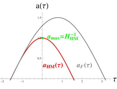
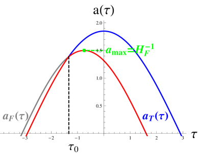
Figure 2: Illustration of scale factor $a(\tau)$ in cases of Hawking-Moss instanton (left panel) and Coleman-de Luccia instanton (right panel). In both cases, the evolution of the scale factor is labeled by red curves, while that of false vacuum $a_{\rm F}(\tau)$ and true vacuum $a_{\rm T}(\tau)$ are labeled by gray and blue curves, respectively. From the left panel, it is obvious that the maximum value of scale factor in HM case is different from that of false vacuum, which leads to a non-vanishing contribution to the tunneling rate as shown in Eq. (71). However, from the right panel, one finds that in the CDL case, the scale factor firstly evolves along that of true vacuum until some point $\tau_{0}$, then follows along that of false vacuum so that its maximum value coincides with that of false vacuum. Hence, using Eq. (69), contribution from the graviton mass vanishes in the CDL case.

V.3.1 Deviation from HM and thin-wall approximation

The HM instanton corresponds to a “thick-wall” limit where the curvature of local maximum of the potential is flat enough: ${\rm d}^{2}V(\sigma_{\rm HM})/{\rm d}\sigma^{2}=4H_{\rm HM}^{2}$. Using the perturbation approach in Sec. V.2, from Eq. (V.2), small deviation from HM instanton implies that

$$a_{\rm max}\simeq H_{\rm perturb}^{-1}\equiv\tilde{H}_{\rm HM}^{-1}\left(1+\frac{\varepsilon_{M}^{2}H_{\rm HM}^{2}}{8}\right)>a_{\rm HM}\,.$$ (72)

Inserting Eq. (72) into (V.3), the correction term for the perturbational approach around HM limit is evaluated as

$$B^{\rm mass}_{\rm perturb} =B^{\rm mass}(a_{\rm max}=H_{\rm perturb}^{-1})$$

$$=-\frac{4\pi^{2}m_{g}^{2}X_{\pm}Y_{\pm}}{3(FX_{\pm})^{4}}\left[\sqrt{1-\tilde{\alpha}^{2}}\left(2+\tilde{\alpha}^{2}\right)-\sqrt{1-\alpha_{\rm F}^{2}}\left(2+\alpha_{\rm F}^{2}\right)\right]+\frac{m_{g}^{2}\pi^{2}X_{\pm}Y_{\pm}{H}_{\rm HM}^{2}\varepsilon_{M}^{2}}{2\tilde{H}_{\rm HM}^{4}\sqrt{1-\tilde{\alpha}^{2}}}+\mathcal{O}(\varepsilon_{M}^{4})$$

$$=-\frac{4\pi^{2}m_{g}^{2}X_{\pm}Y_{\pm}}{3(FX_{\pm})^{4}}\left[\sqrt{1-\alpha_{\rm HM}^{2}}\left(2+\alpha_{\rm HM}^{2}\right)-\sqrt{1-\alpha_{\rm F}^{2}}\left(2+\alpha_{\rm F}^{2}\right)\right]+\frac{m_{g}^{2}\pi^{2}X_{\pm}Y_{\pm}\varepsilon_{M}^{2}}{3H_{\rm HM}^{4}\sqrt{1-\alpha_{\rm HM}^{2}}}$$

$$\quad+\mathcal{O}(\varepsilon_{M}^{4})\,.$$ (73)

Obviously, in the second step, the correction term of order $\varepsilon_{M}^{2}$ coincides with Eq. (65) as expected. Hence, the result in Sec. V.2 is recovered by applying Eq. (V.3).

For an intuitive analysis of deviation from thin-wall approximation, let us consider the classical trajectory of $-V(\sigma)$, where the scalar field is driven from the true vacuum $\sigma_{\rm T}$ toward the false vacuum $\sigma_{\rm F}$, as illustrated in Fig. 3. In the thin-wall limit, the friction term $3\mathcal{H}\sigma^{\prime}$ in Eq. (20) is neglected so that $\sigma$ can reach $\sigma_{\rm F}$ because of conservation of total energy. However, small deviation from the thin-wall limit implies a non-negligible friction term which causes loss of energy so that the scalar field starting from $\sigma_{\rm T}$ can only reach some point $\sigma_{\rm*}$ where $V(\sigma_{\rm*})>V(\sigma_{\rm F})$. Correspondingly, to calculate the maximum radius of the bubble, we have ${\rm d}a_{\rm*,max}/{\rm d}\tau=0$, then inserting into Eq. (19), one can evaluate in the following way:

$$a_{\rm*,max}=\sqrt{\frac{3}{V(\sigma_{\rm*})+\Lambda_{\pm}}}<a_{\rm{F,max}}\equiv H_{\rm F}^{-1}\,.$$ (74)

Figure 3: Illustration of classical trajectory with $-V(\sigma)$. When friction term $\mathcal{H}\sigma^{\prime}$ is taken into account, scalar field starting around $\sigma_{\rm T}$ along the potential cannot reach $\sigma_{\rm F}$ as in the thin-wall case. Instead, it will stop at some point $\sigma_{\rm*}$ and correspondingly gives the maximum radius $a_{\rm max}=a_{\rm*,max}<a_{\rm{F,max}}$ as shown in Eq. (74), hence leads to correction of tunneling rate arising from the non-vanishing graviton mass.

Again inserting Eq. (74) into (V.3), the correction term can be evaluated as:

$$B^{\rm mass}_{\rm*} =B^{\rm mass}(a_{\rm max}=H_{\rm*}^{-1})=\frac{4\pi^{2}m_{g}^{2}}{3}X_{\pm}Y_{\pm}\left[\frac{A(\alpha_{\rm*})}{H_{\rm*}^{4}}-\frac{A(\alpha_{\rm F})}{H_{\rm F}^{4}}\right]\neq 0\,.$$ (75)

Hence, small deviation from thin-wall limit makes $a_{\rm max}<a_{\rm{F,max}}$, which furthermore leads to corrections to the tunneling rate for the CDL instanton when compared to GR.

V.3.2 Beyond HM and thin-wall approximation

For a qualitative analysis, it is convenient to define a normalized function $\mathfrak{B}^{\rm mass}$ in the following way:

$$\mathfrak{B}^{\rm mass}(a_{\rm{max}}) \equiv-\frac{3(FX_{\pm})^{4}{B}^{\rm mass}}{4\pi^{2}m_{g}^{2}X_{\pm}Y_{\pm}}=\left[\sqrt{1-\left(FX_{\pm}a\right)^{2}}\left(2+\left(FX_{\pm}a\right)^{2}\right)\right]_{H_{\rm{F}}^{-1}}^{a_{\rm{max}}}$$

$$\equiv h(\alpha_{\rm max})-h(\alpha_{\rm F})\geq 0\,,$$ (76)

where we have defined the function $f$ and variable $\alpha$ as follows:

$$h(\alpha)\equiv\sqrt{1-\alpha^{2}}(2+\alpha^{2}),\qquad\alpha\equiv FX_{\rm\pm}a\,,$$ (77)

which is plotted in Fig. 4. It should be noted that $\alpha_{\rm F}\equiv FX_{\rm\pm}/H_{\rm F}$ coincides with the one in Ref. ZSS:2013 and leads to a constraint on the height of potential at false vacuum:

$$\alpha_{\rm F}\leq 1\quad\Longrightarrow\quad V(\sigma_{\rm F})\geq 3F^{2}X_{\pm}^{2}-\Lambda_{\pm}\,.$$ (78)

Inserting Eq. (V.3.2) into (69), the correction to the tunneling rate in dRGT massive gravity can be expressed as:

$$\Delta\Gamma\equiv\frac{\Gamma_{\rm MG}}{\Gamma_{\rm GR}}\simeq\exp(-B^{\rm mass})=\exp\left(\frac{4\pi^{2}m_{g}^{2}Y_{\pm}\mathfrak{B}^{\rm mass}}{3F^{4}X_{\pm}^{3}}\right)\,.$$ (79)

Provided with definite parameters $m_{g}^{2}$, $\alpha_{3}$ and $\alpha_{4}$, it is convenient to consider the behavior of $\mathfrak{B}^{\rm mass}$ with respect to $a_{\rm max}$, as plotted in Fig. 4. The values of normalized factor $\mathfrak{B}^{\rm mass}(a_{\rm max})$ defined in Eq. (V.3.2) are illustrated by black, blue and green double arrow lines, corresponding to the value in cases of HM (Sec. V.1), perturbations from HM (Sec. V.2) and deviation from thin-wall limit (Sec. V.3.1), respectively. In the thin-wall limit $a_{\rm max}=H_{\rm F}^{-1}$ (i.e. $\alpha=\alpha_{\rm F}$), hence the graviton mass has no contribution to the CDL tunneling rate as shown in Eq. (70). Provided with $Y_{\pm}>0$, under deviations from thin-wall limit, $a_{\rm max}=H_{\rm*}^{-1}<H_{\rm F}^{-1}$ (i.e. $\alpha=\alpha_{\rm*}$). Hence, a non-vanishing contribution to the CDL tunneling rate arises (as shown in the green double arrow line) and increases gradually, as evaluated in Eq. (75).

On the other hand, the most probable point is the HM limit which can be interpreted as “thick-wall” limit and correspondingly gives the largest tunneling rate as expected (black double arrow line). Perturbations around this limit give larger maximum radius $a_{\rm max}=H_{\rm perturb}^{-1}>H_{\rm HM}^{-1}$ (i.e. $\alpha=\alpha_{\rm perturb}$) as shown in Eq. (72), so the tunneling rate decreases monotonically (blue double arrow line). Thus, Eq. (V.3.2) implies monotonic behavior of function $\mathfrak{B}^{\rm mass}$ when $a_{\rm max}$ changes from $H_{\rm HM}^{-1}$ to $H_{\rm F}^{-1}$. Correspondingly, a monotonic behavior of the CDL tunneling rate with respect to different $a_{\rm max}$ is expected.

It should be noted that if $Y_{\pm}<0$, the above conclusion holds inversely, while $Y_{\pm}=0$ implies vanishing contribution to the tunneling rate. Since $0<\alpha\leq 1$, the value of $\mathfrak{B}^{\rm mass}$ is of order unity: $0\leq\mathfrak{B}^{\rm mass}<2$.

Moreover, when $F\longrightarrow 0$, the fiducial metric becomes Minkowskian. In this case, Eq. (79) reduces to the following form

$$\Delta\Gamma=\exp\left[\pi^{2}X_{\pm}Y_{\pm}m_{g}^{2}\left(H_{\rm F}^{-4}-a_{\rm max}^{4}\right)\right]\,.$$ (80)

Similarly as the behavior in de Sitter fiducial metric case as shown in Eq. (79), when $Y_{\pm}>0$, contribution to the CDL tunneling rate arising from the graviton mass appears when one go beyond “thin-wall” approximation, and increases monotonically until its maximum value at HM point. If $Y_{\pm}<0$, the conclusion holds inversely.

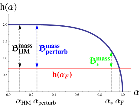
Figure 4: Plot of function $h(\alpha)$ defined in Eq. (77). For a given model, $\alpha_{\rm HM}$ and $\alpha_{\rm F}$ are definite, from which one obtains $h(\alpha_{\rm HM})$ and $h(\alpha_{\rm F})$. Using Eq. (V.3.2), the value of normalized factor $\mathfrak{B}^{\rm mass}(a_{\rm max})$ is illustrated by black, blue and green double arrow lines, corresponding to the value in cases of HM (Sec. V.1), perturbations from HM (Sec. V.2) and deviation from thin-wall limit (Sec. V.3.1), respectively. It should be noted that since $\alpha\in(0,1]$, the value of $\mathfrak{B}^{\rm mass}$ is of order unity: $\mathfrak{B}^{\rm mass}\in[0,2)$.

VI CDL v.s. HM process

In the previous section, it is found that when compared to the situation in GR, correction to the CDL tunneling rate will appear because of the non-vanishing graviton mass, and its value will change monotonically with respect of $a_{\rm max}$ until HM solution, i.e. from “thin-wall” to “thick-wall” case. Correspondingly, the physical picture of the analysis is that the shape of the potential changes gradually: the rate of its typical height of the local maximum to its width decreases monotonically.

On the other hand, it is interesting to consider another prospect: provided with the same shape of potential which satisfies the “thin-wall” condition Eq. (45), whether CDL instanton will dominate over HM one or inversely, which may imply sharp difference from GR where the CDL one always dominates if it exists. The comparison of the probability of the CDL process to that of HM is expressed as follows (for details of deduction see Appendix B):

$$\ln\left(\frac{P_{\rm CDL}}{P_{\rm HM}}\right)\approx 4\pi^{2}\left[\frac{16M_{\rm{Pl}}^{6}}{\Sigma^{2}}-\frac{m_{g}^{2}M_{\rm Pl}^{2}X_{\pm}Y_{\pm}}{3}\left(\frac{A(\alpha_{\rm F})}{H_{\rm F}^{4}}-\frac{A(\alpha_{\rm HM})}{H_{\rm HM}^{4}}\right)\right]\,,$$ (81)

assumming $\Lambda_{\pm,\rm T}=0$ and $\Lambda_{\pm,\rm F}=\epsilon M_{\rm Pl}^{4}$ with $\epsilon\ll 1$, where $A(\alpha)$ is defined in Eq. (58). In the context of GR where $m_{g}=0$, under the thin-wall approximation, the probability of the CDL instanton always dominates over the HM one. However, in dRGT massive gravity theory, there appears a term which is proportional to the mass of graviton, hence gives rise to the possibility that HM process may dominate over the CDL one when $Y_{\pm}>0$. It should be noted that, even when $F\to 0$, where the fiducial metric reduces to Minkowskian one, the function $A(\alpha)$ is finite, $\lim_{\alpha\to 0}A(\alpha)=3/4$, and then the ratio (81) is non-singular as has been stated in Ref. ZSS:2013 .

To find such a case, we note that within the range $\alpha\in(0,1]$, the function $A(\alpha)$ of order unity. Moreover, the thin-wall approximation implies that $H_{\rm F}^{-4}=9/(\epsilon^{2}M_{\rm Pl}^{4})\gg H_{\rm HM}^{-4}$. Hence, provided that the parameters $\alpha_{3}\sim\alpha_{4}\sim\mathcal{O}(1)$, one finds the condition on the value of graviton mass for HM process dominance:

$$m_{g}>\mathcal{O}\left(M_{\rm{Pl}}^{2}H_{\rm F}^{2}\Sigma^{-1}\right)\sim\mathcal{O}\left(a_{0}^{-1}\right)\,,$$ (82)

where $a_{0}$ is the radius of bubble defined in Eq. (49) while Eq. (98) has been used in the last step.

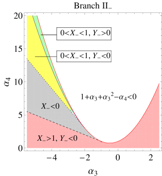
Figure 5: The sign of $Y_{\pm}$ is shown for Branch II₊ (left panel) and Branch II_- (right panel) solutions, respectively. The white region corresponds to $1+\alpha_{3}+\alpha_{3}^{2}-\alpha_{4}<0$ while in the gray one $X_{\pm}<0$, both of which should be excluded since the cosmological solution does not exist in these regions Gumrukcuoglu:2011open ; Gumrukcuoglu:2011perturb . In pink region, $X_{\pm}>1$ and $Y_{\pm}<0$, while green region corresponds to $1>X_{\pm}>0$ with $Y_{\pm}>0$. In blue region, $X_{+}>1$ and $Y_{+}>0$, while yellow region corresponds to $1>X_{-}>0$ and $Y_{-}>0$. Along the solid lines (defining the boundary between blue and pink regions for II₊, while the boundary between pink and yellow regions for II_-), $Y_{\pm}=0$ so that it reduces to the case in GR. The dotted lines denote $X_{\pm}=0$ where the solution ceases to exist. Along the dashed lines, $X_{\pm}$ diverges and thus defines another boundary of the solution space.

In order to see the possibilities for $Y_{\pm}>0$, in Fig. 5, we show the sign of $Y_{\pm}$ in the parameter space $(\alpha_{3},\alpha_{4})$ for Branch II₊ (left panel) and Branch II_- (right panel) solutions, respectively. The value of parameter $X_{\pm}$ is further constrained by the mass of tensor mode for self-accelerating solutions  Gumrukcuoglu:2011perturb

$$M_{\rm{GW}}^{2}=\left\{\begin{aligned} &m_{g}^{2}X_{+}(1-X_{+})\sqrt{1+\alpha_{3}+\alpha_{3}^{2}-\alpha_{4}}~{},\quad{\rm for}~{}~{}X_{+}\\ &m_{g}^{2}X_{-}(X_{-}-1)\sqrt{1+\alpha_{3}+\alpha_{3}^{2}-\alpha_{4}}~{},\quad{\rm for}~{}~{}X_{-}\end{aligned}\right.$$ (83)

which implies the constraints on parameter $X_{\pm}$ to avoid the tachyonic instability: in Branch II₊, $0<X_{+}<1$ and in Branch II_-, $X_{-}>1$. Hence, as shown in Fig. 5, there exists a region for $Y_{+}>0$ within the constraints (the green region in Branch II₊) while in Branch II_-, under the constraint $X_{-}>1$, the parameter $Y_{-}$ is always negative.

Hence, in Branch II₊, there exists the case where HM process would dominate over the CDL one, provided with Eq. (82). However, in Branch II_-, the CDL process always dominates. Moreover, it should be noted that in the limit where $\alpha_{3}=\alpha_{4}=0$, $X_{+}$ diverges so that only Branch II_- solution exists ZSS:2013 .

Thus, under the thin-wall approximation where the potential is very “sharp” at its local maximum, when the value of graviton mass is large enough so that Eq. (82) is satisfied, the HM process may dominate over the CDL one, which is very different from the case of GR. So we conclude that in the context of dRGT massive gravity theory, not only the shape of the potential, but also the values of parameters $\alpha_{3}$, $\alpha_{4}$ and $m_{g}$ will influence the tunneling process.

VII Conclusions

Towards the understanding of stability of vacuum in the landscape of vacua in dRGT massive gravity, in this paper, we investigated the Coleman-DeLuccia (CDL) solution, under the assumption that a tunneling field minimally couples to gravity. For comparison with Hawking-Moss (HM) instanton ZSS:2013 , we choose Branch-II_± for analysis and evaluate the corresponding tunneling rate of the CDL instanton. Firstly, we used the “thin-wall” approximation Coleman:1980 and found that the non-vanishing graviton mass term does not contribute to the tunneling rate.

To compare this result with the HM case, where the non-vanishing correction arises ZSS:2013 , we derived the CDL solution as perturbations around the HM case, which corresponds to a “thick-wall” approximation (or equivalently, the potential is very “flat” around its local maximum). In this approach, we found non-vanishing second-order perturbation to the tunneling rate due to the non-vanishing graviton mass, as shown in Eq. (65), which implies correction to the tunneling rate for the CDL instanton. Moreover, it is found that in this approach, when the parameter $Y_{\pm}>0$ (defined in Eq. (30)), HM process will dominate over the CDL one even when the CDL solutions exist.

In order to go beyond the thin-wall and thick-wall approximations, we rewrite the corrections to the tunneling rate due to the graviton mass in terms of $a_{\rm max}$, which is the largest radius of the bubble in Euclidean time (Eqs. (V.3)–(69)). It is found that in the thin-wall approximation, $a_{\rm max}$ coincides with the scale factor for the false vacuum, hence the contributions from the graviton mass cancel with the counter term of the false vacuum. Corrections to the CDL tunneling rate appear when one considers the deviations from thin-wall approximation, and its value varies monotonically with respect to $a_{\rm max}$ until the HM case, as illustrated in Fig. 4.

Moreover, provided with the same shape of potential which satisfies the condition for the thin-wall approximation, we compare the probabilities for the HM and CDL process. It is found that if the typical value for the graviton mass is larger than the inverse of bubble radius, the HM process may dominate over the CDL one, which is very different from the situation in GR. Hence, in dRGT massive gravity theory, not only the shape of the potential but also the value of the parameters $\alpha_{3}$, $\alpha_{4}$ and $m_{g}$ will qualitatively influence the tunneling process.

On the other hand, it is known that dRGT massive gravity theory suffers from some problems DeFelice:2012mx ; Acausality ; Acausality1 . Hence, as one step towards a more realistic model, it is necessary to study the tunneling issues in the extended massive gravity theories: for example, quasi-dilaton massive gravity DeFelice:2013 ; Quasidilaton:2013 ; Quasidilaton:2013perturb ; GHLMT ; FM:2013a ; FGM:2013 , varying-mass massive gravity Huang:2012 ; Huang:2013 ; Saridakis:2012 ; LSS:2013 ; HST:2013 ; WPC:2013 ; BHNMS:2013 or $SO(3)$ massive gravity lin:2013a ; lin:2013b . Especially, in the varying-mass massive gravity theory, due to the mass dependence, the effective cosmological constant $\Lambda_{\pm}$ of some vacuum may become larger even with a relatively smaller potential energy, which may imply a scenario of tunneling from a lower potential energy to a higher one. Investigations of the corresponding tunneling process is one of the future studies.

Appendix A Calculation of perturbations of action around HM solution

In this appendix, we present detailed calculations of perturbations in Euclidean action around HM solutions. It is obvious that from in Eq. (63), provided with Eq. (V.2), for our calculation of the perturbations of the action up to 2nd order, we should firstly consider the perturbations in the term $\sqrt{-(f^{\prime})^{2}}$. Under perturbation $f\longrightarrow f_{0}+\delta f$, we have:

$$\sqrt{-(f^{\prime})^{2}}=\sqrt{-(f_{0}^{\prime})^{2}}~{}\left|1+\frac{(\delta f)^{\prime}}{f_{0}^{\prime}}\right|$$ (84)

The constraint Eq. (18) implies the relationship $\delta f=X_{\pm}\delta a/b_{,f}$, so we have

$$(\delta f)^{\prime}=\frac{X_{\pm}}{b_{,f}}(\delta a)^{\prime}-\frac{X_{\pm}}{b_{,f}^{2}}\left(b_{,f}\right)^{\prime}\delta a\,,$$ (85)

while

$$b^{\prime}_{0}=b_{,f}f_{0}^{\prime}=X_{\pm}a_{0}^{\prime}\quad\Longrightarrow\quad f_{0}^{\prime}=\frac{X_{\pm}a_{0}^{\prime}}{b_{,f}}\,.$$ (86)

Combining these two equations, we then obtain the following relationship:

$$\frac{(\delta f)^{\prime}}{f_{0}^{\prime}}=\frac{1}{a_{0}^{\prime}}\left((\delta a)^{\prime}-\frac{\left(b_{,f}\right)^{\prime}}{b_{,f}}\delta a\right)\,.$$ (87)

On the other hand, noting that $b_{,f}=\pm\sqrt{\tilde{\alpha}^{2}\cos^{2}\left(\tilde{H}_{\rm HM}\tau\right)-1}$ with $\tilde{\alpha}\equiv FX_{\pm}/\tilde{H}_{\rm HM}$, we have:

$$\left(b_{,f}\right)^{\prime}=\pm\frac{-\tilde{\alpha}^{2}\tilde{H}_{\rm HM}\cos\left(\tilde{H}_{\rm HM}\tau\right)\sin\left(\tilde{H}_{\rm HM}\tau\right)}{\sqrt{\tilde{\alpha}^{2}\cos\left(\tilde{H}_{\rm HM}\tau\right)-1}}\,,$$ (88)

from which one immediately obtains that

$$\frac{\left(b_{,f}\right)^{\prime}}{b_{,f}}=\frac{\tilde{\alpha}^{2}\tilde{H}_{\rm HM}\cos\left(\tilde{H}_{\rm HM}\tau\right)\sin\left(\tilde{H}_{\rm HM}\tau\right)}{1-\tilde{\alpha}^{2}\cos^{2}\left(\tilde{H}_{\rm HM}\tau\right)}\,.$$ (89)

Inserting Eqs. (V.2) and (89) into Eq. (87), we obtain the following expression:

$$\frac{(\delta f)^{\prime}}{f_{0}^{\prime}}=\frac{\varepsilon_{M}^{2}{H}_{\rm HM}^{2}\cos^{2}\left(\tilde{H}_{\rm HM}\tau\right)}{8}\left(3+\frac{\tilde{\alpha}^{2}\cos^{2}\left(\tilde{H}_{\rm HM}\tau\right)}{1-\tilde{\alpha}^{2}\cos^{2}\left(\tilde{H}_{\rm HM}\tau\right)}\right)>0\,.$$ (90)

Hence, from Eqs. (84) and (90), we conclude that at range $\tilde{H}_{\rm HM}\tau\in(0,\pi/2)$, the the second order perturbation arising from the term $\sqrt{-(f^{\prime})^{2}}$ can be expressed in the following way:

$$\delta\sqrt{-(f^{\prime})^{2}}=\sqrt{-(f_{0}^{\prime})^{2}}~{}\frac{(\delta f)^{\prime}}{f_{0}^{\prime}}=\frac{\varepsilon_{M}^{2}X_{\pm}\tilde{H}_{\rm HM}^{2}\sin\left(\tilde{H}_{\rm HM}\tau\right)\cos^{2}\left(\tilde{H}_{\rm HM}\tau\right)}{8\sqrt{1-\tilde{\alpha}^{2}\cos^{2}\left(\tilde{H}_{\rm HM}\tau\right)}}\left[3+\frac{\tilde{\alpha}^{2}\cos^{2}\left(\tilde{H}_{\rm HM}\tau\right)}{1-\tilde{\alpha}^{2}\cos^{2}\left(\tilde{H}_{\rm HM}\tau\right)}\right]\,.$$ (91)

Now let us calculate the two parts in Eq. (63) separately. The first part reads

$$3\int_{0}^{\pi/2\tilde{H}_{\rm HM}}{\rm d}\tau~{}a_{\rm HM}^{2}\sqrt{-(f^{\prime})^{2}}\delta a = \frac{3}{\tilde{H}_{\rm HM}^{2}}\int_{0}^{\pi/2\tilde{H}_{\rm HM}}{\rm d}\tau~{}\cos^{2}\left(\tilde{H}_{\rm HM}\tau\right)\frac{X_{\pm}\sin\left(\tilde{H}_{\rm HM}\tau\right)}{\sqrt{1-\tilde{\alpha}^{2}\cos^{2}\left(\tilde{H}_{\rm HM}\tau\right)}}\frac{\varepsilon_{M}^{2}H_{\rm HM}^{2}}{8\tilde{H}_{\rm HM}}\cos^{3}\left(\tilde{H}_{\rm HM}\tau\right)$$ (92)

$$= \frac{3\varepsilon_{M}^{2}H_{\rm HM}^{2}X_{\pm}}{8\tilde{H}_{\rm HM}^{4}}\int_{0}^{\pi/2}{\rm d}z~{}\cos^{5}\left(z\right)\frac{\sin\left(z\right)}{\sqrt{1-\tilde{\alpha}^{2}\cos^{2}\left(z\right)}}$$

$$= -\frac{3\varepsilon_{M}^{2}H_{\rm HM}^{2}X_{\pm}}{8\tilde{H}_{\rm HM}^{4}}\int_{1}^{0}{\rm d}s~{}\frac{s^{5}}{\sqrt{1-\tilde{\alpha}^{2}s^{2}}}$$

$$= -\frac{3\varepsilon_{M}^{2}H_{\rm HM}^{2}X_{\pm}}{8\tilde{H}_{\rm HM}^{4}}\left[\frac{-8+\sqrt{1-\tilde{\alpha}^{2}}\left(8+4\tilde{\alpha}^{2}+3\tilde{\alpha}^{4}\right)}{15\tilde{\alpha}^{6}}\right]\,,$$

where in the second step, $z=\tilde{H}_{\rm HM}\tau$, and in the third step, $s=\cos(z)$. Meanwhile, the second part of Eq. (63) can be calculated by using Eq. (91) as follows:

$$\int_{0}^{\pi/2\tilde{H}_{\rm HM}}{\rm d}\tau~{}a_{\rm HM}^{3}\delta\sqrt{-(f^{\prime})^{2}} = \frac{\varepsilon_{M}^{2}{H}_{\rm HM}^{2}}{\tilde{H}_{\rm HM}^{3}}\int_{0}^{\pi/2\tilde{H}_{\rm HM}}{\rm d}\tau~{}\frac{X_{\pm}\sin\left(\tilde{H}_{\rm HM}\tau\right)\cos^{5}\left(\tilde{H}_{\rm HM}\tau\right)}{8\sqrt{1-\tilde{\alpha}^{2}\cos^{2}\left(\tilde{H}_{\rm HM}\tau\right)}}\left(3+\frac{\tilde{\alpha}^{2}\cos^{2}\left(\tilde{H}_{\rm HM}\tau\right)}{1-\tilde{\alpha}^{2}\cos^{2}\left(\tilde{H}_{\rm HM}\tau\right)}\right)$$ (93)

$$= \frac{\varepsilon_{M}^{2}X_{\pm}{H}_{\rm HM}^{2}}{\tilde{H}_{\rm HM}^{4}}\int_{0}^{\pi/2}{\rm d}z~{}\frac{\sin\left(z\right)\cos^{5}\left(z\right)}{8\sqrt{1-\tilde{\alpha}^{2}\cos^{2}\left(z\right)}}\left(3+\frac{\tilde{\alpha}^{2}\cos^{2}\left(z\right)}{1-\tilde{\alpha}^{2}\cos^{2}\left(z\right)}\right)$$

$$= -\frac{\varepsilon_{M}^{2}X_{\pm}{H}_{\rm HM}^{2}}{8\tilde{H}_{\rm HM}^{4}}\int_{1}^{0}{\rm d}s~{}\frac{s^{5}}{\sqrt{1-\tilde{\alpha}^{2}s^{2}}}\left(3+\frac{\tilde{\alpha}^{2}s^{2}}{1-\tilde{\alpha}^{2}s^{2}}\right)$$

$$= -\frac{\varepsilon_{M}^{2}X_{\pm}{H}_{\rm HM}^{2}}{8\tilde{H}_{\rm HM}^{4}}\frac{1}{5\tilde{\alpha}^{6}}\left(8+\frac{-8+4\tilde{\alpha}^{2}+\tilde{\alpha}^{4}-2\tilde{\alpha}^{6}}{\sqrt{1-\tilde{\alpha}^{2}}}\right)\,.$$

Thus, inserting Eqs. (92) and (93) into (63), one finally obtains the second order perturbation in Euclidean action:

$$\delta^{(2)}S=\frac{\pi^{2}m_{g}^{2}X_{\pm}Y_{\pm}{H}_{\rm HM}^{2}\varepsilon_{M}^{2}}{2\tilde{H}_{\rm HM}^{4}\sqrt{1-\tilde{\alpha}^{2}}}\,.$$ (94)

Appendix B Rate of the CDL process to HM one in thin-wall approximation

In this appendix, we derive Eq. (81) in details. For simplicity, let us assume $K=1$ and set the effective cosmological constant of the true vacuum $\Lambda_{\pm,\rm T}\equiv V(\sigma_{\rm T})+\Lambda_{\pm}=0$, while that of the false vacuum $\Lambda_{\pm,\rm F}\equiv V(\sigma_{\rm F})+\Lambda_{\pm}=\epsilon M_{\rm Pl}^{4}\ll M_{\rm Pl}^{4}$. Then from Eq. (47), one obtains:

$$B \simeq-2\pi^{2}\left\{6\int^{a_{0}}_{0}a{\rm d}a\left[1-\sqrt{K-(aH_{\rm F})^{2}}\right]-a^{3}_{0}\Sigma\right\}$$

$$=-12\pi^{2}\left\{\frac{a_{0}^{2}}{2}+\frac{1}{\epsilon}\left[\left(1-\frac{a_{0}^{2}}{3}\epsilon\right)^{\frac{3}{2}}-1\right]\right\}+2\pi^{2}a_{0}^{3}\Sigma\,,$$ (95)

which is stationary when

$$a_{0}=\frac{12\Sigma}{3\Sigma^{2}+4\epsilon}\,.$$ (96)

Inserting Eq. (96) into (B), one obtains:

$$B\simeq 12\pi^{2}\left[\frac{72\Sigma^{2}(\Sigma^{2}-4\epsilon)}{(3\Sigma^{2}+4\epsilon)^{3}}+\frac{1}{\epsilon}\left(1-\left|\frac{3\Sigma^{2}-4\epsilon}{3\Sigma^{2}+4\epsilon}\right|^{3}\right)\right]\,.$$ (97)

In order to evaluate the absolute value term in the right-hand side of Eq. (97), we note that from Eq. (49), the extreme value for tension $\Sigma$ can be also evaluated as follows:

$$\Sigma=\frac{2}{a_{0}}\left(1-\sqrt{1-\frac{a_{0}^{2}\epsilon}{3}}\right)\approx\frac{a_{0}\epsilon}{3}\,.$$ (98)

Since $a_{0}<H_{\rm F}^{-1}=\sqrt{3/\epsilon}$, Eq. (98) implies that $3\Sigma^{2}-4\epsilon<-3\epsilon<0$. Thus, from Eq. (97), we finally obtain that:

$$B \simeq 12\pi^{2}\left\{\frac{72\Sigma^{2}(\Sigma^{2}-4\epsilon)}{(3\Sigma^{2}+4\epsilon)^{3}}+\frac{1}{\epsilon}\left[1+\left(\frac{3\Sigma^{2}-4\epsilon}{3\Sigma^{2}+4\epsilon}\right)^{3}\right]\right\}$$

$$=\frac{24\pi^{2}}{\epsilon}\left(1+\frac{4\epsilon}{3\Sigma^{2}}\right)^{-2}\,.$$ (99)

Hence, the corresponding tunneling rate defined in Eq. (6) is expressed as:

$$P_{\rm thin-wall}\approx\exp\left[-\frac{24\pi^{2}}{\epsilon}\left(1+\frac{4\epsilon}{3\Sigma^{2}}\right)^{-2}\right]\approx\exp\left(-\frac{24\pi^{2}}{\epsilon}+\frac{64\pi^{2}}{\Sigma^{2}}\right)\,,$$ (100)

while by using Eqs. (V.3.2) and (79), that of thick-wall approximation can be expressed as kklt

$$P_{\rm thick-wall} \approx\exp\left[-\frac{24\pi^{2}}{\epsilon}\left(1-\frac{\epsilon}{\Lambda_{\pm,\rm eff}}\right)+\frac{4\pi^{2}m_{g}^{2}Y_{\pm}\mathfrak{B}^{\rm mass}}{3F^{4}X_{\pm}^{3}}\right]$$

$$\approx\exp\left(-\frac{24\pi^{2}}{\epsilon}+\frac{24\pi^{2}}{\Lambda_{\pm,\rm eff}}+\frac{4\pi^{2}m_{g}^{2}Y_{\pm}\mathfrak{B}^{\rm mass}}{3F^{4}X_{\pm}^{3}}\right)\,.$$ (101)

Combining Eqs. (100) and (B), one can compare the probability of the CDL process to that of HM as follows:

$$\ln\left(\frac{P_{\rm CDL}}{P_{\rm HM}}\right)=4\pi^{2}\left(\frac{16}{\Sigma^{2}}-\frac{6}{\Lambda_{\pm,\rm eff}}-\frac{m_{g}^{2}Y_{\pm}\mathfrak{B}^{\rm mass}(a_{\rm max}=H^{-1}_{\rm HM})}{3F^{4}X_{\pm}^{3}}\right)\,.$$ (102)

Noting that from Eq. (48), one can make a comparison between $\Sigma^{2}$ and $\Lambda_{\pm,\rm eff}$ as follows (here $M_{\rm Pl}$ is recovered for comparison)

$$\frac{\Sigma}{M_{\rm Pl}\sqrt{\Lambda_{\pm,\rm eff}}} \sim\frac{\int_{\sigma_{\rm T}}^{\sigma_{\rm F}}{\rm d}\sigma\sqrt{V(\sigma)-V(\sigma_{\rm T})}}{M_{\rm Pl}H_{\rm HM}}<\frac{\sqrt{V(\sigma_{\rm HM})-V(\sigma_{\rm T})}}{M_{\rm Pl}H_{\rm HM}}\Delta\sigma$$

$$=\frac{\sqrt{V(\sigma_{\rm HM})+\Lambda_{\pm}}}{M_{\rm Pl}H_{\rm HM}}\Delta\sigma=\frac{\Delta\sigma}{M_{\rm Pl}}\sim\frac{\big{|}\sigma_{\rm HM}-\sigma_{\rm T}\big{|}}{M_{\rm Pl}}\,,$$ (103)

where $\Delta\sigma\equiv|\sigma_{\rm F}-\sigma_{\rm T}|$ and we have used $V(\sigma_{\rm T})=-\Lambda_{\pm}$. On the other hand, expending the potential near $\sigma_{\rm HM}$, we have

$$V(\sigma)=V(\sigma_{\rm HM})-\frac{M^{2}}{2}(\sigma-\sigma_{\rm HM})^{2}+...\,,$$ (104)

where $M^{2}\equiv-{\rm d}^{2}V(\sigma)/{\rm d}\sigma^{2}|_{\sigma=\sigma_{\rm HM}}$. So one obtains

$$\frac{M^{2}}{2}(\sigma_{\rm T}-\sigma_{\rm HM})^{2}\approx V(\sigma_{\rm HM})-V(\sigma_{\rm T})<H_{\rm HM}^{2}\quad\Longrightarrow\quad\big{|}\sigma_{\rm T}-\sigma_{\rm HM}\big{|}<\frac{H_{\rm HM}}{M}\,.$$ (105)

Inserting this into Eq.(104), we find that

$$\frac{\Sigma}{M_{\rm Pl}\sqrt{\Lambda_{\pm,\rm eff}}}<\frac{H_{\rm HM}}{M}\,.$$ (106)

In the thin-wall approximation, the typical height of the local maximum of the potential is much larger than its width so that $M^{2}\gg H_{\rm HM}^{2}$, then one obtains that

$$\Sigma^{2}\ll M_{\rm Pl}^{2}\Lambda_{\pm,\rm eff}\,.$$ (107)

We note that Eq. (107) can be justified in another way: from Eq. (49), using the relationship $H_{\rm F}^{2}-H_{\rm T}^{2}=\epsilon/3$, the radius of the bubble can be expressed as Coleman:1980

$$a_{0}=\frac{4\Sigma}{\sqrt{\left(\Sigma^{2}+\frac{4\epsilon}{3}\right)^{2}+16\Sigma^{2}H_{\rm T}^{2}}}=\frac{12\Sigma}{3\Sigma^{2}+4\epsilon}\sim\frac{1}{\Sigma}\,,$$ (108)

where we have used the assumption $H_{\rm T}^{2}\equiv\Lambda_{\pm,\rm T}/3=0$ and $\Sigma^{2}\gtrsim\mathcal{O}(\epsilon)$. On the other hand, using Eqs. (37) and (41), one finds that

$$a^{\prime}=\sqrt{1-a^{2}H_{\rm T}^{2}}=1\,,$$ (109)

so using the relationship ${\rm d}\sigma=\sigma^{\prime}{\rm d}a/a^{\prime}$, the thickness of the wall can be approximately evaluated as

$$\Delta a=\frac{a^{\prime}\Delta\sigma}{\sigma^{\prime}}\approx\frac{\Sigma}{V(\sigma_{\rm HM})-V(\sigma_{\rm T})}=\frac{\Sigma}{\Lambda_{\pm,\rm eff}}\,,$$ (110)

where $\Delta\sigma\equiv|\sigma_{\rm F}-\sigma_{\rm T}|\approx\Sigma/\sqrt{V-V(\sigma_{\rm T})}$. The thin-wall approximation is valid if $a_{0}/\Delta a\gg 1$, so one obtains $\Sigma^{2}\ll\Lambda_{\pm,\rm eff}$ kklt , which verifies Eq. (107). Thus, in the thin-wall approximation, Eq. (102) reduces to the following form:

$$\ln\left(\frac{P_{\rm CDL}}{P_{\rm HM}}\right) \approx 4\pi^{2}\left(\frac{16}{\Sigma^{2}}-\frac{m_{g}^{2}Y_{\pm}\mathfrak{B}^{\rm mass}(a_{\rm max}=H^{-1}_{\rm HM})}{3F^{4}X_{\pm}^{3}}\right)$$

$$=4\pi^{2}\left[\frac{16}{\Sigma^{2}}-\frac{m_{g}^{2}X_{\pm}Y_{\pm}}{3}\left(\frac{A(\alpha_{\rm F})}{H_{\rm F}^{4}}-\frac{A(\alpha_{\rm HM})}{H_{\rm HM}^{4}}\right)\right]\,,$$ (111)

where we used the Eq. (58) for definition of function $A(\alpha)$. In the context of GR where $m_{g}=0$, provided that the CDL instantons exist, the CDL process always dominates over the HM one kklt .

References

• (1) M. Fierz and W. Pauli, Proc. Roy. Soc. Lond. A 173, 211-232 (1939).
• (2) D. G. Boulware and S. Deser, Phys. Rev. D 6, 3368-3382 (1972).
• (3) P. Creminelli, A. Nicolis, M. Papucci and E. Trincherini, JHEP 0509, 003 (2005) [hep-th/0505147].
• (4) V. A. Rubakov and P. G. Tinyakov, Phys. Usp. 51, 759-792 (2008). [arXiv:0802.4379 [hep-th]].
• (5) K. Hinterbichler, Rev. Mod. Phys. 84, 671-710 (2012). [arXiv:1105.3735 [hep-th]].
• (6) C. de Rham and G. Gabadadze, Phys. Rev. D 82, 044020 (2010). [arXiv:1007.0443 [hep-th]].
• (7) C. de Rham, G. Gabadadze and A. J. Tolley, Phys. Rev. Lett.  106, 231101 (2011). [arXiv:1011.1232 [hep-th]].
• (8) S. F. Hassan and R. A. Rosen, JHEP 1107, 009 (2011) [arXiv:1103.6055 [hep-th]].
• (9) S. F. Hassan and R. A. Rosen, Phys. Rev. Lett. 108, 041101 (2012) [arXiv:1106.3344 [hep-th]].
• (10) S. F. Hassan, R. A. Rosen and A. Schmidt-May, JHEP 1202, 026 (2012) [arXiv:1109.3230 [hep-th]].
• (11) G. D’Amico, C. de Rham, S. Dubovsky, G. Gabadadze, D. Pirtskhalava and A. J. Tolley, Phys. Rev. D 84, 124046 (2011) [arXiv:1108.5231 [hep-th]].
• (12) A. E. Gümrükçüoğlu, C. Lin and S. Mukohyama, JCAP  11, 030 (2011). [arXiv:1109.3845 [hep-th]].
• (13) T. Kobayashi, M. Siino, M. Yamaguchi and D. Yoshida, Phys. Rev. D 86, 061505 (2012) [arXiv:1205.4938 [hep-th]].
• (14) P. Gratia, W. Hu and M. Wyman, Phys. Rev. D 86, 061504 (2012) [arXiv:1205.4241 [hep-th]].
• (15) S. Weinberg, Rev. Mod. Phys.  61, 1 (1989).
• (16) S. Nobbenhuis, Found. Phys.  36, 613 (2006) [gr-qc/0411093].
• (17) L. Susskind, In *Carr, Bernard (ed.): Universe or multiverse?* 247-266 [hep-th/0302219].
• (18) S. W. Hawking and I. G. Moss, Phys. Lett. B 110, 35 (1982).
• (19) Y. Zhang, R. Saito and M. Sasaki, JCAP 1302, 029 (2013). [arXiv:1210.6224 [hep-th]].
• (20) J. B. Hartle and S. W. Hawking, Phys. Rev. D 28, 2960 (1983).
• (21) M. Sasaki, D. Yeom and Y. Zhang, Class. Quant. Grav. 30, 232001 (2013) [arXiv:1307.5948 [gr-qc]].
• (22) S. R. Coleman and F. De Luccia, Phys. Rev. D 21, 3305 (1980).
• (23) P. Batra and M. Kleban, Phys. Rev. D 76, 103510 (2007), [hep-th/0612083].
• (24) S. R. Coleman, V. Glaser and A. Martin, Commun. Math. Phys.  58, 211 (1978).
• (25) B-H. Lee and W. Lee, Class. Quant. Grav. 26, 225002 (2009), [arXiv:0809.4907 [hep-th]].
• (26) B-H. Lee, C. H. Lee, W. Lee and C. Oh, Phys. Rev. D 82, 024019 (2010), [arXiv:0910.1653 [hep-th]].
• (27) B-H. Lee, C. H. Lee , W. Lee and C. Oh, Phys. Rev. D 85, 024022 (2012), [arXiv:1106.5865 [hep-th]].
• (28) B-H. Lee, C. H. Lee , W. Lee and C. Oh, arXiv:1311.4279 [hep-th].
• (29) S. F. Hassan and R. A. Rosen, JHEP 1202, 126 (2012) [arXiv:1109.3515 [hep-th]].
• (30) M. S. Volkov, JHEP 1201, 035 (2012) [arXiv:1110.6153 [hep-th]].
• (31) D. Comelli, M. Crisostomi, F. Nesti and L. Pilo, JHEP 1203, 067 (2012) [Erratum-ibid.  1206, 020 (2012)] [arXiv:1111.1983 [hep-th]].
• (32) D. Langlois and A. Naruko, Class. Quant. Grav. 29, 202001 (2012). [arXiv:1206.6810 [hep-th]].
• (33) C. de Rham and S. Renaux-Petel, JCAP 1301, 035 (2013) [arXiv:1206.3482 [hep-th]];
• (34) T. Tanaka and M. Sasaki, Prog. Theor. Phys.  88, 503 (1992)
• (35) A. E. Gümrükçüoğlu, C. Lin and S. Mukohyama, JCAP  03, 006 (2012). [arXiv:1111.4107 [hep-th]].
• (36) S. Deser and A. Waldron, Phys. Rev. Lett. 110, 111101 (2013) [arXiv:1212.5835 [hep-th]].
• (37) S. Deser, K. Izumi, Y. C. Ong and A. Waldron, Phys. Lett. B 726, 544 (2013) [arXiv:1306.5457 [hep-th]].
• (38) A. De Felice, A. E. Gümrükçüoğlu and S. Mukohyama, Phys. Rev. Lett. 109, 171101 (2012) [arXiv:1206.2080 [hep-th]].
• (39) G. D’Amico, G. Gabadadze, L. Hui and D. Pirtskhalava, Phys. Rev. D 87, (2013) 064037. [arXiv:1206.4253 [hep-th]].
• (40) G. D’Amico, G. Gabadadze, L. Hui and D. Pirtskhalava, Class. Quant. Grav. 30 (2013) 184005 [arXiv:1304.0723 [hep-th]].
• (41) A. De Felice, A. E. Gümrükçüoğlu, C. Lin and S. Mukohyama, JCAP 1305, (2013) 035 [arXiv:1303.4154 [hep-th]].
• (42) A. E. Gümrükçüoğlu, K. Hinterbichler, C. Lin, S. Mukohyama and M. Trodden, Phys. Rev. D 88, 024023 (2013). [arXiv:1304.0449 [hep-th]].
• (43) A. De Felice and S. Mukohyama, arXiv:1306.5502 [hep-th].
• (44) A. De Felice, A. E. Gümrükçüoğlu and S. Mukohyama, arXiv:1309.3162 [hep-th].
• (45) Q. Huang, Y. Piao and S. Zhou, Phys. Rev. D 86, 124014 (2012) [arXiv:1206.5678 [hep-th]].
• (46) Q. Huang, K. Zhang and S. Zhou. JCAP 1308, 050 (2013) [arXiv:1306.4740 [hep-th]].
• (47) E. N. Saridakis, Class. Quant. Grav.30, 075003 (2013) [arXiv:1207.1800 [gr-qc]].
• (48) G. Leon, J. Saavedra and E. N. Saridakis, Class. Quant. Grav.30, 135001 (2013) [arXiv:1301.7419 [gr-qc]].
• (49) K. Hinterbichler, J. Stokes and M. Trodden, Phys. Lett. B 725, 1 (2013) [arXiv:1301.4993 [astro-ph]].
• (50) D. Wu, Y. Piao and Y. Cai, Phys. Lett. B 721, 7 (2013) [arXiv:1301.4326 [hep-th]].
• (51) K. Bamba, Md. Wali Hossain, S. Nojiri, R. Myrzakulov and M. Sami, arXiv:1309.6413 [hep-th].
• (52) C. Lin, arXiv:1305.2069 [hep-th].
• (53) C. Lin, arXiv:1307.2574 [hep-th].
• (54) S. Kachru, R. Kallosh, A. D. Linde and S. P. Trivedi, Phys. Rev. D 68, 046005 (2003) [hep-th/0301240].