Quantifying randomness in protein protein interaction networks of different species: A random matrix approach
Abstract
We analyze protein-protein interaction networks for six different species under the framework of random matrix theory. Nearest neighbor spacing distribution of the eigenvalues of adjacency matrices of the largest connected part of these networks emulate universal Gaussian orthogonal statistics of random matrix theory. We demonstrate that spectral rigidity, which quantifies long range correlations in eigenvalues, for all protein-protein interaction networks follow random matrix prediction up to certain ranges indicating randomness in interactions. After this range, deviation from the universality evinces underlying structural features in network.
keywords:
Random matrix theory, Protein Protein interaction networks, Spectra1 Introduction
Random matrix theory (RMT), proposed by Wigner to explain the statistical properties of nuclear spectra, has elucidated a remarkable success in understanding complex systems which include disordered systems, quantum chaotic systems, spectra of large complex atoms, etc. Recently complex networks have also been analyzed in RMT framework bringing them into the universality class of Gaussian orthogonal ensemble (GOE) [1, 2, 3, 4]. Systematic investigations performed on model networks establish correlation between their structural properties and spectral properties inspected by RMT. This paper validates the access of a mathematical tool, RMT, to study protein-protein interaction (PPI) networks of different species, as model systems, under RMT framework. By interaction we mean that a protein may change conformation of another protein leading to a change in its affinity for different groups or may lead to addition or removal of a group in the molecule. The interaction is highly specific i.e. it can discriminate among thousands of different molecules in its environment and selectively interact with one or two [5].
A network representation of PPI in addition to providing a better understanding of protein function, serves us with a powerful model of various functional pathways elucidating mechanics at cellular level [6, 7, 8]. Recently it has been realized that analysis of a network representation of such interactions, in comparison to pairwise analysis, provides a much better understanding of the processes occurring in biological systems [9, 10, 11, 12, 13]. These studies indicate a strong correlation between the interaction networks and expression properties of the proteins having similar expression dynamics i.e. they tend to form clusters of either static or dynamic proteins [14, 15]. Furthermore, analysis of PPI networks have contributed in various disease related biological studies, for instance study of human interaction data and Alzheimer’s disease proteins has enriched our knowledge about its protein targets [16]. Some of the PPI network studies reveal that pathogens tend to interact with hub proteins and proteins that are central to many paths in the network [17].
Analysis performed here involves construction of networks in such a way that any pair of proteins can achieve only two states i.e. either they are connected or not connected. We demonstrate that nearest neighbor spacing distribution (NNSD) of PPI networks of different species exhibit a similar statistical behavior of RMT, bringing them all under the same universality class. Furthermore, long range correlations in spectra display a wide range of behaviors.
2 RMT and Networks - What is the connection?
The random matrix approach regarded the Hamiltonian of a heavy nucleus (which is very complex due to the complexity of interactions between various nucleons) as behaving like a random matrix chosen from Gaussian orthogonal ensemble (GOE) having a probability density . Energy levels were approximated by the eigenvalues of this matrix and their statistics were studied [18]. The functional form of defines the type of ensemble. Later this theory was successfully applied in the study of spectra of different complex systems including disordered systems, quantum chaotic systems, spectra of large complex atoms etc [19]. RMT is also shown to be of great use while understanding the statistical structure of the empirical cross-correlation matrices appearing in the study of multivariate time series. The classical complex systems where RMT has been successfully applied are stock market [20]; brain [21]; patterns of atmospheric variability [22], physiology and DNA-binding proteins [23] etc. Our previous studies elucidate that different model networks, namely scale-free, small world, random networks and modular networks ensue universal GOE statistics of RMT.
A network is represented in the form of an adjacency matrix in which a corresponding element is set to 1 if node is connected with node and 0 otherwise. The set of eigenvalues of an adjacency matrix is called its spectrum. Spectrum of a network is related with its various topological properties [24]. Spectral density of adjacency matrix of a random network reflects a semicircular law [25], which interestingly is one of the properties of random matrix chosen from a Gaussian ensemble [18]. Even though the analysis of some real world networks and various model networks capturing real world properties manifest somewhat different spectral densities [25, 26], our previous studies reveal the universal GOE statistics of eigenvalue fluctuations of the above mentioned networks [1, 27, 28]. This similarity in the NNSD of spectra of a random matrix and that of different model networks furnishes more insight into the physical significance of spectra of networks. These eigenvalues can be treated as elements signifying different topological states of a network or it can be said that the spectra of a network gives us information about the property which is used to define the entries of adjacency matrix (connections) of network, as in case of nuclear spectra, different energy levels of nucleus are approximated by eigenvalues of a random matrix (representing Hamiltonian i.e. energy of system). One more aspect, which this connection between RMT and networks demonstrate, is the existence of some amount of randomness in these networks. We take our previous studies a step further and validate the applicability of RMT on PPI networks, demonstrating that they all come under the same universality class.
3 Data sources and network construction
To construct PPI networks of different species, first interaction data is downloaded from publicly available data source DIP (database of interacting proteins) [29]. DIP manages a database for experimentally determined protein interactions in all organisms. It integrates information from different sources to create a single set of protein protein interaction. Data from this source is widely used for various data analyses and biological studies [30]. In the database, each protein and each interaction is represented by a unique id, and for each interaction, information of interactors are given. With this information, an interaction network is constructed for a species. Here nodes of the network are represented by the proteins and a connection in the network corresponds to the interaction occurring between the two protein represented by two nodes. Next we detect largest connected cluster in these networks. Corresponding adjacency matrix has a entry if protein interacts with protein and 0 otherwise. PPI networks are undirected and so the adjacency matrix is symmetric entailing all real eigenvalues. In all the networks, a protein interaction with itself, if any, are ignored. Below we provide a brief description of different species studied here.
4 Method of Analysis
4.1 NNSD
In the following, we introduce spacing distribution of random matrices. Let eigenvalues of a network be denoted by and . In order to get universal properties of the fluctuations of eigenvalues, it is customary in RMT to unfold the eigenvalues by a transformation , where is average integrated eigenvalue density [18]. Since we do not have any analytical form for , we numerically unfold the spectrum by polynomial curve fitting (for elaborate discussion on unfolding, see Ref. [18]). After unfolding, average spacing becomes unity, independent of the system. Using the unfolded spectra, we calculate spacings as . In the case of GOE statistics, the nearest neighbor spacing distribution (NNSD) is denoted by
| (1) |
For intermediate cases, the spacing distribution is described by Brody parameter [31].
| (2a) | ||||
| where and are determined by the parameter as follows: | ||||
| (2b) | ||||
This is a semi-empirical formula characterized by parameter . As goes from 0 to 1, the Brody distribution smoothly changes from Poisson to GOE. We fit spacing distributions of different networks by the Brody distribution . This fitting gives an estimation of , and consequently identifies whether the spacing distribution of a given network is Poisson, GOE, or the intermediate of these two [31].
Apart from NNSD, the next nearest-neighbor spacing distribution (nNNSD) is also used to characterize the statistics of eigenvalue fluctuations. We calculate this distribution of next nearest-neighbor spacing,
| (3) |
between the unfolded eigenvalues. Factor of two at the denominator is inserted to make the average of next nearest- neighbor spacing unity. According to Ref. [18], the nNNSD of GOE matrices is identical to the NNSD of Gaussian symplectic ensemble (GSE) matrices, i.e.,
| (4) |
The NNSD and nNNSD reflect only local correlations among the eigenvalues. The spectral rigidity, measured by the -statistics of RMT, preserves information about the long-range correlations among eigenvalues and is a more sensitive test for studying RMT properties of the matrix under investigation. In the following, we describe the procedure to calculate this quantity.
4.2 statistics
The -statistics measures the least-square deviation of the spectral staircase function representing average integrated eigenvalue density from the best fitted straight line for a finite interval of length of the spectrum given by
| (5) |
where and are regression coefficients obtained after least square fit. Average over several choices of x gives the spectral rigidity . For GOE case, depends logarithmically on L, i.e.
| (6) |
5 Results
In this section we present various results obtained for each of the different PPI networks constructed. All the results are produced for the adjacency matrix corresponding to the largest connected cluster of each network. For completeness we briefly discuss degree distribution and density distribution for all these species, after which present random matrix results.
5.1 Degree Distribution
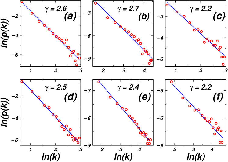
Fig. (1) plots degree distribution for each of the PPI networks for the six species studied and corresponding values are obtained. The results confirm that all the PPI networks are scale-free entailing power law [32].
5.2 Spectral Analysis
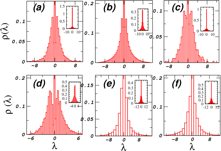
The PPI networks considered here are undirected entailing all real eigenvalues. The spacing between the adjacent smallest eigenvalues is very large which sharply decreases initially, then gradually falls to zero followed by a sharp increase. The plots do not provide a quantitative estimate that how similar eigenvalues are spaced together in different networks but more importantly it convey the information about degeneracy in the network which has to been taken into account for NNSD analysis. Real world networks, in general, are very sparse and are reported to have a large number of zero eigenvalues[33]. Fig. 2 plots normalized spectral density for each of the networks. Profile for the spectral density looks more like bell shaped for all the networks. Even though the global nature of variation of spectral density with the eigenvalues looks similar in different networks, minute observations of the plot in the inset of spectral density figures indicate that they vary differently in different networks.
5.3 Short range correlations in eigenvalues
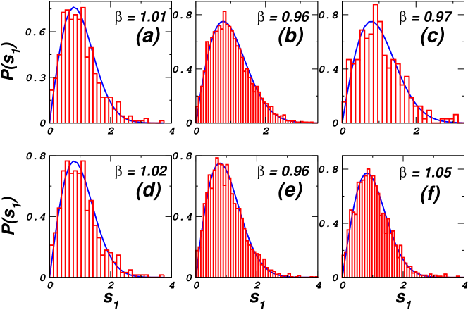
From the spectra of each of the networks we calculate the spacing distribution for adjacent eigenvalues. Negative and positive eigenvalues are unfolded separately with different polynomial functions. The degenerate eigenvalues, other than zero, are considered as a single eigenvalue. The flat region corresponding to zero eigenvalue is excluded from the analysis. Extreme eigenvalues at both the ends of the spectra are also not considered. Fig. 3 plots NNSD for different networks corresponding to different species. All the plots are fitted with the Brody distribution given by Eq.2.
The value of fitted Brody parameter indicates that the NNSD of eigenvalues for all the PPI networks ensue GOE distribution. This is not a trivial result and it renders a new look into such interaction networks, as in spite of genetic differences, differences in internal environment, biological activities, modes of functioning in those species affecting their protein-protein interactions, they exhibit a similar universal behavior predicted by RMT. Another RMT interpretation of GOE statistics suggests that some amount of randomness is present in PPI networks.
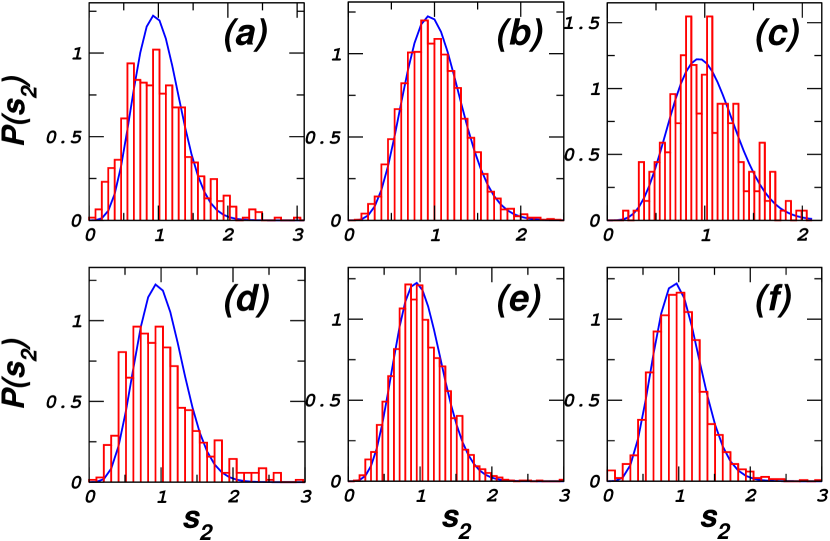
Same unfolded eigenvalues have been used to calculate next nearest-neighbor spacings as in Eq. 3. nNNSD for all PPI networks are plotted in Fig. 4. For C. elegans and H. sapiens, though NNSD emulates GOE statistics of RMT, nNNSD shows deviation from it, this supports that NNSD is not very sensitive test of RMT, and in order to learn more about correlations in eigenvalues one should go for other tests like nNNSD or statistics. For other networks, next nearest-neighbor spacings confirm random matrix predictions of GOE statistics.
5.4 Long range correlations in eigenvalues
| Species | N | L | % L/N | ||||
| C. elegans | 2646 | 2386 | 516 | 516 | 1354 | - | - |
| D. melanogaster | 7451 | 7321 | 2504 | 2506 | 2311 | 28 | 0.38 |
| H. pylori | 732 | 709 | 196 | 196 | 317 | 13 | 1.83 |
| H. sapiens | 3164 | 2138 | 628 | 646 | 864 | - | - |
| S. cerevisiae | 5080 | 5019 | 1995 | 2048 | 976 | 18 | 0.35 |
| E. coli | 2969 | 2209 | 851 | 871 | 487 | 9 | 0.41 |
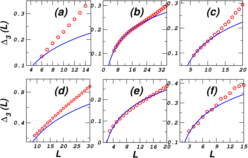
As explained in the introduction that NNSD and nNNSD offer insight into only short range correlations among the eigenvalues. To probe for long range correlations one employs statistics of the spectrum of a network. For all the networks, statistics is calculated using Eq. (5). Fig. (5) elucidates this statistics for various PPI networks, indicating that RMT does not provide a good model for PPI networks of C. elegans and H. sapiens. Whereas, other PPI networks conform with statistics of GOE up to a certain range , after which deviation from this universal GOE statistics occurs. According to RMT, eigenvalues are correlated up to this range. Different ranges of in different species, for which statistics imitates RMT, can be understood as different amount of randomness in corresponding PPI network [27]. Last column of the Table. 1 displays a qualitative measure of randomness in network as detected in eigenvalue correlations.
6 Summary of results for different species
C. elegans - The eigenvalues vary in the interval . Degeneracy in three regions is observed for =-1, 0 and 1. Out of the 2386 eigenvalues, nearly 56% of the eigenvalues are zero. Although the degeneracy at -1 and 1 is considerably less as compared to zero, of the eigenvalues are degenerate for each of =-1 and =1. The degree distribution for the corresponding network clearly reveals that it is scale-free with = 2.6. The normalized spectral density, on the other hand, shows a little deviation from the triangular distribution. Spectral density as expected is very large around 0 and decreases as the magnitude of eigenvalue increases. The universality of C. elegans PPI networks is quantified by the NNSD analysis. The quantifying factor is the Brody parameter which for this network comes out to be , but nNNSD and indicate deviations. There can be two interpretations of this behavior. First one is that PPI network of C. elegans cannot be modeled using GOE of RMT, as NNSD complying GOE statistics is not very sensitive or reliable test. Second interpretation is that there is a very minimal amount of randomness in underlying matrix bringing upon correlations between only nearest neighbors in spectra.
D. melanogaster - The eigenvalues vary in the interval . Out of the 7321 eigenvalues, 31% are 0, only 9 and 5 eigenvalues show degeneracy for =-1 and 1, respectively. Thus, the amount of degeneracy in this species is considerably less as compared to C. elegans and the plot for eigenvalues is smoother as well. This network also fits well with the power law degree distribution ( = 2.7), verifying the scale-free nature for this network as well. Normalized spectral density for this network also resembles the bell-shaped curve but the density as compared to that of C. elegans decreases much slower as the magnitude of eigenvalues increases. The NNSD fitting with the Brody Distribution gives , which clearly indicates the GOE behavior of NNSD. nNNSD too abides well with GOE predictions of RMT. Long range correlations measured by statistics agrees with RMT prediction up to .
H. pylori - The 709 eigenvalues vary between . Degeneracy, in this case, is observed only for =0, with of the eigenvalues being 0. Degree distribution found to obey power law verifying its class of scale-free networks. Corresponding value is 2.2. The normalized spectral density for network of this species is more triangular than the above two species. Brody fitting to NNSD yields . nNNSD agrees well with the NNSD of GSE matrices. Long range correlation ( statistics) ensues GOE statistics up to length .
H. sapiens - Network for H. sapiens exhibits three types of degeneracy. 40% of the 2138 eigenvalues are 0 while 1.5% of eigenvalues corresponds to =-1 and only 0.7% values show degeneracy at =1. Eigenvalues vary in the interval . Degree distribution fits well with the power law giving value of = 2.5. Normalized spectral density for this species is also bell shaped but slopes of the two curves are sharper than the previous networks bringing more triangularity in them. Also the density is irregular around zero. This irregularity in the density may be because of the missing interaction knowledge in human beings. Again NNSD fitted well with Brody statistics with , indicates GOE statistics, but nNNSD does not conform with GOE predictions.
S. cerevisiae (baker’s yeast) - Eigenvalue degeneracy is observed at , and . Of the 5018 eigenvalues, 20% are 0, while degeneracy at and makes up around 0.43% and 0.23%, respectively. The eigenvalues in this network vary in the interval . The zero degeneracy is minimum in this network which may shed some light into its evolution [26]. High protein-protein interaction knowledge persists about yeast as it is the most extensively studied species. Value of obtained by fitting the degree distribution with the power law is 2.4. Fitted Brody parameter for network of this species comes out as 0.96 which brings this species as well under the universality class emulating GOE statistics [34]. nNNSD too agrees well with the NNSD of GSE matrices. Long range correlations measured by statistics agrees well with the RMT prediction up to length .
E. coli - Eigenvalues lie between , out of which eigenvalues are having degeneracy at , at 1 while 22% of eigenvalues makes up the degeneracy at 0. The total number of eigenvalues is 2209. Zero degeneracy in this species is also considerably less. Degree distribution for the network assimilates power law verifying its scale-free nature. Value of obtained is 2.2. NNSD reflects GOE statistics with Brody parameter equal to . nNNSD too agrees with the GOE predictions. Long range correlations measured by statistics agrees substantially with RMT prediction up to length .
7 Conclusions and discussion
Taking this journey of understanding how nature works further, considering the fact that almost all the biological processes in all the organisms occur via different protein-protein interactions, we demonstrate universality of such interactions in the species studied in this paper. The Brody parameter for the nearest neighbor spacing distribution has value near which corresponds to the GOE distribution. We attribute this universality to the existence of minimal amount of randomness in all these networks. The diversified nature of set of species studied makes it highly probable that this universality is also found in other organisms for which interaction data is not yet available. With the increase in interaction data of different species, by using the analysis carried out in this paper, it can be verified whether the universality is global or not.
Earlier studies have reported that NNSD of biological networks exhibit GOE statistics indicating short range correlations in eigenvalues, hence demonstrating the applicability of RMT. We carry investigation of biological networks under RMT framework further by analyzing long range correlations in eigenvalues of PPI networks, and report that statistics of different networks emulate GOE statistics of RMT for different ranges. Different PPI spectra elucidating short range correlations in spectra displayed by GOE statistics of NNSD is somewhat obvious as underlying network is complex and random. But deviation from universality at next to next nearest spacing itself, as displayed by two species indicating deviation from randomness, stems many intriguing questions. For instance, how, in the course of evolution, the interaction network discerns that it has sufficient randomness to introduce short range correlations in corresponding spectra leading to apparent suppression in random mutation? Since, in evolutionary science, mutations are known to create heritable variations that are abundant, random and undirected. Natural selection directs evolution by sorting the initially random mutation variants according to their adaptive values. These favorable variants might apparently be responsible for spreading of sufficient randomness in terms of GOE statistics entailed by the spectrum, evident in the biological systems under study. This assimilation is seeded from our earlier investigations reporting that spectra of model networks exhibit transition to GOE statistics as random connections are introduced in underlying network [1], incorporating a transition to the small-world phenomena defined by small diameter and large clustering coefficient [35]. Furthermore, this model network reflects GOE statistics upto length having direct correlation with number of random rewirings [27]. These findings based on model systems can be comprehended for biological networks investigated here as following; biological systems are just sufficiently random enough to confer robustness to their systems. Moreover, mutations in biological systems can be considered as a means of introducing just sufficient randomness which is required to introduce small range correlations in spectra yielding universal GOE statistics. After this minimal amount of randomness, which could be interpreted as resulting from random mutations, further mutation may be non-random as put forward by many researchers in evolutionary biology [36]. Based on RMT, we construe this in terms of the deviation observed from the universality captured through spectral rigidity and nNNSD statistics. Two of the PPI networks investigated here exhibit deviation from universal GOE predictions even for nNNSD statistics, which provides a very good example of model systems from random matrix point of view. From the point of view of biological evolution, it can be considered as a supportive evidence of non-random mutations prevalent in biological systems.
We would like to make a note here that randomness here in networks are altogether different from the concept of noise in dynamical systems. Randomness in networks is referred to as random connections between nodes, which probably arise in the course of evolution randomly and may not be because of a particular functional role or importance of that connection. For example, the module structure in networks is known to have specific functional motivation in the evolution and various modules could be considered to be linked with each other through random connections [37]. Furthermore, protein-protein interaction databases have been reported in literature [38] to be incomplete containing false positive links. Several attempts have been made to determine the impact of incompleteness and noise in data on the results of the analysis conducted on such datasets. There have been enormous discussions on the degree distribution aspect of real world networks generated using experimental or empirical data [39]. These studies suggest that false positives of PPI data appear to affect network alignments little compared to false negatives indicating that incompleteness, not spurious links [40], is the major challenge for interactome-level comparisons [41]. The present paper focuses on spectral properties of protein-protein interaction networks, and results of NNSD are robust to false negative as well false positive links. However, the long range correlations would exhibit dependence on false positive links as these links can be considered as ‘random connections’ in networks and more false positive links would lead to a larger range of for which statistics would follow random matrix theory. The implication of this fact is that we cannot compare randomness of two networks having very closeby values of but false positive links would not pose any problem for networks differing in significantly. In order to investigate the effect of false positive links on spacing distribution, we introduced 5% false connections randomly to the networks generated from the data downloaded from DIP for the six species under investigation. The NNSD, thus generated does not show noticeable variation from that generated from original datasets exemplifying the fact that the system is robust against deleterious perturbations arising from false positive links. Similar results were observed on random removal of 5% links from the original datasets, where NNSD of the hence generated networks for all species still follow GOE statistics.
Though we are far from making a strong conclusion based on range for which spectrum follows RMT, as much of the random matrix results presented here cannot be interpreted along the lines of random matrix interpretation of dynamical systems, the universality observed in all networks prepares a platform to study these networks under RMT, focusing on randomness present in underlying systems. Randomness in biological systems is an essential component of heterogeneous determination and also acts as a key component of its structural stability owing to interactions between various levels of organization [42]. This extra dimension integrated with the results of network theory and already known biological knowledge can lead to extraction of useful information out of these complicated systems. We believe that nature adopts some algorithm to perform its functions. RMT uses properties of random matrices to explain interactions in complex systems, systems which are although complex to study but are deterministic and governed by physical laws, demonstrating a non-random behavior in the concerned systems after a certain extent. The applicability of RMT in protein interaction networks and deviation from universality imparts an interpretation of deterministic nature of protein interaction networks together with its complexity [27]. This interesting phenomenon in biological systems pertaining to a sustained degree of randomness can be probed further to construct artificial systems reflecting such universality in their behavior.
Acknowledgements
SJ thanks DST and CSIR for funding. SKD acknowledges UGC for financial support.
8 Appendix
The clustering coefficients and diameter for PPT networks are compared with those of the corresponding random networks. and have been calculated as /n and ln(n)/ln() [35]. The PPI networks investigated in this paper are observed to have much higher values of clustering coefficient than their corresponding random networks, whereas diameter of PPI networks are very close to those of random ones, indicating their small-world nature [35].
| Species | N | C | D | |||
|---|---|---|---|---|---|---|
| C. elegans | 2386 | 3.206 | 0.022 | 14 | 0.00134 | 7 |
| D. melanogaster | 7321 | 6.159 | 0.011 | 11 | 0.00084 | 5 |
| H. pylori | 709 | 3.935 | 0.015 | 9 | 0.00555 | 5 |
| H. sapiens | 2138 | 2.872 | 0.111 | 25 | 0.00134 | 7 |
| S. cerevisiae | 5019 | 8.803 | 0.097 | 10 | 0.00175 | 4 |
| E. coli | 2209 | 9.895 | 0.109 | 12 | 0.00448 | 3 |
References
- [1] J. N. Bandyopadhyay and S. Jalan, Phys. Rev. E, 76, 026109 (2007).
- [2] S. Jalan and J. N. Bandyopadhyay, Phys. Rev. E, 76, 046107 (2007).
- [3] S. Jalan and J. N. Bandyopadhyay, Physica A 387, 667 (2008).
- [4] S. Jalan et al., Phys. Rev. E, 81, 046118 (2010); S. Jalan et al., EPL 99, 48004 (2012).
- [5] David L. Nelson and Michael M. Cox Lehninger Principles of Biochemistry (W. H. Freeman, 4th edition 2004).
- [6] C. Lin et al., Knowledge Discovery in Bioinformatics: Techniques, Methods and Application, Xiaohua Hu and Yi Pan (eds.) (Wiley 2006).
- [7] A. -L. Barabási and Z. Oltan, Nat. Rev. Genet., 5, 101 (2004).
- [8] R. Pastor-Satorras, E. Smith and R. V. Sole, J. Theo. Biol., 222, 199 (2003).
- [9] S. -H. Yook, Z. N. Oltvai and A. -L. Barabási, Proteomics, 4, 928 (2004).
- [10] J. D. Rivas and C. Fontanillo, PLoS Comput. Biol., 6, 1000807 (2010).
- [11] T. Can, O. Camoglu and A. K. Singh, Proceedings of the 5th international workshop on Bioinformatics, ACM 61 (2005).
- [12] I. Ispolatov, P. L. Krapivsky and A. Yuryev, Phys.Rev.E, 71, 6 (2005).
- [13] J. Berg, M. Lssig and A. Wagner, BMC Evol. Biol., 4, 51 (2004).
- [14] K. Komurov and M. White, Mol. Syst. Biol. 3, 110 (2007).
- [15] S. Bandyopadhyay et al., PLoS Comput. Biol., 4, 4 (2008).
- [16] J. Y. Chen, C. Shen and A. Y. Sivachenko, Pacific Symposium on Biocomputing, 11, 367 (2006).
- [17] D. Matthew, T. M. Murali and W. S. Bruno, PLoS Pathog., 4, 32 (2008).
- [18] M. L. Mehta, Random Matrices, 2nd edition (Academic Press, New York, 1991).
- [19] T. Guhr, A. Muller-Groeling and H. A. Weidenmuller, Phys. Rep., 299, 190 (1998).
- [20] V. Plerou et al., Phys. Rev. Lett., 83, 1471 (1999).
- [21] P. Seba, Phys. Rev. Lett., 91, 198104 (2003).
- [22] M. S. Santhanam and P. K. Patra, Phys. Rev. E, 64, 016102 (2001).
- [23] B. Podobnik et al., EPL, 90 68001 (2010).
- [24] M. Cvetkovic, M. Doob, and H. Sachs, Spectra of Graphs (Academic, NewYork, 1980).
- [25] I. J. Farkas et al., Phys. Rev. E, 64, 026704 (2001).
- [26] A. Banerjee and J. Jost, Networks Heterog. Media, 3, 395 (2008); A. Banerjee and J. Jost, Discrete Appl. Math., 157, 2425 (2009); A. Banerjee and J. Jost, Theory Biosci., 126, 15 (2007).
- [27] S. Jalan and J. N. Bandyopadhyay, EPL, 87, 48010 (2009).
- [28] S. Jalan, Phys. Rev. E, 80, 046101 (2009).
- [29] http://dip.doe-mbi.ucla.edu
- [30] http://dip.doe-mbi.ucla.edu/dip/Articles.cgi
- [31] T. A. Brody, Lett. Nuovo Cimento 7, 482 (1973).
- [32] R. Albert and A. -L. Barabási, Rev. Mod. Phys., 74, 47 (2002).
- [33] S. N. Dorogovtsev et al., Phys. Rev. E, 68, 046109 (2003); M. A. M. de Aguiar and Y. Bar-Yam, Phys. Rev. E, 71, 016106 (2005).
- [34] F. Luo et al., Phys. Lett. A, 357, 420 (2006).
- [35] D. J. Watts and S. H. Strogatz, Nature 393, 440 (1998).
- [36] D. A. Petrov, Genetica, 115, 81 (2002).
- [37] J. B. Pereira-Leal, E. D. Levy and S. A. Teichmann, Phil. Trans. R. Soc. B, 361, 507 (2006).
- [38] C. von Mering et al., Nature, 417, 399 (2002).
- [39] M. P. H. Stumpf and P. J. Ingram, EPL, 71, 152 (2005); A. Todor, A. Dobra and T. Kahveci, IEEE International Conference on Bioinformatics and Biomedicine 457 (Philadelphia, 2012); L. Hakes, D. L. Robertson and S. G. Oliver, BMC Genomics, 6, 131 (2005).
- [40] S. Wuchty, Z. N. Oltvai and A.-L. Barabási, Nat. Genet., 35, 2 (2003).
- [41] W. Ali, C. Deane, and G. Reinert, in Handbook of Statistical Systems Biology edited by M. P. H Stumpf et. al. (John Wiley and Sons, Ltd, Chichester UK 2011).
- [42] M. Buiatti and G. Longo, Theory Biosci., Arxiv:1104.1110 (2011).