Hierarchical Reverberation Mapping

Abstract

Reverberation mapping (RM) is an important technique in studies of active galactic nuclei (AGN). The key idea of RM is to measure the time lag $\tau$ between variations in the continuum emission from the accretion disc and subsequent response of the broad line region (BLR). The measurement of $\tau$ is typically used to estimate the physical size of the BLR and is combined with other measurements to estimate the black hole mass $M_{\rm BH}$. A major difficulty with RM campaigns is the large amount of data needed to measure $\tau$. Recently, Fine et al. (2012) introduced a new approach to RM where the BLR light curve is sparsely sampled, but this is counteracted by observing a large sample of AGN, rather than a single system. The results are combined to infer properties of the sample of AGN. In this letter we implement this method using a hierarchical Bayesian model and contrast this with the results from the previous stacked cross-correlation technique. We find that our inferences are more precise and allow for more straightforward interpretation than the stacked cross-correlation results.

1 Introduction

Reverberation mapping (RM) is a key technique for the study of active galactic nuclei (AGN). The technique is based on the temporal fluctuations of the central continuum source, and the subsequent response of the broad line region (BLR) emission. The time delay between the continuum and the broad line fluctuations provides an estimate of the size of the BLR, and can also be used to estimate the black hole mass (Peterson, 2008).

RM is a observationally intensive, requiring observations of an AGN over a period of a few tens of days (Barth et al., 2013). As a result, many authors have studied the data analysis techniques involved in RM, and substantial advances have been made in recent years. The data analysis methods introduced range from those that attempt to infer the transfer function (the distribution of lags in a single object, e.g. Krolik & Done, 1995; Zu, Kochanek, & Peterson, 2011), the velocity-resolved transfer function (Bentz et al., 2010), or the physical structure of the BLR itself (Pancoast, Brewer, & Treu, 2011; Brewer et al., 2011; Pancoast et al., 2012; Li et al., 2013).

There are many subtleties and challenges involved in reverberation mapping, that we will ignore for the purposes of this letter. We note two of them here for completeness. Firstly, the mean lag $\bar{\tau}=\int\tau\Psi(\tau)\,d\tau$, where $\Psi(\tau)$ is the normalised transfer function, is not equal to $c$ times the mean radius of the BLR matter distribution, $\bar{r}=\int\sqrt{x^{2}+y^{2}+z^{2}}\rho(x,y,z)\,d^{3}\mathbf{x}$. Secondly, the mean lag $\bar{\tau}$ is not equivalent to the peak of the cross-correlation function, except in the case of very narrow transfer functions. Direct physical modelling of the BLR resolves these issues (Pancoast, Brewer, & Treu, 2011; Brewer et al., 2011; Li et al., 2013).

Recently, Fine et al. (2012, 2013) introduced an innovative approach to reverberation mapping where the results from multiple AGN can be combined to yield inferences about the entire sample of AGN, despite the fact that the constraints on any individual AGN are poor. Rather than accurately measuring $\tau$ in a single object, it is possible to roughly measure $\tau$ for a large number of objects (for example, by only measuring the BLR emission line flux at two epochs), and to infer properties about the distribution of $\tau$ values in the sample of objects (and hence in a broader population, if the sample can be considered representative). The data analysis approach of Fine et al. (2012) was based on an extension of the traditional cross-correlation method to $N$ separate objects. By “stacking” the cross-correlation functions (CCFs) from the $N$ objects in the sample, a peak appears which indicates a typical lag value in the sample of AGN. However, this peak is difficult to interpret. Specifically, the width of the peak may be influenced either by uncertainty (due to the sparse data) or due to a wide range of lags being present in the sample (i.e. the sample of AGN is diverse).

In this letter, we revisit the idea of “stacked” reverberation mapping (i.e. using a sample of AGN with sparse data to infer something about the sample) from a Bayesian perspective. We develop a Bayesian hierarchical model (Loredo, 2004; Kelly, 2007; Hogg, Myers, & Bovy, 2010; Shu et al., 2012; Loredo, 2012; Brewer et al., 2013; Brewer, Foreman-Mackey, & Hogg, 2013). which allows us to calculate the posterior distribution for hyperparameters which describe the typical lag, and the diversity of the lags.

In Section 2 we discuss the general principles needed to combine information from multiple poorly-measured objects. In Section 3 we discuss the methods used to infer the lag $\tau$ using RM data for a single AGN. We then demonstrate the technique on simulated data in Section 4, and conclude in Section 5.

2 Combining Inferences About Multiple Objects

Consider a sample of $N$ objects, each of which has parameters $\theta_{i}$. If the $i$th object is analysed on its own, the inference about its parameters $\theta_{i}$ is described by a posterior distribution

$$p(\theta_{i}|x_{i})\propto\pi(\theta_{i})p(x_{i}|\theta_{i})$$ (1)

where $\pi(\theta_{i})$ is the prior distribution and $p(x_{i}|\theta_{i})$ is the likelihood function. If $N$ objects are analysed separately, inferences can be made about the diversity of $\theta_{i}$ across the sample. However, these inferences may be incorrect due to the implicit assumption that the prior for all of the $\{\theta_{i}\}$ is independent (Brewer et al., 2013). A hierarchical model may be used to overcome this problem.

In a hierarchical model, the prior for the parameters $\{\theta_{i}\}$ is created by introducing hyperparameters $\alpha$ such that the joint prior for $\alpha$ and the $\{\theta_{i}\}$ is:

$$p(\alpha,\{\theta_{i}\}) = p(\alpha)\prod_{i=1}^{N}p(\theta_{i}|\alpha)$$ (2)

The implied prior on the $\{\theta_{i}\}$ parameters is then

$$p(\{\theta_{i}\}) = \int p(\alpha)\prod_{i=1}^{N}p(\theta_{i}|\alpha)\,d\alpha$$ (3)

which may imply that the $\theta$ values are “clustered” around some typical value.

The posterior distribution for $\{\theta_{i}\}$ and the hyperparameters $\alpha$ given the data $\{x_{1},...,x_{N}\}$, is then

$$p(\alpha,\{\theta_{i}\}|\{x_{i}\}) \propto p(\alpha)p(\{\theta_{i}\}|\alpha)p(\{x_{i}\}|\{\theta_{i}\},\alpha)$$ (4)

$$= p(\alpha)\prod_{i=1}^{N}f(\theta_{i}|\alpha)p(x_{i}|\theta_{i})$$ (5)

It is possible to consider the data for all $N$ objects as one big data set and infer the hyperparameters $\alpha$ and the parameters of all objects $\{\theta_{i}\}$ simultaneously. However, this can be computationally prohibitive. In some circumstances it is tractable to analyse each object’s data separately (using a common prior $\pi(\theta_{i})$) and then post-process the results, reconstructing what the results of the hierarchical model would have been. In this letter we use this latter approach.

The marginal posterior distribution for the hyperparameters $\alpha$ is

$$p(\alpha|\{x_{i}\}) = \int p(\alpha,\{\theta_{i}\}|\{x_{i}\})\,d\{\theta_{i}\}$$ (6)

$$\propto p(\alpha)\int\prod_{i=1}^{N}f(\theta_{i}|\alpha)p(x_{i}|\theta_{i})d^{N}\theta$$ (7)

$$\propto p(\alpha)\prod_{i=1}^{N}\int f(\theta_{i}|\alpha)p(x_{i}|\theta_{i})d\theta_{i}$$ (8)

$$\propto p(\alpha)\prod_{i=1}^{N}\int\frac{f(\theta_{i}|\alpha)}{\pi(\theta)}p(x_{i}|\theta_{i})\pi(\theta_{i})d\theta_{i}$$ (9)

$$\propto p(\alpha)\prod_{i=1}^{N}\mathds{E}\left[\frac{f(\theta_{i}|\alpha)}{\pi(\theta)}\right]$$ (10)

where the expectation is taken with respect to the individual object posterior of Equation 1, and thus can be estimated using posterior samples from the posterior distributions for the individual objects. This result enables us to reconstruct the posterior distribution for the hyperparameters even though the individual object inferences were made without the hierarchical structure in the prior. This is essentially an importance sampling approximation to the full hierarchical model. One drawback of this approach is that it implies an independent (non-hierarchical) prior on any per-object nuisance parameters, which can sometimes adversely affect the results (e.g. Brewer et al., 2013).

In Section 3 we define a simple model for inferring the lag of a single AGN from sparse RM data. We will use Markov Chain Monte Carlo (MCMC) to produce posterior samples for the lags of the $N$ objects, which can then be combined using Equation 10 to yield the posterior distribution for some hyperparameters describing the distribution of lags in the sample.

3 The Single Object Model

If the continuum light curve of an AGN is described by a function $y(t)$, then the line light curve $l(t)$ is given by

$$l(t) = A\int_{\tau}\Psi(\tau)\left[y(t-\tau)+C\right]\,d\tau$$ (11)

where $\Psi(\tau)$ is the transfer function (assumed to be normalised), and $A$ and $C$ are response coefficients. The idea of reverberation mapping is to use noisy measurements of $y(t)$ and $l(t)$ to infer the transfer function $\Psi(\tau)$ or a summary of it such as the mean lag $\bar{\tau}=\int\tau\Psi(\tau)\,d\tau$. Throughout this letter we consider $y(t)$ and $l(t)$ in flux units, as opposed to magnitudes, and consider $\bar{\tau}$ as the definition of “the lag” of an AGN.

The posterior distribution for the lag $\bar{\tau}$ of a single object $i$ may be obtained by fitting the following model. We assume, for simplicity, that the transfer function is uniform between limits $a$ and $b$, where $b>a$:

$$\Psi(\tau) = \left\{\begin{array}[]{lr}\frac{1}{b-a},&\tau\in[a,b]\\ 0,&\textnormal{otherwise}\end{array}\right.$$ (14)

and our goal is to measure the mean lag:

$$\bar{\tau} = \int\tau\Psi(\tau)\,d\tau$$ (15)

$$= \frac{1}{2}(b-a).$$ (16)

Note that inferring $\bar{\tau}$ from the data requires that we marginalise over an infinite number of nuisance parameters describing the behaviour of $y(t)$ at unobserved times (Pancoast, Brewer, & Treu, 2011). The prior for the underlying time variation of the continuum emission is a continuous autoregressive process of order 1, or a CAR(1) model. These models have been studied extensively for AGN variability (e.g. Kelly, Bechtold, & Siemiginowska, 2009; Zu, Kochanek, & Peterson, 2011; Zu et al., 2013). This marginalisation can be done either analytically or inside MCMC. We used the latter approach for simplicity. We discretised time using ten time bins per day, and have a discrete continuum light curve $\mathbf{y}=\{y_{1},...,y_{n}\}$, included in the model as a set of unknown parameters. The prior for these parameters is:

$$p(y_{i}|y_{i-1},m,k,\beta)\sim\mathcal{N}\left(m+k\left(y_{i-1}-m\right),\beta^{2}\right)$$ (17)

for $i\geq 2$. This is the discrete AR(1) model from time series theory. $m$ describes the mean level of the continuum light curve, $\beta$ controls the size of the short-term fluctuations, and $k$ controls the correlation timescale (the timescale itself is given by $L=-1/\ln(k)$).

For the likelihood (or sampling distribution, really the prior for the data given the parameters) we made the conventional assumption of “Gaussian noise”:

$$Y_{i} \sim \mathcal{N}\left(y(t_{y_{i}}),\sigma_{y_{i}}^{2}\right)$$ (18)

$$L_{i} \sim \mathcal{N}\left(l(t_{l_{i}}),\sigma_{l_{i}}^{2}\right)$$ (19)

We used vague priors for the parameters of the single-object model. In practice these could be made substantially narrower. We chose a log-uniform prior for $L$ (the AGN variability timescale) between $0.1$ and $10^{5}$ days, a log-uniform prior for $\beta$ (the size of the short-term fluctuations) between $10^{-3}$ and $10^{3}$ flux units, a Cauchy(0, 100) prior for $m$ (the mean flux level of the AGN), a log-uniform prior for $b$ (the upper limit of the transfer function) between $10^{-4}$ and $10^{2}$ days, a uniform prior for $a$ (the lower limit of the transfer function) between 0 and $b$, a log-uniform prior between $10^{-3}$ and $10^{3}$ for the response coefficient $A$ and a Cauchy(0, 100) prior for the second response parameter $C$.

To implement the MCMC for a single object, we implemented our model in the STAN sampler (Hoffman & Gelman, 2011) and Diffusive Nested Sampling (Brewer, Pártay, & Csányi, 2011). Due to the large number of parameters, multiple modes, and strong correlations in the posterior distribution, we found that Diffusive Nested Sampling was more effective than STAN. Note that our single-object model is already an improvement over standard cross-correlation techniques and is similar to the approach used by Zu, Kochanek, & Peterson (2011).

4 Demonstration on Simulated Data

To test our hierarchical model, and compare it to the stacked cross-correlation function, we simulated data from a sample of 100 AGN. We assumed the continuum flux for each object fluctuates around a mean value $m=50$ in arbitrary units. The variability timescales $L$ were simulated from a very broad log-uniform distribution (i.e. a uniform distribution for $\ln(L)$) with a lower limit of 10 days and an upper limit of $1,000$ days. The variability amplitudes $\beta$ were also simulated from a log-uniform distribution with lower limit of 0.2 flux units and an upper limit of 1 flux unit. This implies some objects are more variable than others, as is typical in reverberation mapping.

Each object in the sample had its own transfer function parameters. The upper limit $b$ of the transfer function was simulated using a log-normal distribution with a median value of 10 days, and the standard deviation of $\ln(b)$ was 0.3. Given $b$, $a$ was simulated from a uniform distribution between $0$ and $b$. The resulting distribution of lags $\bar{\tau}=(a+b)/2$ is very well approximated by a lognormal distribution with a median of 7.4 days and width (quantified by the standard deviation of $\log_{10}(\bar{\tau})$) of 0.157 (these two quantities are the ones we will infer using the hierarchical model). The response amplitudes $A$ and $C$ were set to 0.5 and 0 respectively, for all objects. Note that the distribution of the parameters of the 100 objects is not the same as the priors used when analysing them with the single-object model.

The measured data for each of the 100 AGN was continuum flux measurements, once per day, for 100 days. The standard deviation of the measurement noise is 1 flux unit (i.e. 2%). The line data is measured on only two days, with times selected from a uniform distribution between $t=50$ and $t=100$ days (i.e. corresponding to the latter half of the continuum data). The flux of the line data is typically about half that of the continuum data (since $A=0.5$ for all objects), and the measurement noise for the line data is 0.25 flux units, or about 1%. See Figure 1 for three illustrative data sets from the sample.

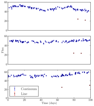
Figure 1: Three simulated data sets, out of a total of 100. It is difficult to infer the lag $\bar{\tau}$ for any of these objects (although there is some information available). See Figure 3 for the $\bar{\tau}$ posterior distributions for these three data sets.

We computed the stacked cross-correlation function for the 100 data sets. The cross-correlation function for a single object is defined as in Fine et al. (2012). For a lag bin between $\tau$ and $\tau+\delta$ the amount of cross correlation is calculated by looping over pairs of points (one selected from the continuum data set, and another from the line data set), and accumulating mass when the lag between the two points is between $\tau$ and $\tau+\delta$.

$$X(\tau;\delta)=$$

$$\frac{\sum_{i=1}^{N_{y}}\sum_{j=1}^{N_{l}}\left(y_{i}-\bar{y}\right)\left(l_{j}-\bar{l}\right)\mathds{1}\left((t_{l_{j}}-t_{y_{i}})\in[\tau,\tau+\delta]\right)}{\sum_{i=1}^{N_{y}}\sum_{j=1}^{N_{l}}\mathds{1}\left((t_{l_{j}}-t_{y_{i}})\in[\tau,\tau+\delta]\right)}$$ (20)

The denominator is the number of pairs of points that fall within the lag range being considered, $[\tau,\tau+\delta]$, denoted $n_{\rm pair}$ by Fine et al. (2012). The stacked cross-correlation function for $N$ objects is sum of the CCFs of the individual objects. In Figure 2, we show the stacked CCF (on a log scale) from our 100 simulated AGN data sets. There is a clear peak around 10 days, and the full width at half maximum, while not strictly well defined, is roughly 0.25 dex.

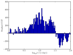
Figure 2: The stacked cross-correlation function of the simulated data. A clear peak is seen around $\tau\approx 10$ days, but the stacked CCF has a large width. It is difficult to interpret the cause of this width, and to determine whether the width is due to uncertainty or diversity in the sample of AGN. These difficulties motivate the hierarchical Bayesian model.

As the data does not contain measurements at all possible time lags, the stacked CCF will always require some smoothing. Here, the smoothing is supplied by the choice of a bin width $\delta$. The stacked CCF has a substantial width. One weakness of the stacked CCF method is that it is not clear whether this width is caused by real diversity in the sample of AGN, or whether it is simply caused by the difficulty in measuring the lag $\bar{\tau}$ of an object with such sparse data. By contrast, the hierarchical Bayesian approach clearly separates these two concepts.

To implement the hierarchical Bayesian approach on the simulated data, we first used the single-object model on each object. The results for three objects (the same three objects shown in Figure 1) are plotted in Figure 3. Due to the sparse data, there is a large amount of uncertainty about the value of $\bar{\tau}$ for each system. Some objects do not allow any real measurement of $\bar{\tau}$, but some do, as a result of fortuitous variability of the continuum.

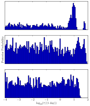
Figure 3: Samples from the posterior distribution for $\log_{10}(\bar{\tau})$ for three objects whose data sets are shown in Figure 1. These posteriors were obtained by analysing each object separately with the single-object model. For the first object, there is a moderate “detection” of a lag at about 10 days (although there is a small second mode above 100 days, which can be understood by inspecting the data in Figure 1). The second object’s lag was not well constrained, and the third object’s data only provided an upper limit on its lag.

Finally, we combined the results from the single-object model into an inference about hyperparameters $\mu$ and $\sigma$ describing the central value and the diversity of $\bar{\tau}$ respectively, using the result of Equation 1. This requires us to know the prior $\pi(\bar{\tau})$ implied by the simple-object model, since we did not assign the prior directly to $\bar{\tau}$ but indirectly through $a$ and $b$. The prior for $\bar{\tau}$ in the single-object model is very well approximated by a log-uniform distribution.

Since lags $\bar{\tau}$ are positive, our assumption for the prior on $\bar{\tau}$ given the hyperparameters is a lognormal distribution with median $\mu$ and width (standard deviation of $\log_{10}(\bar{\tau})$) $\sigma$:

$$\log_{10}(\bar{\tau})\sim\mathcal{N}(\log_{10}(\mu),\sigma^{2})$$ (21)

The joint posterior distribution for $\mu$ and $\sigma$, given the data from $N=100$ AGN, is shown in Figure 4. The prior for $\mu$ and $\sigma$ was uniform inside the rectangle shown, and the posterior distribution covers a much smaller area, indicating that the data contained a lot of information about the hyperparameters. The true values used to generate the simulated data are denoted by the star symbol in Figure 4, and is typical of the posterior distribution, as it should be.

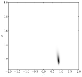
Figure 4: The joint posterior distribution for $\mu$ and $\sigma$, hyperparameters describing the distribution of $\bar{\tau}$ values in the sample. The prior distribution was uniform over the area shown. The true solution $(\mu=0.867,\sigma=0.157)$ is indicated by the white star symbol. $\mu=0.867$ corresponds to a typical lag of 7.4 days.

The marginal posterior distribution for $\mu$ is shown in Figure 5 along with the posterior predictive distribution for the “next” $\bar{\tau}$ value. The inference about $\mu$ can be summarised as $\mu=0.838\pm 0.047$ (consistent with the known input value of $0.867\approx\log_{10}(7.4)$), and the prediction about $\log_{10}(\bar{\tau})$ may be summarised as $\log_{10}(\bar{\tau})=0.838\pm 0.215$. The Bayesian approach has clearly separated the uncertainty about $\mu$ from the diversity of the sample, described by $\sigma$.

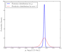
Figure 5: The marginal posterior distribution for $\mu$, the hyperparameter describing the center of the distribution for $\log_{10}\left(\bar{\tau}\right)$, is plotted as the solid line.

Note that our method for combining individual object results into an inference about the population (Section 2) assumes that the hierarchical prior applies to only a single parameter (in our case $\bar{\tau}$). If we incorporate additional information by using a hierarchical prior for the other model parameters, allowing us to detect (for example) that all of the response amplitudes $A$ were equal to 0.5, we may be able to make more accurate inferences. However, this would increase the complexity of the method and the computational expense.

5 Conclusions

Reverberation mapping campaigns are observationally intensive, yet potentially very informative. This has led to research into RM data analysis techniques, as well as less costly observing strategies. The recent approach of Fine et al. (2012) demonstrated that it is possible to combine information from many sparsely-measured AGN and infer properties of the sample rather than insisting on accurate results about a particular object.

In this letter we extended the approach of Fine et al. (2012) by implementing a Bayesian hierarchical model for the data analysis. The main advantage of this approach is a clear interpretation of the output, which is a posterior distribution for hyperparameters describing the sample of AGN.

We demonstrated this approach on a simulated data set consisting of 100 AGN with well-measured continuum light curves but sparsely measured (two epochs per AGN) broad line light curves. For the simulated data set we were able to obtain an inference on $\mu$, a hyperparameter describing the typical value of the lag, to within 0.047 dex (1-$\sigma$ uncertainty), whereas the stacked cross-correlation function had a FWHM of $\sim$ 0.25 dex. This is possible because a subset of the objects in the sample will have a measureable lag. We hope this approach will facilitate informative studies of samples of AGN.

References

- Barth et al. (2013) Barth A. J., et al., 2013, ApJ, 769, 128
- Bentz et al. (2010) Bentz M. C., et al., 2010, ApJ, 720, L46
- Brewer et al. (2011) Brewer B. J., et al., 2011, ApJ, 733, L33
- Brewer, Pártay, & Csányi (2011) Brewer B. J., Pártay L. B., Csányi G., 2011, Statistics and Computing, 21, 4, 649-656. arXiv:0912.2380
- Brewer, Foreman-Mackey, & Hogg (2013) Brewer B. J., Foreman-Mackey D., Hogg D. W., 2013, AJ, 146, 7
- Brewer et al. (2013) Brewer B. J., Marshall P. J., Auger M. W., Treu T., Dutton A. A., Barnabè M., 2013, arXiv, arXiv:1310.5177
- Fine et al. (2013) Fine S., et al., 2013, MNRAS, 434, L16
- Fine et al. (2012) Fine S., et al., 2012, MNRAS, 427, 2701
- Hogg, Myers, & Bovy (2010) Hogg D. W., Myers A. D., Bovy J., 2010, ApJ, 725, 2166
- Kelly (2007) Kelly B. C., 2007, ApJ, 665, 1489
- Kelly, Bechtold, & Siemiginowska (2009) Kelly B. C., Bechtold J., Siemiginowska A., 2009, ApJ, 698, 895
- Krolik & Done (1995) Krolik J. H., Done C., 1995, ApJ, 440, 166
- Li et al. (2013) Li Y.-R., Wang J.-M., Ho L. C., Du P., Bai J.-M., 2013, arXiv, arXiv:1310.3907
- Loredo (2004) Loredo T. J., 2004, AIP Conference Series, 735, 195
- Loredo (2012) Loredo T. J., 2012, arXiv, arXiv:1208.3036
- Hoffman & Gelman (2011) Hoffman M. D., Gelman A., 2011, arXiv, arXiv:1111.4246
- Pancoast, Brewer, & Treu (2011) Pancoast A., Brewer B. J., Treu T., 2011, ApJ, 730, 139
- Pancoast et al. (2012) Pancoast A., et al., 2012, ApJ, 754, 49
- Peterson (2008) Peterson B. M., 2008, NewAR, 52, 240
- Shu et al. (2012) Shu Y., Bolton A. S., Schlegel D. J., Dawson K. S., Wake D. A., Brownstein J. R., Brinkmann J., Weaver B. A., 2012, AJ, 143, 90
- Zu et al. (2013) Zu Y., Kochanek C. S., Kozłowski S., Udalski A., 2013, ApJ, 765, 106
- Zu, Kochanek, & Peterson (2011) Zu Y., Kochanek C. S., Peterson B. M., 2011, ApJ, 735, 80