An investigation into the Gustafsson limit for small planar antennas using optimisation

Abstract

The fundamental limit for small antennas provides a guide to the effectiveness of designs. Gustafsson et al, Yaghjian et al, and Mohammadpour-Aghdam et al independently deduced a variation of the Chu-Harrington limit for planar antennas in different forms. Using a multi-parameter optimisation technique based on the ant colony algorithm, planar, meander dipole antenna designs were selected on the basis of lowest resonant frequency and maximum radiation efficiency. The optimal antenna designs across the spectrum from 570 to 1750 MHz occupying an area of $56mm\times 25mm$ were compared with these limits calculated using the polarizability tensor. The results were compared with Sievenpiper’s comparison of published planar antenna properties. The optimised antennas have greater than 90% polarizability compared to the containing conductive box in the range $0.3<ka<1.1$, so verifying the optimisation algorithm. The generalized absorption efficiency of the small meander line antennas is less than 50%, and results are the same for both PEC and copper designs.

I Introduction

Small antenna theory was introduced by Wheeler [1] for the first time and Chu [2] developed a field based method to find general formulas for the maximum gain $G$, the minimum quality factor $Q$ and the maximum $G/Q$ ratio. Since then Harrington [3], Collin and Rothschild [4], and McLean [5] and many other authors tried to verify and re-examine Chu’s findings. A holistic review on these works is available in [6, 7].

Gustafsson et al [8, 9] proposed a new hypothesis which puts another lower bound on antennas of arbitrary shape. The new bound states the $D/Q$ ratio (or gain-bandwidth product) is directly related to the generalized absorption efficiency and polarizability of the antenna obstacle. The overall antenna performance is directly dependent on the electrostatic polarizability of the antenna. The new limit is close to the actual $Q$ values of antennas while previous bounds sit far lower for real world antennas.

Vandenbosch [10] proposed a new method to calculate $Q$ from the current distribution of the source. He later extended this method to a simple procedure to find the $Q$ of small antennas by making the determinant of a matrix equation zero [11]. Also, an explicit relation has been proved between the actual volume of the antenna and its associated $Q$ factor [12].

Yaghjian and Stuart [13] used a quasi-static approximation to find the $Q$ factor. Their $Q$ has an inverse relationship to the polarizability of the antenna (similar to [8]). In [14], the works of [13] were simplified to find $Q$ for planar structures. In [15, 16], the characteristic modes were employed to compute the $Q$ factor.

Sievenpiper et al [17] recently studied a large number of antenna designs published in IEEE Transactions on Antennas and Propagation, and found that the McLean-Chu limit is a valid bound on the antenna $Q$. Due to the significant role of bandwidth and efficiency in engineering problems, they proposed using the $B\eta_{r}$ limit instead of $Q$. For instance, Kanesan and Thiel [18] concluded that a 28.5% bandwidth was required for planar RFID antennas when placed on objects with electrical properties in the conductivity range $10^{-7}<\sigma<3\times 10^{-2}S/m$ and relative permittivity $1<\epsilon_{r}<6$. Furthermore, the bandwidth plays a key role in the system design of a front end module in which antenna is a part of the whole system.

The Q limit by Chu-McLean is simple and has been used for decades, however, it is usually far from practical for small antenna designs when $ka$ approaches zero. If the radiation efficiency $\eta_{r}$ is less than 100%, then the $Q$ of the antenna decreases proportionally, and $Q/\eta_{r}$ eliminates the dependency of $Q$ to losses in the antenna structure. The Gustafsson method is based on calculating the polarizability tensor. This inherently assumes that the conducting elements are perfectly conducting. This means that the efficiency calculations by Gustafsson will be the highest possible values, but the antenna $Q$ for the lossless cases are close to small antenna designs.

Thiel and Lewis et al [19, 20, 21] employed the Ant Colony Optimization to search for the best performing antennas for a given size in terms of radiation efficiency and lower resonant frequency. Based on a planar meander-line antenna and a square grid pattern, a range of optimised structures were obtained [19, 22] and a review on the effect of radius of the wire segment was reported in [23, 24].

In this paper, we used a set of previously optimized antennas to examine validity of the recent bounds on antennas. The left hand side of the bound in [8] is the directivity and Q-factor which were calculated using the MoM EM simulation package FEKO [25]. To find generalized absorption efficiency $\check{\eta}_{a}$, each antenna was simulated by FEKO over the frequency range of 0.1-50GHz while the resonant frequency is between 0.5-1.7GHz. The polarizability was calculated by our own Method of Moments code for each antenna. In addition to the lossless antennas, the identical antennas with loss are reported in this paper. The main results of the paper are: (1) the polarizability of the meander line is less than the polarizability of the containing box (2) $\check{\eta}_{a}$ is less than 50% for small meander lines, but approaches 50% for the optimised antennas, (3) the values of $\check{\eta}_{a}$ for PEC and copper antennas are almost identical, (4) the different limits on the performance of the lossy antennas are explored, (5) meander line antennas optimised for efficiency and frequency approach the theoretical limit in [8], (6) the $B\eta_{r}$ limit is valid for the complete set of antennas in both lossless and lossy cases.

II Background Theory

The minimum quality factor $Q$ of an small omnidirectional antenna was first derived by Chu [2] and later by Collin [4] and Mclean [5] for linear and circular polarizated TE and TM waves, respectively:

$$Q=\dfrac{1}{ka}+\dfrac{1}{(ka)^{3}}$$ (1)

$$Q=\dfrac{1}{ka}+\dfrac{1}{2(ka)^{3}}$$ (2)

where $k$ and $a$ are the wavenumber and minimum radius of the circumscribing sphere of antenna. Further research by Pozar [26] demonstrated that the lower $Q$ in (2) is the result of simultaneous use of TE and TM modes and not the polarization of the radiated wave.

Sievenpiper et al [17] suggested that instead of calculating $Q$, the Bandwidth-Efficiency product, the following form should be used as a criteria of antenna performance:

$$B\eta_{r}=\dfrac{1}{\sqrt{2}}\left(\dfrac{1}{ka}+\dfrac{1}{n(ka)^{3}}\right)^{-1}$$ (3)

where $\eta_{r}$ is the radiation efficiency in (10) and $B$ is the fractional bandwidth. $n$ is determined by the type of the propagation from the antenna [26, 17]. Equation 3 is called as the first and second order limits when $n$ is selected as 1 and 2 respectively.

Gustafsson et al [8] considered the antenna in the receiving mode and looked to the scattering properties of the antenna. By invoking an optical theorem, if $\hat{e}$ and $\hat{k}$ are the polarization and direction of the wave propagation, one can obtain:

$$\int\limits_{0}^{\infty}\dfrac{\left(1-\arrowvert\Gamma(k)\arrowvert^{2}\right)D}{k^{4}}dk={}\\ {}\dfrac{\check{\eta}_{a}k_{0}^{3}}{2\pi}\Bigg{(}\hat{e}\cdot\gamma_{e}\cdot\hat{e}+\left(\hat{k}\times\hat{e}\right)\cdot\gamma_{m}\cdot\left(\hat{k}\times\hat{e}\right)\Bigg{)}$$ (4)

In (4), $\Gamma$ and $D$ are the antenna reflection coefficient and directivity respectively while $\gamma_{e}$ and $\gamma_{m}$ are the electric and magnetic polarizability of the antenna obstacle. The generalized absorption efficiency, is defined by the ratio of integrated absorption cross section to the sum of the integrated absorption and scattered cross sections:

$$\check{\eta}_{a}=\dfrac{\int\limits_{0}^{\infty}\dfrac{\sigma_{a}}{k^{2}}dk}{\int\limits_{0}^{\infty}\dfrac{\sigma_{a}+\sigma_{s}}{k^{2}}dk}$$ (5)

This can be interpreted as the ratio of the total absorbed power to the sum of total absorbed and scattered powers. Finally, the bound on $D/Q$ ratio can be written as:

$$\dfrac{D}{Q}\leq{}\dfrac{\check{\eta}_{a}k_{0}^{3}}{2\pi}\Bigg{(}\hat{e}\cdot\gamma_{e}\cdot\hat{e}+\left(\hat{k}\times\hat{e}\right)\cdot\gamma_{m}\cdot\left(\hat{k}\times\hat{e}\right)\Bigg{)}$$ (6)

It is important to note that as long as no magnetic material is present in the structure $\gamma_{m}$ should be assumed zero [8].

Yaghjian and Stuart [13] used a quasi-static approximation to write a bound on $Q$ in terms of antenna volume $V$ and polarizability $\gamma$.

$$Q_{Y,lb}=\frac{6\pi}{k^{3}\gamma}(1-V/\gamma)$$ (7)

The limit in [13] can be applied for both planar and non-planar antennas.

As suggested by Mohammadpour Aghdam et al  [14], planar structures cannot approach the bounds for spherical shapes (i.e. Chu limit). They considered the fact that one can neglect the volume of the planar antennas, and simplified (7) in the following form:

$$Q_{rect,lb}=\dfrac{9/2}{(ka)^{3}}\dfrac{1}{\gamma_{l}^{n}}$$ (8)

where $\gamma_{l}^{n}$ is ratio of the polarizability of the meander line normalized to the polarizability of the enclosing rectangle. The Q from (8) is the lowest possible value for a non-magnetic planar structure. However, the bounds from [8] and [13] can include the effect of the magnetic materials.

III Method

The Ant Colony algorithm by Lewis et al [20, 21] used a rectangular matrix of points through which the conducting meander line passed (see Fig. 1). The line was terminated when the end of the line has no further option but to join an existing line. The overall size of the planar antenna was $56mm\times 25mm$ which gives an aspect ratio of 2.24. This is close to the maximum performance identified by Gustafsson et al (maximum 1.96). The antenna optimisation was conducted using NEC as the solver [27]. These meander line antennas are studied in [28], in terms of their $Q$ factor and figure of merit (FOM). After optimization, FEKO was used to do all of the EM calculations regarding $Q$ factor, radiation and generalized absorption efficiencies, etc using segment mesh elements. The electrostatic computation of polarizability, was done using our own code which solves the problem using triangular mesh elements.

Also, to make a comparison with state of the art antennas, a RFID tag antenna, and a H-shape antenna were included in this investigation.

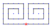
(a) 576MHz

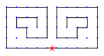
(b) 596MHz

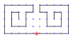
(c) 660MHz

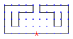
(d) 724MHz

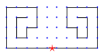
(e) 790MHz

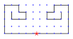
(f) 912MHz

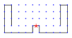
(g) 1120MHz

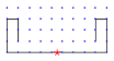
(h) 1320MHz

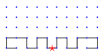
(i) 1757MHz

(j) 1071MHz

(k) 1116MHz

Figure 1: Geometry of antenna and grid points (red $\star$ shows position of the feed). (a)-(i) are optimized antennas (j) RFID tag (k) H-Shape antenna [29].

In order to compute Gustafsson’s limit, the previously optimized antennas were analysed using the procedure in [30]; first the optimized lossy antennas were analysed in transmission mode to derive the impedance and gain using FEKO [25]. Figure 2 shows the reflection coefficient of all antennas. We therefore calculated the Q factor using the Yaghijian-Best formula [31] which is valid under the assumption that the impedance at the resonance is well approximated by a single mode resonance:

$$Q=\dfrac{\omega}{2R_{0}(\omega)}\sqrt{[R^{\prime}(\omega)]^{2}+[X^{\prime}(\omega)+{X(\omega)/\omega}]^{2}},$$ (9)

where $\omega$ is resonant radian frequency, $R_{0}(\omega)$, and $X_{0}(\omega)$ are the resistance and reactance of antenna, while $R_{0}^{\prime}(\omega)$, and $X_{0}^{\prime}(\omega)$ are the slope of the $R_{0}(\omega)$, and $X_{0}(\omega)$. This formulation assumes a single resonance.

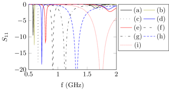
Figure 2: S-parameters of the antennas in Fig. 1.

The radiation efficiency was computed using the method in [32] which works with the summation of the loss terms in each segment of lossy wire antenna. When $R_{in}$ is the input impedance, $I$ is the current at the feed, $r$ is the radius of the wire, $f$ is the frequency, $\mu_{0}$ is the permittivity of free space, $\sigma$ is the conductivity of the conductor, $l$ is the length of the wire segment, $i_{i}$ is the current in the segment $i^{th}$, $\eta_{r}$ can be found from:

$$\eta_{r}=\dfrac{R_{in}I^{2}-\sqrt{\dfrac{\pi f\mu_{0}}{\sigma}}\dfrac{l}{2\pi r}\sum\limits_{i=1}^{N}i_{i}^{2}}{R_{in}I^{2}}.$$ (10)

The antenna was centrally loaded by the impedance of the antenna at the first resonance. A co-polarized plane wave in the boresight of the antenna was used as the excitation in FEKO to find absorbed and scattered cross sections by the antenna.

The polarizability calculation can be started from the following integral form of Laplace’s equation

$$x_{j}+C_{j}=\iint\limits_{\partial S}\frac{\rho_{j}({x}^{\prime})}{4\pi\left|x-{x}^{\prime}\right|}d{S^{\prime}},$$ (11)

where $\rho_{j}$ is the surface charge density when the object is located in a static field of the unit amplitude in the $\hat{x}_{j}$ direction and integration is over the surface of the geometry $\partial S$. $x$ and $x^{\prime}$ refer to observation and source points, respectively. $C_{j}$ is selected in such a way that the total charge on the object is zero:

$$\iint\limits_{\partial S}\rho_{j}dS^{\prime}=0.$$ (12)

We used MoM with pulse basis functions to solve (11). After finding $\rho_{j}$ over $\partial S$, the polarizability in the $\hat{x}_{i}$ direction due to applied field in $\hat{x}_{j}$ is:

$$\gamma_{ij}=\iint\limits_{\partial S}x_{i}\rho_{j}\left(x\right)dS.$$ (13)

With this method [33], polarizability of each optimized antenna was computed. The method was verified using direct comparison with theoretical values for spheroids [33]. Fig. 3 demonstrates that the code shows very good convergence with an increasing number of mesh elements. The existance of corners in the meander antennas results in less accuracy and slower congegence.

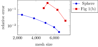
Figure 3: Convergence comparison of polarizability calculations for a sphere (circle) and meander antenna design in Fig. 1(b) (square).

Matlab was used to compute theoretical parameters from the results of the radiation and scattering simulations. For both transmitting and receiving mode, the conductivity of the wires was assumed to be that of copper $(5.7\times 10^{7}S/m)$.

It is rather straight forward to calculate the other bounds on $Q$ [13, 14] once the polarizability is computed. It should be noted that the polarizability of each antenna should be directly substituted in (7), while (8) needs the polarizability of antenna normalized to polarizability of the equivalent rectangle.

IV Results

IV-A Polarizablity

Figure4 shows the normalized polarizability of nine optimized meander line antennas $\gamma_{ml}$ as a function of the semi-axis ratio $\xi=l_{1}/l_{2}$. The polarizability of the designs are compared with the polarizability of the $(l_{1}+2r)\times(l_{2}+2r)$) infinitely thin rectangle $\gamma_{rv}$, and the polarizability of the ($l_{1}\times l_{2}\times 2r$) parallelepiped boxes $\gamma_{b}$ where $r$ is radius of the wire. For all antennas in this study, $l_{1}$ and $r$ were set to $56mm$, $1mm$, but $l_{2}$ varies from $25mm$ to $6.25mm$. The polarizability of the rectangle is available from [34] in the following forms for $(\xi<1)$ and $(\xi>1)$ cases respectively:

$$\frac{\gamma_{rv}}{a^{3}}\approx\xi^{2}\frac{2\pi-5.215\xi-0.108\xi^{2}}{1-1.162\xi+1.712\xi^{2}-1.222\xi^{3}},$$ (14)

$$\frac{\gamma_{rv}}{\gamma_{sv}}\approx\frac{1.001+18.098\xi^{-1}-11.42\xi^{-2}+2.266\xi^{-3}}{1+17.074\xi^{-1}-0.309\xi^{-2}+24.78\xi^{-3}},$$ (15)

In (15), $\gamma_{sv}$ is the polarizability of the spheroid which is available from [34]. We also emphasise that polarizability of the box should be used in the calculation of the lower bound [14] on the $Q$.

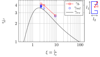
Figure 4: Polarizability versus length to width ratio ( box containing antenna, meander line antenna, rectangle)

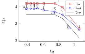
Figure 5: $\gamma_{ml}$: normalized polarizability of the meander line, $\gamma_{b}$: normalized polarizability of a conducting box of dimension $l_{1}\times l_{2}\times 2r$, $\gamma_{rv}$: normalized polarizability of the infinitely thin rectangle $l_{1}\times l_{2}$. The letter references are from Fig. 1.

It is seen that the polarizability of the meander lines are less than the polarizability of the parallelepiped box which is expected from the bounds on the polarizability of the objects in [35]. The reason the meander line result is higher than the rectangle result is due to the finite thickness of the wires compared to the infinitely thin rectangle.

Variation of the polarizability of the designs with the electrical length is shown in Fig.5. It is interesting to note that the lower polarizabilities are obtained for the antennas with higher $ka$ values. In Fig.4, 5, the polarizabilities are normalized with respect to $a^{3}$ where $a$ is the radius of the circumscribing sphere of the antenna. For small $ka$ optimised meander lines have approximately 90% polarizability of the box. For $ka\geq 1$ optimised antennas have almost 99.1% polarizability of the containing box.

IV-B Radiation Efficiency

Figure 6 shows the radiation efficiency $\eta_{r}$ of the meander line antennas computed from (10). As expected, the radiation efficiency approaches 100% as the resonant frequency increases. This is expected as antennas with larger electrical length have a larger radiation resistance which leads to a higher $\eta_{r}$.

IV-C Generalized Absorption Efficiency

One of the parameters to be calculated is the generalized absorption efficiency $\check{\eta}_{a}$ (see (5)) which can be computed by two methods: the first method comes from the direct calculation of the absorption and extinction cross sections $\sigma_{a}$ and $\sigma_{ext}$ . Therefore, simulating the antenna loaded with the resonant impedance in the receiving mode is of interest while a plane wave illuminates the antenna. Absorbed and scattered cross sections have a direct relation with absorbed and scattered power [36]:

$$\sigma_{a}=\dfrac{1}{240\pi}\dfrac{P_{r}}{\arrowvert E_{i}\arrowvert^{2}}$$ (16)

$$\sigma_{ext}=\dfrac{1}{240\pi\arrowvert E_{i}\arrowvert^{2}}\times\\ \Bigg{[}P_{r}+P_{loss}+\int\limits_{0}^{\pi}\int\limits_{0}^{2\pi}\arrowvert E_{s}(\theta,\phi)\arrowvert^{2}\sin(\theta)d\theta d\phi\Bigg{]}$$ (17)

where $P_{r}$, $P_{loss}$, $E_{i}$ and $E_{s}$ are the absorbed power in the load, dissipated power in the lossy material, incident and scattered electric field strength, respectively. It should be noted that $P_{loss}$ has to be considered for the lossy antennas. The second method is to simulate the antenna in the transmitting mode and find directivity $D$ and reflection coefficient $\Gamma$. The absorption cross section was found for lossless antennas from [8, 30]:

$$\sigma_{a}=\dfrac{\pi D(k)}{k^{2}}\bigg{[}1-\arrowvert\Gamma(k)\arrowvert^{2}\bigg{]}$$ (18)

On the other hand, the forward scattering sum rule is useful to find the overall extinct power by the antenna obstacle [8, 30].

$$\int\limits_{0}^{\infty}\dfrac{\sigma_{ext}}{k^{2}}dk=\dfrac{\pi}{2}\gamma_{\infty}$$ (19)

Equation (19) can be directly used to find $\check{\eta}_{a}$, however, numerical integration of equations (16-19) should be performed over broad range of frequencies to yield the $\check{\eta}_{a}$. Both of these methods were used in calculations to ensure accuracy of the simulations.

Variations in $\check{\eta}_{a}$ with $ka$ is illustrated in the Fig. 7 for both lossy and lossless antennas. It shows that for a small antenna $\check{\eta}_{a}$ is less than 50% and approaches 50% for antennas with larger $ka$. Therefore, especially for electrically small antennas, one should not estimate the generalized absorption efficiency as 50%. However, one should compute $\check{\eta}_{a}$ with the highest possible accuracy due to its crucial role in equation (6).

Another important result in Fig. 7 is that $\check{\eta}_{a}$ is not sensitive to the conductivity of the material. Figure. 7 shows that the change from PEC to copper makes a little difference to the $\check{\eta}_{a}$ values.

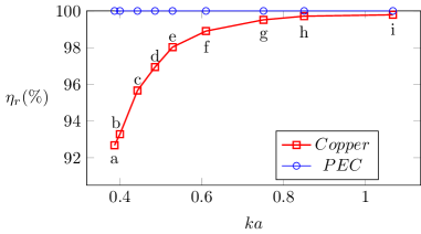
Figure 6: Comparison of the radiation efficiency of the copper and PEC antennas

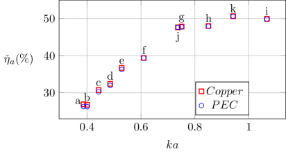
Figure 7: Explicit values $\check{\eta}_{a}$ for the lossy and lossless antennas while each antenna is loaded with a matched impedance at the resonant frequency.

A comparison between the absorbed and scattered cross sections ($\sigma_{a}$ and $\sigma_{s}$) of the optimized meander line antennas with a classic dipole antenna provides some intuitive explanation. The dipole antenna is tuned to resonate at 596MHz with 244.2mm length and length to diameter ratio of 1000. Absorbed and scattered cross sections are normalized and depicted in the Fig.8 on logarithmic plot. Similar to the results in [8], $\sigma_{a}$ and $\sigma_{s}$ of the dipole follow each other in the first resonance, and they have a descending magnitude envelope and bandwidth in the higher resonances. In the case of meander line antennas, the sharpest resonance is the first resonance, and $\sigma_{s}$ is much greater than the $\sigma_{a}$ over a broad range of frequencies. This means that the overall integration of the $\sigma_{a}$ and $\sigma_{a}+\sigma_{s}$ leads to $\check{\eta}_{a}\leq$50%.

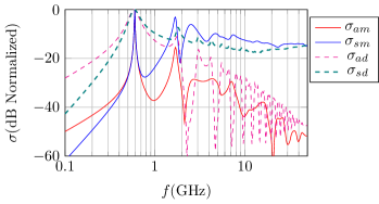
Figure 8: logarithmic plot of $\sigma_{am}$, $\sigma_{sm}$ absorption and scattering cross section of meander line (Fig.1(b)), $\sigma_{ad}$, $\sigma_{sd}$ absorption and scattering cross section of dipole

IV-D $Q$ factor

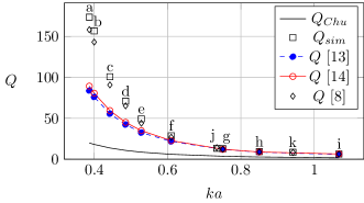
Figure 9: Comparison of the bounds on $Q$ by Chu, Yaghjian [31], Mohammadpour[14], Gustafsson [8] with the practical $Q$ values.

The $Q$ factor of the designs was compared with the limits by Chu [2], Gustafsson et al [8], Yaghjian et al [13] and Mohammadpour Aghdam et al [14]. As is shown in Fig. 9, the bound by Chu is obviously much lower than the actual $Q$ even for large values of $ka$. Predictions from [13, 14] are close together since antennas in this study do not include magnetic materials. Limits from [13, 14] are closer to the practical designs for the antennas confined in $ka>0.5$. On the other hand, the limit in [8] is capable of accurately predicting $Q$ values even for small values of $ka$. We emphasise that close predictions from Gustafsson limit happen since $\check{\eta}_{a}$ is rigorously calculated for each antenna separately.

The volume of the antennas decreases sequentially from Fig. 1(b) to Fig. 1(i). A general design tip proved in [12] states any increase in the actual volume, in any direction, yields a smaller $Q$ when the antenna boundaries are fixed. It should be emphasised that a decrease in $Q$ from a decrease in the antenna volume in this paper is not contrary to [12]. The implied assumption in [12] is that the frequency is unchanged. However, the antennas in the Fig. 1 have different resonant frequencies.

IV-E Bandwidth-Radiation Efficiency Product

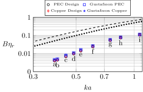
Figure 10: First and second order $B\eta_{r}$ limit, calculated $B\eta_{r}$ for copper and PEC planar antennas, and $B\eta_{r}$ from Gustaffson’s bound.

Figure.10 shows the $B\eta_{r}$ plotted as a function of $ka$ for 9 selected optimized antennas. Criterion for bandwidth $B$ is the range $VSWR\leq 2$ similar to the work in [17]. Included in this graph are the first and second order limits (3) from Sievenpiper et al [17]. The theoretical limits from Gustafsson et al [8] are also shown. The results for the optimised antennas show a continuous trend similar to that for the limits from Sievenpiper et al for spherical antennas. The calculation method from Gustafsson for this antennas lies slightly above the results calculated using the method explained in previous sections.

V Conclusions and further work

Fundamental limits for a set of optimized meander line antennas were analysed in this paper and compared with state of the art antennas from literature. Generalized absorption efficiency $\check{\eta}_{a}$ and polarizability of the antenna were computed for each of the antennas. The paper shows that the polarizability of the meander line antennas are bounded by the polarizability of the equivalent box. The computed generalized absorption efficiency illustrates that (a) $\check{\eta}_{a}<$50% for small meander lines, but approaches 50%, (b) $\check{\eta}_{a}$ is the same for PEC and Copper antennas. Furthermore, recent limits can be reduced to the same expression for a small electric dipole antennas [8, 9, 13, 14]. Finally, $B\eta_{r}$ product were studied and validated for the whole set of antennas in both lossless and lossy cases. This paper has examined mathematical tools which allow antenna designers to compare their results with the theoretical absolute limits. The design challenge remains to find new small antenna structures which better approach the fundamental limits.

References

- [1] H. Wheeler, “Fundamental limitations of small antennas,” Proc. IRE, vol. 35, no. 12, pp. 1479 – 1484, Dec. 1947.
- [2] L. J. Chu, “Physical limitations of omni-directional antennas,” J. Appl. Phys., vol. 19, no. 12, pp. 1163–1175, 1948.
- [3] R. Harrington, “On the gain and beamwidth of directional antennas,” IRE Transactions on Antennas and Propagation, vol. 6, no. 3, pp. 219 –225, Jul 1958.
- [4] R. Collin and S. Rothschild, “Evaluation of antenna Q,” IEEE Trans. Antennas Propag., vol. 12, no. 1, pp. 23 – 27, Jan 1964.
- [5] J. S. McLean, “A re-examination of the fundamental limits on the radiation Q of electrically small antennas,” IEEE Trans. Antennas Propag., vol. 44, no. 5, p. 672, May 1996.
- [6] R. C. Hansen and R. E. Collin, Small Antenna Handbook. John Wiley & sons-IEEE press, 2011.
- [7] J. L. Volakis, C. C. Chen, and K. Fujimoto, Small Antennas Miniaturization Techniques and Applications. McGraw-Hill, 2010.
- [8] M. Gustafsson, C. Sohl, and G. Kristensson, “Illustrations of new physical bounds on linearly polarized antennas,” IEEE Trans. Antennas Propag., vol. 57, no. 5, pp. 1319 –1327, May 2009.
- [9] ——, “Physical limitations on antennas of arbitrary shape,” Proc. R. Soc. A, vol. 463, no. 2086, pp. 2589–2607, 2007.
- [10] G. Vandenbosch, “Reactive energies, impedance, and factor of radiating structures,” IEEE Trans. Antennas Propag., vol. 58, no. 4, pp. 1112 –1127, April 2010.
- [11] ——, “Simple procedure to derive lower bounds for radiation of electrically small devices of arbitrary topology,” IEEE Trans. Antennas Propag., vol. 59, no. 6, pp. 2217 –2225, June 2011.
- [12] ——, “Explicit relation between volume and lower bound for Q for small dipole topologies,” IEEE Trans. Antennas Propag., vol. 60, no. 2, pp. 1147 –1152, Feb. 2012.
- [13] A. Yaghjian and H. Stuart, “Lower bounds on the Q of electrically small dipole antennas,” IEEE Trans. Antennas Propag., vol. 58, no. 10, pp. 3114 –3121, Oct. 2010.
- [14] K. Mohammadpour-Aghdam, R. Faraji-Dana, G. Vandenbosch, S. Radiom, and G. Gielen, “Physical bound on Q factor for planar antennas,” in Eur. Microw. Conf., Oct. 2011.
- [15] J. Chalas, K. Sertel, and J. Volakis, “Q limits for arbitrary shape antennas using characteristic modes,” in IEEE EuCAP,, march 2012.
- [16] M. Capek, P. Hazdra, and J. Eichler, “A method for the evaluation of radiation q based on modal approach,” IEEE Trans. Antennas Propag., vol. 60, no. 10, pp. 4556– 4567, Dec. 2012.
- [17] D. Sievenpiper, D. Dawson, M. Jacob, T. Kanar, S. Kim, J. Long, and R. Quarfoth, “Experimental validation of performance limits and design guidelines for small antennas,” IEEE Trans. Antennas Propag., vol. 60, no. 1, pp. 8 –19, Jan. 2012.
- [18] M. Kanesan, D. V. Thiel, and S. G. O’Keefe, “The effect of lossy dielectric objects on a UHF RFID meander line antenna,” in IEEE Antennas Prop. Symp., Jul 2012.
- [19] A. Galehdar, D. V. Thiel, A. Lewis, and M. Randall, “Multiobjective optimization for small meander wire dipole antennas in a fixed area using ant colony system,” Int. J. RF Microw. Comput-Aid. Eng., vol. 19, no. 5, pp. 592–597, 2009.
- [20] A. Lewis, G. Weis, M. Randall, A. Galehdar, and D. Thiel, “Optimising efficiency and gain of small meander line RFID antennas using ant colony system,” in IEEE Congress on Evolutionary Computation, 2009, May 2009.
- [21] A. Lewis, M. Randall, A. Galehdar, D. Thiel, and G. Weis, “Using ant colony optimisation to construct meander-line RFID antennas,” in Biologically-Inspired Optimisation Methods, ser. Studies in Computational Intelligence, A. Lewis, S. Mostaghim, and M. Randall, Eds. Springer Berlin Heidelberg, 2009, vol. 210, pp. 189–217.
- [22] G. Weis, A. Lewis, M. Randall, A. Galehdar, and D. Thiel, “Local search for ant colony system to improve the efficiency of small meander line RFID antennas,” in 2008 IEEE Congress on Evolutionary Computation (CEC 2008), 2008.
- [23] A. Galehdar, D. Thiel, and S. O’Keefe, “Tapered wire antenna design for maximum efficiency and minimal environmental impact,” in Proc. IEEE ISAPE, 2008, pp. 23–26.
- [24] ——, “Tapered meander line antenna for maximum efficiency and minimal environmental impact,” IEEE Antennas Wireless Propag. Lett., vol. 8, pp. 244–247, 2009.
- [25] FEKO 6.1.1, EM Software and Systems, 1998-2011.
- [26] D. Pozar, “New results for minimum Q, maximum gain, and polarization properties of electrically small arbitrary antennas,” in IEEE EuCAP, 2009.
- [27] G. J. Burke and A. J. Poggio, Numerical Electromagnetics Code (NEC), : National Technical Information Service (U.S. Department of Commerce), 1981.
- [28] M. Shahpari, D. V. Thiel, and A. Lewis, “Exploring the fundamental limits of planar antennas using optimization techniques,” in IEEE Antennas Propagat. Soc. Symp. Dig., 2013, pp. 764–765.
- [29] B. L. G. Jonsson and M. Gustafsson, “Limitations on the effective area and bandwidth product for array antennas,” in URSI Int. Symp. Electromagnetic Theory (EMTS), 2010, pp. 711–714.
- [30] M. Gustafsson, M. Cismasu, and S. Nordebo, “Absorption efficiency and physical bounds on antennas,” Int. J. Antennas Propag., vol. 2010, 2010.
- [31] A. Yaghjian and S. Best, “Impedance, bandwidth, and Q of antennas,” IEEE Trans. Antennas Propag., vol. 53, no. 4, pp. 1298–1324, 2005.
- [32] A. Galehdar, D. Thiel, and S. O’Keefe, “Antenna efficiency calculations for electrically small RFID antennas,” IEEE Antennas Wireless Propag. Lett., vol. 6, pp. 156–159, 2007.
- [33] M. Shahpari, D. V. Thiel, and A. Lewis, “Polarizablity of 2d and 3d conducting objects using method of moments,” ANZIAM Journal, vol. 54, pp. C446–C458, 2013. [Online]. Available: http://journal.austms.org.au/ojs/index.php/ANZIAMJ/article/view/6405
- [34] M. Gustafsson, “Physical bounds on antennas of arbitrary shape,” in Loughborough Antennas and Propagation Conference (LAPC), Nov. 2011.
- [35] D. Sjöberg, “Variational principles for the static electric and magnetic polarizabilities of anisotropic media with perfect electric conductor inclusions,” J. Phys. A-Math. Theor., vol. 42, p. 335403, 2009.
- [36] S. Best and B. Kaanta, “A tutorial on the receiving and scattering properties of antennas,” IEEE Antennas Propag. Mag., vol. 51, no. 5, pp. 26 –37, oct. 2009.