What controls the temperature of a soft mode-driven structural phase transition?

Abstract

We have used an effective model of ferroelectric PbTiO₃, which displays a representative soft mode-driven phase transition, to investigate how different features of the potential-energy surface affect the transition temperature $T_{\rm C}$. We find that the energy difference between PbTiO₃’s high-symmetry (cubic) and low-symmetry (tetragonal) phases (which we call ground state energy $E_{gs}$) is the parameter that most directly and strongly determines $T_{\rm C}$. We have also found that other simple features of the energy landscape, such as the amplitude of the distortion connecting the high-symmetry and low-symmetry structures, can be used as a predictor for $T_{\rm C}$ only as long as they are correlated with the magnitude of $E_{gs}$. We discuss how our results relate to the expected behaviors that can be derived from simpler theoretical approaches, as well as to phenomenological studies in the literature. Our findings support the empirical rule for estimating $T_{\rm C}$ proposed by Abrahams et al. [Physical Review 172, 551 (1968)] and clarify its physical interpretation. The evidence also suggests that deviations from the expected behaviors are indicative of complex lattice-dynamical effects involving strong anharmonic interactions (and possibly competition) between the soft phonon driving the transition and other modes of the material.

I Introduction

Structural phase transitions driven by soft phonon modesBlinc and Žekš (1974); Dove (2005) receive much attention for both fundamental and technological reasons. The occurrence of a soft mode is accompanied by a variety of striking effects, such as very large responses (elastic, dielectric, piezoelectric) and highly tunable properties, that can be exploited in applications. Hence, there is interest in controlling the transition temperature $T_{\rm C}$, as this will in turn determine the functional properties of the material at specific (e.g., ambient) conditions. This interest is being refueled by evidence that tuning the structural behavior provides us with convenient strategies to enhance other important properties, such as the magnetoelectric response.Wojdeł and Íñiguez (2010)

From a designer’s perspective, it would be useful to have simple rules to estimate $T_{\rm C}$ from limited information about a compound. In particular, if we were able to identify a simple predictor that allowed us to guess $T_{\rm C}$ from routine first-principles calculations, we could accelerate the discovery of materials that take advantage of soft mode-related effects. Such a knowledge would also be relevant to the construction of effective potentials for simulations of lattice-dynamical phenomena, as it would tell us which key properties the models must reproduce to render accurate $T_{\rm C}$’s.

The simplest atomistic model that captures the essence of a soft mode-driven transition may be the so-called discrete $\phi^{4}$ model.Bruce (1980) The potential energy is written as

$$E=\sum_{i}\left[\frac{A}{2}u_{i}^{2}+\frac{B}{4}u_{i}^{4}\right]+\frac{C}{2}\sum_{ii^{\prime}}^{\rm n.n.}(u_{i}-u_{i^{\prime}})^{2}\,,$$ (1)

which can be viewed as a Taylor series, around a reference structure of zero energy, as a function of local structural distortions $u_{i}$ defined at every cell $i$. The collective condensation of these local modes reduces the energy of the material according to a double-well potential ($A<0$, $B>0$) like the one sketched in Fig. 1(a). Each local mode is coupled to its nearest neighbors (n.n.) by a spring constant $C$ (here we take $C>0$) that determines the dispersion of the associated phonon band [see Fig. 1(b)]. Within this model, $E_{gs}=-A^{2}/4B$ is the energy per cell of the ground state structure, which is characterized by $u_{i}=u_{gs}=\sqrt{-A/B}$ $\forall i$. This low-energy phase is reached from the high-symmetry structure ($\langle u_{i}\rangle=0$ $\forall i$, where $\langle...\rangle$ denotes thermal average) when we bring the system below $T_{\rm C}$. Note that $|E_{gs}|$ roughly quantifies the thermal energy that the system needs to jump between equivalent potential wells and thus stabilize the high-symmetry phase. Hence, it is tempting to assume

$$k_{\rm B}T_{\rm C}\sim|E_{gs}|=A^{2}/4B\,,$$ (2)

where $k_{\rm B}$ is Boltzmann’s constant. Since the calculation of $E_{gs}$ from first-principles is a trivial task, this would be a very convenient $T_{\rm C}$ predictor.

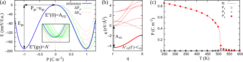
Figure 1: (Color online) Panel (a): The thick solid line represents the double well potential corresponding to the FE instability of our model for PTO. We also show energy wells corresponding to modified potentials, denoted “(Ti–O)⁴” in the text, in which either the ground state polarization ($\Delta P_{gs}\neq 0$) or the ground state energy ($\Delta E_{gs}\neq 0$) has changed. The parameters characterizing the energy surface, and mentioned in the text, are indicated. Note that $A_{\rm FE}=\partial^{2}E/\partial P^{2}$ evaluated at $P=0$, while $A^{\prime}=\partial^{2}E/\partial P^{2}$ evaluated at $P=P_{gs}$. Panel (b): Harmonic force constants of the cubic phase of our PTO model, along the $\Gamma-X$ direction of the first Brillouin zone. We indicate the key parameters mentioned in the text. We use a thicker line to highlight the transversal-optical band corresponding to the FE instability. Note that $C_{\rm FE}=\partial^{2}A_{\rm FE}/\partial q^{2}$, for $q$ along the $\Gamma-X$ line and evaluated at $\Gamma$. Panel (c): Temperature dependence of the polarization as obtained from Monte Carlo simulations of our reference PTO model. The line corresponds to the fit to the model function described in the Appendix.

However, a more careful analysis suggests that the above choice might not be optimal. Within the mean-field approximation,Bruce (1980) it is possible to solve the $\phi^{4}$ model in the displacive ($|A|/C\ll 1$) and order-disorder ($|A|/C\gg 1$) limits (i.e., for strongly- and weakly-coupled local modes, respectively). In both cases we get

$$k_{\rm B}T_{\rm C}\sim Cu_{gs}^{2}=C|A|/B\,.$$ (3)

This predictor gathers information about the magnitude of the structural instability (quantified by $u_{gs}^{2}$ instead of $|E_{gs}|$) and the energy cost for the occurrence of alternative, inhomogeneous distortions (given by $C$).

Finally, it has been found empiricallyAbrahams et al. (1968) that $T_{\rm C}$ correlates with the magnitude of the symmetry-breaking distortion, so that

$$T_{\rm C}\sim u_{gs}^{n}\,,$$ (4)

where $n$ is a positive integer. By examining the structural phase transitions of a variety of ferroelectric compounds, the authors of Ref. Abrahams et al., 1968 concluded that, to fit their data, $n$ can be chosen to be either 1 or 2. Yet, they argue that $n=2$ renders a physically sounder relation, an interpretation that was backed shortly after by the theoretical work of Lines.Lines (1969); Lines and Glass (1977) It has been shown more recentlyGrinberg and Rappe (2004); Juhas et al. (2004) that Eq. (4) with $n=2$ renders a good description for the ordering temperatures of a family of ferroelectric relaxor perovskites.

The above mentioned laws have intriguing implications. For example, the validity of Eq. (4) suggests that either the mean-field result of Eq. (3) is not realistic or that the parameter $C$ adopts similar values in all the materials that were investigated in Refs. Abrahams et al., 1968; Grinberg and Rappe, 2004; Juhas et al., 2004. Also, the validity of Eqs. (2) or (4) might imply that $T_{\rm C}$ does not significantly depend on the energetics of distortions not present in the ground state. Further, Eqs. (3) and (4) suggest that one may encounter materials with very strong instabilities, even with $|E_{gs}|\gg Cu_{gs}^{2}$, that might nevertheless display a relatively low $T_{\rm C}$ determined by relatively small values of $u_{gs}$ and $C$. These are all rather surprising notions.

To shed light on these issues, we conducted a series of numerical experiments using a model potential for PbTiO₃ (PTO). PTO presents a prototypic structural transition, between high-temperature cubic and low-temperature tetragonal structures, and is representative of the class of materials for which empirical rules like Eq. (4) have been observed to hold. The employed model describes PTO in full atomistic detail, and its parameters can be modified by hand to study the resulting changes in $T_{\rm C}$. We can thus test the performance of the predictors mentioned above.

II Computational experiments

Our model for PTO is described in Ref. Wojdeł et al., 2013, where it is labeled “$L^{I}$”. It can be viewed as a Taylor series of the energy, around the ideal cubic perovskite structure, as a function of all possible atomic distortions and strains. The series was truncated at 4th order and only pairwise interaction terms were included. Hence, in essence, our PTO model can be seen as an extended version of the $\phi^{4}$ Hamiltonian in which all the degrees of freedom are treated explicitly. The potential parameters were computed by using the local density approximation (LDA) to density functional theory. To compensate for LDA’s well-known overbinding problem, we simulate the model under the action of a tensile hydrostatic pressure of 14.9 GPa.

The potential well associated with the ferroelectric (FE) instability of our model for PTO is shown in Fig. 1(a). When we solve the model by running Monte Carlo (MC) simulations in a periodically repeated box of 10$\times$10$\times$10 unit cells, we obtain an abrupt transition at $T_{\rm C}\approx$ 510 K,fnT as reflected in the $T$-dependence of the polarization ($P$) in Fig. 1(c). In order to get reliable results for atomic displacements and strains (from which we derive the spontaneous polarization as described in Ref. Wojdeł et al., 2013), we ran at least 20,000 MC sweeps for thermalization, followed by at least 20,000 additional sweeps to compute thermal averages. For temperatures close to the transition, the simulations were run for up to 80,000 MC sweeps after thermalization in order to obtain well converged values. We initialized all our simulations, for all models and temperatures, from the same cubic reference state; hence, our results do not display any hysteretic behavior. For the original model, we also ran simulations in which, for each new temperature $T+\Delta T$, we used a representative configuration of the previous temperature considered $T$ to initialized the MC simulations; we found that the hysteresis, if present, is narrower than what we claim for the accuracy of the $T_{\rm C}$ determination.fn- From the obtained thermal averages, we estimate $T_{\rm C}$ by a simple and robust fitting to the $P(T)$ profile, as described in the Appendix.

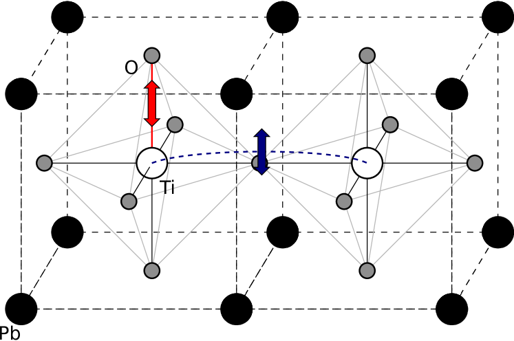
Figure 2: Sketch of the Ti–O and Ti–Ti interactions that we modified in our models. We worked in the displacement-difference representation introduced in Ref. Wojdeł et al., 2013. In the Ti–O case, the interaction involves displacements along the direction defined by the pair of atoms involved; it can be easily seen that they do not affect the energetics of the O₆ octahderal rotations discussed in Section III. In the Ti–Ti case, the interaction involves displacements orthogonal to the direction defined by the pair of atoms involved. The modified interaction controls the transversal modulation of the FE instability as we move away from the center of the Brillouin zone.

We began by checking how the separate variations of the ground state energy $|E_{gs}|$ and polarization $P_{gs}$ affect $T_{\rm C}$. To do so, we constructed models whose associated energy wells are shown in Fig. 1(a). Such models were obtained by tuning some of the interactions controlling the FE instability, namely, the harmonic and 4th-order couplings between neighboring Ti and O atoms (see sketch in Fig. 2). We were thus able to (1) change $E_{gs}$ while keeping $P_{gs}=P_{gs}^{0}$, where the “0” superscript denotes values corresponding to our unmodified PTO model, and (2) shift $P_{gs}$ while keeping $E_{gs}=E_{gs}^{0}$. (We also worked with Pb–O couplings and obtained very similar results for the behavior of $T_{\rm C}$.) All the modified models we studied present the same qualitative behavior, and the atomic distortions characterizing the FE phase resemble closely those occurring in real PTO. Note that large changes in the potential parameters can eventually lead to qualitatively different behaviors (e.g., suppression of ferroelectricity, change of polar axis), which limited our ability to tune the models. Finally, let us mention that the potential parameters we modified do not interfere with the energetics of the PTO modes involving rotations of the oxygen octahedra; hence, our changes did not affect significantly the instability competition discussed below.

Note that we decided to use $P_{gs}$ as a measure of the total distortion $u_{gs}$. Besides its historical motivation,Abrahams et al. (1968) this choice is reasonable because in PTO all the individual atomic displacements, as well as the cell strain, add up to the total polarization of the ground state. (See caption of Table I for some detail on how these quantities are connected.) At any rate, we checked that our qualitative conclusions remain the same if the bare atomic displacements, instead of the associated polarization, are considered.

Table 1: Computed Curie temperatures ($T_{\rm C}$, given in Kelvin) for a few representative models considered in this work. The models are labeled by indicating which specific couplings, and up to which highest order, were modified. For each model, we give a number of key parameters that characterize the potential energy surface and are described in the text. The reference values of the parameters are $E_{gs}^{0}=-$190 meV/f.u., $P_{gs}^{0}=0.99$ C/m², $C_{\rm FE}^{0}=$14.66 eV/Ų, $A_{\rm FE}^{0}=-$4.37 eV/Ų, and $A^{\prime 0}=10.23$ eV/Ų. Note that, if we give the curvatures $A_{\rm FE}$ and $A^{\prime}$ in force-constant units, $A_{\rm FE}$ coincides exactly with the stiffness of the FE instability of the cubic phase [see $\kappa$ bands in Fig. 1(b)]. Alternatively, we have $A_{\rm FE}^{0}=-$0.744 eV m⁴/C² and $A^{\prime 0}=1.783$ eV m⁴/C²; in essence, the transformation from atomic distortion (given in Å) to polarization (given in C/m²) involves the unit cell volume and the polarity of the FE instability, which take values of about 64 Å³ and 10 elemental charges, respectively, in our case. Note also that $C_{\rm FE}=\partial^{2}A_{\rm FE}/\partial q^{2}$, where we assume $q$ is given with respect to the reciprocal lattice vectors, and is thus adimensional.

model	$E_{gs}/E_{gs}^{0}$	$P_{gs}/P_{gs}^{0}$	$C_{\rm FE}/C_{\rm FE}^{0}$	$A_{\rm FE}/A_{\rm FE}^{0}$	$A^{\prime}/A^{\prime 0}$	$T_{\rm C}$
original	1	1	1	1	1	510
(Ti–O)4	0.60	1	0.79	0.96	0.30	373
	1.04	1	1.02	1.02	1.05	521
	1	0.98	1.02	1.02	1.05	510
	1	1.10	0.92	0.98	0.77	475
(Ti–Ti)2	1	1	0.93	1	1	490
	1	1	3.39	1	1	732
(Ti–O)8	0.83	1	1	1	0.65	463
	1.10	1	1	1	1.51	538
	1	0.91	1	1	1.35	520
	1	1.11	1	1	0.31	490

Figure 3(a) shows the results obtained when we varied $E_{gs}$ at constant $P_{gs}^{0}$. Clearly, modifying $E_{gs}$ can lead to large shifts in $T_{\rm C}$ (e.g., $T_{\rm C}$ decreases by about 137 K when $|E_{gs}|$ is 40% smaller), and the dependence is approximately linear. Hence, these results support the heuristic assumption that $|E_{gs}|$ is a good predictor for $T_{\rm C}$. On the other hand, Fig. 3(b) shows the results obtained when we varied $P_{gs}$ at constant $E_{gs}^{0}$. The range of $P_{gs}$ values that we can explore is somewhat limited, yet sufficient to observe a surprising effect: Increasing $P_{gs}$ leads to a reduction of $T_{\rm C}$. This is in obvious disagreement with the mean-field [Eq. (3)] and empirical [Eq. (4)] expectations mentioned above.

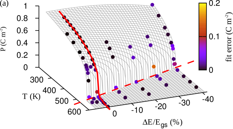
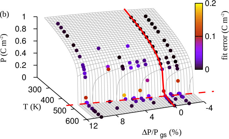
Figure 3: (Color online) Computed $P(T)$ curves for a variety of “(Ti–O)⁴” modified models. Panel (a): Models in which $E_{gs}$ changes while $P_{gs}=P_{gs}^{0}$ is kept constant. Panel (b): Models in which $P_{gs}$ changes while $E_{gs}=E_{gs}^{0}$ is kept constant.

This apparent failure of the mean-field prediction is shocking, as previous works on related models suggest that such an approximation should be able to capture the main qualitative behaviors of our PTO potential.Lines (1969); Pytte and Feder (1969); Waghmare and Rabe (1997) Let us consider in some detail such a discrepancy. Manipulating the 2nd- and 4th-order Ti–O couplings in our PTO model may seem equivalent to tuning the parameters $A$ and $B$ in $\phi^{4}$ Hamiltonian [Eq. (1)]. An important difference, though, is that such a modification of our potential involves changes in the dispersion of the phonon bands. For example, Table 1 gives information about a couple of constant-$E_{gs}^{0}$ models that present different $P_{gs}$ values [see potentials labeled “(Ti–O)⁴”, where the notation indicates the highest-order coupling that was modified to construct them]. The $C_{\rm FE}$ parameter given in the Table quantifies the curvature at $\Gamma$ of the bands associated with the FE instability [see Fig. 1(b)], and is analogous to the $C$ parameter of the $\phi^{4}$ Hamiltonian. Interestingly, in our constant-$E_{gs}^{0}$ models, larger $P_{gs}$ values correspond to smaller $C_{\rm FE}$ curvatures, and smaller $C_{\rm FE}$’s are consistent with the observed decrease in $T_{\rm C}$ according to Eq. (3). Thus, a reduction in $T_{\rm C}$ for increasing $P_{gs}$ does not necessarily imply the failure of Eq. (3).

We were able to specifically confirm the influence of $C_{\rm FE}$ on the obtained $T_{\rm C}$’s. To do so, we constructed models in which $C_{\rm FE}$ was modified while keeping $E_{gs}=E_{gs}^{0}$ and $P_{gs}=P_{gs}^{0}$ constant, which required the introduction of an additional harmonic coupling between neighboring Ti atoms (see sketch in Fig. 2). Table 1 shows the results for two representative cases, labeled “(Ti–Ti)²”. The observed behavior makes good physical sense: A larger $C_{\rm FE}$ implies a greater energy cost for the occurrence of inhomogeneous locally-polar distortions that are mutually exclusive with the dominant FE soft mode, and hence results in a higher $T_{\rm C}$. Additionally, we can numerically evaluate Eq. (3) using the information in Table 1 for the “(Ti–O)⁴” models with constant $E_{gs}^{0}$. Thus, for example, Eq. (3) predicts that our model with $P_{gs}/P^{0}_{gs}$ = 1.10 and $C_{\rm FE}/C_{\rm FE}^{0}$ = 0.92 should present an enhancement of about 11% in $T_{\rm C}$; however, such a prediction is in obvious disagreement with the computed decrease.

Interestingly, it may seem that our data suggest an alternative predictor for $T_{\rm C}$. For the models in Table 1, we report the curvature of the $E(P)$ curve at $P=0$ [$E^{\prime\prime}(0)$ or $A_{\rm FE}$ in Fig. 1(a)], which essentially corresponds to the parameter $A$ of the $\phi^{4}$ Hamiltonian. This parameter measures how unstable the $P=0$ paraelectric (PE) state is: large negative values of $A_{\rm FE}$ imply a greater difficulty to stabilize the PE phase, and should thus correspond to higher $T_{\rm C}$’s. Hence, one may heuristically propose $T_{\rm C}\sim|A_{\rm FE}|$, which is essentially satisfied by all the models we studied. It is worth noting that, in the case of the “(Ti–O)⁴” models in which we vary the ground state polarization at constant $E_{gs}^{0}$, changes in $P_{gs}$ and $|A_{\rm FE}|$ are forcefully correlated, an increase of the former implying a decrease of the latter. Hence, the $T_{\rm C}\sim|A_{\rm FE}|$ and $T_{\rm C}\sim P_{gs}^{2}$ rules are incompatible in this case, and we find that the former matches our Monte Carlo results better. We further investigated the validity of this new rule by considering other modified models (not shown here). Ultimately, we found that, in the constant-$E_{gs}^{0}$ “(Ti–O)⁴” cases of Table 1, we should attribute the changes in transition temperature to the variations in the $C_{\rm FE}$ parameter rather than to changes in $A_{\rm FE}$. Nevertheless, we did obtain additional indications of the importance of the details of the $E(P)$ curve from our last set of modified models, which we describe in the following.

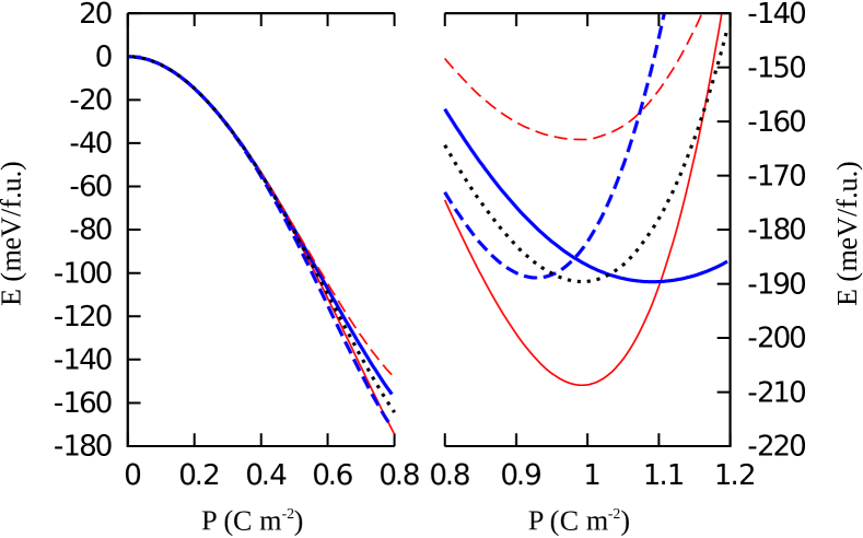
Figure 4: (Color online) Comparison of the double-well potential for the FE instability of PTO corresponding to our reference model (black dotted line) and the “(Ti–O)⁸” modified potentials described in the text. Red and blue lines correspond to constant-$P_{gs}$ and constant-$E_{gs}$ models, respectively. These $E(P)$ curves were obtained by determining, for each $P$ value, the structure that minimizes the energy and can be described with a 5-atom unit cell.

Finally, we constructed models in which only $E_{gs}$ or $P_{gs}$ vary while the other parameters discussed so far ($C_{\rm FE}$ and $A_{\rm FE}$) are kept fixed. Doing this required the tuning of Ti–O couplings up to 8th-order while keeping the harmonic interactions constant; these models are labeled “(Ti–O)⁸” in Table 1. Our results ratify that $E_{gs}$ has a considerable impact on $T_{\rm C}$, in qualitative agreement with Eq. (2). We also find that varying $P_{gs}$ alone has an effect on $T_{\rm C}$. However, once again we observe that a larger ground state distortion leads to a smaller transition temperature, in disagreement with initial expectations.

When we examined this last set of modified models, we observed that a larger $P_{gs}$ value corresponds to a shallower energy surface around the FE minimum (see Fig. 4). In view of this, we reexamined all our potentials and found that the curvature at $P=P_{gs}$, which we call $A^{\prime}$ in Table I, does correlate with the computed transition temperatures. We might thus speculate that, generally speaking, stiffer FE phases (with larger $A^{\prime}$ values associated to them) will be more difficult to destabilize, and will thus correspond to higher $T_{\rm C}$’s. This observation suggests yet another heuristic predictor for the transition temperature, namely, $T_{\rm C}\sim A^{\prime}$. It is interesting to note that for the $\phi^{4}$ potential we have $A^{\prime}=-2A$; hence, in this case we can write $T_{\rm C}\sim A^{\prime}\sim|A|$, which coincides with the above mentioned predictor based on curvature of $E(P)$ around $P=0$.

A natural next step would be to investigate models in which we would keep all the parameters in Table I constant except for $E_{gs}$ or $P_{gs}$. This would require our introducing couplings of even higher order, and producing ever more artificial potentials. Hence, we did not pursue this line any further.

III Discussion

In view of these results, what is the status of the predictors for $T_{\rm C}$ mentioned in the introduction? Are our findings compatible with existing literature? What are the lessons to be learned?

III.1 Implications for $T_{\rm C}$ predictors

We have found that the mean-field result for the $\phi^{4}$ model [Eq. (3)], which is essentially equivalent to the formulas proposed by a number of authors,Lines (1969); Pytte and Feder (1969) does not give an accurate description of the behavior of our simulated materials. The main conflict concerns the qualitative dependence of $T_{\rm C}$ on $P_{gs}^{2}$, as we have found that our simulations render a behavior ($T_{\rm C}$ decreases with growing $P_{gs}^{2}$) that is just opposed to the expected one. This is a serious discrepancy, as the $\phi^{4}$ model can be seen as a simplified version of our PTO potential, and we certainly expect its behavior to be qualitatively well captured by the mean-field approximation. Hence, how can we explain this apparent contradiction?

Let us begin by noting that, while we are in principle entitled to associate parameters in the $\phi^{4}$ model with the analogous quantities for our PTO potential, this correspondence is not a strict one. The $\phi^{4}$ model has only three independent constants – which we can choose to be $A$, $B$, and $C$ in Eq. (1) – and, once those are given, we can write simple relationships between the derived quantities. Thus, for example, the equality $u_{gs}^{2}=4E_{gs}/A$ is always fulfilled by the $\phi^{4}$ potential. However, as one can easily check from the information in Table 1, the analogous identity $P_{gs}^{2}=\gamma E_{gs}/A_{\rm FE}$, where $\gamma$ is an appropriate constant, does not hold for our PTO potentials. For example, for the model described in the second line of Table 1 we have $(P_{gs}/P_{gs}^{0})^{2}=1$, which differs a lot from $E_{gs}/E_{gs}^{0}\times A_{\rm FE}^{0}/A_{\rm FE}=0.63$. It is thus obvious that the relationships that are valid for the $\phi^{4}$ model, even the simplest ones pertaining to the ground state properties and potential shape, do not necessarily apply to more realistic models of structural transitions.

The reason for such differences lies on the inherent complexity of our reference PTO potential. Indeed, even for a 4th-order model like ours, the energy well corresponding to the FE instability can effectively be of a higher polynomial order due to the anharmonic couplings between the unstable FE mode and other modes and strains in the material. This is a critical difference with respect to the $\phi^{4}$ model, and the likely cause of the discrepancies mentioned above. To understand this better, consider the energy of a simple model

$$E=au^{2}+bu^{4}+cv^{2}+dv^{4}+evu^{3}\,,$$ (5)

where $u$ is the amplitude of a soft mode with an associated double-well potential ($a<0$, $b>0$) and $v$ is the amplitude of a stable mode ($c,d>0$) coupled with $u$ anharmonically. In such a case, it is easy to see that, upon condensation of $u\neq 0$, we get a secondary distortion

$$v=-\frac{e}{2c}u^{3}\,,$$ (6)

where, for simplicity, to derive this expression we have assumed that $v$ will always be relatively small. By substituting Eq. (6) into Eq. (5) we get a renormalized energy for $u$ that reads

$$E^{\prime}=au^{2}+bu^{4}-\frac{e^{2}}{4c}u^{6}+\frac{de^{4}}{16c^{4}}u^{12}\,,$$ (7)

which is effectively of 12th order. [The ${\cal O}(v^{4})$ term that eventually leads to the ${\cal O}(u^{12})$ contribution has been included here to make it clear that the renormalized energy continues to be bounded from below, despite the ${\cal O}(u^{6})$ term being negative.] This example constitutes a realistic description of how the FE soft mode ($u$) and other $\Gamma$-point modes with the same polar symmetry ($v$) interact anharmonically. Such couplings are responsible for a variety of effects in PTO, such as the significant differences that exist between the atomic displacements corresponding to the FE ground state and those associated with the eigenvector of the FE soft mode of the cubic phase, etc. The precise list of anharmonic couplings in our PTO potential can be found in Table 1 of Ref. Wojdeł et al., 2013.

It is clear that our model for PTO is closer to reality than the simple $\phi^{4}$ Hamiltonian. Hence, one may wonder: do our results imply that the $T_{\rm C}\sim Cu_{gs}^{2}$ rule should not be able to describe real materials? To answer this question, let us note that the modified models considered in this work correspond to somewhat artificial situations in which changes in $P_{gs}$ and $E_{gs}$ are strictly decoupled. In contrast, in reality one expects strong soft mode instabilities to involve large values of both $|E_{gs}|$ and $P_{gs}$. (This is indeed what we obtain for our PTO model when we simply crank up the magnitude of the interactions responsible for the FE instability without imposing any constraint.) Hence, leaving aside unusual choices of potential parameters, we can generally expect $|u_{gs}|^{n}\sim|E_{gs}|^{m}\sim s$, where $s$ measures the strength of the structural instability, and $n$ and $m$ are two positive numbers. In other words, in general we expect $u_{gs}^{2}$ and $|E_{gs}|$ to be essentially equivalent as $T_{\rm C}$ predictors.

Now, even though they may correspond to unusual situations, the unexpected results that we obtained for our modified models with constant-$E_{gs}^{0}$ do suggest some relevant conclusions. As mentioned above, when subject to the constant-$E_{gs}^{0}$ constraint, an increase of $P_{gs}$ involves changes in the potential surface (e.g., around $P=0$ and/or $P=P_{gs}$) that tend to result in a lower $T_{\rm C}$. This finding indicates that: (1) Subtle changes in the potential surface can have an important impact on the computed transition temperature. As far as we know, this is an effect that had not been noticed before, and one that is important to keep in mind if we want to construct first-principles model potentials (like those of Ref. Wojdeł et al., 2013 and othersZhong et al. (1994); Shin et al. (2005); Sepliarsky et al. (2005)) that render accurate transition temperatures. (2) The fundamental quantities for predicting $T_{\rm C}$ are those directly related to the energy. Thus, our results suggest that $P_{gs}^{2}$ or $u_{gs}^{2}$ may act as predictors only because their magnitude is usually connected with the strength of the structural instability. In contrast, $|E_{gs}|$ is a fundamentally more robust predictor for $T_{\rm C}$.

Of course, the above arguments imply that, in our opinion, our results are perfectly compatible with the empirical rule $T_{\rm C}\sim u_{gs}^{2}$ proposed by Abrahams et al.Abrahams et al. (1968) In fact, it is worth mentioning that, when discussing the physical interpretation of their newly-found law, these authors viewed the value of $u_{gs}^{2}$ as a measure of the “thermal energy at the Curie point”. We believe that such an interpretation is the most natural one, and it falls in line with our conclusions.

Finally, let us note that we numerically fitted our results for $T_{\rm C}$ using an expression of the form

$$\begin{split}\frac{T_{\rm C}}{T_{\rm C}^{0}}=&\left(\frac{E_{gs}}{E_{gs}^{0}}\right)^{n_{1}}\times\left(\frac{P_{gs}}{P_{gs}^{0}}\right)^{n_{2}}\times\left(\frac{C_{\rm FE}}{C_{\rm FE}^{0}}\right)^{n_{3}}\\ &\times\left(\frac{A_{\rm FE}}{A_{\rm FE}^{0}}\right)^{n_{4}}\times\left(\frac{A^{\prime}}{A^{\prime 0}}\right)^{n_{5}}\,,\end{split}$$ (8)

where the exponents are adjustable real numbers. This exercise showed that the $A_{\rm FE}$ and $A^{\prime}$ parameters are comparatively unimportant for determining $T_{\rm C}$, and can be neglected in a first approximation. Further, we obtained $n_{1}=0.49$ for $E_{gs}$, $n_{2}=-0.34$ for $P_{gs}$, and $n_{3}=0.29$ for $C_{\rm FE}$, reflecting the dominant role of the energy difference between the high- and low-symmetry structures. As expected from our results summarized in Table I, the magnitude of $P_{gs}$ is found to be inversely proportional to $T_{\rm C}$. At the same time, in typical cases in which $E_{gs}$ and $P_{gs}$ are correlated and grow/decrease together, we can expect the $E_{gs}/E_{gs}^{0}$ term to dominate.

III.2 Non-trivial cases: competing instabilities

Let us now comment on the related works of Grinberg and RappeGrinberg and Rappe (2004) and Juhas et al.,Juhas et al. (2004) who combined first-principles results and experimental information to empirically identify predictors for $T_{\rm C}$. These authors studied a number of complex solid solutions involving PbTiO₃ and PbZrO₃ crystals mixed with partly-disordered perovskites PbMg_1/3Nb_2/3O₃, PbZn_1/3Nb_2/3O₃, and PbSc_2/3W_1/3O₃. Experimentally, these materials are found to behave as relaxor ferroelectrics, with the temperature $T_{\epsilon,{\rm max}}$ – corresponding to the maximum dielectric response – being the closest analogue of the Curie point of a normal ferroelectric. By comparing the experimental values for $T_{\epsilon,{\rm max}}$ with the computed $u_{gs}$ ($u_{gs}$ quantifies a local symmetry-breaking distortion in this case), a good correlation of the form $T_{\epsilon,{\rm max}}\sim u_{gs}^{2}$ was observed. At first sight, this finding seems to ratify the conclusions of Abrahams et al.,Abrahams et al. (1968) and seems perfectly compatible with the above discussion of our results. However, the authors of Ref. Juhas et al., 2004 also observed clear deviations from the $T_{\epsilon,{\rm max}}\sim|E_{gs}|$ rule that would be analogous to Eq. (2). How does this affect our conclusion that $|E_{gs}|$ is the more fundamental and robust predictor for $T_{\rm C}$?

A careful inspection of the data in Ref. Juhas et al., 2004 (see e.g. Table IV in that paper) suggests that there are subtleties hiding behind the proposed $T_{\epsilon,{\rm max}}\sim u_{gs}^{2}$ rule. As expected for Pb-based ferroelectrics and relaxors, Juhas et al. found that the distortions characterizing the low-symmetry phases are dominated by the off-centering of the Pb atoms, with the displacements of the $B$-site cations (Ti, Zr, etc.) being smaller by a factor of 2 or 3, typically. However, their results also show that the magnitude of the Pb displacements does not correlate well with $T_{\epsilon,{\rm max}}$. Instead, their data suggest that what correlates strongly with $T_{\epsilon,{\rm max}}$ is the displacement of the $B$-site cations, and it is such a correlation what ultimately justifies the $T_{\epsilon,{\rm max}}\sim u_{gs}^{2}$ rule. (The precise relationship was obtained as the result of a fitting procedure in which the contributions from the Pb and $B$-atom displacements were considered separately.Juhas et al. (2004)) Such an atomistic foundation for the $u_{gs}^{2}$ predictor, with the relatively small displacements of the $B$-cations dominating the effect, is truly intriguing.

Interestingly, when discussing their $T_{\epsilon,{\rm max}}\sim u_{gs}^{2}$ rule, Juhas et al. wrote that the change in $T_{\epsilon,{\rm max}}$ is not “directly caused by changes in the structural features such as the cation shifts, but is due to the changes in the energetics of competing instabilities”. This is a subtle point that is worth discussing. The competing instabilities mentioned by these authors are the local polar distortions (which ultimately prevail) and the so-called anti-ferrodistortive (AFD) modes involving concerted rotations of the oxygen octahedra in the perovskite structure. We have recent and clear evidence that this kind of competition has a large effect on the Curie temperature of PTOWojdeł et al. (2013) and related materials.Kornev et al. (2006) In particular, as shown in Ref. Wojdeł et al., 2013 for the case of our PTO model, it is possible to modify the energetics of the oxygen-octahedra rotations (e.g., artificially suppressing them) and obtain an effect in $T_{\rm C}$ (a very large increase), even if all the key parameters describing the FE instability and ground state ($E_{gs}$, $P_{gs}$, $C_{\rm FE}$, $A_{\rm FE}$, and $A^{\prime}$) remain constant. Hence, a priori there is no reason to expect the above mentioned $T_{\rm C}$ predictors to describe well the behavior of materials in which this type of hidden effects are important. In fact, it seems natural to suspect that departures from the normal behavior may indicate the presence of this kind of phenomena.

One can thus conjecture that, in the cases considered in Refs. Grinberg and Rappe, 2004 and Juhas et al., 2004, larger displacements of the $B$-site cations probably correspond to weaker AFD instabilities, which would in turn result in a less important competition and a higher $T_{\epsilon,{\rm max}}$. Note that this connection is not inconsistent with the observation that, in the AFD-dominated phases of many perovskite oxides, the $B$-site cations usually stay at the center of O₆ octahedra. This tendency can be explained by the size effects captured by the so-called tolerance factor.Davies et al. (2008); Fornari and Singh (2001); Reaney et al. (1994)

It thus seems that the simple-looking predictor for $T_{\epsilon,{\rm max}}$ proposed in Refs. Grinberg and Rappe, 2004; Juhas et al., 2004 hides rather complex structural and lattice-dynamical mechanisms behind it. As just mentioned, in these Pb-based relaxors $u_{gs}^{2}$ seems to (anti)correlate with the importance of the FE–AFD competition, which in turn controls the ordering temperature. In contrast, due to the structural complexity of these materials, $u_{gs}^{2}$ does not correlate well with the depth of the potential energy wells. In view of this, the results of Refs. Grinberg and Rappe, 2004; Juhas et al., 2004 cannot be taken as support for the conclusions of Abrahams et al.,Abrahams et al. (1968) which rely on the connection between $u_{gs}$ and $E_{gs}$ as emphasized above. Nevertheless, such results do show that, even in difficult cases involving competing instabilities, it may be possible to find predictors for $T_{\rm C}$ associated with simple properties of the ground state. The possibility of extending such a conclusion to other materials with competing instabilities remains to be confirmed.

III.3 Additional remarks

Abrahams et al.Abrahams et al. (1968) noted that the validity of their simple empirical rule implies that very different materials must present similar properties of some sort. Indeed, as discussed theoretically by Lines,Lines (1969); Lines and Glass (1977) the applicability of Eq. (4) to a set of diverse ferroelectrics indicates that there exists an effective force constant (in essence, this would be the proportionality constant between $T_{\rm C}$ and $u_{gs}^{2}$) that (1) is probably dominated by long-range dipole-dipole interactions and (2) is quantitatively similar for all the materials considered in Ref. Abrahams et al., 1968. This interpretation is consistent with our results: We have found that variations in $C_{\rm FE}$ have a large impact on $T_{\rm C}$; hence, if a $T_{\rm C}$ predictor that disregards such variations applies to a set of materials, it follows that $C_{\rm FE}$ must be similar for all of them. We believe that, as long as we are dealing with simple cases (e.g., in absence of a materials-dependent competition between structural instabilities), such reasonings probably apply. Yet, in view of the above-described subtleties associated with the Pb-based relaxors, it is legitimate to wonder how many intricate and material-specific behaviors are hiding behind the result of Abrahams et al., and how much their empirical rule really tells us about the nature of the interatomic interactions in each of the specific compounds they considered.

In the same spirit, Grinberg and RappeGrinberg and Rappe (2004) suggested that the PTO-based solid solutions they investigated must present somewhat similar Landau potentials. More specifically, they worked with a Landau energy of the form

$$F=\alpha(T-T_{\rm C})P^{2}+\beta P^{4}\,,$$ (9)

with $\alpha,\beta>0$, to justify the relationship

$$T_{\rm C}=2\beta P_{gs}^{2}/\alpha\,,$$ (10)

and inferred that the compounds they studied (for which $T_{\rm C}/P_{gs}^{2}$ is approximately constant) must present comparable $\beta/\alpha$ ratios. This is a tempting interpretation that seems to give us some physical insight into the energetics of the polar instabilities in these materials. However, noting that the findings of these authors on Pb-based relaxors probably rely on subtle effects involving competing instabilities, and that such effects cannot be modeled within a simple Landau scheme, we should be careful to avoid overinterpreting such observations.

Finally, let us note that we have limited our discussion to $T_{\rm C}$ predictors that have a clear justification, may it be empirical, theoretical, or heuristic. We have purposely avoided the consideration of other possibilities with a less clear basis. For example, it may be tempting to consider the Landau potential of Eq. (9) and derive possible rules like $T_{\rm C}=2\beta P_{gs}^{2}/\alpha$ [Eq. (10)] or $T_{\rm C}^{2}=4\beta|E_{gs}|/\alpha^{2}$. However, while the former seems equivalent to Eq. (4) for $n=2$, and the latter may resemble Eq. (2), it must be emphasized that these identities cannot be used to justify a predictor for $T_{\rm C}$. The reason is that it is perfectly legitimate to choose $T_{\rm C}$, $P_{gs}$, and $E_{gs}$ as independent parameters of the Landau potential and, hence, no relationship among these quantities needs to hold. Note, for example, that in addition to the two expressions just mentioned, we may write others such as $T_{\rm C}=2|E_{gs}|/(\alpha P_{gs}^{2})$, which renders a very different and equally unjustified relationship between our properties of interest.

IV Conclusions

We have examined an effective model for PbTiO₃, a material with a representative soft mode-driven structural transition, to investigate which features of the potential control the transition temperature $T_{\rm C}$. Our main result is that $T_{\rm C}$ correlates strongly with the energy difference between the high-symmetry and low-symmetry structures ($E_{gs}$). In contrast, we find that the magnitude of the symmetry-breaking distortion ($u_{gs}$) is a less robust predictor, although it can be expected to work well in typical cases in which $|E_{gs}|$ and $|u_{gs}|$ are strongly correlated. Additionally, our results reveal the sizable impact that subtle features of the energy surface have on the computed $T_{\rm C}$, providing us with useful information for the construction of more accurate model potentials from first principles.

By comparing our results with existing literature, we can conclude that: (1) Whenever simple $T_{\rm C}$ predictors work well for a family of materials, this is indicative that the potentials of such compounds share some common features. This conclusion is in agreement with previous observations by other authors.Abrahams et al. (1968); Lines and Glass (1977) (2) Whenever the simple predictors fail, this suggests the occurrence of subtle structural and lattice-dynamical effects involving strong anharmonic interactions between modes.

We thus hope our results will bring new insights to the analysis of complex phase-transition and lattice-dynamical phenomena, and permit more effective computational works to design materials with tailored temperature-dependent properties.

This work was supported by MINECO-Spain (Grants No. MAT2010-18113 and No. CSD2007-00041) and CSIC [JAE-doc program (JCW)].

*

Appendix A Fitting the $P(T)$ curves

To analyze our data and determine $T_{\rm C}$ for each considered model in a robust and reliable way, we employed a fitting procedure that assumes a heuristic form for $P(T)$. More precisely, we used

$$P(T)=\left\{\begin{array}[]{ll}\mu(T_{\rm C}-T)^{\delta}&{\rm for}\;\;T<T_{\mathrm{C}}\\ 0&{\rm for}\;\;T>T_{\rm C}\\ \end{array}\;,\right.$$ (11)

which depends on the three free parameters $\mu$, $T_{\rm C}$, and $\delta$. This functional form is compatible with the description of a second order phase transition (which corresponds to $\delta=1/2$ within Landau theory), and is also flexible enough to capture more complex behaviors appearing when the transition is discontinuous. (We numerically found that $\delta\simeq 1/5$ reproduces well the results for our reference model, as well as the typical first-order transition described by a sixth-order Landau theory.) The good quality of the fits can be appreciated in Fig. 1(c), which shows a representative case.

Additionally, we introduced a linear dependence of the free parameters – $T_{\rm C}$, $\mu$, and $\delta$ – on the specific tuned properties (i.e., $E_{gs}/E^{0}_{gs}$ or $P_{gs}/P^{0}_{gs}$) to be able to plot the surfaces appearing in Fig. 3. There we also report the deviation (“fit error”) between the fitted curves and the computed polarization values, which turns out to be very small except in the immediate vicinity of $T_{\rm C}$.

References

- Blinc and Žekš (1974) R. Blinc and B. Žekš, Soft modes in ferroelectrics and antiferroelectrics, Selected Topics in Solid State Physics (North-Holland Pub. Co., 1974).
- Dove (2005) M. T. Dove, Introduction to Lattice Dynamics, Cambridge Topics in Mineral Physics and Chemistry (Cambridge University Press, 2005).
- Wojdeł and Íñiguez (2010) J. C. Wojdeł and J. Íñiguez, Physical Review Letters 105, 037208 (2010).
- Bruce (1980) A. D. Bruce, Advances in Physics 29, 111 (1980).
- Abrahams et al. (1968) S. C. Abrahams, S. K. Kurtz, and P. B. Jamieson, Physical Review 172, 551 (1968).
- Lines (1969) M. E. Lines, Physical Review 177, 797 (1969).
- Lines and Glass (1977) M. E. Lines and A. M. Glass, Principles and Applications of Ferroelectrics and Related Materials, Oxford Classic Texts in the Physical Sciences (Clarendon Press, 1977).
- Grinberg and Rappe (2004) I. Grinberg and A. M. Rappe, Physical Review B 70, 220101 (2004).
- Juhas et al. (2004) P. Juhas, I. Grinberg, A. M. Rappe, W. Dmowski, T. Egami, and P. K. Davies, Physical Review B 69, 214101 (2004).
- Wojdeł et al. (2013) J. C. Wojdeł, P. Hermet, M. P. Ljungberg, P. Ghosez, and J. Íñiguez, Journal of Physics: Condensed Matter 25, 305401 (2013).
- (11) For a discussion of the discrepancy between the predicted temperature and the experimental result (about 760 K), see Ref. Wojdeł et al., 2013.
- (12) The computed hysteresis is expected to depend strongly on the size of the simulated supercell. In our case, the supercell is probably too small to render a realistic description of the hystereis in the ferroelectric transition of PTO, as we get a very small effect.
- Pytte and Feder (1969) E. Pytte and J. Feder, Physical Review 187, 1077 (1969).
- Waghmare and Rabe (1997) U. V. Waghmare and K. M. Rabe, Physical Review B 55, 6161 (1997).
- Zhong et al. (1994) W. Zhong, D. Vanderbilt, and K. M. Rabe, Physical Review Letters 73, 1861 (1994).
- Shin et al. (2005) Y.-H. Shin, V. R. Cooper, I. Grinberg, and A. M. Rappe, Physical Review B 71, 054104 (2005).
- Sepliarsky et al. (2005) M. Sepliarsky, A. Asthagiri, S. R. Phillpot, M. G. Stachiotti, and R. L. Migoni, Current Opinion in Solid State and Materials Science 9, 107 (2005).
- Kornev et al. (2006) I. A. Kornev, L. Bellaiche, P.-E. Janolin, B. Dkhil, and E. Suard, Physical Review Letters 97, 157601 (2006).
- Davies et al. (2008) P. K. Davies, H. Wu, A. Y. Borisevich, I. E. Molodetsky, and L. Faber, Annual Review of Materials Research 38, 369 (2008).
- Fornari and Singh (2001) M. Fornari and D. J. Singh, Physical Review B 63, 092101 (2001).
- Reaney et al. (1994) I. M. Reaney, E. L. Colla, and N. Setter, Japanese Journal of Applied Physics 33, 3984 (1994).