Quantitative nonorientability of embedded cycles

Abstract.

We introduce an invariant linked to some foundational questions in geometric measure theory and provide bounds on this invariant by decomposing an arbitrary cycle into uniformly rectifiable pieces. Our invariant measures the difficulty of cutting a nonorientable closed manifold or mod-2 cycle in $\mathbb{R}^{n}$ into orientable pieces, and we use it to answer some simple but long-open questions on filling volumes and mod-$\nu$ currents.

1. Introduction

If $T$ is a Lipschitz curve in $\mathbb{R}^{N}$, there is a minimal surface $U$ whose boundary is $T$. If we trace $T$ twice to obtain a curve $2T$, there is a minimal surface $U^{\prime}$ whose boundary is $2T$. At first glance, one might guess that $U^{\prime}=2U$. This is easy to prove when $N=2$ and is a theorem of Federer [Fed75] when $N=3$, but remarkably, it is false when $N\geq 4$! L. C. Young constructed an example of a curve $T\colon S^{1}\to\mathbb{R}^{4}$ that lies on an embedded Klein bottle and a chain $U$ such that $U$ is a minimal filling of $T$, but $2U$ is not a minimal filling of $2T$. In fact, $\operatorname{mass}U^{\prime}$ is only about $1.5\operatorname{mass}U$ [You63].

A version of Young’s example is shown in Figure 1. Consider a Klein bottle $K$ embedded in $\mathbb{R}^{4}$ and draw $2k+1$ equally-spaced rings on $K$. Since these rings are drawn on a Klein bottle, we can orient them so that adjacent rings have “opposite” orientations. Let $T$ be the sum of these rings.

On one hand, we can fill $2T$ with a chain supported on $K$. Since the rings have alternating orientations, we can fill each pair of adjacent rings with a thin cylindrical band. The curves in $T$ cut $K$ into $2k+1$ bands, and if we give these bands alternating orientations, their boundary is $2T$ (right side of Fig. 1). When $k$ is large, this is nearly optimal and has mass roughly $\operatorname{area}{K}$.

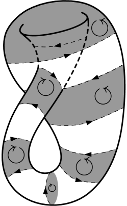
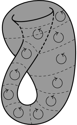
$T$	A filling of $T$	A filling of $2T$

Figure 1. Fillings of a 1-cycle on a Klein bottle. The 1-cycle $T$ consists of $2k+1$ loops with alternating orientations. In the middle, we fill $T$ with $k$ cylindrical bands and a disc, and on the right, we fill $2T$ with $2k+1$ cylindrical bands with alternating orientations.

On the other hand, we cannot use the same technique to fill $T$. Since there’s an odd number of rings in $T$, we can fill all but one of the rings using $k$ bands, but we need to fill the last ring with a disc (middle of Fig. 1). When $k$ is large, a filling like this is nearly optimal and has area roughly $(\operatorname{area}{K})/2$ plus the area of the extra disc — well over half the area of a minimal filling of $2T$.

Questions in geometric measure theory related to this example and examples with different multipliers found by Morgan [Mor84] and White [Whi84] have been open almost since Federer and Fleming’s first papers developing normal and integral currents. Because of these examples, the flat distance

(1) $$\mathcal{F}(A)=\inf\{\operatorname{mass}R+\operatorname{mass}S\mid A=R+\partial S,R\in\mathcal{R}_{d}(\mathbb{R}^{N}),S\in\mathcal{R}_{d+1}(\mathbb{R}^{N})\}.$$

is not a norm; if $T$ is as above, then we may have $\mathcal{F}(\nu T)<\nu\mathcal{F}(T)$. Consequently, several basic questions have remained unanswered, including:

1. If $\nu>0$ is a positive integer and $\mathcal{F}_{d}(\mathbb{R}^{N})$ is the space of integral flat $d$–chains in $\mathbb{R}^{N}$, is the multiply-by-$\nu$ map $f\colon\mathcal{F}_{d}(\mathbb{R}^{N})\to\mathcal{F}_{d}(\mathbb{R}^{N})$, $f(T)=\nu T$ an embedding?

2. Is the set of flat chains modulo $\nu$ a quotient of the integral flat chains?

3. We can define a real flat norm by replacing the rectifiable currents in (1) by normal currents. How is the real flat norm related to the flat distance?

In this paper, we will relate the first two of these questions to the geometry of nonorientable cycles in $\mathbb{R}^{N}$ and answer both of them positively (Corollaries 1.4 and 1.5).

Specifically, we will define the following invariant. If $A$ is a mod–$\nu$ cycle in $\mathbb{R}^{N}$ (a Lipschitz cycle or integral current modulo $\nu$) and $R$ is a $\mathbb{Z}$–cycle (Lipschitz cycle or integral current) such that $A\equiv R\pmod{\nu}$, we say that $R$ is a pseudo-orientation of $A$. Let the nonorientability of $A$ be

$$\operatorname{NO}(A)=\inf\{\operatorname{mass}R\mid\text{$R$ is a pseudo-orientation of $A$}\}.$$

Any smooth submanifold of $\mathbb{R}^{N}$ has a pseudo-orientation. For example, suppose that $M$ is a nonorientable genus-$g$ surface smoothly embedded in $\mathbb{R}^{N}$ and that $A=[M]$ is the fundamental class of $M$. This is a cycle with $\mathbb{Z}_{2}$ coefficients, but we can lift it to a cycle with integer coefficients by cutting $M$ into orientable pieces. Let $\Gamma$ be a smooth graph embedded in $M$ whose complement consists of orientable pieces $M_{1},\dots,M_{n}$. We choose orientations on the $M_{i}$ arbitrarily to get fundamental classes $[M_{1}],\dots,[M_{n}]$. Then $R_{0}:=\sum[M_{i}]$ is a 2–chain over $\mathbb{Z}$ and $\operatorname{supp}\partial R_{0}\subset\Gamma$. Each edge of $\Gamma$ occurs in $\partial R_{0}$ with coefficient 0 or $\pm 2$, depending on the orientations of the neighboring regions in $M$. Let $R_{1}$ be a chain with integer coefficients such that $\partial R_{1}=\partial R_{0}/2$ and define $R=R_{0}+2R_{1}$. Then

$$R\equiv\sum[M_{i}]\equiv[M]\pmod{2},$$

so $R$ is a pseudo-orientation of $[M]$. The mass of $R$, however, could be much larger than the area of $M$, especially if $M$ is very complicated.

In this paper, we will show that the nonorientability of a cycle is bounded by its mass:

Theorem 1.1.

For every $\nu,d,N>0$, there is a $c>0$ such that

$$\operatorname{NO}(A)\leq c\operatorname{mass}A$$

for every $A\in\mathbf{I}^{\nu}_{d}(\mathbb{R}^{N})$ with $\partial A=0$.

Here, $\mathbf{I}^{\nu}_{d}(\mathbb{R}^{N})$ is the set of integral currents modulo $\nu$; when $\nu>0$, $\nu\in\mathbb{Z}$, the integral currents modulo $\nu$ are a chain complex that contains the mod-$\nu$ polyhedral chains as a dense subset.

Note that it is not clear a priori that every integral current mod $\nu$ with no boundary has a pseudo-orientation. Federer [Fed69, 4.2.26] asserted that there are integral currents modulo $2$ that do not lift to integral currents, though his example, an infinite sum of projective planes with finite total mass, turns out to have an error (see [Pau77, 2.5]).

The theorem will follow from the following statement about cycles in the unit grid in $\mathbb{R}^{N}$

Theorem 1.2.

For every $\nu,d,N>0$, there is a $c>0$ such that if $A\in C_{d}(\tau;\mathbb{Z}_{\nu})$ is a mod-$\nu$ cellular cycle in the unit grid in $\mathbb{R}^{N}$, then there is a cellular cycle $R\in C_{d}(\tau;\mathbb{Z})$ such that $A\equiv R\pmod{\nu}$ and $\operatorname{mass}R\leq c\operatorname{mass}A$. It follows that

$$\operatorname{NO}(A)\leq c\operatorname{mass}A.$$

(Indeed, though several of our applications will involve integral currents and flat chains, our use of currents will be restricted to the proofs of those applications, and the proof of Theorem 1.2 can be read without previous familiarity with currents.)

The main difficulty in proving Theorem 1.2 is dealing with cycles that have complex topology at many scales and many locations. For example, consider the following sequence of surfaces: Let $C_{0}$ be the 2-dimensional surface of a unit 3-cube embedded in $\mathbb{R}^{4}$. The surface $C_{0}$ is orientable, but we can make it nonorientable by gluing crosscaps to its faces. Let $\Sigma$ be a crosscap consisting of a union of faces in the unit grid, with boundary a square of side length 10. We can partition $C_{0}$ into $6$ unit squares and construct $C_{1}$ by replacing each square by a scaled copy of $\Sigma$.

Then $C_{1}$ is a surface in the grid of side length $10^{-1}$, homeomorphic to a connected sum of six projective planes. Its fundamental class is a mod-2 cycle, and any pseudo-orientation of $C_{1}$ must cut through each crosscap, so $\operatorname{NO}([C_{1}])\sim 1$.

There are no large faces in $C_{1}$ to replace by crosscaps, but we can still add nonorientability at smaller scales by replacing smaller faces in $C_{1}$ by smaller crosscaps. Choose $100$ faces of $C_{1}$ of side length $10^{-1}$ and replace them by scaled copies of $\Sigma$ to obtain $C_{2}$. Each new crosscap contributes roughly $10^{-2}$ to the nonorientability, so in total, they contribute roughly $1$.

Proceeding inductively, we replace $100^{i}$ faces of $C_{i}$ of side length $10^{-i}$ to obtain $C_{i+1}$. A pseudo-orientation of $C_{k}$ must cut through all of the crosscaps at every scale, so

$$\operatorname{NO}([C_{k}])\sim\sum_{i=0}^{k-1}100^{i}10^{-2i}=k.$$

This is much larger than the area of the surface we started with. The only reason that this does not contradict Theorem 1.1 is that each added crosscap of diameter $r$ also increases the area of the surface by roughly $r^{2}$, so

$$\operatorname{area}(C_{k})\sim 1+\sum_{i=0}^{k-1}100^{i}10^{-2i}\sim k+1.$$

One can also imagine more complicated versions of $C_{k}$ using different scale factors or replacing squares by more complicated surfaces. Theorem 1.1 implies that in all such constructions, the extra nonorientability coming from replacing a square by a surface is bounded by the added area. Nevertheless, we conjecture that the ratio $\frac{\operatorname{NO}(A)}{\operatorname{mass}A}$ approaches its supremum for a sequence of self-similar surfaces like the $C_{i}$.

A remarkable feature of Theorem 1.1 is that it gives a bound that is independent of the topology of $A$; many related bounds depend on the topology. If $d=2$ and $A$ is the fundamental class of a surface $M\subset\mathbb{R}^{N}$, then bounds on the nonorientability of $[M]$ are related to bounds on systoles of $M$, which typically depend on the genus of $M$.

For example, as noted above, the nonorientability of $M$ is related to the difficulty of partitioning $M$ into orientable pieces. By choosing an orientation on each piece, one can lift such a partition to a partition of the double cover $\tilde{M}$ into two pieces of equal area. Cheeger’s inequality implies that there are surfaces (scalings of arithmetic hyperbolic surfaces) with unit area and genus $g$ such that any curve or set of curves that cuts the surface into two equal pieces has length at least $\sqrt{g}$. Similarly, one way to obtain a graph $\Gamma$ in $M$ whose complement consists of orientable pieces is to let $\Gamma$ be a pants decomposition of $M$. In a paper with Larry Guth and Hugo Parlier [GPY11], we showed that every pants decomposition of a “random” genus $g$ surface of area 1 has total length at least $g^{2/3-\epsilon}$.

This could suggest that some of the unusual geometric properties (large systoles, expander-type properties, large pants decompositions, etc.) that occur in arithmetic hyperbolic surfaces and random surfaces may not occur in surfaces that embed bilipschitzly (with respect to the euclidean metric, not in the sense of Nash) in $\mathbb{R}^{N}$. It would be interesting to know if this is the case.

1.1. Applications

Theorem 1.1 has several applications in geometric measure theory and the study of currents. First, Theorem 1.1 provides an answer to a question of L. C. Young. Let us define the filling volume $\operatorname{FV}(T)$ of a Lipschitz $d$-cycle $T\in C^{\mathrm{Lip}}_{d}(\mathbb{R}^{N})$ with $\partial T=0$ to be the infimal mass of a Lipschitz $(d+1)$–chain $U\in C^{\mathrm{Lip}}_{d+1}(\mathbb{R}^{N})$ such that $\partial U=T$. It follows from Theorem 1.1 that:

Corollary 1.3.

For any $d,N,\nu>0$, there is a $c>0$ such that for any $d$–cycle $T\in C^{\mathrm{Lip}}_{d}(\mathbb{R}^{N})$,

$$\operatorname{FV}(T)\leq c\operatorname{FV}(\nu T).$$

The behavior of $c$ when $\nu$ is large is an open and interesting question, because the limit $\lim_{\nu\to\infty}\frac{\operatorname{FV}(\nu T)}{\nu}$ is equal to the real filling volume $\operatorname{FV}_{\mathbb{R}}(T)$ of $T$. The real filling volume is the infimal mass of a Lipschitz $(d+1)$–chain $U\in C^{\mathrm{Lip}}_{d+1}(\mathbb{R}^{N};\mathbb{R})$ with real coefficients such that $\partial U=T$. L. C. Young’s example shows that the integral and real filling volumes of a cycle can be different, but it is unknown whether the ratio of these filling volumes is bounded.

The theorem also answers some questions about integral currents and flat chains that have been open since the 1960’s. In particular, the following corollaries answer a question in 4.2.26 of [Fed69] and part of a cluster of related questions studied by Almgren [Whi98].

Corollary 1.4.

Let $d,n,\nu\in\mathbb{N}$. The multiply-by-$\nu$ map $f\colon\mathcal{F}_{d}(\mathbb{R}^{N})\to\mathcal{F}_{d}(\mathbb{R}^{N})$, $f(T)=\nu T$ is an embedding, and the images $\nu\mathcal{F}_{d}(\mathbb{R}^{N})$ and $\nu\mathbf{I}_{d}(\mathbb{R}^{N})$ are closed.

and

Corollary 1.5.

If $T\in\mathbf{I}^{\nu}_{d}(\mathbb{R}^{N})$ is an integral current mod $\nu$, then $T\equiv T_{\mathbb{Z}}\pmod{\nu}$ for some integral current $T_{\mathbb{Z}}$.

These corollaries answer a question in 4.2.26 of [Fed69] and

Corollary 1.5 is somewhat subtle because of the terminology used to describe currents mod $\nu$. One can define quotients $\mathcal{F}_{d}(\mathbb{R}^{N})/\nu\mathcal{F}_{d}(\mathbb{R}^{N})$ and $\mathbf{I}_{d}(\mathbb{R}^{N})/\nu\mathbf{I}_{d}(\mathbb{R}^{N})$ that have many of the properties of flat chains and integral currents modulo $\nu$. But it is not clear a priori that these quotients satisfy completeness and compactness properties. For instance, any projective plane, and thus any finite sum of projective planes, is congruent mod $2$ to an integral current, but it is unclear whether an infinite sum with finite total mass is congruent to an integral current. To avoid this problem, Federer [Fed69] defined the flat chains modulo $\nu$ as the quotient $\mathcal{F}^{\nu}_{d}(\mathbb{R}^{N})=\mathcal{F}_{d}(\mathbb{R}^{N})/\overline{\nu\mathcal{F}_{d}(\mathbb{R}^{N})}$ by the closure of the multiples of $\nu$ and defined the integral currents modulo $\nu$ as the set $\mathbf{I}^{\nu}_{d}(\mathbb{R}^{N})$ of rectifiable currents mod $\nu$ with rectifiable boundary mod $\nu$. Corollary 1.4 and Corollary 1.5 imply that these definitions are the same as the naive definitions.

Corollary 1.6.

$$\mathcal{F}^{\nu}_{d}(\mathbb{R}^{N})=\mathcal{F}_{d}(\mathbb{R}^{N})/\nu\mathcal{F}_{d}(\mathbb{R}^{N})$$

$$\mathbf{I}^{\nu}_{d}(\mathbb{R}^{N})=\mathbf{I}_{d}(\mathbb{R}^{N})/\nu\mathbf{I}_{d}(\mathbb{R}^{N}).$$

1.2. Techniques

In this section, we will sketch the proof of Theorem 1.1. We will go into more detail in Section 4.

As we saw in the example $A=[C_{k}]$ above, $\operatorname{NO}(A)$ is a sum of contributions from many different places and scales; the surface $C_{k}$ consists of many crosscaps, and one large crosscap contributes as much nonorientability as many small ones. One can use the Federer-Fleming deformation theorem to bound the amount of nonorientability that comes from each scale (see Prop. 4.1), but Theorem 1.1 requires a bound on the total contribution from all scales.

We solve this problem by developing new techniques to decompose cycles in $\mathbb{R}^{N}$ into topologically and geometrically simple pieces. In particular, we devise a way to break down a cycle in $\mathbb{R}^{N}$ into a sum of cycles that either lie close to planes or are topologically bounded. The decomposition has two stages: first, we decompose cycles in $\mathbb{R}^{N}$ into cycles with uniformly rectifiable supports, then we apply corona decompositions to break those cycles into pieces with bounded geometry and topology.

Uniformly rectifiable sets were developed by David and Semmes as a quantitative version of the notion of rectifiable sets. (See Section 5.1 for definitions and references.) The first part of the proof is the following theorem.

Theorem 1.7.

If $A\in C_{d}(\tau;\mathbb{Z}_{\nu})$ is a $d$-cycle in the unit grid in $\mathbb{R}^{N}$, then there are cycles $M_{1},\dots,M_{k}\in C_{d}(\tau;\mathbb{Z}_{\nu})$ and uniformly rectifiable sets $E_{1},\dots,E_{k}\subset\mathbb{R}^{N}$ with bounded uniform rectifiability constants such that

1. $A=\sum_{i}M_{i},$

2. $\operatorname{supp}M_{i}\subset E_{i},$

3. $\operatorname{mass}M_{i}\sim|E_{i}|,$ and

4. $\sum_{i}|E_{i}|\lesssim\operatorname{mass}A.$

Here, $|\cdot|$ represents $d$-dimensional Hausdorff measure. The proof of Theorem 1.7 relies on results of David and Semmes on quasiminimizing sets; they show that if a set $E$ is not uniformly rectifiable, then there is a compactly supported deformation that decreases the volume of the set. We use a sequence of such deformations to construct the desired decomposition.

This decomposition breaks complicated surfaces into “simple” pieces. For example, the surface $C_{k}$ above is built by starting with a simple surface and repeatedly replacing discs in the surface by handles and crosscaps. This decomposition reverses this process. That is, if we write

$$C_{k}=C_{0}+\sum_{i=0}^{k+1}(C_{i+1}-C_{i}),$$

then we can write each term $C_{i+1}-C_{i}$ as a sum of the fundamental classes of $100^{i}$ disjoint projective planes of diameter roughly $10^{-i}$. We can thus write $C_{k}$ as the sum of the unit cube and a large number of projective planes of different scales. The total area of all of these pieces is at most a multiple of the area of $C_{k}$, and each piece is uniformly rectifiable. In fact, each projective plane is a scaling of a fixed projective plane, so each piece is uniformly rectifiable with the same constants.

The second stage of the decomposition is more complicated to describe and we will sketch it more fully in Section 4.2. The idea of the decomposition is that a uniformly rectifiable set $E$ is close to a Lipschitz graph at “most” locations and scales. This can be expressed in terms of a corona decomposition, which, very roughly speaking, breaks $E\times(0,\infty)$ into “good” and “bad” cubes so that the total size of the set of bad cubes is bounded and such that when $(x,r)$ lies in a good cube, $B_{r}(x)$ is close to a Lipschitz graph. Furthermore, the good cubes can be collected into stopping-time regions so that all the cubes in a stopping-time region lie close to the same Lipschitz graph, and the total size of the set of stopping-time regions is also bounded.

If $M$ is supported on a uniformly rectifiable set, we will use a corona decomposition of $\operatorname{supp}M$ to decompose it into a sum of cycles, one for each bad cube and each stopping-time region. The cycle corresponding to a bad cube will be a sum of boundedly many cells; these cycles are combinatorially simple, but could have nontrivial topology.

The stopping-time regions are more complex. Each stopping-time region may contain arbitrarily many good cubes, so the corresponding cycle may consist of arbitrarily many faces. A stopping-time region, however, lies close to a Lipschitz graph, which restricts the topology of the cycle.

Thus, each bad cube corresponds to a geometrically simple cycle with nontrivial topology and each stopping-time region corresponds to a cycle with complicated geometry but controlled topology. The cycles sum to $M$, and each piece $B_{i}$ satisfies an inequality $\operatorname{NO}(B_{i})\lesssim\operatorname{mass}B_{i}$. The bounds on the total size of the corona decomposition then imply

$$\operatorname{NO}(M)\lesssim\sum_{i}\operatorname{mass}B_{i}\lesssim\operatorname{mass}(M).$$

Combining these two stages, we obtain the desired bound on $\operatorname{NO}(A)$.

1.3. Overview

We start by introducing some necessary notation and other preliminaries (Sec. 2), including cellular and Lipschitz chains and some versions of the Federer-Fleming deformation theorem. Then, in Section 3, we derive the applications Thm. 1.1 and Corollaries 1.3–1.5 from Thm. 1.2.

In the remaining sections of the paper, we prove Thm. 1.2. The proof breaks down into two main pieces, which we sketch in Section 4. First, in Sec. 5, we introduce uniform rectifiability and prove Thm. 1.7, which decomposes an arbitrary cellular cycle into a sum of cycles with uniformly rectifiable support. Then, in Sec. 6, we prove that Thm. 1.2 holds for cycles with uniformly rectifiable support and conclude that Thm. 1.2 holds in general.

Acknowledgments.

The author was supported by a Discovery Grant from the Natural Sciences and Engineering Research Council of Canada, by a grant from the Connaught Fund, University of Toronto, and by a Sloan Research Fellowship. Many of the theorems were proved while the author was employed at the University of Toronto.

The author would like to thank Larry Guth for introducing him to the problem and for many helpful discussions. The author would also like to thank Jonas Azzam, Frank Morgan, Brian White, and Jean Taylor.

2. Preliminaries

2.1. Definitions and notation

In this section we will give some definitions and notation, including asymptotic notation, polyhedral complexes, QC complexes, Lipschitz chains, and flat equivalence.

We will write $f\lesssim g$ when there is a universal constant $c>0$ such that $f\leq cg$. If, instead, there is a $c=c(\alpha,\beta)$ depending on some parameters $\alpha,\beta$ such that $f\lesssim c(\alpha,\beta)g$, we write $f\lesssim_{\alpha,\beta}g$, and if $f\lesssim g$ and $g\lesssim f$, we write $f\sim g$. In this paper, all implicit constants will be taken to depend on $d$ and $N$, so we will omit those subscripts in our notation.

A polyhedral complex is a locally finite CW-complex whose cells are isometric to convex polyhedra, glued by isometries. Such a complex is quasiconformal if there is a $c$ such that each cell is $c$-bilipschitz equivalent to a scaling of the unit ball of the same dimension. We will refer to quasiconformal polyhedral complexes as QC complexes and we will refer to $c$ as the QC constant of the complex.

The QC complex we will use most frequently is a complex $\Sigma$ that subdivides $\mathbb{R}^{N}\times[1,\infty)$ into dyadic cubes. To construct $\Sigma$, we tessellate each slab of the form $\mathbb{R}^{N}\times[2^{i},2^{i+1}]$ into by dyadic cubes of side length $2_{i}$, then let $\Sigma$ be the QC complex whose top-dimensional cells are the cubes in these tessellations. Note that when $i>0$, the plane $\mathbb{R}^{N}\times\{2^{i}\}$ is part of two such tessellations, one with side $2^{i}$ and one with side $2^{i-1}$, so the plane is subdivided into cubes of side $2^{i-1}$.

Suppose that $X$ is a polyhedral complex. We will also denote its underlying space by $X$ when it is not ambiguous, and we denote its $d$-skeleton by $X^{(d)}$. We will think of cells of $X$ as closed sets. We let $C_{*}(X;\mathbb{K})$ be the complex of cellular chains on $X$ with coefficient group $\mathbb{K}$ and we let $C^{\mathrm{Lip}}_{*}(X;\mathbb{K})$ denote the complex of singular Lipschitz chains or simply Lipschitz chains on $X$ with coefficients in $\mathbb{K}$. This is the subcomplex of the complex of singular chains consisting of formal sums of Lipschitz maps of simplices into $X$. Given a chain $A\in C^{\mathrm{Lip}}_{*}(X;\mathbb{K})$, we define $\operatorname{supp}A$ to be the union of the images of the simplices that occur in $A$ with non-zero coefficients. Since the barycentric subdivision of $X$ is a simplicial complex, we can view $C_{*}(X;\mathbb{K})$ as a subset of $C^{\mathrm{Lip}}_{*}(X;\mathbb{K})$ by identifying each face of $X$ with the sum of the simplices in its barycentric subdivision.

Suppose that $A\in C^{\mathrm{Lip}}_{d}(\mathbb{R}^{N};\mathbb{K})$ is a Lipschitz $d$-chain with coefficients in a normed abelian group $\mathbb{K}$ and that

$$A=\sum_{i}a_{i}\alpha_{i},$$

where $a_{i}\in\mathbb{K}$ and the $\alpha_{i}$ are Lipschitz maps from the standard $d$-simplex to $\mathbb{R}^{N}$. By Rademacher’s Theorem, the $\alpha_{i}$’s are differentiable almost everywhere, so we may define

$$\operatorname{mass}A=\sum_{i}|a_{i}|\operatorname{vol}^{d}\alpha_{i},$$

where

$$\operatorname{vol}^{d}\alpha=\int_{\Delta}|J_{\alpha}(x)|\;dx$$

and $J_{\alpha}(x)$ is the jacobian determinant of $\alpha$. In this paper, $\mathbb{K}$ will either be $\mathbb{Z}$ with the usual norm or it will be $\mathbb{Z}_{\nu}$ with norm

$$|x|=\min\{|y|\mid x\equiv y\pmod{\nu}\}.$$

If $X$ is a polyhedral complex, then defining the mass of a chain is slightly more complicated. Suppose that $\alpha:\Delta\to X$ is a Lipschitz map defined on a $d$-simplex $\Delta$. For each cell $\sigma\subset X$, let $\Delta_{\sigma}=\alpha^{-1}(\operatorname{int}\sigma)$. Then the $\Delta_{\sigma}$’s partition $\Delta$ into countably many disjoint measurable subsets such that the image of each subset lies in a single cell of $X$. Consider the restriction

$$\alpha|_{\Delta_{\sigma}}:\Delta_{\sigma}\to\sigma.$$

Since $\alpha$ is Lipschitz, we can extend this to a Lipschitz map $\alpha^{\prime}_{\sigma}:\Delta\to\sigma$ by the Whitney extension theorem. This map is differentiable a.e. in $\Delta$, and the derivative $D\alpha^{\prime}_{\sigma}(x)$ is independent of the choice of extension when $x$ is a Lebesgue density point of $\Delta_{\sigma}$. Thus the jacobian determinant $J_{\alpha}(x)$ is well-defined almost everywhere on $\Delta_{\sigma}$. Repeating this for the other cells of $X$, we can define $J_{\alpha}(x)$ almost everywhere on $\Delta$ and define

(2) $$\operatorname{vol}^{d}\alpha=\int_{\Delta}|J_{\alpha}(x)|\;dx.$$

Let

$$\operatorname{mass}A=\sum_{i}|a_{i}|\operatorname{vol}^{d}\alpha_{i},$$

for any chain

$$A=\sum_{i}a_{i}\alpha_{i}.$$

If $B\subset X$ is a Borel set and $A$ is a Lipschitz chain, let $\operatorname{mass}_{B}A$ be the mass of the restriction of $A$ to $B$. That is, if $\Delta$ is a simplex and $\alpha:\Delta\to X$ is Lipschitz, we let

$$\operatorname{vol}_{B}\alpha=\int_{\alpha^{-1}(B)}|J_{\alpha}(x)|\;dx.$$

If $A=\sum_{i}a_{i}\alpha_{i}$ for some maps $\alpha_{i}:\Delta\to X$ and some coefficients $a_{i}$, we let

(3) $$\operatorname{mass}_{B}A=\sum_{i}|a_{i}|\operatorname{vol}_{B}\alpha_{i}$$

and

$$\|A\|_{1}=\sum_{i}|a_{i}|.$$

A single surface may have many different triangulations, each of which corresponds to a different Lipschitz chain. To avoid this, we will define the notion of flat equivalence. Given a chain $A\in C^{\mathrm{Lip}}_{d}(X;\mathbb{K})$, we define its filling volume as

$$\operatorname{FV}(A)=\mathop{\inf_{B\in C^{\mathrm{Lip}}_{d+1}(X;\mathbb{K})}}_{\partial B=A}\operatorname{mass}B$$

and define its flat norm as

$$\mathcal{F}(A)=\inf\{\operatorname{mass}Q+\operatorname{mass}R\mid Q\in C^{\mathrm{Lip}}_{d}(X;\mathbb{K}),R\in C^{\mathrm{Lip}}_{d}(X;\mathbb{K}),A=Q+\partial R\}.$$

If we take $Q=A$, $R=0$, this definition implies that $\mathcal{F}(A)\leq\operatorname{mass}A$ and when $A$ is a cycle, then $\mathcal{F}(A)\leq\operatorname{FV}(A)$. Two chains $A,A^{\prime}\in C^{\mathrm{Lip}}_{d}(X;\mathbb{K})$ are called flat-equivalent if $\mathcal{F}(A-A^{\prime})=0$.

Lipschitz $d$-chains in a $d$-complex (or in the $d$-skeleton of a complex) are flat-equivalent to cellular chains.

Lemma 2.1.

If $X$ is a polyhedral complex and $A\in C^{\mathrm{Lip}}_{d}(X^{(d)};\mathbb{K})$ is a Lipschitz $d$-chain such that $\operatorname{supp}\partial A\subset X^{(d-1)}$ (in particular, if $A$ is a cycle), then there is a cellular chain $A^{\prime}\in C_{d}(X;\mathbb{K})$ which is flat-equivalent to $A$. If we write

$$A^{\prime}=\sum_{K\in X^{(d)}}a_{K}[K],$$

where $a_{K}\in\mathbb{K}$, $K$ ranges over the $d$-cells of $X$, and $[K]$ is the chain corresponding to $K$, then

$$|a_{K}|\leq\frac{\operatorname{mass}_{K}(A)}{\mathcal{H}^{d}(K)}.$$

Proof.

Consider $A$ as an element of $H^{\text{Lip}}_{d}(X^{(d)},X^{(d-1)};\mathbb{K})$, the relative Lipschitz homology. Since $X$ is locally finite and thus locally a Lipschitz neighborhood retract, its Lipschitz homology and its singular homology are isomorphic. Since it is a CW complex, its singular homology is isomorphic to its cellular homology. Therefore, there is a cellular chain $A^{\prime}\in C_{d}(X;\mathbb{K})$ which is homologous to $A$ relative to $X^{(d-1)}$. That is, there is some $(d+1)$-chain $B\in C^{\mathrm{Lip}}_{d}(X^{(d)};\mathbb{K})$ such that

$$\partial B-(A-A^{\prime})\in C^{\mathrm{Lip}}_{d}(X^{(d-1)};\mathbb{K}).$$

Then $B$ is a $(d+1)$-chain in $X^{(d)}$, so its mass is 0. The difference $\partial B-(A-A^{\prime})$ is a $d$-chain in $X^{(d-1)}$, so its mass is also 0, and $\mathcal{F}(A-A^{\prime})=0$.

If $K$ is a $d$-cell, its coefficient $a_{K}$ is the degree with which $A$ covers $K$. Since $\partial A$ lies in the $(d-1)$-skeleton of $X$, this degree is well-defined and

$$|a_{K}|\leq\frac{\operatorname{mass}_{K}(A)}{\mathcal{H}^{d}(K)},$$

as desired. ∎

More generally, Lipschitz chains in a QC complex can be approximated by cellular chains. This is a consequence of the deformation theorem, which we will discuss in Section 2.3.

2.2. Currents over $\mathbb{Z}$ and $\mathbb{Z}_{\nu}$

Here we will recall some notation and theorems for currents with coefficients in $\mathbb{Z}$ and in $\mathbb{Z}_{\nu}$. This will primarily be used in proving the applications to currents in Section 3.2; it is not necessary for the proof of the main theorem.

For a full development of integral currents and flat chains, see [Fed69] or [Sim83]. Our development of currents modulo $\nu$ is taken from [Fed69], with the change that our rectifiable currents will be locally rectifiable currents with finite mass, rather than rectifiable currents with compact support. Let $\mathcal{P}_{d}(\mathbb{R}^{N})$ be the set of polyhedral chains with integer coefficients, and let $\mathcal{R}_{d}(\mathbb{R}^{N})$ be the set of rectifiable $d$–currents. This is the closure of $\mathcal{P}_{d}(\mathbb{R}^{N})$ under the mass norm; in the terminology of [Fed69], these are locally rectifiable currents. The set $\mathbf{I}_{d}(\mathbb{R}^{N})$ of integral $d$–currents consists of rectifiable currents with rectifiable boundary. All of these are subsets of the set $\mathcal{F}_{d}(\mathbb{R}^{N})$ of integral flat chains, which can be defined as

$$\mathcal{F}_{d}(\mathbb{R}^{N})=\{R+\partial S\mid R\in\mathcal{R}_{d}(\mathbb{R}^{N}),S\in\mathcal{R}_{d+1}(\mathbb{R}^{N})\}.$$

If $T\in\mathcal{F}_{d}(\mathbb{R}^{N})$, we define its flat norm by

$$\mathcal{F}(T)=\inf\{\operatorname{mass}R+\operatorname{mass}S\mid T=R+\partial S,R\in\mathcal{R}_{d}(\mathbb{R}^{N}),S\in\mathcal{R}_{d+1}(\mathbb{R}^{N})\}.$$

Since $\mathcal{R}_{d}$ is complete with respect to mass, the set of integral flat chains is complete with respect to $\mathcal{F}$ [Fed69, 4.1.24].

Federer and Fleming proved that integral currents satisfy a compactness property [FF60].

Theorem 2.2 (see [FF60, 8.13, 7.1] or [Sim83, 27.3, 31.2]).

If $T_{i}\in\mathbf{I}_{d}(\mathbb{R}^{N})$ is a sequence of integral currents such that

$$\sup_{i}\operatorname{mass}T_{i}+\operatorname{mass}\partial T_{i}<\infty,$$

then there is a subsequence $T_{k_{i}}$ and an integral current $T\in\mathbf{I}_{d}(\mathbb{R}^{N})$ such that $\lim_{i}\mathcal{F}(T-T_{k_{i}})=0$.

Extending the definitions above to currents modulo $\nu$ while keeping the compactness property is subtle. Again, for a full development of currents modulo $\nu$, see [Fed69]. Let $\nu\geq 2$ be an integer. When $T\in\mathcal{F}_{d}(\mathbb{R}^{N})$, we define its mod-$\nu$ flat norm by letting

(4) $$\begin{split}\mathcal{F}^{\nu}(T)=\inf\{\operatorname{mass}R+\operatorname{mass}S\mid\,&R\in\mathcal{R}_{d}(\mathbb{R}^{N}),S\in\mathcal{R}_{d+1}(\mathbb{R}^{N}),Q\in\mathcal{F}_{d}(\mathbb{R}^{N}),\\ &T=R+\partial S+\nu Q\}.\end{split}$$

The mod-$\nu$ flat norm of any multiple of $\nu$ is zero, but it is a priori unclear that the converse holds, namely, that if $\mathcal{F}^{\nu}(T)=0$, then $T\in\nu\mathcal{F}_{d}(\mathbb{R}^{N})$. (See Corollary 1.4.) Let

$$\overline{\nu\mathcal{F}_{d}(\mathbb{R}^{N})}=\{T\in\mathcal{F}_{d}(\mathbb{R}^{N})\mid\mathcal{F}^{\nu}(T)=0\}.$$

This is a closed subgroup with respect to $\mathcal{F}$, and we define the flat chains modulo $\nu$ as:

$$\mathcal{F}_{d}^{\nu}(\mathbb{R}^{N})=\mathcal{F}_{d}(\mathbb{R}^{N})/\overline{\nu\mathcal{F}_{d}(\mathbb{R}^{N})}.$$

If $T,U\in\mathcal{F}_{d}(\mathbb{R}^{N})$, we denote the coset of $T$ in $\mathcal{F}_{d}^{\nu}(\mathbb{R}^{N})$ by $(T)^{\nu}$, and if $\mathcal{F}^{\nu}(T-U)=0$, we write $T\equiv U\pmod{\nu}$. The set of flat chains modulo $\nu$ is complete with respect to $\mathcal{F}^{\nu}$ [Fed69, 4.2.26].

We define rectifiable and integral currents modulo $\nu$ as subsets of $\mathcal{F}_{d}^{\nu}(\mathbb{R}^{N})$. Let

$$\mathcal{R}_{d}^{\nu}(\mathbb{R}^{N})=\{(T)^{\nu}\in\mathcal{F}_{d}^{\nu}(\mathbb{R}^{N})\mid T\in\mathcal{R}_{d}(\mathbb{R}^{N})\}$$

and

$$\mathbf{I}_{d}^{\nu}(\mathbb{R}^{N})=\{T\in\mathcal{R}_{d}^{\nu}(\mathbb{R}^{N})\mid\partial T\in\mathcal{R}^{\nu}_{d-1}(\mathbb{R}^{N})\}.$$

Note that $(\mathbf{I}_{d}(\mathbb{R}^{N}))^{\nu}\subset\mathbf{I}_{d}^{\nu}(\mathbb{R}^{N})$, but equality is not obvious. Indeed, as noted in the introduction, Federer claimed that generally $\mathbf{I}_{d}^{\nu}(\mathbb{R}^{N})\neq(\mathbf{I}_{d}(\mathbb{R}^{N}))^{\nu}$, using an infinite sum of embedded projective planes as an example, but this is incorrect, as we shall see in Corollary 1.6.

Finally, if $T\in\mathcal{F}_{d}(\mathbb{R}^{N})$, we define $\operatorname{mass}^{\nu}T$ to be the smallest $m\in\mathbb{R}$ such that for every $\epsilon>0$, there exists an $R\in\mathcal{R}_{d}(\mathbb{R}^{N})$ such that $\mathcal{F}^{\nu}(R-T)\leq\epsilon$ and $\operatorname{mass}R\leq m+\epsilon$. This is constant on cosets of $\overline{\nu\mathcal{F}_{d}(\mathbb{R}^{N})}$, so it descends to a function on mod-$\nu$ currents that extends the usual notion of mass.

Like their counterparts with integer coefficients, integral currents modulo $\nu$ satisfy a compactness property:

Theorem 2.3 (see [Fed69, 4.2.27]).

If $T_{i}\in\mathbf{I}^{\nu}_{d}(\mathbb{R}^{N})$ is a sequence of integral currents such that

$$\sup_{i}\operatorname{mass}^{\nu}T_{i}+\operatorname{mass}^{\nu}\partial T_{i}<\infty,$$

then there is a subsequence $T_{k_{i}}$ and an integral current $T\in\mathbf{I}^{\nu}_{d}(\mathbb{R}^{N})$ such that $\lim_{i}\mathcal{F}^{\nu}(T-T_{k_{i}})=0$.

2.3. The deformation theorem

Federer and Fleming proved a deformation theorem stating that a chain $T$ in $\mathbb{R}^{N}$ with finite mass and finite boundary mass can be approximated by a cellular chain $P$ in a grid of side length $r$ such that the mass of $P$ and the flat norm of $P-T$ are bounded in terms of the mass of $T$ and the mass of $\partial T$ [FF60]. White generalized their result to flat chains by introducing deformation operators $P$ (an approximation operator) and $H$ (a homotopy from $P$ to the identity). We state his theorem in part.

Theorem 2.4 ([Whi99]).

Let $\tau_{r}$ be the grid of side length $r>0$ in $\mathbb{R}^{N}$ and let $\mathcal{F}_{d}$ be the space of flat chains in $\mathbb{R}^{N}$ with coefficients in a normed abelian group $\mathbb{K}$. If $y\in\mathbb{R}^{N}$ and $A\in\mathcal{F}_{d}$, let $t_{y}A\in\mathcal{F}_{d}$ be the translation of $A$ by the vector $y$. There is a $c>0$ such that for every $r>0$, there are operators

$$P=P^{r}\colon\mathcal{F}_{d}\to C_{d}(\tau_{r})$$

$$H=H^{r}\colon\mathcal{F}_{d}\to\mathcal{F}_{d+1},$$

where $\mathcal{F}_{d}$ is the space of flat chains in $\mathbb{R}^{N}$, such that for all $A,B\in\mathcal{F}_{d}$, for almost all $y\in\mathbb{R}^{N}$,

$$t_{y}A=P(t_{y}A)+\partial H(t_{y}A)+H(\partial t_{y}A).$$

Furthermore,

$$\int_{y\in[0,1]^{N}}\operatorname{mass}P(t_{y}A) \leq c\operatorname{mass}A$$

$$\int_{y\in[0,1]^{N}}\operatorname{mass}H(t_{y}A) \leq cr\operatorname{mass}A$$

We will need a similar approximation lemma which replaces the complex $\tau_{r}$ with a QC complex and provides bounds on the approximations of a locally finite set of chains. If $X$ is a QC complex and $B\subset X$, let $\operatorname{nbhd}(B)$ be the union of all the cells of $X$ that intersect $B$. If $S\subset X$, let $\operatorname{HC}^{d}(S)$ denote the $d$-dimensional Hausdorff content of $S$ and let $\mathcal{H}^{d}(S)$ denote its $d$-dimensional Hausdorff measure.

Lemma 2.5.

Let $X$ be a QC complex of dimension $N$. Let $\mathcal{T}\subset C^{\mathrm{Lip}}_{*}(X)$ be a set of chains, possibly of different dimensions, which is closed under taking boundaries. Suppose that $\mathcal{T}$ is locally finite in the sense that there is a $n>0$ such that for any cell $D\in X$, no more than $n$ elements of $\mathcal{T}$ intersect $\operatorname{nbhd}D$.

Then there is a $C>0$ depending on $n$, $N$, and the QC constant of $X$ and there is a locally Lipschitz map $p:X\to X$ such that for any $T\in\mathcal{T}$ of dimension $d=\dim T$,

1. $p(\operatorname{supp}T)\subset X^{(d)},$

2. $\operatorname{mass}p_{\sharp}(T)\leq C\operatorname{mass}T,$ and

3. $\operatorname{HC}^{d}(p(\operatorname{supp}(T)))\leq C\operatorname{HC}^{d}(\operatorname{supp}T).$

By Lemma 2.1, each chain $p_{\sharp}(T)$ is flat-equivalent to a cellular chain, which we denote $P(T)$. If $\langle\mathcal{T}\rangle$ is the chain complex generated by $\mathcal{T}$, we can view $P$ as a homomorphism

$$P:\langle\mathcal{T}\rangle\to C_{*}(X).$$

These maps are local in the sense that for any cell $D$ of $X$, we have $p(D)\subset D$. In fact, if $\operatorname{int}D$ is the interior of $D$, then

1. $\mathcal{H}^{d}(p(S\cap\operatorname{int}D))\leq C\mathcal{H}^{d}(S\cap\operatorname{int}D)$,

2. if $Y\subset X$, then for any $T\in\mathcal{T}$,

   $$\operatorname{mass}_{Y}P(T)\leq C\operatorname{mass}_{\operatorname{nbhd}Y}T,$$

3. $\operatorname{HC}^{d}(\operatorname{supp}P(T)\cap Y)\leq C\operatorname{HC}^{d}(\operatorname{supp}T\cap\operatorname{nbhd}Y).$

Therefore, if $T\in\mathcal{T}$, then $P(T)$ is supported on $\operatorname{nbhd}(\operatorname{supp}T)$, and if $T\in\mathcal{T}$ is cellular, then $P(T)=T.$

If $\mathcal{T}\subset C^{\mathrm{Lip}}_{*}(X)$ is a locally finite set of chains and $P:\langle\mathcal{T}\rangle\to C_{*}(X)$ is as in the lemma, we call $P$ a deformation operator approximating $\mathcal{T}$.

We defer the proof of Lemma 2.5 to Appendix A.

David and Semmes used a different deformation lemma to deform $d$-dimensional sets into the $d$-skeleton of a grid in $\mathbb{R}^{N}$. This lemma can be generalized to QC complexes. If $U\subset X$, we say that a map $f:X\to X$ is a deformation supported on $U$ if

$$\{x\in X\mid x\neq f(x)\}\cup\{f(x)\in X\mid x\neq f(x)\}\subset U$$

Lemma 2.6 (see [DS00, Prop. 3.1, Lemma 3.31]).

Let $X$ be a QC complex of dimension $N$ and let $d<N$. Let $E\subset X$ be a closed set such that $\mathcal{H}^{d}(E\cap B)<\infty$ for any ball $B\subset\mathbb{R}^{N}$ and let $X_{0}\subset X$ be a subcomplex. Then there is a $C>0$ depending on $N$ and the QC constant of $X$ and a deformation $p:X\to X$ supported on $\operatorname{nbhd}X_{0}$ that is Lipschitz on each cell of $X$ and collapses $E\cap X_{0}$ to the $d$-skeleton of $X$. That is,

1. $p(E\cap X_{0})\subset X_{0}^{(d)}$,

2. $p$ restricts to the identity map on $X^{(d)}$,

3. $p$ satisfies

   $$\mathcal{H}^{d}(p(E)) \leq C\mathcal{H}^{d}(E)$$

   $$\mathcal{H}^{d}(p(E))-\mathcal{H}^{d}(E) \leq C\mathcal{H}^{d}(E\smallsetminus X^{(d)})$$

As in the previous lemma, for any cell $D$ of $X$, we have $p(D)\subset D$. In fact, if $\operatorname{int}D$ is the interior of $D$, then

1. $\mathcal{H}^{d}(p(S\cap\operatorname{int}D))\leq C\mathcal{H}^{d}(S\cap\operatorname{int}D),$

2. if $Y\subset X$, then for any $T\in\mathcal{T}$,

   $$\operatorname{mass}_{Y}P(T)\leq C\operatorname{mass}_{\operatorname{nbhd}Y}T.$$

3. If

   $$c^{-1}r^{d}\leq\mathcal{H}^{d}(E\cap B(x,r))\leq cr^{d}$$

   for any $x\in E$ and any $0<r<\max_{\sigma\in X}\operatorname{diam}\sigma$, (i.e., $E$ is Ahlfors $d$-regular) then we can take $p$ to be Lipschitz with Lipschitz constant depending on $c$ and $N$.

Sketch of proof.

This lemma is essentially Prop. 3.1 and Lemma 3.31 of [DS00] with two differences. First, Prop. 3.1 of [DS00] applies to grids in $\mathbb{R}^{N}$ rather than QC complexes. This is a minor difference; the key lemma used in the proof of Prop. 3.1 is a bound on the size of a random projection from the interior of a ball to its boundary, and this bound applies equally to grid cells and to cells in a QC complex. This bound implies part 4.

Second, we need to show the second bound in part 3. By part 4,

$$\mathcal{H}^{d}(p(E\smallsetminus X^{(d)}))\leq C\mathcal{H}^{d}(E\smallsetminus X^{(d)}),$$

so, since $p(E\cap X^{(d)})=E\cap X^{(d)}$, we have

$$\mathcal{H}^{d}(p(E))-\mathcal{H}^{d}(E) \leq\mathcal{H}^{d}(p(E\smallsetminus X^{(d)}))-\mathcal{H}^{d}(E\smallsetminus X^{(d)})$$

$$\leq C\mathcal{H}^{d}(E\smallsetminus X^{(d)})$$

as desired. ∎

If $U$ is a closed subset of $X^{(d)}$, a similar process lets us “trim” any $d$-cells of $X$ which are only partially covered by $U$ by pushing $U$ into their boundaries. This results in an approximation of $U$ that is almost a union of $d$-cells of $X$. For any $S\subset X$, let

$$S^{*}=\{x\in\mathbb{R}^{N}\mid\mathcal{H}^{d}(S\cap B(x,r))>0\text{ for all }r>0\}.$$

This is a closed set.

Lemma 2.7.

Let $X$ be a QC complex of dimension $N$ and let $d<N$. Let $U\subset X^{(d)}$ be a closed set. Then there is a map $q:X\to X$ which is Lipschitz on each cell of $X$ such that:

1. for any cell $D$ of $X$, we have $q(D)\subset D$,

2. $q$ restricts to the identity map on $X^{(d-1)}$ and restricts to a degree-1 map on each $d$-cell of $X$, and

3. $q(U)^{*}$ is the union of all of the $d$-cells whose interiors are contained in $U$, so $q(U)^{*}\subset U$ and $|q(U)|\leq|U|$.

Proof.

We construct $q$ on each $d$-cell of $X$, then extend it to $X$. Let $D\in X^{(d)}$ be a $d$-cell. Since $X$ is a QC complex, we may identify $D$ with a closed ball

$$B=B(0,R)\subset\mathbb{R}^{d}$$

by a bilipschitz map. If $\operatorname{int}B\subset U$ or if $B\cap U=\emptyset$, we define $q$ as the identity on $B$. Otherwise, there’s some $y\in\operatorname{int}B$ such that $y\not\in U$. Since $U$ is closed, we may let $\epsilon>0$ be such that $B(x,\epsilon)\cap U=\emptyset$ and $B(x,2\epsilon)\subset B$. Then there is a Lipschitz map $B\to B$ which sends $B(x,\epsilon)$ homeomorphically to $B$, is the identity on $\partial B$, and sends $B\smallsetminus B(x,\epsilon)$ to $\partial B$. We define $q$ to be such a map on $B$. In either case, $q$ is a degree-1 map of $B$ to itself and restricts to the identity map on $\partial B$, so $q$ is well-defined on all of $X^{(d)}$ and is the identity on $X^{(d-1)}$, just as we claimed. Once we’ve defined $q$ on the $d$-skeleton, we can extend it to all of $X$ by a sequence of radial extensions.

Finally, for each $d$-cell $D\in X^{(d)}$, we either have $\operatorname{int}D\subset q(U)$ (if $\operatorname{int}D\subset U$) or $\operatorname{int}D\cap q(U)=\emptyset$ (otherwise), so $q(U)^{*}$ is the union of all of the $d$-cells that are contained in $U$. ∎

2.4. Nonorientability

Let $\tau$ be the unit grid in $\mathbb{R}^{N}$ and let $\nu$ be an integer such that $\nu\geq 2$. If $A\in C_{d}(\tau;\mathbb{Z}_{\nu})$ (resp. $A\in\mathbf{I}^{\nu}_{d}(\mathbb{R}^{N})$) is a cycle, a mod-$\nu$ pseudo-orientation or simply pseudo-orientation of $A$ is a cycle $R\in C_{d}(\tau;\mathbb{Z})$ (resp. $A\in\mathbf{I}_{d}(\mathbb{R}^{N})$) such that $A\equiv R\pmod{\nu}$. For all $A\in C(\tau;\mathbb{Z}_{\nu})$ and $A\in\mathbf{I}^{\nu}_{d}(\mathbb{R}^{N})$, we define

$$\operatorname{NO}(A)=\inf\{\operatorname{mass}R\mid\text{$R$ is a pseudo-orientation of $A$}\}.$$

Every cellular cycle $A\in C_{d}(\tau;\mathbb{Z}_{\nu})$ has a pseudo-orientation. We can construct one such pseudo-orientation by letting $A_{\mathbb{Z}}\in C_{d}(\tau)$ be an integral chain such that $A_{\mathbb{Z}}\equiv A\pmod{\nu}$; i.e., a chain $A_{\mathbb{Z}}=\sum_{i}\bar{a}_{i}\sigma_{i}$ where each coefficient $\bar{a}_{i}$ is congruent mod $\nu$ to the corresponding coefficient of $A$. Then $\partial A_{\mathbb{Z}}\equiv\partial A\equiv 0\pmod{\nu}$, so $\partial A_{\mathbb{Z}}$ is a multiple of $\nu$. Let $B\in C_{d}(\tau;\mathbb{Z})$ be a multiple of $\nu$ such that $\partial B=\partial A_{\mathbb{Z}}$. Then $A_{\mathbb{Z}}-B$ is a cycle, and $A_{\mathbb{Z}}-B\equiv A\pmod{\nu}$.

Unfortunately, the procedure above does not work if $A$ is an integral current modulo $\nu$. In this case, it is not a priori clear that there is an integral current $A_{\mathbb{Z}}$ such that $A_{\mathbb{Z}}\equiv A\pmod{\nu}$ and $\operatorname{supp}A_{\mathbb{Z}}=\operatorname{supp}A$. One of the main goals of this paper is to prove that in fact, every cycle $A\in\mathbf{I}^{\nu}_{d}(\mathbb{R}^{N})$ has a pseudo-orientation.

3. Applications

In this section, we will use Theorem 1.2 to prove the applications in Section 1.1.

3.1. Nonorientability and filling volumes

When $T$ is a cycle with integer coefficients, the difference between $\operatorname{FV}(T)$ and $\operatorname{FV}(\nu T)$ is closely connected to nonorientability. On one hand, nonorientable surfaces give rise to cycles $T$ such that $\operatorname{FV}(2T)<2\operatorname{FV}(T)$. L. C. Young [You63] gave a recipe for producing a curve $T$ from a nonorientable surface $M$ embedded in $\mathbb{R}^{N}$; he defines $T$ as a “zigzag” across $M$ that represents a torsion class in $H_{1}(M;\mathbb{Z}_{2})$. Then $2T$ can be filled by a surface lying entirely on $M$, while any filling of $T$ must cut through $M$, so $2\operatorname{FV}(T)>\operatorname{FV}(2T)$. Similar techniques for fillings of different multiplicities appear in [Mor84] and [Whi84].

On the other hand, the following lemma bounds the difference between $\operatorname{FV}(T)$ and $\operatorname{FV}(\nu T)$ in terms of the nonorientability of $U\bmod\nu\in C_{d+1}(\tau;\mathbb{Z}_{\nu})$.

Lemma 3.1.

If $T\in C_{d}(\tau)$ is a cycle in the unit grid $\tau$ in $\mathbb{R}^{N}$ and $U\in C_{d+1}(\tau)$ is a chain such that $\partial U=T$, then

$$\operatorname{FV}(T)\lesssim\frac{\operatorname{mass}U+\operatorname{NO}(U\bmod\nu)}{\nu}.$$

Proof.

Let $R\in C_{d+1}(\tau)$ be a pseudo-orientation of $U\bmod\nu$ such that $\operatorname{mass}R\lesssim\operatorname{NO}(U\bmod\nu)$ and let $B=\frac{U-R}{\nu}$. Since $R\equiv U\pmod{\nu}$, the coefficients of $U-R$ are all multiples of $\nu$, so $B\in C_{d+1}(\tau)$. Further,

$$\partial B=\frac{\nu T-0}{\nu}=T,$$

so $B$ is a filling of $T$ and

$$\operatorname{FV}(T)\leq\operatorname{mass}B\leq\frac{\operatorname{mass}U}{\nu}+\frac{\operatorname{mass}R}{\nu}.$$

∎

This implies a cellular version of Corollary 1.3:

Corollary 3.2.

If $T\in C_{d}(\tau)$ is a cycle in the unit grid $\tau$ in $\mathbb{R}^{N}$, then $\operatorname{FV}(T)\lesssim_{\nu}\operatorname{FV}(\nu T)$.

Proof.

Let $U\in C_{d+1}(\tau)$ be a chain such that $\partial U=\nu T$ and $\operatorname{mass}U\lesssim\operatorname{FV}(\nu T)$. By Theorem 1.2, $\operatorname{NO}(U\bmod\nu)\lesssim_{\nu}\operatorname{FV}(\nu T)$, so by the previous lemma,

$$\operatorname{FV}(T)\lesssim_{\nu}\operatorname{mass}U\lesssim_{\nu}\operatorname{FV}(\nu T).$$

∎

Corollary 1.3 follows by approximating $T$ by a cellular cycle. Namely, if $T$ is a Lipschitz $d$–cycle and $\epsilon>0$, Lemma 2.5 implies that there is an $r>0$ and an approximating cycle $T_{r}\in C_{d}(\tau_{r})$ such that $\operatorname{FV}(T-T_{r})<\epsilon$, where $\tau_{r}$ is the grid of side length $r$. By the cellular case, there is a $c>0$ depending on $d$, $N$, and $\nu$ such that $\operatorname{FV}(T_{r})\leq c\operatorname{FV}(\nu T_{r})$, so

$$\operatorname{FV}(T)\leq\operatorname{FV}(T_{r})+\epsilon\leq c\operatorname{FV}(\nu T_{r})+\epsilon\leq c\operatorname{FV}(\nu T)+(\nu+1)\epsilon.$$

Letting $\epsilon$ go to zero, we conclude that $\operatorname{FV}(T)\leq c\operatorname{FV}(\nu T)$.

3.2. Currents modulo $\nu$

In this section, we will show that Theorem 1.1 and Corollaries 1.4–1.6 follow from Theorem 1.2. Our main tool is the following lemma:

Lemma 3.3.

For all $d,N,\nu>0$, and for all $T\in\mathcal{F}_{d}(\mathbb{R}^{N})$,

(5) $$\mathcal{F}(T)\lesssim_{\nu}\mathcal{F}(\nu T)+\mathcal{F}(\nu T)^{(d+1)/d}.$$

Proof.

By White’s deformation theorem, every flat chain is the limit of cellular chains in finer and finer grids, so it suffices to prove the lemma when $T\in C_{d}(\tau_{r})$ for some $r$. Let $m_{\nu}\colon C_{*}(\tau_{r})\to C_{*}(\tau_{r};\mathbb{Z}_{\nu})$ be the change-of-coefficients map.

Let $r>0$ and let $T\in C_{d}(\tau_{r})$. There are rectifiable currents $R_{0}$ and $S_{0}$ such that $\nu T=R_{0}+\partial S_{0}$ and $\operatorname{mass}R_{0}+\operatorname{mass}S_{0}\leq 2\mathcal{F}(\nu T)$; since $T$ is cellular, Theorem 2.4 implies that there are cellular approximations $R$ and $S$ such that $R+\partial S=\nu T$ and $\operatorname{mass}R+\operatorname{mass}S\lesssim\mathcal{F}(\nu T)$.

We have $\partial R=\nu\partial T\equiv 0\pmod{\nu}$, so $m_{\nu}(R)$ is a mod-$\nu$ $d$–cycle. By Theorem 1.2, there is a pseudo-orientation $R^{\prime}\in C_{d}(\tau_{r})$ such that $\partial R^{\prime}=0$, $R^{\prime}\equiv R\pmod{\nu},$ and $\operatorname{mass}R^{\prime}\lesssim_{\nu}\operatorname{mass}R\lesssim\mathcal{F}(\nu T)$.

Let $M\in C_{d+1}(\tau_{r})$ be a chain such that $\partial M=R^{\prime}$. By the isoperimetric inequality for $\mathbb{R}^{N}$, we may assume $\operatorname{mass}M\lesssim\mathcal{F}(\nu T)^{(d+1)/d}$. Then

$$\partial M+\partial S\equiv\nu T\equiv 0\pmod{\nu},$$

so, using Theorem 1.2 again, there is an $S^{\prime}\in C_{d+1}(\tau_{r})$ such that $\partial S^{\prime}=0$,

$$S^{\prime}\equiv M+S\pmod{\nu},$$

and

$$\operatorname{mass}S^{\prime}\lesssim_{\nu}\operatorname{mass}M+\operatorname{mass}S\lesssim\mathcal{F}(\nu T)+\mathcal{F}(\nu T)^{(d+1)/d}$$

Let

$$R^{\prime\prime} =\frac{R-R^{\prime}}{\nu}$$

$$S^{\prime\prime} =\frac{M+S-S^{\prime}}{\nu}.$$

Since $R^{\prime}\equiv R$ and $S^{\prime}\equiv M+S$, the coefficients of $R^{\prime\prime}$ and $S^{\prime\prime}$ are all integers. Furthermore, since $\partial S^{\prime}=0$ and $\partial M=R^{\prime}$,

$$R^{\prime\prime}+\partial S^{\prime\prime} =\nu^{-1}(R-R^{\prime}+\partial M+\partial S-\partial S^{\prime})$$

$$=\nu^{-1}(R+\partial S)=T,$$

so

$$\mathcal{F}(T)\leq\operatorname{mass}R^{\prime\prime}+\operatorname{mass}S^{\prime\prime}\lesssim_{\nu}\mathcal{F}(\nu T)+\mathcal{F}(\nu T)^{(d+1)/d}$$

as desired. ∎

Cor. 1.4 follows from the lemma.

Proof of Cor. 1.4.

By the lemma, the two norms $\mathcal{F}(T)$ and $\mathcal{F}(\nu T)$ on $\mathcal{F}_{d}(\mathbb{R}^{N})$ induce equivalent topologies, so the multiply-by-$\nu$ map in Corollary 1.4 is an embedding.

If $T$ is in the closure of $\nu\mathcal{F}_{d}(\mathbb{R}^{N})$, then there is a sequence $T_{i}\in\nu\mathcal{F}_{d}(\mathbb{R}^{N})$ such that $\mathcal{F}(T-T_{i})\to 0$. Since $\{T_{i}\}$ is Cauchy, the lemma implies that $\{T_{i}/\nu\}$ is also Cauchy. Let $T^{\prime}=\lim_{i}T_{i}/\nu\in\mathcal{F}_{d}(\mathbb{R}^{N})$. Then

$$\mathcal{F}(\nu T^{\prime}-T)\leq\nu\mathcal{F}(T^{\prime}-\frac{T_{i}}{\nu})+\mathcal{F}(T_{i}-T).$$

The right side goes to zero, so $T=\nu T^{\prime}\in\nu\mathcal{F}_{d}(\mathbb{R}^{N})$. We conclude that $\nu\mathcal{F}_{d}(\mathbb{R}^{N})$ is closed and that the multiply-by-$\nu$ map is an embedding with closed image.

The same argument with $\mathcal{F}_{d}$ replaced by $\mathbf{I}_{d}$ implies that $\nu\mathbf{I}_{d}(\mathbb{R}^{N})$ is closed. ∎

The lemma is also helpful to show that Theorem 1.2 implies Theorem 1.1 and Corollary 1.5:

Proof of Theorem 1.1.

Suppose that $A\in\mathbf{I}^{\nu}_{d}(\mathbb{R}^{N})$ and that $\partial A=0$. By the deformation theorem for integral currents modulo $\nu$ [Fed69, 4.2.26], there is a sequence $P_{k}\in C_{d}(\tau_{k};\mathbb{Z}_{\nu})$ of cellular approximations of $A$ in finer and finer grids so that as $k\to\infty$, the cycles $P_{k}$ converge to $A$ and $\operatorname{mass}P_{k}\lesssim\operatorname{mass}^{\nu}A$ for all $A$.

For each $k>0$, let $R_{k}\in\mathbf{I}_{d}(\mathbb{R}^{N})$ be a pseudo-orientation of $P_{k}$. By Theorem 1.2, we can choose the $R_{k}$ so that

$$\operatorname{mass}R_{k}\leq c\operatorname{mass}P_{k}\lesssim\operatorname{mass}^{\nu}A.$$

By Theorem 2.2, there is some subsequence $k_{i}$ such that $R_{k_{i}}$ converges. Let $R=\lim_{i}R_{k_{i}}\in\mathbf{I}_{d}(\mathbb{R}^{N})$. We claim that $R$ is a pseudo-orientation of $A$. Write

$$R-A=\lim_{i}R_{k_{i}}-P_{k_{i}}.$$

The set $\nu\mathbf{I}_{d}(\mathbb{R}^{N})$ is closed and $R_{k_{i}}-P_{k_{i}}\in\nu\mathbf{I}_{d}(\mathbb{R}^{N})$ for all $i$, so $R-A\in\nu\mathbf{I}_{d}(\mathbb{R}^{N})$ and $R\equiv A\pmod{\nu}$. Finally, $\partial R=0$ and $\operatorname{mass}R\lesssim\operatorname{mass}^{\nu}A$, so $\operatorname{NO}(A)\lesssim\operatorname{mass}^{\nu}A$. ∎

Proof of Cor. 1.5.

Let $T\in\mathbf{I}^{\nu}_{d}(\mathbb{R}^{N})$. Then $\partial T$ is a mod-$\nu$ cycle, so by Theorem 1.1, it lifts to an integral current $S\in\mathbf{I}_{d-1}(\mathbb{R}^{N})$ such that $\partial S=0$, $S\equiv\partial T\pmod{\nu}$, and $\operatorname{mass}S\lesssim\operatorname{mass}^{\nu}\partial T$. By the isoperimetric inequality for integral currents, there is an $R\in\mathbf{I}_{d}(\mathbb{R}^{N})$ such that $\partial R=S$ and $\operatorname{mass}R\lesssim(\operatorname{mass}^{\nu}\partial T)^{d/(d-1)}$.

Consider the mod-$\nu$ current $T^{\prime}=T-(R\bmod\nu)$. Since $\partial T\cong\partial R\pmod{\nu}$, this is a cycle modulo $\nu$, so, applying Theorem 1.1 again, there is a $U\in\mathbf{I}_{d}(\mathbb{R}^{N})$ such that $U\equiv T^{\prime}\pmod{\nu}$ and $\operatorname{mass}U\lesssim\operatorname{mass}^{\nu}T^{\prime}$. The sum $U+R$ is an integral current such that $U+R\equiv T^{\prime}+R\equiv T\pmod{\nu}$ and

$$\operatorname{mass}(U+R)\lesssim\operatorname{mass}^{\nu}T+(\operatorname{mass}^{\nu}\partial T)^{d/(d-1)}.$$

∎

Finally, Corollaries 1.4 and 1.5 imply that the set of integral currents modulo $\nu$ is a quotient of the set of integral currents.

Proof of Corollary 1.6.

Let $q_{\nu}\colon\mathbf{I}_{d}(\mathbb{R}^{N})\to\mathbf{I}^{\nu}_{d}(\mathbb{R}^{N})$ be the map $q_{\nu}(T)=(T)^{\nu}$. Corollary 1.5 implies that $q_{\nu}$ is a surjection with kernel equal to the closure of $\nu\mathbf{I}_{d}(\mathbb{R}^{N})$. By Corollary 1.4, the set $\nu\mathbf{I}_{d}(\mathbb{R}^{N})$ is closed, so in fact,

$$\mathbf{I}^{\nu}_{d}(\mathbb{R}^{N})=\mathbf{I}_{d}(\mathbb{R}^{N})/\nu\mathbf{I}_{d}(\mathbb{R}^{N}).$$

∎

4. Sketch of the proof of Theorem 1.2

In this section, we will sketch the proof of Theorem 1.2. The proof will use a multiscale argument to construct a pseudo-orientation of $A$; this argument was inspired by unpublished work of Larry Guth.

In unpublished work, Guth proved a superlinear bound on the problem in Corollary 1.3. He showed that if $T\in C_{d}(\tau)$ is a cycle in the unit grid $\tau$ in $\mathbb{R}^{N}$, then $\operatorname{FV}(T)\lesssim(\log\operatorname{FV}(2T))\operatorname{FV}(2T)$ [Gut09]. His argument used a multiscale argument to bound fillings of $T$ based on approximations of $2T$ at many scales. Guth used a similar argument to prove the Perpendicular Pair Inequality in [Gut13]; the following proposition, obtained in collaboration with Guth, applies these arguments to nonorientability.

Proposition 4.1 (see [Gut13, §8]).

For every $\nu,d,N>0$, there is a $c>0$ such that if $A\in C_{d}(\tau;\mathbb{Z}_{\nu})$ is a mod-$\nu$ cellular cycle in the unit grid in $\mathbb{R}^{N}$, then

$$\operatorname{NO}(A)\leq c\operatorname{mass}A(\log\operatorname{mass}A).$$

Proof.

We bound $\operatorname{NO}(A)$ by breaking it into contributions from different scales. We will construct a sequence of cycles $P_{k},P_{k-1},\dots,P_{1}$ approximating $A$ at finer and finer scales, and show that passing from $P_{k}$ to $P_{k-1}$ adds up to $\operatorname{mass}A$ to the nonorientability of $A$. Since there are logarithmically many scales, we obtain the desired bound.

Let $k$ be such that $2^{dk}\gg\operatorname{mass}A$ and $k\lesssim\log\operatorname{mass}A$. Let $X_{i}=\mathbb{R}^{N}\times[2^{i},2^{i+1}]$ and let $\Sigma$ be the QC complex introduced in Section 2.1, which subdivides $\mathbb{R}^{N}\times[1,\infty)$ into dyadic cubes so that $X_{i}$ is tiled by cubes of side length $2^{i}$. Then $A\times[1]$ is a cellular cycle in $\Sigma$. A pseudo-orientation of $A\times[1]$ projects to a pseudo-orientation of $A$, so $\operatorname{NO}(A)\leq\operatorname{NO}(A\times[1])$.

Let $P$ be a deformation operator as in Lemma 2.5 approximating all chains of the form $A\times[2^{i},2^{i+1}]$ or $A\times[2^{i}]$ by cellular chains in $\Sigma$. Then for each $i$, the cycle

$$P_{i}=P(A\times[2^{i}])\in C_{d}(\Sigma;\mathbb{Z}_{\nu})$$

approximates $A$ at scale $2^{i}$ and satisfies $\operatorname{mass}P_{i}\lesssim\operatorname{mass}A$. Similarly, for each $i$, the chain

$$V_{i}=P(A\times[2^{i},2^{i+1}])\in C_{d+1}(\Sigma;\mathbb{Z}_{\nu})$$

forms an chain with boundary $P_{i+1}-P_{i}$ and $\operatorname{mass}V_{i}\lesssim 2^{i}\operatorname{mass}A$. We will use the $V_{i}$ to bound $\operatorname{NO}(A)$.

Note that since $A\times[1]$ is already cellular, $P_{0}=A\times[1]$. Furthermore, because $P_{k}$ is a cellular $d$-cycle in $X_{k}$ with $\operatorname{mass}P_{k}\lesssim\operatorname{mass}A$ and each $d$-cell in $X_{k}$ has volume on the order of $2^{dk}$ (much bigger than $\operatorname{mass}A$), we have $P_{k}=0.$ It follows that

$$\sum_{i=0}^{k-1}\partial V_{i}=P_{k}-P_{0}=-A\times[1]$$

and

$$\operatorname{NO}(A)\leq\sum_{i=0}^{k-1}\operatorname{NO}(\partial V_{i}).$$

For each $i$, we construct a pseudo-orientation of $\partial V_{i}$ by decomposing $V_{i}$ as a sum of cells. Let $W_{i}\in C_{d+1}(\Sigma)$ be a chain with integer coefficients between $-\frac{\nu}{2}$ and $\frac{\nu}{2}$ such that $W_{i}\equiv V_{i}\pmod{\nu}$. Then $\operatorname{mass}W_{i}=\operatorname{mass}V_{i}$. Let $R_{i}=\partial W_{i}\in C_{d}(\Sigma)$. This is an integral cycle and $R_{i}\equiv\partial V_{i}\pmod{\nu}$, so $R_{i}$ is a pseudo-orientation of $\partial V_{i}$.

We can estimate the mass of $R_{i}$ by counting the number of cells in $W_{i}$. By Lemma 2.5, we have

$$\operatorname{mass}W_{i}=\operatorname{mass}V_{i}\lesssim 2^{i}\operatorname{mass}A.$$

Since $W_{i}$ is a sum of cubes of side length $\sim 2^{i}$ and $(d+1)$-volume $\sim 2^{i(d+1)}$, we have

$$\|W_{i}\|_{1}\sim\frac{2^{i}\operatorname{mass}A}{2^{i(d+1)}}\sim 2^{-id}\operatorname{mass}A.$$

The boundary of each of these simplices has volume $\sim 2^{id}$, so $\operatorname{mass}R_{i}\lesssim\operatorname{mass}A$, and

$$\operatorname{NO}(A)\leq\sum_{i=0}^{k-1}\operatorname{mass}R_{i}\lesssim\operatorname{mass}A(\log\operatorname{mass}A)$$

as desired. ∎

This is very close to the desired linear bound, but improving this argument to a linear bound is difficult. The main obstacle is that $\operatorname{NO}(A)$ may have large contributions from a wide range of scales. The bound in the proposition comes from showing that each scale can contribute at most $\operatorname{mass}A$ to the nonorientability and that there are logarithmically many scales. To prove Theorem 1.2, we must show instead that the total contribution from all scales is bounded by $\operatorname{mass}A$.

In the introduction, we constructed an example of a surface $C_{k}$ that contains crosscaps of many scales. If we rescale $C_{k}$ to get a cellular surface with area of order $k10^{2k}$, the result typifies some of the difficulties we will encounter. The rescaled surface contains many crosscaps at scales $1,10,\dots,10^{k}$, and each scale contributes roughly $10^{2k}$ to the nonorientability. By varying the number of crosscaps added at each scale, we can construct a wide variety of examples with varying areas and nonorientabilities. In order to prove Theorem 1.2, we must show that any such surface can be decomposed into simple pieces.

4.1. Decomposing cycles into uniformly rectifiable pieces

The first part of the proof of Theorem 1.2 decomposes a cycle in $\mathbb{R}^{N}$ into a sum of cycles with uniformly rectifiable supports; for the full statement, see Theorem 1.7. This decomposition breaks complicated surfaces into “simple” pieces; in particular, it breaks the example $C_{k}$ above into the initial cube $C_{0}$ and a collection of projective planes of different scales.

Recall that a set $E\subset\mathbb{R}^{n}$ is Ahlfors $d$-regular (or simply $d$-regular) with regularity constant $c$ if for any $x\in E$ and any $0<r<\operatorname{diam}E$,

$$c^{-1}r^{d}\leq|E\cap B(x,r)|\leq cr^{d}.$$

(Here and in the rest of the paper, we use $|E|$ to denote the Hausdorff $d$-measure of a subset of $\mathbb{R}^{N}$.) We say that $E$ is $d$-rectifiable if it can be covered by countably many Lipschitz images of $\mathbb{R}^{d}$.

Uniform rectifiability is a quantitative version of rectifiability that measures the size and complexity of the Lipschitz images that cover $E$. There are several ways to define uniform rectifiability, and we will primarily use the following definition:

Definition 4.2.

A set $E\subset\mathbb{R}^{N}$ is uniformly $d$-rectifiable if there is a $c$ such that $E$ is Ahlfors $d$-regular with regularity constant $c$ and, for all $x\in E$ and $0<r<\operatorname{diam}E$, there is a $c$-Lipschitz map $f:B_{d}(r)\to\mathbb{R}^{n}$ such that

$$|f(B_{d}(r))\cap E\cap B(x,r)|\geq c^{-1}r^{d},$$

where $B_{d}(r)$ is the ball of radius $r$ in $\mathbb{R}^{d}$.

This is also known as having big pieces of Lipschitz images (BPLI). We call $c$ the uniform rectifiability (UR) constant of $E$. Note that this definition is scale-invariant, so if $E$ is uniformly rectifiable, any scaling of $E$ is uniformly rectifiable with the same constant.

Then, for example, the surfaces $C_{i}$ constructed in the introduction are all uniformly rectifiable, but with a constant depending on $i$; as $i$ grows, the area of the sets grows and their geometry becomes more complicated. Indeed, if $A$ is a cellular cycle, then $\operatorname{supp}A$ is a finite union of unit cubes, so it is automatically uniformly rectifiable, albeit with a constant depending strongly on $A$. The important feature of Theorem 1.7 is that it decomposes $A$ into a sum of pieces with UR constants that are independent of $A$.

The proof of Theorem 1.7 relies on results of David and Semmes on quasiminimizing sets. Roughly, a set $E\subset\mathbb{R}^{N}$ is quasiminimizing if compactly supported deformations do not locally decrease the volume of the set too much. (For a more detailed definition, see Sec. 5.2.) In [DS00], David and Semmes prove that quasiminimizing sets are uniformly rectifiable. Consequently, for every $k>1$, there is an $\epsilon$ such that if a set $E$ is not $\epsilon$–uniformly rectifiable, there is a compactly supported deformation that locally decreases its volume by a factor of at least $k$.

Let $A$ be a cellular cycle, let $E=\operatorname{supp}A$ and suppose that $f\colon\mathbb{R}^{N}\to\mathbb{R}^{N}$ is such a deformation of $E$. That is, there is a set $S\subset\mathbb{R}^{N}$ such that $f$ is the identity map outside $S$, $f(S)\subset S$, and

$$|f(S\cap E)|\leq\frac{|S\cap E|}{k}.$$

Generally, there will be many possible deformations to choose from; we choose one so that $\operatorname{diam}S$ is close to minimal. This ensures that $E$ is quasi-minimizing (and thus uniformly rectifiable) on scales smaller than the diameter of $S$. Then $M=A-f_{\sharp}(A)$ is a cycle such that

$$\operatorname{supp}M\subset(S\cap E)\cup f(S\cap E).$$

Since $E$ is uniformly rectifiable on scales smaller than the diameter of $S$, the set $S\cap E$ is uniformly rectifiable (possibly with worse constants). To show the uniform rectifiability of $\operatorname{supp}M$, we need to control $f(S\cap E)$.

Unfortunately, although $|f(S\cap E)|$ is small, we have poor control over the geometry of $f(S\cap E)$, especially near the boundary of $S$. We thus prove a slight strengthening of David and Semmes’s theorem (Proposition 5.16). This proposition allows us to choose $S$, $f$, $\epsilon$ depending on $k$ so that if

$$S^{\prime}=\{x\in\mathbb{R}^{N}\mid d(x,S)<\epsilon\operatorname{diam}S\},$$

then

$$|f(S^{\prime}\cap E)|\leq\frac{|S^{\prime}\cap E|}{k}.$$

This lets us adjust $f$ so that $f(S^{\prime}\cap E)$ is uniformly rectifiable. Specifically, we let $\tau_{S^{\prime}}$ be a Whitney cube decomposition of $S^{\prime}$ and use Lemma 2.6 to approximate $f(S^{\prime}\cap E)$ by a union of cells of $\tau_{S^{\prime}}$ and approximate $f_{\sharp}(A)$ by a cellular chain $P(f_{\sharp}(A))$. In Lemma 5.20, we show that $\operatorname{supp}P(f_{\sharp}(A))$ is contained in a uniformly rectifiable set.

The result of this is a cycle $M=A-P(f_{\sharp}(A))$ whose support is contained in a uniformly rectifiable set. Furthermore, $f_{\sharp}(A)$ has substantially smaller support than $A$; we have

$$|\operatorname{supp}A|-|\operatorname{supp}f_{\sharp}(A)|\gtrsim|\operatorname{supp}M|.$$

Letting $A_{1}=P(f_{\sharp}(A))$, we can repeat this process inductively to construct a sequence of cycles $A_{2},A_{3},\dots$ such that $A_{i}$ is a deformation of $A_{i-1}$ and $\operatorname{vol}^{d}\operatorname{supp}A_{i}$ is strictly decreasing. Since the $A_{i}$ are cellular, this sequence terminates and we can write $A=\sum_{i}M_{i}$, where $M_{i}=A_{i-1}-A_{i}$ and $|\operatorname{supp}A|\lesssim\sum_{i}|\operatorname{supp}M_{i}|$.

It is helpful to consider the result of applying this process to the surface $C_{k}$ constructed in the introduction. Let $A$ be a copy of $C_{k}$, scaled to be a cellular cycle. When $r$ is small, sets like $\operatorname{supp}A\cap B_{r}(x)$ contain few or no crosscaps and are quasiminimizing. As we increase $r$, the intersections $\operatorname{supp}A\cap B_{r}(x)$ will contain more and larger crosscaps, until finally $r$ is large enough that $\operatorname{supp}A\cap B_{r}(x)$ is no longer quasiminimizing. At this point, there is an $x_{1}\in\operatorname{supp}A$ and a deformation supported in $B_{r}(x_{1})$ that replaces $\operatorname{supp}A\cap B_{r}(x_{1})$ with a substantially smaller minimal surface. Let $A_{1}$ be the result of deforming $A$ and let $M_{1}=A_{0}-A_{1}$. Then $M_{1}$ contains most of the crosscaps in $\operatorname{supp}A\cap B_{r}(x_{1})$.

In fact, there will be many $x_{i}$ such that $\operatorname{supp}A\cap B_{r}(x_{i})$ is not quasiminimizing. We can repeat this process in each such ball to remove more and more small crosscaps from $A$, eventually obtaining a cycle $A_{k}$ with most of its small crosscaps removed. Without those small crosscaps, $A_{k}$ is quasiminimizing at scale $r$, so we can increase $r$ again until $\operatorname{supp}A_{k}\cap B_{r}(x)$ is no longer quasiminimizing. We repeat this process roughly $k$ times, each time removing larger and larger crosscaps from $A$, until finally, $A$ is quasiminimizing at all scales.

This decomposition is like the construction of $A$ in reverse. We originally constructed $A$ by starting with a cube, then adding crosscaps at all scales, starting with the largest crosscaps and ending with the smallest. To decompose $A$, we reverse that process, removing the crosscaps from smallest to largest.

4.2. Bounding nonorientability of uniformly rectifiable cycles

The second part of the proof of Theorem 1.2 is to bound the nonorientability of cycles supported on uniformly rectifiable sets. Specifically, we claim that

Proposition 4.3.

If $A\in C_{d}(\tau;\mathbb{Z}_{\nu})$ and $\operatorname{supp}A$ is contained in a $d$-dimensional uniformly rectifiable set $E$, then

$$\operatorname{NO}(A)\lesssim|E|,$$

with implicit constant depending only on $\nu$, $N$ and the uniform rectifiability constant of $E$.

The main idea of the proof is to combine the methods of Prop. 4.1 with a corona decomposition of the support of $A$.

Recall that in Prop. 4.1, we constructed a pseudo-orientation of a cycle $A$ by approximating cycles of the form $A\times[2^{i}]$ in a complex $\Sigma$ that decomposes $\mathbb{R}^{N}\times[1,\infty)$ into dyadic cubes. We let $P$ be a deformation operator for $\Sigma$ as in Lemma 2.5. For each $i$, we constructed an approximation $P_{i}=P(A\times[2^{i}])$ consisting of cubes of side length $2^{i}$, then connected these approximations by chains $V_{i}=P(A\times[2^{i},2^{i+1}])$. The chain $V_{i}$ has boundary equal to $P_{i+1}-P_{i}$, and we constructed a pseudo-orientation of $\partial V_{i}$ by choosing random orientations on the cells that make up $V_{i}$. The mass of this pseudo-orientation is bounded by the total volume of the boundaries of all of the cells of the $V_{i}$, and by counting cells, we find that

(6) $$\operatorname{NO}(P_{i}-P_{i+1})\lesssim\operatorname{mass}A$$

When $P_{i+1}$ has simpler topology than $P_{i}$, this estimate is reasonably accurate. For example, if $A$ is covered by crosscaps of diameter roughly $2^{i}$, those crosscaps will appear in $P_{i}$ but not in $P_{i+1}$. The difference $P_{i}-P_{i+1}$ is nonorientable, and (6) is sharp.

The fact that makes Proposition 4.3 possible is that if $A$ is uniformly rectifiable, then there are many scales and locations on which $A$ is close to a plane. When this happens, one approximation looks very similar to another approximation, so we can skip over intermediate scales.

For example, suppose that there is a smooth projective plane $K\subset\mathbb{R}^{N}$ such that $[K]$ and $A$ are close. Specifically, suppose that there is some $j\ll k$ such that for $i\geq j$, $P_{i}=P([K]\times[2^{i}])$ and suppose that $\operatorname{area}K\sim 2^{2k}$, $\operatorname{diam}K\sim 2^{k}$. One such $K$ and $A$ could be obtained by letting $K$ be an embedded projective plane, letting $K^{\prime}$ be the result of replacing many small discs in $K$ by small crosscaps, and letting $A=[K^{\prime}]$.

We can construct a pseudo-orientation of $P_{k}-P_{j}$ by lifting $[K]$ to a chain with integer coefficients. Let $\gamma$ be a simple closed curve such that $K\smallsetminus\gamma$ is homeomorphic to a disc $D$. By the systolic inequality for the projective plane, we may suppose $\ell(\gamma)\lesssim\sqrt{\operatorname{area}K}\sim 2^{k}$. This disc has a fundamental class $[D]\in C_{2}(\Sigma;\mathbb{Z})$ such that $[D]\equiv[K]\pmod{2}$ and $\partial[D]=2[\gamma]$. Since $[D]\times[2^{i}]$ is congruent to $[K]\times[2^{i}]$, we can approximate $[D]$ to obtain chains

$$D_{i}=P([D]\times[2^{i}])\in C_{2}(\Sigma;\mathbb{Z})$$

such that $D_{i}\equiv P_{i}\pmod{2}$ and chains

$$H_{i}=P([D]\times[2^{i},2^{i+1}])\in C_{3}(\Sigma;\mathbb{Z})$$

such that

$$\partial H_{i} =D_{i+1}-D_{i}+P(\partial[D]\times[2^{i},2^{i+1}])$$

$$=D_{i+1}-D_{i}+P(2[\gamma]\times[2^{i},2^{i+1}])$$

$$\equiv P_{i+1}-P_{i}\pmod{2}.$$

Then $R=\sum_{i=j}^{k-1}\partial H_{i}$ is a pseudo-orientation of $P_{k}-P_{j}$ and

$$\operatorname{NO}(P_{k}-P_{j}) \leq\operatorname{mass}R\lesssim\operatorname{mass}D_{j}+\operatorname{mass}D_{k}+\operatorname{mass}P(2[\gamma]\times[2^{j},2^{k}])$$

(7) $$\lesssim 2^{2k}+2^{2k}+2^{2k}\lesssim\operatorname{mass}A.$$

If $A$ only has topological features at a few scales, then we can alternate between these two estimates, using (6) at scales where $P_{i-1}$ and $P_{i}$ are different and (7) for ranges of scales where the $P_{i}$’s do not change very much. If the number of times we need to use (6) is bounded, we get a linear bound on the nonorientability.

The main problem with this approach is that even if $A$ is uniformly rectifiable, it can have features at infinitely many different scales. To construct such a set, we can start with a cube of side length $2^{k}$ and replace half of the faces of the cube by crosscaps of scale $2^{k}$. If we cover half of the remainder with crosscaps of scale $2^{k-1}$, then cover half of the remainder with even smaller crosscaps, and so on, the result is uniformly rectifiable, but has complicated topology at all scales.

Nevertheless, a uniformly rectifiable set cannot be complicated everywhere and at all scales. This idea can be quantified by using a corona decomposition of $E$. An $(\eta,\theta)$ corona decomposition of $E$ partitions $E\times\mathbb{R}$ into a set $\mathcal{B}$ of bad cubes and a set $\mathcal{F}$ of stopping-time regions. (See Section 5.1 for more details.) The number and size of the bad cubes and stopping-time regions is bounded. On bad cubes, we have little control over the geometry of $E$, but if $S\in\mathcal{F}$ is a stopping-time region, there is a Lipschitz graph $\Gamma(S)$ with Lipschitz constant at most $\eta$ such that for every $(x,t)\in S$, $d(x,\Gamma(S))\lesssim\theta t$.

We will use this decomposition of $E\times\mathbb{R}$ to decompose $A$. Let $k$ be as in Prop. 4.1, so that $2^{k}\sim\operatorname{diam}E$ and $P(A\times[2^{k}])=0$. Let $\macc@depth\char 1\relax\frozen@everymath{\macc@group}\macc@set@skewchar\macc@nested@a 111{A}=A\times[1,2^{k}]$. Then $\operatorname{supp}\macc@depth\char 1\relax\frozen@everymath{\macc@group}\macc@set@skewchar\macc@nested@a 111{A}\subset E\times\mathbb{R}$, so we can write

$$\macc@depth\char 1\relax\frozen@everymath{\macc@group}\macc@set@skewchar\macc@nested@a 111{A}=\sum_{Q\in\mathcal{B}}\macc@depth\char 1\relax\frozen@everymath{\macc@group}\macc@set@skewchar\macc@nested@a 111{A}_{Q}+\sum_{S\in\mathcal{F}}\macc@depth\char 1\relax\frozen@everymath{\macc@group}\macc@set@skewchar\macc@nested@a 111{A}_{S}$$

where $\macc@depth\char 1\relax\frozen@everymath{\macc@group}\macc@set@skewchar\macc@nested@a 111{A}_{Q}$ and $\macc@depth\char 1\relax\frozen@everymath{\macc@group}\macc@set@skewchar\macc@nested@a 111{A}_{S}$ are the restrictions of $\macc@depth\char 1\relax\frozen@everymath{\macc@group}\macc@set@skewchar\macc@nested@a 111{A}$ to the corresponding bad cubes and stopping-time regions in $E\times\mathbb{R}$. Then

$$P(\partial\macc@depth\char 1\relax\frozen@everymath{\macc@group}\macc@set@skewchar\macc@nested@a 111{A})=P(A\times[2^{k}])-P(A\times[1])$$

and

$$\sum_{Q\in\mathcal{B}}P(\partial\macc@depth\char 1\relax\frozen@everymath{\macc@group}\macc@set@skewchar\macc@nested@a 111{A}_{Q})+\sum_{S\in\mathcal{F}}P(\partial\macc@depth\char 1\relax\frozen@everymath{\macc@group}\macc@set@skewchar\macc@nested@a 111{A}_{S})=-A\times[1].$$

So

$$\operatorname{NO}(A)\leq\sum_{Q\in\mathcal{B}}\operatorname{NO}(P(\partial\macc@depth\char 1\relax\frozen@everymath{\macc@group}\macc@set@skewchar\macc@nested@a 111{A}_{Q}))+\sum_{S\in\mathcal{F}}\operatorname{NO}(P(\partial\macc@depth\char 1\relax\frozen@everymath{\macc@group}\macc@set@skewchar\macc@nested@a 111{A}_{S})).$$

When $Q\in\mathcal{B}$ is a bad cube, $P(\partial\macc@depth\char 1\relax\frozen@everymath{\macc@group}\macc@set@skewchar\macc@nested@a 111{A}_{Q})$ will consist of boundedly many cells of $\Sigma$, so its nonorientability will be bounded. When $S\in\mathcal{F}$ is a stopping-time region, $S$ will be approximated by a Lipschitz graph. This will induce a pseudo-orientation on $P(\partial\macc@depth\char 1\relax\frozen@everymath{\macc@group}\macc@set@skewchar\macc@nested@a 111{A}_{S})$ and give a bound on its nonorientability

In total, the stopping-time regions will contribute roughly $\operatorname{mass}A$ to $\operatorname{NO}(A)$, and the bad cubes are sparse enough and small enough that they will also contribute roughly $\operatorname{mass}A$. Adding these together will give the desired linear bound on $\operatorname{NO}(A)$.

5. Decomposing cycles into uniformly rectifiable pieces

In this section, we prove Theorem 1.7, which states that any cycle in $\mathbb{R}^{N}$ can be decomposed into a sum of cycles supported on uniformly rectifiable sets. In Sec. 5.1, we state some definitions and theorems about uniform rectifiability to be used later; one can find a full exposition in [DS93]. The main tool we use to construct this decomposition is a result of David and Semmes [DS00] stating that quasiminimizing sets are uniformly rectifiable. We will define quasiminimizing sets and prove a slight generalization of their theorem in Sec. 5.2, then use this generalization to construct the desired decomposition in Sec. 5.3.

5.1. Uniform rectifiability

In this section, we review some definitions and results concerning uniformly rectifiable sets that we will use in the rest of this paper Throughout the rest of this paper, if $E\subset\mathbb{R}^{N}$, we will use $|E|$ to denote its Hausdorff $d$-measure. As noted above, all implicit constants will be taken to depend on $d$ and $N$.

In Sec. 4.1, we gave a definition of uniform rectifiability in terms of big pieces of Lipschitz images. Another way of defining uniformly rectifiable sets uses cubical patchworks and corona decompositions. We say that a collection of sets $\Gamma$ is a partition of $E$ if the elements of $\Gamma$ are disjoint and their union is all of $E$. A cubical patchwork, also known as a set of Christ cubes, for $E$ is a collection of partitions of $E$ into pseudocubes which generalizes the usual decomposition of $\mathbb{R}^{d}$ into dyadic cubes.

Definition 5.1.

Let $E$ be an Ahlfors $d$-regular set with $2^{k}<\operatorname{diam}E\leq 2^{k+1}$ for some $k\in\mathbb{Z}$. A cubical patchwork for $E$ is a collection $\{\Delta_{i}\}_{i=-\infty}^{k}$ of partitions of $E$ with the following properties:

1. $\Delta_{k}=\{E\}$.

2. Each $Q\in\Delta_{i}$ satisfies $\operatorname{diam}Q\sim 2^{i}$ and $|Q|\sim 2^{di}$.

3. If $Q\in\Delta_{i}$ and $Q^{\prime}\in\Delta_{j}$, with $i\leq j$ then either $Q$ and $Q^{\prime}$ are disjoint or $Q\subset Q^{\prime}$.

4. For any $Q\in\Delta_{i}$ and any $r>0$, let

   $$\partial Q(r)=\{x\in Q\mid d(x,E\smallsetminus Q)\leq r\}\cup\{x\in E\smallsetminus Q\mid d(x,Q)\leq r\}.$$

   There is a $C>1$ such that for any $t>0$,

   (8) $$|\partial Q(t2^{i})|\leq Ct^{1/C}2^{id}$$

   for each $Q\in\Delta_{i}$.

We call the elements of $\Delta_{i}$ pseudocubes, and we let

$$\Delta=\bigcup_{i}\Delta_{i}.$$

If $Q\in\Delta_{i}$, we say that any set $Q\in\Delta_{i-1}$ with $Q^{\prime}\subset Q$ is a child of $Q$ and that any set $Q\in\Delta_{j}$ with $Q^{\prime}\subset Q$ and $j<i$ is a descendant of $Q$.

We call the constants in the definition the patchwork constants of $\Delta$. David [Dav88] showed that any Ahlfors $d$-regular set in $\mathbb{R}^{n}$ has a cubical patchwork whose patchwork constants are functions of the regularity constant of the set. Christ [Chr90] generalized this result to metric-measure spaces.

Condition 4 above is a little subtle. It implies that the boundary of a pseudocube is small. One consequence is the following lemma ([DS93, Lemma I.3.5]):

Lemma 5.2.

There is a $C>1$ depending only on $d$, $n$, and the regularity constant for $E$ such that for each cube $Q\in\Delta$ there is a center $c(Q)\in Q$ such that

$$d(c(Q),E\smallsetminus Q)\geq C^{-1}\operatorname{diam}Q.$$

It does not, however, imply that the boundary of a pseudocube is very smooth. In fact, the condition only guarantees that the Hausdorff dimension of the boundary is strictly less than $d$:

Lemma 5.3.

Let $Q\in\Delta^{i}$ be a pseudocube in a cubical patchwork for a set $E$ with $\dim(E)=d$ and let $\partial Q\subset E$ be the boundary of $Q$ relative to $E$ (i.e., the intersection of the closures of $Q$ and of $E\smallsetminus Q$). For any $1>t>0$, we can cover $\partial Q$ with $\sim Ct^{1/C-d}$ balls of radius $t2^{i}$, where $C>1$ is as in Def. 5.1.

Proof.

Consider $S=\partial Q(t2^{i})$. This contains the $t2^{i}$-neighborhood of $\partial Q$ and has $|S|\leq Ct^{1/C}2^{id}$. Let $M$ be a maximal set of points of $\partial Q$ spaced a distance $t2^{i}$ apart. Then the balls of radius $t2^{i}$ centered at the points of $M$ cover $\partial Q$, and the balls of radius $t2^{i-1}$ are disjoint and contained in $S$. By Ahlfors regularity,

$$\#(M)t^{d}2^{id}\lesssim|S|\leq Ct^{1/C}2^{id},$$

so $\#M\lesssim Ct^{1/C-d}$ as desired. ∎

This makes it difficult to construct chains supported on pseudocubes, because the boundary of a pseudocube is generally unrectifiable. We will avoid this problem by considering the case that $E$ is a union of $d$-cells of the unit grid $\tau$. When this is the case, we can find a patchwork such that the closure of any sufficiently large pseudocube is a union of $d$-cells.

Lemma 5.4.

If $E$ is a Ahlfors $d$-regular set that is a union of $d$-cells of $\tau$ and $2^{k}<\operatorname{diam}E\leq 2^{k+1}$ for some $k\in\mathbb{Z}$, then there is a cubical patchwork $\{\Delta_{i}\}$ of $E$ such that if $Q\in\Delta_{i}$ and $i>0$, then $\operatorname{closure}(Q)$ is a union of $d$-cells of $\tau$. Furthermore, the patchwork constants depend only on $d,N$, and the regularity constant of $E$.

Proof.

In this proof, all our implicit constants will depend on $d,N$, and the Ahlfors regularity constant of $E$.

Enumerate the $d$-cells of $E$ as $D_{1},\dots,D_{m}$ and let

$$D^{\prime}_{i}=D_{i}\smallsetminus\bigcup_{j=1}^{i-1}D_{j},$$

so that the $D^{\prime}_{i}$’s form a partition of $E$ and $\operatorname{closure}(D^{\prime}_{i})=D_{i}$ for all $i$. For each $i=1,\dots,n$, let $x_{i}$ be the barycenter of $D_{i}$, and if $S\subset E$, let

$$\delta_{S}=\bigcup_{x_{i}\in S}D^{\prime}_{i}.$$

Let $\Gamma=\{\Gamma_{i}\}_{i\in\mathbb{Z}}$ be a cubical patchwork for $E$. We can choose $\Gamma$ so that its patchwork constants depend only on $d,N$, and the Ahlfors regularity constant of $E$. For each $i=0,\dots,k$, let

$$\Delta_{i}=\{\delta_{Q}\mid Q\in\Gamma_{i},\delta_{Q}\neq\emptyset\},$$

and for each $i<0$, let $\Delta_{i}$ be the partition of $E$ that divides each $d$-cell of $E$ into $2^{-id}$ cubes of side length $2^{i}$. We claim that the $\Delta_{i}$’s satisfy Def. 5.1. Properties 1 and 3 are easy to check, and properties 2 and 4 clearly hold for $\Delta_{i}$ when $i<0$. It remains to check that the $\Delta_{i}$ satisfy properties 2 and 4 when $i\geq 0$.

First, we check property 2. Suppose that $i\geq 0$ and $Q\in\Gamma_{i}$ is a pseudocube such that $\delta_{Q}\neq\emptyset$. Let $R=\operatorname{diam}Q$. Let $x=c(Q)$ be the center of $Q$ as in Lemma 5.2, and let $C>1$ be as in Lemma 5.2. Note that $C$ depends only on $d,N$, and the Ahlfors regularity constant of $E$. Suppose that $R\leq 2C\sqrt{N}\sim 1$. Since $\delta_{Q}\neq\emptyset$, it contains at least one cell of $\tau$, so $|\delta_{Q}|\geq 1$ and $\operatorname{diam}\delta_{Q}\geq 1$. On the other hand,

(9) $$\operatorname{diam}\delta_{Q}\leq R+\sqrt{N}\lesssim 1,$$

so $|\delta_{Q}|\sim R^{d}$ and $\operatorname{diam}\delta_{Q}\sim R$, verifying property 2.

We thus assume that $R>2C\sqrt{N}$ and claim that

(10) $$B(x,C^{-1}R/4)\cap E\subset\delta_{Q}\subset B(x,2R)\cap E.$$

If a $d$-cell of $E$ intersects $B(x,C^{-1}R/4)$, then its center lies inside $B(x,C^{-1}R/2)$. By Lemma 5.2, $B(x,C^{-1}R/2)\cap E\subset Q,$ so

$$B(x,C^{-1}R/4)\cap E\subset\delta_{Q}.$$

On the other hand, if a $d$-cell of $E$ lies in $\delta_{Q}$, its center lies in $Q$. Since $Q\subset B(x,R)$, we have $\delta_{Q}\subset B(x,2R)$ as desired. Equation (10) implies property 2 by the Ahlfors regularity of $E$.

To show property 4, let $C^{\prime}>1$ be the constant in (8) for the patchwork $\{\Gamma_{i}\}$. Let $Q\in\Gamma_{i}$, $\delta_{Q}\in\Delta_{i}$, and $t>0$. We have

$$\partial Q(r)=\{x\in E\mid d(x,E\smallsetminus Q)\leq r\text{ and }d(x,Q)\leq r\};$$

let

$$\partial\delta_{Q}(r)=\{x\in E\mid d(x,E\smallsetminus\delta_{Q})\leq r\text{ and }d(x,\delta_{Q})\leq r\}.$$

If $x\in\partial\delta_{Q}(r)$, then there is some $y\in\delta_{Q}$ such that $d(x,y)\leq r$. Since $y$ is contained in a $d$-cell $D\subset\delta_{Q}$,

$$d(x,\delta_{Q})\leq d(x,x_{D})\leq d(x,y)+\sqrt{N}\leq r+\sqrt{N}.$$

Likewise,

$$d(x,E\smallsetminus\delta_{Q})\leq r+\sqrt{N},$$

so $\partial\delta_{Q}(r)\subset\partial Q(r+\sqrt{N})$. In particular,

(11) $$|\partial\delta_{Q}(t2^{i})|\leq C^{\prime}(t+2^{-i}\sqrt{N})^{1/C^{\prime}}2^{id},$$

and if $t\geq 2^{-i}$, then

$$|\partial\delta_{Q}(t2^{i})|\lesssim C^{\prime}t^{1/C^{\prime}}2^{id}.$$

On the other hand, when $t\leq 2^{-i}$, we can bound $|\partial\delta_{Q}(t2^{i})|$ by counting the number of cells that intersect $\partial\delta_{Q}(1)$. Any cell of $\tau$ that intersects $\partial\delta_{Q}(1)$ is completely contained in $\partial Q(3\sqrt{N})$, so if

$$K=\#\{D\in\tau^{(d)}\mid D\cap\partial\delta_{Q}(1)\neq\emptyset\},$$

then

$$K\leq|\partial Q(3\sqrt{N})|\lesssim 2^{id-i/C^{\prime}}.$$

Consequently, if $\epsilon\leq 1$, then $\partial\delta_{Q}(\epsilon)$ is a subset of the $\epsilon$-neighborhood of the boundary of at most $K$ $d$-cells. This neighborhood has Hausdorff measure $\lesssim K\epsilon$, so if $\tau\leq 2^{-i}$, then

$$|\partial\delta_{Q}(\tau 2^{i})|\lesssim\tau 2^{i}K\lesssim\tau^{1/C}2^{id}$$

as desired. ∎

If $E$, $k$, and $\{\Delta_{i}\}_{i=0}^{k}$ are as in the lemma, we will refer to $\Delta=\bigsqcup_{i}\Delta_{i}$ as a cellular cubical patchwork for $E$.

David and Semmes used cubical patchworks in an alternative definition of uniform rectifiability. To state this definition, we first need to define coronizations. Our definition is taken from [DS93].

Definition 5.5.

Let $E\subset\mathbb{R}^{N}$ be a $d$-dimensional Ahlfors regular set, equipped with a cubical patchwork $\Delta$. A coronization of $E$ is a partition of $\Delta$ into bad cubes and stopping-time regions. More precisely, it is a triple $(\mathcal{B},\mathcal{G},\mathcal{F})$ such that $\mathcal{B}$ (the set of bad cubes) and $\mathcal{G}$ (the set of good cubes) partition $\Delta$ into two disjoint sets and $\mathcal{F}$ is a collection of subsets of $\mathcal{G}$, called stopping-time regions. These sets have the following properties:

1. $\mathcal{B}$ satisfies a Carleson packing condition.

2. The elements of $\mathcal{F}$ are disjoint and their union is $\mathcal{G}$.

3. Each $S\in\mathcal{F}$ is coherent. This entails three properties. First, every $S$ has a unique maximal element $Q(S)\in S$ which contains every element of $S$. Second, if $Q\in S$, then $S$ contains every $Q^{\prime}\in\Delta$ such that $Q\subset Q^{\prime}\subset Q(S)$. Third, if $Q\in S$, then either all the children of $Q$ lie in $S$ or none of them do.

4. The set of maximal cubes $Q(S)$, $S\in\mathcal{F}$, satisfies a Carleson packing condition.

A Carleson packing condition bounds the density of a set of pseudocubes. Specifically, we say that $\mathcal{A}\subset\Delta$ satisfies a Carleson packing condition if there is a $c>0$ such that for every $Q\in\Delta$,

$$\mathop{\sum_{Q^{\prime}\in\mathcal{A}}}_{Q^{\prime}\subset Q}|Q^{\prime}|\leq c|Q|.$$

For example, for any $i$, $\Delta_{i}\subset\Delta$ satisfies a Carleson packing condition, and if $x\in E$, then

$$\mathcal{A}_{x}=\{Q\in\Delta\mid x\in Q\}$$

satisfies a Carleson packing condition.

The term “stopping-time region” comes from the way that coronizations are usually constructed. Many coronizations are constructed by finding “good” pseudocubes, then repeatedly subdividing them until they stop being good. The set of good descendants of a particular pseudocube then forms a stopping-time region. In our case, stopping-time regions correspond to parts of $E$ which are close to a Lipschitz graph.

Definition 5.6.

If $V$ is a subspace in $\mathbb{R}^{N}$, $V^{\perp}$ is its orthogonal complement, and $h:V\to V^{\perp}$ is a Lipschitz function, we say that

$$\{x+h(x)\mid x\in V\}$$

is the graph of $h$. We call sets of this form Lipschitz graphs.

Definition 5.7.

Let $E\subset\mathbb{R}^{N}$ be a $d$-dimensional Ahlfors regular set, equipped with a cubical patchwork $\Delta$. We say that $E$ admits a corona decomposition if for every $\eta,\theta>0$, there is a coronization $(\mathcal{B},\mathcal{G},\mathcal{F})$ of $E$ such that for each $S\in\mathcal{F}$ there exists a Lipschitz graph $\Gamma(S)$ with Lipschitz constant $\leq\eta$ such that

$$d(x,\Gamma(S))\leq\theta\operatorname{diam}Q$$

for every $x\in E$ such that $d(x,Q)\leq\operatorname{diam}Q$ and every $Q\in S$.

Note that the constants in Carleson packing condition may depend on $\eta$ and $\theta$.

David and Semmes proved that this property is equivalent to uniform rectifiability:

Theorem 5.8 ([DS91]).

Suppose $E$ is a $d$-dimensional Ahlfors regular set in $\mathbb{R}^{N}$ with a cubical patchwork $\Delta$. Then $E$ is uniformly rectifiable if and only if it admits a corona decomposition with respect to $\Delta$. Furthermore, if $E$ is uniformly rectifiable, then the implicit constants of the corona decomposition depend only on $\eta$, $\theta$, $d$, $N$, the patchwork constants of $\Delta$, and the UR constant of $E$.

If the patchwork $\Delta$ in Definition 5.5 or 5.7 is cellular, we call the resulting corona decomposition or coronization a cellular corona decomposition or a cellular coronization.

5.2. Quasiminimizing sets

A quasiminimizing set, or quasiminimizer, is a set whose volume cannot be reduced too much by a small deformation. David and Semmes showed that the solutions to many minimization problems are uniformly rectifiable by showing that quasiminimizers are uniformly rectifiable [DS00]. We will state an abbreviated version of their results; their results also apply to sets that are quasiminimizers with respect to deformations inside some set $U$, but we will take $U=\mathbb{R}^{N}$ throughout.

Definition 5.9.

Let $0<d<N$ be an integer. If $\phi:\mathbb{R}^{N}\to\mathbb{R}^{N}$ is a Lipschitz map such that $\phi(x)=x$ for all $x$ outside some compact set, let $W=\{x\in\mathbb{R}^{n}\mid\phi(x)\neq x\}$. We say that $\phi$ is a deformation of $\mathbb{R}^{N}$ supported on the set $\operatorname{supp}\phi=W\cup\phi(W)$.

If $k\geq 1$ and $0<r\leq\infty$ and $S\subset\mathbb{R}^{N}$ is a nonempty closed set with Hausdorff dimension $d$, we say that $S$ is a $(k,r)$-quasiminimizer if:

• $|S\cap B|<\infty$ for every ball $B\subset\mathbb{R}^{N}$, and

• if $\phi$ is a deformation supported on a set of diameter $\leq r$ and $W$ is as above, we have

  $$|S\cap W|\leq k|\phi(S\cap W)|.$$

For example, a $d$-plane in $\mathbb{R}^{N}$ is a minimal surface and thus a $(1,\infty)$-quasiminimizer. The unit sphere in $\mathbb{R}^{N}$ is not an $(k,3)$-quasiminimizer for any $k$, since the map that collapses the sphere to the origin can be extended to a deformation supported on the ball of radius $1+\epsilon$. It is, however, a $(k,r)$-quasiminimizer for sufficiently large $k$ and sufficiently small $r$, since a deformation of a small piece of the sphere cannot reduce its volume very much.

For any set $S\subset\mathbb{R}^{N}$ of Hausdorff dimension $d$, we define

$$S^{*}=\{x\in\mathbb{R}^{N}\mid|S\cap B(x,r)|>0\text{ for all }r>0\}.$$

David and Semmes proved:

Theorem 5.10 ([DS00, Thm. 2.11]).

Let $S$ be a $(k,r)$-quasiminimizer. For each $x\in S^{*}$ and each $0<R<r$, there is a uniformly rectifiable, Ahlfors regular set $E$ of dimension $d$ such that

$$S^{*}\cap B(x,R)\subset E\subset S^{*}\cap B(x,2R).$$

The uniform rectifiability constants of $E$ can be taken to depend only on $N$ and $k$.

Definition 5.11.

If a set $S\subset\mathbb{R}^{N}$ has $S=S^{*}$ and satisfies the conclusion of Theorem 5.10, we say that it is locally uniformly rectifiable. That is, if for every $x\in S$ and $R<r$, there is a compact, Ahlfors regular set $E$ of dimension $d$ such that

$$S\cap B(x,R)\subset E\subset S\cap B(x,2R)$$

and $E$ is uniformly rectifiable with regularity and uniform rectifiability constants bounded by $\epsilon$, we say that $S$ is $(r,\epsilon)$-locally UR.

David and Semmes proved that this definition is equivalent to a local version of the BPLI property.

Lemma 5.12 ([DS00, Chap. 10]).

Let $\epsilon>0$. There is an $\epsilon^{\prime}>0$ such that if $r>0$ and $E$ is $(r,\epsilon)$-locally UR, then $E$ is locally Ahlfors regular and locally satisfies BPLI. That is, for any $x\in E$ and $0<R<r$,

$$\epsilon^{\prime}R^{d}\leq|E\cap B(x,R)|\leq R^{d}/\epsilon^{\prime}$$

and there is a $(\epsilon^{\prime})^{-1}$-Lipschitz map $f:B_{d}(R)\to\mathbb{R}^{n}$ such that

$$|f(B_{d}(R))\cap E\cap B(x,R)|\geq\epsilon^{\prime}R^{d}.$$

Conversely, for any $\epsilon^{\prime}>0$, $r>0$, and $E\subset\mathbb{R}^{N}$ which satisfy the conditions above, there is an $\epsilon>0$ depending on $\epsilon^{\prime}>0$ and $N$ such that $E$ is $(r,\epsilon)$-locally UR.

Corollary 5.13.

For every $\epsilon>0$, there is an $\epsilon^{\prime}>0$ such that a union of two $(r,\epsilon)$-locally UR sets is $(r,\epsilon^{\prime})$-locally UR.

Corollary 5.14.

For every $\epsilon>0$, there is an $\epsilon^{\prime}>0$ depending on $\epsilon$ and $N$ such that if $S$ is $(r,\epsilon)$-locally UR, then it is $(2r,\epsilon^{\prime})$-locally UR.

The definition of quasiminimizer in Def. 5.9 is slightly too strong for our purposes. The main problem is that if $S$ is not a quasiminimizer, we know that there is a deformation $\phi$ that decreases the measure of $S$, but we have no control over $\phi$. We thus define a slightly weaker notion.

Definition 5.15.

Let $k>0$, $r>0$, and $\epsilon>0$. Let $S\subset\mathbb{R}^{N}$ be a set such that

(12) $$|B(x,r)\cap S|<\infty x\in S r>0$$ for every and

and $S=S^{*}$. We say that $h:\mathbb{R}^{N}\to\mathbb{R}^{N}$ is an $\epsilon$-padded deformation on $W$ if $W\subset\mathbb{R}^{N}$ is a bounded open set such that $\operatorname{supp}h\subset\operatorname{core}_{\epsilon}{W}$, where

$$\operatorname{core}_{\epsilon}{W}=\{x\in W\mid d(x,\partial W)\geq\epsilon\operatorname{diam}W\}.$$

We say that $S$ is a $(k,\epsilon,r)$-weak quasiminimizer if for every $W\subset\mathbb{R}^{N}$ with $\operatorname{diam}W\leq r$ and

$$|S\cap W|\geq\epsilon(\operatorname{diam}W)^{d}$$

and every $\epsilon$-padded deformation $h$ on $W$, we have

(13) $$|h(S\cap W)|\geq|S\cap W|/k.$$

Note that if $0<\epsilon^{\prime}<\epsilon$, then any $(k,\epsilon^{\prime},r)$-weak quasiminimizer is a $(k,\epsilon,r)$-weak quasiminimizer. The main difference between $(k,\epsilon,r)$-weak quasiminimizers and $(k,r)$-quasiminimizers is that if $|S\cap(W\smallsetminus\operatorname{core}_{\epsilon}{W})|$ is large, we might have

$$|h(S\cap\operatorname{core}_{\epsilon}{W})|\leq|S\cap\operatorname{core}_{\epsilon}{W}|/k$$

but not

$$|h(S\cap W)|\leq|S\cap W|/k.$$

Nevertheless, a version of Theorem 5.10 holds for small $\epsilon$. We will follow the proof of Theorem 5.10 to show the following result:

Proposition 5.16.

For any $k>1$, there are $\epsilon,\epsilon^{\prime}>0$ such that for any $r>0$, any $(k,\epsilon,r)$-weak quasiminimizer is $(r,\epsilon^{\prime})$-locally UR.

David and Semmes use the quasiminimizing condition in three places in the proof of Theorem 5.10: to ensure Ahlfors regularity, to construct a Lipschitz map from a subset of $S$ to $\mathbb{R}^{d}$ whose image has positive measure, and to show that the map is in fact bilipschitz on part of $S$. We claim that if $\epsilon$ is sufficiently small, then in all three cases, the deformations that they use can be chosen to be $\epsilon$-padded, perhaps with a slight loss in the constants.

First, we prove that a weak quasiminimizer is locally Ahlfors regular. This is proved for quasiminimizers in Lemma 4.1 of [DS00]. David and Semmes use a sequence of candidate deformations with smaller and smaller “buffer zones” in their proof, so we need a slightly different argument to prove that weak quasiminimizers are locally Ahlfors regular. In the rest of this section, all implicit constants will be taken to depend on $d$, $N$, and $k$.

Lemma 5.17.

For any $k>1$, there is an $\epsilon>0$ such that for any $r>0$, any $(k,\epsilon,r)$-weak quasiminimizer $S$ is locally Ahlfors regular. That is,

$$|B(x,R)\cap S|\sim R^{d}$$

for all $x\in S$ and $0<R<r$.

Proof.

Let $C=C(N)>1$ be a constant such that Lemma 2.6 is satisfied when $X$ is the cubical grid in $\mathbb{R}^{N}$. Let $n>6$ be an integer and let $\delta=\frac{n-2}{n}$. If $n$ is sufficiently large, then

$$\delta^{-2d}<1+\frac{1}{2Ck}$$

and there is a $j_{0}$ such that $\delta^{-2j_{0}}<2$ but $(1+\frac{1}{2Ck})^{j_{0}}>2\cdot 4^{N}$. Let

$$\epsilon=\min\{(1-\delta)(2\sqrt{N})^{-1},C^{-1}(2n)^{-d}/32\}.$$

We claim that for any $r$, if $S$ is a $(k,\epsilon,r)$-weak quasiminimizer, then $S$ is locally Ahlfors regular.

Specifically, if $x\in\mathbb{R}^{N}$ and $R>0$, let $B_{\square}(x,R)$ be the closed axis-aligned cube of side length $2R$ that is centered at $x$. We claim that if $x\in S$ and $0<4R\sqrt{N}<r$, then

$$|B_{\square}(x,R)\cap S|\sim R^{d}.$$

Our main tool is the following deformation. Let $Q=B_{\square}(x,R)\subset\mathbb{R}^{N}$. If $s>0$, we define $sQ=B_{\square}(x,sR)$. By the choice of $\epsilon$, we have $\delta Q\subset\operatorname{core}_{\epsilon}(Q)$. Let $\sigma$ be the $n\times\dots\times n$ grid in $\delta Q$, so that $\sigma$ divides $\delta^{2}Q$ into a lattice with $n-2$ cubes on each side.

By Lemma 2.6 and Lemma 2.7, there is a Lipschitz deformation $\phi=q\circ p$ that is supported on $\delta Q$ and deforms $S\cap\delta^{2}Q$ into the $d$-skeleton of $\sigma$. That is, $\phi(S\cap\delta^{2}Q)^{*}$ is a union of $d$–cells of $\sigma$ and

(14) $$|\phi(S\cap A)| \leq C|S\cap A|$$

(15) $$|\phi(S\cap\delta^{2}Q)| \leq C|S\cap\delta^{2}Q|,$$

where $A=Q\smallsetminus\delta^{2}Q$.

In fact, since $\phi(S\cap\delta^{2}Q)$ lies in $\sigma^{(d)}$, we have

$$|\phi(S\cap Q)| \leq C|S\cap A|+|\sigma^{(d)}|$$

$$\leq C|S\cap A|+2nN(2R)^{d},$$

so

$$\frac{|S\cap Q|}{k}\leq C|S\cap A|+2nN(2R)^{d}.$$

Replacing $Q$ by $\delta^{-2}Q$, we obtain

$$\frac{|S\cap\delta^{-2}Q|}{k}\leq C|S\cap(\delta^{-2}Q\smallsetminus Q)|+2nN(2\delta^{-2}R)^{d}$$

so

(16) $$\frac{|S\cap Q|}{k}\leq C|S\cap(\delta^{-2}Q\smallsetminus Q)|+2nN(4R)^{d}.$$

We will use this to prove an upper bound on $|S\cap Q|$.

Suppose that $|S\cap Q|>4knN(4R)^{d}$. Then, applying (16) to $\delta^{-2}Q$, we find that

$$|S\cap(\delta^{-2}Q\smallsetminus Q)| >\frac{|S\cap Q|}{2Ck},$$

$$|S\cap\delta^{-2}Q| >(1+\frac{1}{2Ck})|S\cap Q|.$$

By our choice of $n$,

$$|S\cap\delta^{-2}Q|>4knN(4\delta^{-2}R)^{d},$$

so we can apply this repeatedly to show

$$|S\cap\delta^{-2j}Q|>(1+\frac{1}{2Ck})^{j}|S\cap Q|$$

for all $j\leq j_{0}$. In particular,

$$|S\cap 2Q|\geq|S\cap\delta^{-2j_{0}}Q|>(1+\frac{1}{2Ck})^{j_{0}}|S\cap Q|\geq 2\cdot 4^{N}|S\cap Q|.$$

The cube $2Q$ has side length $4R$, so it can be decomposed into $4^{N}$ cubes of side length $R$, each of which intersects $Q$. One of these subcubes, say, $D_{1}$, satisfies $|S\cap D_{1}|\geq 2|S\cap Q|.$ Repeating this process, we can construct cubes $D_{2},D_{3},\dots$ such that $|S\cap D_{j}|\geq 2^{j}|S\cap Q|,$ $D_{i}\cap D_{i+1}\neq\emptyset,$ and the diameter of the $D_{j}$’s shrinks geometrically. All of these cubes lie in $4Q$, so $|S\cap 4Q|=\infty$, but since $S$ is locally finite, this is a contradiction.

To prove the lower bound, we consider the upper density of $S$. Define

$$\Theta^{*d}(S,x)=\mathop{\lim\sup}_{t\to 0}\frac{|S\cap B(x,t)|}{(2t)^{d}}.$$

By Thm. 6.2 of [Mat95], if $|E|>\infty$, then $\Theta^{d*}(E,e)\geq 2^{-d}$ for almost every $e\in E$ with respect to Hausdorff $d$-measure. In particular, the set of points $x\in S$ such that $\Theta^{d*}(S,x)\geq 2^{-d}$ is dense in $S$.

Let $c=C^{-1}(2n)^{-d}/16$ and let $x\in S$ be such that $\Theta^{d*}(S,x)\geq 2^{-d}$. We claim that $|S\cap B_{\square}(x,t)|\geq ct^{d}$ for all such $x$ and all $t<rN^{-1/2}$.

Since $\Theta^{d*}(S,x)\geq 2^{-d}$, there is an $R_{0}<t$ such that $|S\cap B_{\square}(x,R_{0})|>R_{0}^{d}>16cR_{0}^{d}$. Let $i_{0}>0$ be the minimal integer such that $|S\cap B_{\square}(x,\delta^{-i_{0}}R_{0})|<2c(\delta^{-i_{0}}R_{0})^{d}$. Let $R=\delta^{-i_{0}}R_{0}$ and let $Q=B_{\square}(x,R)$. We claim that $R\geq t$. If not, we have

$$\epsilon(\operatorname{diam}Q)^{d}<cR^{d}<|S\cap Q|<2cR^{d}$$

and $(\operatorname{diam}Q)<r$, so we can apply (13).

Let $\phi$ be an $\epsilon$-padded deformation on $Q$ as above. The image $\phi(S\cap\delta^{2}Q)$ is made up of $d$–cells of $\sigma$. Each of these has volume at least $R^{d}(2n)^{-d}$. Since $C|S\cap Q|<R^{d}(2n)^{-d}$, we have $|\phi(S\cap\delta^{2}Q)|=0$. Since $\phi$ is $\epsilon$-padded on $Q$, we have

$$|\phi(S\cap Q)|=|\phi(S\cap A)|\geq\frac{|S\cap Q|}{k},$$

and by (14), $|S\cap A|\geq\frac{|S\cap Q|}{Ck}$. Therefore,

(17) $$|S\cap\delta^{2}Q|\leq|S\cap Q|\left(1-\frac{1}{Ck}\right).$$

By our choice of $n$, we have $\delta^{2d}>1-\frac{1}{2Ck}$, so

$$|S\cap\delta^{2}Q|<2c(\delta^{2}R)^{d}.$$

This contradicts the minimality of $i_{0}$, so $R>rN^{-1/2}$. Therefore, $|S\cap B_{\square}(x,t)|\geq ct^{d}$ for all $t<rN^{-1/2}$ and all $x$ in a dense subset of $S$, so $S$ is locally Ahlfors regular. ∎

The second place that the quasiminimizing condition arises in [DS00] is in the proof of Proposition 5.1 of [DS00], which constructs Lipschitz maps from $S$ to $\mathbb{R}^{d}$ whose images have positive measure. We will show the corresponding proposition for weak quasiminimizers:

Proposition 5.18 ([DS00, Prop. 5.1]).

For any $k>1$, there are $\epsilon,C>0$ that depend only on $k$ and $N$ such that if $S$ is a $(k,\epsilon,r)$-weak quasiminimizer and $Q$ is a cube centered on $S$ with $\operatorname{diam}Q<r$, then there is a $C$-Lipschitz map $h:\mathbb{R}^{N}\to\mathbb{R}^{d}$ such that

$$|h(S\cap Q)|\geq C^{-1}(\operatorname{diam}Q)^{d}.$$

The proof closely follows the proof of Proposition 5.1 of [DS00].

Proof.

By Lemma 5.17, if $\epsilon$ is sufficiently small, we may assume that $S$ is locally Ahlfors regular with regularity constant $C_{0}=C_{0}(k)$. Suppose that $Q=B_{\square}(x,R)$ for some $x\in S$. For any $0<\epsilon<1/4$, a pigeonhole argument implies that there is a radius $R/2<R_{0}<R$ such that if $Q_{0}=B_{\square}(x,R_{0})$, $\delta=1-\epsilon$, and $A=Q_{0}\smallsetminus\delta^{2}Q_{0}$, then

$$|S\cap A|\leq 10\epsilon|S\cap Q|.$$

Divide $\delta Q_{0}$ into a grid of side length $\epsilon\delta R_{0}$. As in the proof of Lemma 5.17, Lemma 2.6 and Lemma 2.7 give us an $\epsilon$-padded deformation $\phi$ on $Q_{0}$ that pushes $S\cap\delta^{2}Q_{0}$ into the $d$-skeleton of the grid and satisfies

$$|\phi(S\cap A)| \leq C|S\cap A|$$

$$|\phi(S\cap\delta^{2}Q_{0})| \leq C|S\cap\delta^{2}Q_{0}|.$$

Furthermore, since $S$ is locally Ahlfors regular, we can take $g$ to be Lipschitz with constant depending on $k$.

The Ahlfors regularity of $S$ gives a lower bound on $|S\cap Q_{0}|$, so (13) implies

$$|\phi(S\cap Q_{0})|\geq|S\cap Q_{0}|/k\gtrsim_{k}R^{d}.$$

But

$$|\phi(S\cap Q_{0})| \leq|\phi(S\cap\delta^{2}Q_{0})|+|\phi(S\cap A)|$$

$$\leq|\phi(S\cap\delta^{2}Q_{0})|+10C\epsilon|S\cap Q|$$

$$\lesssim_{k}|\phi(S\cap\delta^{2}Q_{0})|+\epsilon R^{d}.$$

so if $\epsilon$ is sufficiently small, then $\phi(S\cap\delta^{2}Q_{0})$ must contain at least one full $d$-cell of side length $\epsilon R$. If we compose $\phi$ with the projection to a plane parallel to this cell, we get a Lipschitz map $h:\mathbb{R}^{N}\to\mathbb{R}^{d}$ such that $|h(S\cap Q)|\geq(\epsilon R)^{d}$, as desired. ∎

Finally, David and Semmes use the quasiminimizing condition to show that $S$ has big pieces of bilipschitz images. They first use the map constructed in Proposition 5.18 to transform $S$ into a quasiminimizer $S^{\prime}$ in $\mathbb{R}^{d}\times\mathbb{R}^{N}$ such that the projection to the $\mathbb{R}^{d}$ factor has a large image, then show that a quasiminimizer with a large projection must have a big piece of a Lipschitz image.

Proof of Proposition 5.16.

Let $D\subset\mathbb{R}^{N}$ be a cube centered on $S$ with $\operatorname{diam}D<r$. Let $h:\mathbb{R}^{N}\to\mathbb{R}^{d}$ be the map constructed in Proposition 5.18, so that $\operatorname{Lip}(h)\lesssim 1$ and

$$|h(S\cap D)|\gtrsim(\operatorname{diam}D)^{d}.$$

Let $\gamma:\mathbb{R}^{N}\to\mathbb{R}^{d}\times\mathbb{R}^{N}$ be the map $\gamma(x)=(h(x),x)$ and let $S^{\prime}=\gamma(S)$. Since $\gamma$ is bilipschitz on $S$, it follows that $S^{\prime}$ is Ahlfors regular, and in fact, $S^{\prime}$ is a quasiminimizer. Let $p_{1}$ and $p_{2}$ be the projections to $\mathbb{R}^{d}$ and $\mathbb{R}^{N}$, respectively.

David and Semmes show that $S\cap D$ has a big piece of a Lipschitz image. Specifically, there is a $T\subset S\cap D$ such that $p_{1}\circ\gamma|_{T}$ is bilipschitz and $|T|\sim|S\cap D|$. To prove this, they suppose that $S^{\prime}$ is Ahlfors regular and has a big projection but no such $T$ exists, then construct a deformation $\phi$ that reduces the volume of $S^{\prime}$; this contradicts the fact that $S^{\prime}$ is a quasiminimizer.

In fact, $\phi$ can be chosen to be an $\epsilon$-padded deformation. Suppose that $S$ and $S^{\prime}$ are as above and that no such $T$ exists. For any $U\subset\mathbb{R}^{N}$ and $r>0$, let

$$B(U,r)=\{x\in\mathbb{R}^{n}\mid d(x,U)\leq r\}.$$

In Prop. 9.6 and Sec. 9.2 of [DS00], David and Semmes show that there is a $C\sim 1$ such that for any sufficiently large integer $K$ (in [DS00], this is denoted $N$), there are a cube $P_{0}\subset\mathbb{R}^{d}$, a ball $V_{0}\subset\mathbb{R}^{N}$, and a set $Q=P_{0}\times V_{0}$ with $\operatorname{diam}Q\leq r/2$ such that $S^{\prime}\cap Q$ is (very roughly) close to a strict subset of the graph of a function $P_{0}\to V_{0}$. Consequently, there is a deformation $\phi$ that shrinks $S^{\prime}\cap Q$ substantially.

To be specific, $P_{0}$, $V_{0}$, and $\phi$ satisfy the properties below. As in [DS00], we will rescale distances so that $P_{0}$ is a cube of side length $2K$. (All references are to [DS00], and all implicit constants depend only on $d$, $N$, and $k$.)

1. $\operatorname{diam}V_{0}\sim\operatorname{diam}Q\sim K$ (Lemma 9.74 of [DS00]).

2. $d(P_{0}\times\partial V_{0},S^{\prime})\gtrsim K$ (Lemma 9.74).

3. $Q$ contains a ball of radius $\sim K$ centered on a point of $S^{\prime}$, so $|S^{\prime}\cap Q|\gtrsim K^{d}$ (9.63).

4. There is a $r_{0}\sim 1$ such that $\operatorname{supp}\phi\subset B(S^{\prime}\cap Q,r_{0})$ (9.10).

5. If $D$ is a unit cube in $\mathbb{R}^{d}$ such that $D\subset B(P_{0},K/C)$, then $|S^{\prime}\cap(D\times V_{0})|\lesssim 1$ (Lemma 9.84).

   If $1<c\ll\frac{K}{Cr_{0}}$, then the region $B(Q,cr_{0})\smallsetminus Q$ can be broken up into two regions, one in a neighborhood of $P_{0}\times\partial V_{0}$ and one in a neighborhood of $\partial P_{0}\times V_{0}$. The second region can be covered by products of the form $D\times V_{0}$, so by property 2, we have

   $$|S^{\prime}\cap(B(Q,cr_{0})\smallsetminus Q)|\lesssim cK^{d-1}\text{\quad(see 9.102)}.$$

6. $\phi$ is $C$-Lipschitz on $S^{\prime}\smallsetminus Q$

   In fact, (9.13) states that $\phi$ is $C$-Lipschitz except on $P_{0}\times\mathbb{R}^{n-d}$, and property 2 implies that $(S^{\prime}\smallsetminus Q)\cap\operatorname{supp}\phi$ is disjoint from $P_{0}\times\mathbb{R}^{n-d}$.

7. $\phi(S^{\prime}\cap Q)$ has finite $(d-1)$-dimensional Hausdorff measure and thus $|\phi(S^{\prime}\cap Q)|=0$ (9.12).

Let $c\geq 2$. Then $\phi$ is supported on $B(Q,r_{0})$ and is $\sim 1/K$-padded on $B(Q,cr_{0})$. Furthermore, by properties 5, 6, and 7,

(18) $$|\phi(S^{\prime}\cap B(Q,cr_{0}))|\leq C^{d}|S^{\prime}\cap(B(Q,cr_{0})\smallsetminus Q)|\lesssim cK^{d-1}.$$

when $K$ is sufficiently large. By property 3 above, $|S^{\prime}\cap Q|\gtrsim K^{d}$, so

$$|\phi(S^{\prime}\cap B(Q,cr_{0}))|\lesssim c|S^{\prime}\cap Q|/K.$$

Taking $K\gg ck$, we see that if $S^{\prime}$ has a big projection and is Ahlfors regular but not uniformly rectifiable, then $S^{\prime}$ is not a $(k,\sim\!\!1/K,r)$-weak quasiminimizer.

Now we use $\phi$ to construct a padded deformation of $S$. Let $\phi^{\prime}:\mathbb{R}^{N}\to\mathbb{R}^{N}$ be the map $\phi^{\prime}=p_{2}\circ\phi\circ\gamma$, let $U=p_{2}(S^{\prime}\cap Q)$, and let $W=B(U,2r_{0})$. We claim that there are $\epsilon,K>0$ depending on $d$, $N$, and $k$ such that $\phi^{\prime}$ is $\epsilon$-padded on $W$ and $|\phi^{\prime}(S\cap W)|<|S\cap W|/k.$

First, we claim that $\operatorname{supp}\phi^{\prime}\subset B(U,r_{0})$. Suppose that $x\in\mathbb{R}^{N}$ and $\phi^{\prime}(x)\neq x$. Then, by property 4, we have

$$\{\gamma(x),\phi(\gamma(x))\}\subset B(S^{\prime}\cap Q,r_{0}).$$

If we project to $\mathbb{R}^{N}$, we get

$$\{x,\phi^{\prime}(x)\}=p_{2}(\{\gamma(x),\phi(\gamma(x))\})\subset B(U,r_{0}).$$

Therefore, $\operatorname{supp}\phi^{\prime}\subset B(U,r_{0})$, and $\phi^{\prime}$ is $\sim 1/K$-padded on $W$.

We thus consider $|\phi^{\prime}(S\cap W)|$ and $|S\cap W|$. If $x\in S^{\prime}\cap Q$, then $p_{2}(x)\in S\cap W$ and $\gamma(p_{2}(x))=x$, so $S^{\prime}\cap Q\subset\gamma(S\cap W)$. Since $\gamma$ is a bilipschitz map,

$$|S\cap W|\gtrsim|S^{\prime}\cap Q|\gtrsim K^{d}.$$

On the other hand,

$$\gamma(W)\subset B(\gamma(U),2r_{0}\operatorname{Lip}(\gamma))\subset B(Q,2r_{0}\operatorname{Lip}(\gamma)),$$

and by (18),

$$|\phi^{\prime}(S\cap W)| \lesssim|\phi(\gamma(S\cap W))|$$

$$\lesssim|\phi(S^{\prime}\cap B(Q,2r_{0}\operatorname{Lip}(\gamma))|$$

$$\lesssim 2\operatorname{Lip}(\gamma)K^{d-1}$$

$$\lesssim|S\cap W|/K.$$

If $K$ is sufficiently large and $\epsilon$ is sufficiently small, this implies that $S$ is not a $(k,\epsilon,r)$-weak quasiminimizer. Therefore, if $S$ is a weak quasiminimizer, then it is locally uniformly rectifiable, as desired. ∎

5.3. Proof of Theorem 1.7

In this section, we will prove that a cellular cycle $A\in C_{d}(\tau)$ can be decomposed into a sum of finitely many cellular cycles $M_{i}$ supported on uniformly rectifiable sets $E_{i}$. We restrict the proposition to cellular cycles to avoid infinite sums. It is possible that a similar proposition holds for Lipschitz chains or Lipschitz currents, but a Lipschitz chain or current might need to be decomposed into infinitely many pieces.

A key tool in our construction is the following coarse version of the Whitney decomposition.

Lemma 5.19.

Suppose that $W\subset\mathbb{R}^{N}$ is an open subset and let

$$w(x)=\max\{\sqrt{N},d(x,\mathbb{R}^{N}\smallsetminus W)\}.$$

There is a decomposition $\tau_{W}$ of $\mathbb{R}^{N}$ into a cell complex such that:

1. Each $N$-cell $D$ of $\tau_{W}$ is a dyadic cube of side length $\geq 1$.

2. If $D\in\tau_{W}^{(N)}$ is a dyadic cube, then

   $$\frac{w(x)}{4}\leq\operatorname{diam}D\leq w(x)$$

   for all $x\in D$. In particular, if $D$ and $D^{\prime}$ are neighboring dyadic cubes in $\tau_{W}^{(N)}$, then

   $$(\operatorname{diam}D)/4\leq\operatorname{diam}D^{\prime}\leq 4\operatorname{diam}D.$$

We call $\tau_{W}$ a coarse Whitney cubulation of $\mathbb{R}^{N}$. In particular, $\tau$ is a coarse Whitney cubulation for the empty set.

Proof.

We construct $\tau_{W}$ from the Whitney decomposition $\tau_{0}$ of $W$. This decomposition is a partition of $\mathbb{R}^{N}\smallsetminus W$ into dyadic cubes (of all sizes) that intersect only on their boundaries and satisfy the property that

$$\frac{d(D,\mathbb{R}^{N}\smallsetminus W)}{4}\leq\operatorname{diam}D\leq d(D,\mathbb{R}^{N}\smallsetminus W).$$

Let $T$ be the set of cubes of $\tau_{0}$ of side length $\geq 1$. We partition the complement of $T$ into a set $T^{\prime}$ of unit dyadic cubes. If $\tau_{W}$ is the cubulation whose set of top-dimensional cells is $T\cup T^{\prime}$, then $\tau_{W}$ satisfies the conditions of the lemma. ∎

If a set $S$ is not uniformly rectifiable, the results of the previous section imply that there is a deformation of $S$ that reduces its measure. We combine that deformation with an approximation to produce a uniformly rectifiable set.

Lemma 5.20.

Let $0<\delta<1$ and let $\rho>0$. Suppose that $S$ is a $(\rho,\delta)$-locally UR set. Let $W\subset\mathbb{R}^{N}$ be a bounded open set and let $h:\mathbb{R}^{N}\to\mathbb{R}^{N}$ be a $\delta$-padded deformation on $W$. Let $\phi:\mathbb{R}^{N}\to\mathbb{R}^{N}$ be a map that deforms $h(S)$ into $\tau_{W}^{(d)}$, as in Lemmas 2.6 and 2.7, so that $U=\phi(h(S))^{*}$ is a union of $d$-cells of $\tau_{W}$. There is an $\epsilon=\epsilon(\delta,N,d)>0$ such that $E=S\cup U$ is $(\rho,\epsilon)$-locally UR.

Proof.

First, we claim that there is a $c>0$ depending on $N$ and $\delta$ such that for all $x\in E$,

$$d(x,S)\leq cw(x).$$

It suffices to show this for all $x\in U$. If $x\in U$, then $x$ is contained in a cell $D\subset\tau$ that intersects $h(S)$. Let $s\in S$ be such that $h(s)\in D$.

If $h(s)\in\operatorname{core}_{\delta}(W)$, then $s\in\operatorname{core}_{\delta}(W)$, so $d(x,s)\leq\operatorname{diam}W$. By Lemma 5.19, $w(x)\sim w(h(s))\geq\delta\operatorname{diam}W$, so $d(x,s)\lesssim\delta^{-1}w(x)$ as desired.

If $h(s)\not\in\operatorname{core}_{\delta}(W)$, then $h(s)=s$, so $d(x,s)\leq\operatorname{diam}D\lesssim w(x)$.

Now, suppose that $x\in E$ and $R<\rho$ and let $B=B(x,R)$. To show the uniform rectifiability of $E$, we need to show two things: that $B\cap E$ contains a Lipschitz image with volume on the order of $R^{d}$ and that $|B\cap E|\sim_{\delta}R^{d}$. (For the rest of the proof, implicit constants will depend on $d$, $N$, and $\delta$.)

First, we show that $B\cap E$ contains a Lipschitz image. This will also imply that $|B\cap E|\gtrsim R^{d}$. If $x\in S$, this follows from the uniform rectifiability of $S$, so we consider the case that $x\in U$. Let $D\subset U$ be a $d$-cell of $\tau_{W}$ that contains $x$. If $R<2cw(x)$, then $|B\cap D|$ is a Lipschitz image with volume

$$|B\cap D|\geq v_{d}\min\{(w(x)/2)^{d},(R/2)^{d}\}\geq v_{d}\left(\frac{R}{4c}\right)^{d}.$$

If $R\geq 2cw(x)$, let $s\in S$ be such that $d(x,s)\leq R/2$. Then $B_{R/2}(s)\subset B$, and $B_{R/2}(s)\cap S$ contains a Lipschitz image with volume on the order of $R^{d}$.

It remains to show that $|B\cap E|\lesssim R^{d}$. By the Ahlfors regularity of $S$, we have $|B\cap S|\lesssim R^{d}$, so we need only show that $|B\cap U|\lesssim R^{d}$.

For $X\subset\mathbb{R}^{N}$, let $\operatorname{nbhd}_{W}X$ be the closed set consisting of the union of every cell of $\tau_{W}$ that intersects $X$. We write $U$ as a union $U=U_{1}\cup U_{2}$ where $U_{1}=U\cap\operatorname{nbhd}_{W}\operatorname{core}_{\delta}(W)$ and $U_{2}=U\smallsetminus\operatorname{nbhd}_{W}\operatorname{core}_{\delta}(W)$.

For the first set, we note that $U_{1}\subset\tau_{W}^{(d)}\cap\operatorname{nbhd}_{W}\operatorname{core}_{\delta}(W)$. If $D$ is a dyadic cube in $\tau_{W}$ that intersects $\operatorname{core}_{\delta}(W)$, then the side length of $D$ is at least $\sigma=N^{-1/2}\delta\operatorname{diam}W/4\sim\operatorname{diam}W$. If $\sigma^{\prime}$ is the largest power of 2 such that $\sigma^{\prime}<\sigma$, then $D^{(d)}\subset\tau_{\sigma^{\prime}}^{(d)}$, where $\tau_{\sigma^{\prime}}$ is the grid of side length $\sigma^{\prime}$. Therefore, $U_{1}\subset\tau_{\sigma^{\prime}}^{(d)}$. The $d$-skeleton of a cube is Ahlfors $d$-regular, and the number of dyadic cubes of $\tau_{\sigma^{\prime}}$ that intersect $\operatorname{nbhd}_{W}\operatorname{core}_{\delta}(W)$ is bounded, so $|B\cap U_{1}|\lesssim R^{d}$.

For the second set, note that $\phi(\operatorname{core}_{\delta}(W))\subset\operatorname{nbhd}_{W}\operatorname{core}_{\delta}(W)$. Therefore,

$$U_{2}\subset\phi(h(S)\smallsetminus\operatorname{core}_{\delta}(W))^{*}\subset\phi(S)^{*}.$$

Let $x\in U_{2}$. We consider two cases.

If $w(x)\geq 2R$, then $w(y)\geq R$ for all $y\in B$, and each dyadic cube $D$ of $\tau_{W}$ that intersects $B$ has side length at least $N^{-1/2}R/4$. Therefore, the number of cubes of $\tau_{W}$ that intersect $B$ is bounded, and $|B\cap U_{2}|\lesssim R^{d}$.

If $w(x)\leq 2R$, then $w(y)\leq 3R$ for all $y\in B$, so $\operatorname{nbhd}_{W}B\subset B(x,4R)$. By Lemma 2.6.5, we have

$$|U_{1}\cap B|\leq|\phi(S)^{*}\cap B|\lesssim|S\cap\operatorname{nbhd}_{W}B|\lesssim R^{d}$$

. ∎

We will use this lemma to prove Theorem 1.7.

Proof of Thm. 1.7.

Let $C$ be as in Lemma 2.6 and let $k=2C+2$. Let $\epsilon,\epsilon^{\prime}>0$ be as in Prop. 5.16. Note that $\epsilon$ and $\epsilon^{\prime}$ depend only on $N$ and $d$. Suppose that $\alpha\neq 0\in C_{d}(\tau;\mathbb{Z}_{2})$. We claim that there is a nonzero cycle $\alpha^{\prime}\in C_{d}(\tau;\mathbb{Z}_{2})$ and a uniformly rectifiable set $E$ such that $\operatorname{supp}(\alpha-\alpha^{\prime})\subset E$ and

(19) $$|\operatorname{supp}\alpha|-|\operatorname{supp}\alpha^{\prime}|\gtrsim|E|.$$

First, we construct $\alpha^{\prime}$. Let $S=\operatorname{supp}\alpha$. Let $r$ be the maximal power of $2$ such that $S$ is $(r,\epsilon^{\prime})$-locally UR (some such $r$ must exist because $0<|S|<\infty$). Then $S$ is not $(2r,\epsilon^{\prime})$-locally UR, so, by Prop. 5.16, there is an $\epsilon$-padded deformation $h$ on some $W\subset\mathbb{R}^{N}$ such that $\operatorname{diam}W\leq 2r$,

(20) $$|S\cap W|\geq\epsilon(\operatorname{diam}W)^{d},$$

and

(21) $$|h(S\cap W)|\leq|S\cap W|/k.$$

By Lemma 2.6 and Lemma 2.7, there is a Lipschitz deformation $\phi=q\circ p:\mathbb{R}^{N}\to\mathbb{R}^{N}$ that deforms $h(S)$ into $\tau_{W}^{(d)}$. Then $(\phi\circ h)_{\sharp}(\alpha)$ is a chain supported on $\tau^{(d)}$ with boundary supported in $\tau^{(d-1)}$. Let $\alpha^{\prime}\in C_{d}(\tau;\mathbb{Z}_{2})$ be the cellular chain that is flat-equivalent to $(\phi\circ h)_{\sharp}(\alpha)$. This exists by Lemma 2.1.

The support $\operatorname{supp}(\alpha-\alpha^{\prime})$ is contained in the set $E_{0}=S\cup\phi(h(S))^{*}$. In fact, since $h$ is supported inside $W$ and since $\tau_{W}$ and $\tau$ agree outside of $W$, we have $\operatorname{supp}(\alpha-\alpha^{\prime})\subset E_{0}\cap\operatorname{nbhd}W$, where $\operatorname{nbhd}W$ consists of the union of the cubes of $\tau$ that intersect $W$.

We claim that there is a uniformly rectifiable set $E$ such that $E_{0}\cap\operatorname{nbhd}W\subset E$ and $\operatorname{diam}E\sim\max\{1,r\}$. If $r\leq\sqrt{N}$, we let $E=\operatorname{nbhd}W\cap\tau^{(d)}$. This is a union of boundedly many unit $d$-cubes, so it is uniformly rectifiable. Otherwise, if $r>\sqrt{N}$, then

$$\operatorname{diam}(\operatorname{nbhd}W)\leq\operatorname{diam}W+2\sqrt{N}\leq 4r.$$

Let $x\in E_{0}\cap\operatorname{nbhd}W$. Since $E_{0}$ is $(r,\epsilon^{\prime\prime})$-locally UR and $r\sim R$, Cor. 5.14 implies that there is an $\epsilon^{\prime\prime\prime}\sim 1$ such that $E_{0}$ is $(4r,\epsilon^{\prime\prime\prime})$-locally UR. By Def. 5.11, there is a uniformly rectifiable set $E$ such that

$$E_{0}\cap\operatorname{nbhd}W\subset E_{0}\cap B(x,4r)\subset E\subset E_{0}\cap B(x,8r).$$

In either case, the Ahlfors regularity of $E$ implies that $|E|\sim\max\{1,r^{d}\}$.

It remains to prove (19). By Lemma 2.6.3 and Lemma 2.7.3, we have

$$|\operatorname{supp}\alpha^{\prime}|\leq|\phi(h(S))|\leq|h(S)|+C|h(S)\smallsetminus\tau_{W}^{(d)}|.$$

But $S$ and $h(S)$ coincide outside $W$, as do $\tau^{(d)}$ and $\tau_{W}^{(d)}$, so $h(S)\smallsetminus\tau_{W}^{(d)}\subset W.$ We thus write

$$|\operatorname{supp}\alpha^{\prime}| \leq|h(S)|+C|h(S)\cap W|$$

$$\leq|S\smallsetminus W|+(C+1)|h(S)\cap W|$$

$$\leq|S\smallsetminus W|+\frac{(C+1)|S\cap W|}{k}$$

$$\leq|S\smallsetminus W|+\frac{|S\cap W|}{2}.$$

Consequently, by (20)

$$|\operatorname{supp}\alpha|-|\operatorname{supp}\alpha^{\prime}|\geq\frac{|S\cap W|}{2}\gtrsim r^{d}$$

.

If $r>1$, then

$$|E|\lesssim r^{d}\lesssim|\operatorname{supp}\alpha|-|\operatorname{supp}\alpha^{\prime}|.$$

If $r\leq 1$, then $|\operatorname{supp}\alpha|-|\operatorname{supp}\alpha^{\prime}|\geq 1$, because $|\operatorname{supp}\alpha|$ and $|\operatorname{supp}\alpha^{\prime}|$ are both integers. It follows that

$$|\operatorname{supp}\alpha|-|\operatorname{supp}\alpha^{\prime}|\geq 1\sim(\operatorname{diam}E)^{d}.$$

In both cases, $\alpha^{\prime}$ satisfies (19).

Finally, to prove the theorem, we define a sequence of cellular cycles inductively. Let $A_{0}=A$. If we have defined $A_{i}$ and if $A_{i}\neq 0$, then, by applying the above argument with $\alpha=A_{i}$, we get a cycle $A_{i+1}\in C_{d}(\tau;\mathbb{Z}_{2})$ and a uniformly rectifiable set $E_{i}$ such that $\operatorname{supp}(A_{i}-A_{i+1})\subset E_{i}$ and

$$|\operatorname{supp}A_{i}|-|\operatorname{supp}A_{i+1}|\gtrsim|E_{i}|.$$

We repeat this process until $A_{n}=0$. This is guaranteed to happen eventually because $|\operatorname{supp}A_{i}|$ is a decreasing sequence of non-negative integers. If $M_{i}=A_{i}-A_{i-1}$, then $A=\sum_{i}M_{i}$, $\operatorname{supp}M_{i}\subset E_{i}$, and

$$\sum_{i}|E_{i}|\lesssim\sum_{i}|\operatorname{supp}A_{i}|-|\operatorname{supp}A_{i+1}|\lesssim|\operatorname{supp}A|=\operatorname{mass}A$$

as desired. ∎

6. The uniformly rectifiable case

In this section, we complete the proof of Theorem 1.2 by proving Proposition 4.3. All the implicit constants in this section will depend on $N$, $\nu$ and the uniform rectifiability constant of $E$.

We will follow the outline sketched in Section 4.2. Let $\Sigma$ be the QC complex subdividing $\mathbb{R}^{N}\times[1,\infty)$ into dyadic cubes that was constructed in Section 2.1. Let $k$ be such that $2^{k}<\operatorname{diam}E\leq 2^{k+1}$ and let $\Delta=(\Delta_{i})_{i=0}^{k}$ be a cellular cubical patchwork for $E$. If $(\mathcal{B},\mathcal{G},\mathcal{F})$ is a coronization of $E$, then the patchwork and the corona decomposition both correspond to partitions of $\macc@depth\char 1\relax\frozen@everymath{\macc@group}\macc@set@skewchar\macc@nested@a 111{E}=E\times[1,2^{k+1}]$. Let $\macc@depth\char 1\relax\frozen@everymath{\macc@group}\macc@set@skewchar\macc@nested@a 111{Q}=Q\times[2^{i},2^{i+1}]$ for each $Q\in\Delta_{i}$, then the $\macc@depth\char 1\relax\frozen@everymath{\macc@group}\macc@set@skewchar\macc@nested@a 111{Q}$’s cover $\macc@depth\char 1\relax\frozen@everymath{\macc@group}\macc@set@skewchar\macc@nested@a 111{E}$ and overlap only on their boundaries. Let $\macc@depth\char 1\relax\frozen@everymath{\macc@group}\macc@set@skewchar\macc@nested@a 111{S}=\bigcup_{Q\in S}\macc@depth\char 1\relax\frozen@everymath{\macc@group}\macc@set@skewchar\macc@nested@a 111{Q}$ for all $S\in\mathcal{F}$ and let $\partial\macc@depth\char 1\relax\frozen@everymath{\macc@group}\macc@set@skewchar\macc@nested@a 111{Q}$ and $\partial\macc@depth\char 1\relax\frozen@everymath{\macc@group}\macc@set@skewchar\macc@nested@a 111{S}$ be the boundaries of $\macc@depth\char 1\relax\frozen@everymath{\macc@group}\macc@set@skewchar\macc@nested@a 111{S}$ as subsets of $\macc@depth\char 1\relax\frozen@everymath{\macc@group}\macc@set@skewchar\macc@nested@a 111{E}$. Then

$$\macc@depth\char 1\relax\frozen@everymath{\macc@group}\macc@set@skewchar\macc@nested@a 111{E}=\bigcup_{Q\in\mathcal{B}}\macc@depth\char 1\relax\frozen@everymath{\macc@group}\macc@set@skewchar\macc@nested@a 111{Q}\cup\bigcup_{S\in\mathcal{F}}\macc@depth\char 1\relax\frozen@everymath{\macc@group}\macc@set@skewchar\macc@nested@a 111{S},$$

and, again, the sets in the union overlap only on their boundaries.

Let $\macc@depth\char 1\relax\frozen@everymath{\macc@group}\macc@set@skewchar\macc@nested@a 111{A}=A\times[1,2^{k+1}]$. We decompose $\macc@depth\char 1\relax\frozen@everymath{\macc@group}\macc@set@skewchar\macc@nested@a 111{A}$ according to $(\mathcal{B},\mathcal{G},\mathcal{F})$. For each pseudocube $Q\in\Delta$, let $A_{Q}$ be the restriction of $A$ to $Q$ and let $\macc@depth\char 1\relax\frozen@everymath{\macc@group}\macc@set@skewchar\macc@nested@a 111{A}_{Q}$ be the restriction of $\macc@depth\char 1\relax\frozen@everymath{\macc@group}\macc@set@skewchar\macc@nested@a 111{A}$ to $\macc@depth\char 1\relax\frozen@everymath{\macc@group}\macc@set@skewchar\macc@nested@a 111{Q}$. For each stopping-time region $S\in\mathcal{F}$, let

$$\macc@depth\char 1\relax\frozen@everymath{\macc@group}\macc@set@skewchar\macc@nested@a 111{A}_{S}=\sum_{Q\in S}\macc@depth\char 1\relax\frozen@everymath{\macc@group}\macc@set@skewchar\macc@nested@a 111{A}_{Q}.$$

Then

$$\macc@depth\char 1\relax\frozen@everymath{\macc@group}\macc@set@skewchar\macc@nested@a 111{A}=\sum_{Q\in\mathcal{B}}\macc@depth\char 1\relax\frozen@everymath{\macc@group}\macc@set@skewchar\macc@nested@a 111{A}_{Q}+\sum_{S\in\mathcal{F}}\macc@depth\char 1\relax\frozen@everymath{\macc@group}\macc@set@skewchar\macc@nested@a 111{A}_{S}$$

and

$$\partial\macc@depth\char 1\relax\frozen@everymath{\macc@group}\macc@set@skewchar\macc@nested@a 111{A} =\sum_{Q\in\mathcal{B}}\macc@depth\char 1\relax\frozen@everymath{\macc@group}\macc@set@skewchar\macc@nested@a 111{A}_{Q}+\sum_{S\in\mathcal{F}}\macc@depth\char 1\relax\frozen@everymath{\macc@group}\macc@set@skewchar\macc@nested@a 111{A}_{S}$$

$$A\times[2^{k}]-A\times[1] =\sum_{Q\in\mathcal{B}}\macc@depth\char 1\relax\frozen@everymath{\macc@group}\macc@set@skewchar\macc@nested@a 111{A}_{Q}+\sum_{S\in\mathcal{F}}\macc@depth\char 1\relax\frozen@everymath{\macc@group}\macc@set@skewchar\macc@nested@a 111{A}_{S}.$$

We will approximate the terms in this equation by cellular chains in $\Sigma$ to obtain the following lemma. If $Q\in\Delta_{i}$, let $s(Q)=2^{i}$; this is the “side length” of $Q$. If $W\subset\mathbb{R}^{N}\times[1,\infty)$, let $\operatorname{nbhd}W$ be the union of the (closed) cells of $\Sigma$ that intersect $W$ and let $\operatorname{nbhd}^{k}W=\operatorname{nbhd}\dots\operatorname{nbhd}W$ be the $k$-times iterated neighborhood of $W$.

Lemma 6.1.

For any sufficiently small $\eta,\theta>0$, if $(\mathcal{B},\mathcal{G},\mathcal{F})$ is a coronization $(\mathcal{B},\mathcal{G},\mathcal{F})$ satisfying Definition 5.7, there are:

• $C>0$ depending only on $N$, $\nu$, and the uniform rectifiability constant of $E$,

• a locally finite set of chains $\mathcal{T}\subset C^{\mathrm{Lip}}_{*}(\mathbb{R}^{N}\times[1,\infty))$ with a corresponding deformation operator $P$ as in Lemma 2.5, and

• chains $D_{0},D_{Q},D_{S}\in C(\Sigma;\mathbb{Z}_{\nu})$

such that

1. $A\times[1]=D_{0}-\sum_{Q\in\mathcal{B}}D_{Q}-\sum_{S\in\mathcal{F}}D_{S}$.

2. $\|D_{0}\|_{1}\leq C$ and $\operatorname{supp}D_{0}\subset\mathbb{R}^{N}\times 2^{k+1}$.

3. For each bad cube $Q\in\mathcal{B}$, $\|D_{Q}\|_{1}\leq C$ and $\operatorname{supp}D_{0}\subset\mathbb{R}^{N}\times[s(Q),2s(Q)]$.

4. For any cell $\sigma\in\Sigma$, no more than $n$ elements of $\mathcal{T}$ intersect $\sigma$.

5. For each stopping-time region $S\in\mathcal{F}$, let $\Gamma(S)$ be the corresponding Lipschitz graph and let $\macc@depth\char 1\relax\frozen@everymath{\macc@group}\macc@set@skewchar\macc@nested@a 111{}(S)=\Gamma(S)\times[1,\infty)$. There is a $(d+1)$-chain $G_{S}\in C^{\mathrm{Lip}}_{d+1}(\macc@depth\char 1\relax\frozen@everymath{\macc@group}\macc@set@skewchar\macc@nested@a 111{}(S);\mathbb{Z})$ such that:

   • $D_{S}\equiv P(\partial G_{S})\pmod{\nu}$.

   • $\operatorname{supp}\partial G_{S}\subset\operatorname{nbhd}^{2}\partial\macc@depth\char 1\relax\frozen@everymath{\macc@group}\macc@set@skewchar\macc@nested@a 111{S}$.

   • The density of $G_{S}$ is bounded above. That is, $\operatorname{mass}_{B_{r}(x)}G_{S}\lesssim r^{d+1}$ for all $x\in\mathbb{R}^{N}\times[1,\infty)$, $r>0$, where $\operatorname{mass}_{B_{r}(x)}G_{S}$ is as in (3).

We will prove the lemma in Section 6.2.

The nonorientability of the $D_{0}$ or $D_{Q}$ terms in the lemma is easy to bound:

Lemma 6.2.

If $D_{0}$ is as in Lemma 6.1, then $\operatorname{NO}(D_{0})\lesssim 2^{kd}$. If $Q\in\mathcal{B}$ and $D_{Q}$ is as in the lemma, then $\operatorname{NO}(D_{Q})\lesssim s(Q)^{d}$.

Proof.

The cellulation $\Sigma$ divides $\mathbb{R}^{N}\times\{2^{k+1}\}$ into a grid of side length $2^{k}$, and since $D_{0}\in C_{d}(\mathbb{R}^{N}\times\{2^{k+1}\};\mathbb{Z}_{\nu})$ is a cycle, it is the boundary of some $M\in C_{d+1}(\mathbb{R}^{N}\times\{2^{k+1}\};\mathbb{Z}_{\nu})$. By the isoperimetric inequality, we can choose $M$ such that $\|M\|_{1}$ is bounded.

Let $M_{\mathbb{Z}}\in C_{d+1}(\mathbb{R}^{N}\times\{2^{k+1}\})$ be a chain with integer coefficients such that $M\equiv M_{\mathbb{Z}}\pmod{\nu}$ and $\|M_{\mathbb{Z}}\|_{1}=\|M\|_{1}$. Since $\partial M_{\mathbb{Z}}\equiv\partial M=D_{0}$, the cycle $\partial M_{\mathbb{Z}}$ is a pseudo-orientation of $D_{0}$. The cells that make up $M_{\mathbb{Z}}$ are cubes with side length $2^{k}$, so

$$\operatorname{NO}(D_{0})\leq\operatorname{mass}\partial M_{\mathbb{Z}}\lesssim 2^{kd}\|M_{\mathbb{Z}}\|_{1}\lesssim 2^{kd}.$$

Similarly, if $D_{Q}$ is as in the lemma, then $D_{Q}=\partial M$ for some $M\in C_{d+1}(\mathbb{R}^{N}\times[s(Q),2s(Q)];\mathbb{Z}_{\nu})$ such that $\|M\|_{1}\lesssim 1$. If $M_{\mathbb{Z}}$ is a lift of $M$ to a chain with integer coefficients, then $M_{\mathbb{Z}}$ is a sum of cubes with side length between $s(Q)$ and $2s(Q)$, and

$$\operatorname{NO}(D_{Q})\leq\operatorname{mass}\partial M_{\mathbb{Z}}\lesssim s(Q)^{d}\|M_{\mathbb{Z}}\|_{1}\lesssim s(Q)^{d}.$$

∎

The nonorientability of $D_{S}$ is a little harder to bound. Since $D_{S}\equiv P(\partial G_{S})\pmod{\nu}$, the cycle $P(\partial G_{S})$ is a pseudo-orientation of $D_{S}$, and we will prove the following lemma in Section 6.3:

Lemma 6.3.

If $S\in\mathcal{F}$ and $D_{S}$ and $G_{S}$ are as in Lemma 6.1, then

$$\operatorname{NO}(D_{S})\leq\operatorname{mass}P(\partial G_{S})\lesssim s(Q(S))^{d}.$$

Given these lemmas, the proposition follows from the packing condition on $(\mathcal{B},\mathcal{G},\mathcal{F})$.

Proof of Proposition 4.3.

Let $\eta$ and $\theta$ be sufficiently small that the theorem holds. By Theorem 5.8, there is a coronization $(\mathcal{B},\mathcal{G},\mathcal{F})$ satisfying Definition 5.7, and the packing constants of the coronization depend only on the UR constant of $E$. That is, $\sum_{Q\in\mathcal{B}}|Q|\lesssim|E|$ and $\sum_{S\in\mathcal{F}}|Q(S)|\lesssim|E|$.

By Lemma 6.1 and the lemmas above,

$$\operatorname{NO}(A) \leq\operatorname{NO}(D_{0})+\sum_{Q\in\mathcal{B}}\operatorname{NO}(D_{Q})+\sum_{S\in\mathcal{F}}\operatorname{NO}(D_{S})$$

$$\lesssim 2^{dk}+\sum_{Q\in\mathcal{B}}s(Q)^{d}+\sum_{S\in\mathcal{F}}s(Q(S))^{d}$$

$$\sim|E|+\sum_{Q\in\mathcal{B}}|Q|+\sum_{S\in\mathcal{F}}|Q(S)|$$

$$\lesssim|E|.$$

∎

6.1. Preliminaries

The proof of Proposition 4.3 will use some lemmas about coverings of pseudocubes and stopping-time regions. We collect these lemmas here. We assume throughout that $\Delta$ is a cellular cubical patchwork and that $(\mathcal{F},\mathcal{G},\mathcal{B})$ is a coronization with implicit constants bounded by the UR constant of $E$ and the ambient dimension $N$.

Lemma 6.4.

For any $k>0$, the sets $\operatorname{nbhd}^{k}\macc@depth\char 1\relax\frozen@everymath{\macc@group}\macc@set@skewchar\macc@nested@a 111{Q}$ and $\operatorname{nbhd}^{k}\macc@depth\char 1\relax\frozen@everymath{\macc@group}\macc@set@skewchar\macc@nested@a 111{S}$ have multiplicity bounded by a function of the UR constant of $E$ as $Q$ ranges over $\Delta$ and $S$ ranges over $\mathcal{F}$. Any cell $\sigma\subset\Sigma$ intersects only boundedly many such sets.

Conversely, for any $\delta>0$ and any $Q\in\Delta$, the set $\operatorname{nbhd}^{k}\macc@depth\char 1\relax\frozen@everymath{\macc@group}\macc@set@skewchar\macc@nested@a 111{Q}$ intersects only boundedly many cells of $\Sigma$.

Proof.

First, we claim that the $\operatorname{nbhd}\macc@depth\char 1\relax\frozen@everymath{\macc@group}\macc@set@skewchar\macc@nested@a 111{Q}$’s have bounded multiplicity. Let $\sigma\subset\Sigma$ be a top-dimensional cell of $\Sigma$ with side length $2^{i}$. If $\macc@depth\char 1\relax\frozen@everymath{\macc@group}\macc@set@skewchar\macc@nested@a 111{Q}$ intersects $\sigma$, then $Q\in\Delta_{i-1}\cup\Delta_{i}\cup\Delta_{i+1}$ and $Q$ intersects the projection of $\sigma$ to $\mathbb{R}^{N}$. This projection is a cube with side length $2^{i}$, and the number of pseudocubes in $\Delta_{i}$ (resp. $\Delta_{i-1}$, $\Delta_{i+1}$) that intersect such a cube is bounded in terms of the patchwork constants of $\Delta$.

Since $\Sigma$ has bounded degree, the sets $\operatorname{nbhd}^{k}\macc@depth\char 1\relax\frozen@everymath{\macc@group}\macc@set@skewchar\macc@nested@a 111{Q}$ also have bounded multiplicity. The sets $\macc@depth\char 1\relax\frozen@everymath{\macc@group}\macc@set@skewchar\macc@nested@a 111{S}$ are unions of the $\macc@depth\char 1\relax\frozen@everymath{\macc@group}\macc@set@skewchar\macc@nested@a 111{Q}$, so the sets $\operatorname{nbhd}^{k}\macc@depth\char 1\relax\frozen@everymath{\macc@group}\macc@set@skewchar\macc@nested@a 111{S}$ also have bounded multiplicity.

Finally, if $Q\in\Delta$, then $\macc@depth\char 1\relax\frozen@everymath{\macc@group}\macc@set@skewchar\macc@nested@a 111{Q}$ is a subset of $\mathbb{R}^{N}\times[2^{i},2^{i+1}]$ with $\operatorname{diam}\macc@depth\char 1\relax\frozen@everymath{\macc@group}\macc@set@skewchar\macc@nested@a 111{Q}\sim s(Q)$, so it intersects only boundedly many cells of $\Sigma$. It follows that $\operatorname{nbhd}\macc@depth\char 1\relax\frozen@everymath{\macc@group}\macc@set@skewchar\macc@nested@a 111{Q}$ intersects only boundedly many cells of $\Sigma$. Since $\Sigma$ has bounded degree, $\operatorname{nbhd}^{k}\macc@depth\char 1\relax\frozen@everymath{\macc@group}\macc@set@skewchar\macc@nested@a 111{Q}$ also intersects only boundedly many cells of $\Sigma$. ∎

Lemma 6.5.

If $(x,t)\in\mathbb{R}^{N}\times[1,\infty)$, then $B_{t/4}(x)\subset\operatorname{nbhd}^{2}(x,t)$.

Proof.

The set $\operatorname{nbhd}(x,t)$ contains a dyadic cube $\sigma$ of side length $2^{i}$ such that $x\in\sigma$ and $t\leq 2^{i+1}$. The set $\operatorname{nbhd}\sigma$ contains all the neighbors of $\sigma$, so it contains every $y$ such that $d(y,\sigma)\leq 2^{i-1}$. It follows that $B_{t/4}(x)\subset\operatorname{nbhd}\sigma\subset\operatorname{nbhd}^{2}(x,t)$. ∎

For the last lemma, we define the $r$-covering number of a space $U$, denoted $\operatorname{cov}_{r}(U)$, to be the minimum number of closed balls of radius $r$ necessary to cover $U$. Note that any $2r$-ball can be covered by $\sim 1$ balls of radius $r$, so

$$\operatorname{cov}_{r}(U)\sim\operatorname{cov}_{2r}(U).$$

Furthermore, coverings of $U_{1}$ and $U_{2}$ can be combined to get a covering of $U_{1}\times U_{2}$, so

(22) $$\operatorname{cov}_{r}(U_{1}\times U_{2})\lesssim\operatorname{cov}_{r}(U_{1})\operatorname{cov}_{r}(U_{2}).$$

For any subset $U\subset\mathbb{R}^{N}\times[1,\infty)$ and any $0<\delta<1$, let

(23) $$N_{\delta}(U)=\bigcup_{(x,t)\in U}B((x,t),\delta t).$$

Lemma 6.6.

If $Q\in\Delta$ and $C^{\prime}>1$ is the constant in (8), then for all $\delta\in(0,1)$, we have

(24) $$\operatorname{HC}^{d+1}(N_{\delta}(\partial\macc@depth\char 1\relax\frozen@everymath{\macc@group}\macc@set@skewchar\macc@nested@a 111{Q}))\lesssim\delta^{1/C^{\prime}}s(Q)^{d+1}.$$

Proof.

Let $Q\in\Delta_{i}$. We write $\partial\macc@depth\char 1\relax\frozen@everymath{\macc@group}\macc@set@skewchar\macc@nested@a 111{Q}=U_{1}\cup U_{2},$ where

$$U_{1} =\partial Q\times[2^{i},2^{i+1}]$$

$$U_{2} =Q\times\{2^{i},2^{i+1}\}.$$

Since $U_{j}\subset\mathbb{R}^{N}\times[2^{i},2^{i+1}]$, we can construct a covering of $N_{\delta}(U_{j})$ by covering $U_{j}$ by balls of radius $\delta 2^{i+1}$, then doubling the radius of each ball. That is,

$$\operatorname{cov}_{\delta 2^{i}}(N_{\delta}(U_{j}))\sim\operatorname{cov}_{\delta 2^{i}}(U_{j}).$$

By Lemma 5.3, $\operatorname{cov}_{\delta 2^{i}}(U_{1})\lesssim\delta^{1/C^{\prime}-d}$, so by (22),

$$\operatorname{cov}_{\delta 2^{i}}(U_{1})\lesssim\delta^{1/C^{\prime}-d}\cdot\delta^{-1},$$

and

$$\operatorname{HC}^{d+1}(N_{\delta}(U_{1})) \lesssim(\delta 2^{i})^{d+1}\cdot\delta^{1/C^{\prime}-d-1}$$

$$\lesssim\delta^{1/C^{\prime}}2^{i(d+1)}.$$

The bound on $U_{2}$ follows similarly. By the Ahlfors regularity of $E$, we have

$$\operatorname{cov}_{\delta 2^{i}}(U_{2})\sim\operatorname{cov}_{\delta 2^{i}}(Q)\lesssim\delta^{-d},$$

so

$$\operatorname{HC}^{d+1}(N_{\delta}(U_{2})) \lesssim(\delta 2^{i})^{d+1}\delta^{-d}$$

$$\lesssim\delta 2^{i(d+1)}\leq\delta^{1/C^{\prime}}2^{i(d+1)}.$$

This proves the desired bound. ∎

6.2. Proof of Lemma 6.1

Let $0<\eta,\theta<1$ be small constants to be chosen later and let $(\mathcal{B},\mathcal{G},\mathcal{F})$ be a cellular corona decomposition of $E$, based on $\Delta$, with constants $\eta$ and $\theta$.

First, we construct $P$ and the chains $D_{\cdot}$’s. The deformation operator $P$ will approximate a locally finite set of chains $\mathcal{T}\subset C^{\mathrm{Lip}}_{*}(\mathbb{R}^{N}\times[1,\infty))$ that we will construct in the course of the proof. Specifically, $\mathcal{T}$ will consist of $A\times[1],A\times[2^{k+1}]$, $\macc@depth\char 1\relax\frozen@everymath{\macc@group}\macc@set@skewchar\macc@nested@a 111{A}_{Q}$ and $\partial\macc@depth\char 1\relax\frozen@everymath{\macc@group}\macc@set@skewchar\macc@nested@a 111{A}_{Q}$ for all $Q\in\Delta$, $\macc@depth\char 1\relax\frozen@everymath{\macc@group}\macc@set@skewchar\macc@nested@a 111{A}_{S}$ and $\partial\macc@depth\char 1\relax\frozen@everymath{\macc@group}\macc@set@skewchar\macc@nested@a 111{A}_{S}$ for all $S\in\mathcal{F}$, and eight auxiliary chains for each $S$, consisting of chains $G_{S}$, $G^{\nu}_{S}$, $W_{S}$, $W^{\prime}_{S}$ and their boundaries. To avoid circularity, none of these chains will depend on the choice of $P$. Their supports will all lie in $\operatorname{nbhd}^{2}\macc@depth\char 1\relax\frozen@everymath{\macc@group}\macc@set@skewchar\macc@nested@a 111{S}=\operatorname{nbhd}\operatorname{nbhd}\macc@depth\char 1\relax\frozen@everymath{\macc@group}\macc@set@skewchar\macc@nested@a 111{S}$, so by Lemma 6.4, the multiplicity of $\mathcal{T}$ is bounded.

Let $P$ be a deformation operator approximating $\mathcal{T}$. Since the multiplicity of $\mathcal{T}$ is bounded by a constant depending on dimension and the UR constant of $E$, we can choose $C$ sufficiently large that Lemma 2.5 holds with constant $C$.

Let $D_{0}=P(A\times[2^{k+1}])$, $D_{Q}=\partial P(\macc@depth\char 1\relax\frozen@everymath{\macc@group}\macc@set@skewchar\macc@nested@a 111{A}_{Q})$ for all $Q\in\Delta$ and $D_{S}=\partial P(\macc@depth\char 1\relax\frozen@everymath{\macc@group}\macc@set@skewchar\macc@nested@a 111{A}_{S})$ for all $S\in\mathcal{F}$. Then

$$P(\partial\macc@depth\char 1\relax\frozen@everymath{\macc@group}\macc@set@skewchar\macc@nested@a 111{A}) =P(\sum_{Q\in\mathcal{B}}\partial\macc@depth\char 1\relax\frozen@everymath{\macc@group}\macc@set@skewchar\macc@nested@a 111{A}_{Q}+\sum_{S\in\mathcal{F}}\partial\macc@depth\char 1\relax\frozen@everymath{\macc@group}\macc@set@skewchar\macc@nested@a 111{A}_{S})$$

$$D_{0}-A\times[1] =\sum_{Q\in\mathcal{B}}D_{Q}+\sum_{S\in\mathcal{F}}D_{S}$$

$$A\times[1] =D_{0}-\sum_{Q\in\mathcal{B}}D_{Q}-\sum_{S\in\mathcal{F}}D_{S}$$

as desired.

The desired properties of $D_{0}$ and the $D_{Q}$’s follow directly. Since $D_{0}$ is a chain in $\mathbb{R}^{N}\times 2^{k+1}$, it is a sum of $d$-cells of volume $2^{kd}$, and we have

$$\|D_{0}\|_{1} \lesssim\frac{\operatorname{mass}D_{0}}{2^{kd}}$$

$$\lesssim\frac{\operatorname{mass}(A\times[2^{k+1}])}{2^{kd}}$$

$$\lesssim 1.$$

Likewise, $P(\macc@depth\char 1\relax\frozen@everymath{\macc@group}\macc@set@skewchar\macc@nested@a 111{A}_{Q})$ approximates a $(d+1)$-chain in $\mathbb{R}^{N}\times[s(Q),2s(Q)]$, so it is supported in $\mathbb{R}^{N}\times[s(Q),2s(Q)]$ and is a sum of cells of volume at least $(s(Q)/2)^{d+1}$. Thus

$$\|D_{Q}\|_{1} \lesssim\|P(\macc@depth\char 1\relax\frozen@everymath{\macc@group}\macc@set@skewchar\macc@nested@a 111{A}_{Q})\|_{1}$$

$$\lesssim\frac{\operatorname{mass}\macc@depth\char 1\relax\frozen@everymath{\macc@group}\macc@set@skewchar\macc@nested@a 111{A}_{Q}}{s(Q)^{d+1}}\lesssim 1.$$

Finally, we prove that $D_{S}$ satisfies the desired properties. Let $S\in\mathcal{F}$ be a stopping-time region and let $\Gamma=\Gamma(S)\subset\mathbb{R}^{N}$ be the corresponding Lipschitz graph. Let $\macc@depth\char 1\relax\frozen@everymath{\macc@group}\macc@set@skewchar\macc@nested@a 111{}=\Gamma\times[1,\infty)$. Let $V\subset\mathbb{R}^{N}$ and $h:V\to V^{\perp}$ be the subspace and function such that $\Gamma=\{v+h(v)\mid v\in V\}$, and let $f:\mathbb{R}^{N}\to\Gamma$ be the projection $f(v+w)=v+h(v)$ for all $v\in V$ and $w\in V^{\perp}$.

We will first show that $D_{S}$ satisfies a mod-$\nu$ version of the desired property, then replace the mod-$\nu$ chain with an integral one.

Lemma 6.7.

If $\theta$ is sufficiently small and

$$G^{\nu}_{S}=\macc@depth\char 1\relax\frozen@everymath{\macc@group}\macc@set@skewchar\macc@nested@a 111{f}_{\sharp}(\macc@depth\char 1\relax\frozen@everymath{\macc@group}\macc@set@skewchar\macc@nested@a 111{A}_{S})\in C^{\mathrm{Lip}}_{d+1}(\macc@depth\char 1\relax\frozen@everymath{\macc@group}\macc@set@skewchar\macc@nested@a 111{};\mathbb{Z}_{\nu}),$$

then $D_{S}=P(\partial G^{\nu}_{S})$ and $\operatorname{supp}\partial G^{\nu}_{S}\subset\operatorname{nbhd}^{2}\partial\macc@depth\char 1\relax\frozen@everymath{\macc@group}\macc@set@skewchar\macc@nested@a 111{S}$.

Proof.

Because $S$ is a stopping-time region and $\Gamma$ is the graph of an $\eta$-Lipschitz function, Definition 5.7 implies

(25) $$d((x,t),\macc@depth\char 1\relax\frozen@everymath{\macc@group}\macc@set@skewchar\macc@nested@a 111{f}(x,t))=d(x,f(x))\leq 2d(x,\Gamma)\leq 2\theta t.$$

for all $(x,t)\in\macc@depth\char 1\relax\frozen@everymath{\macc@group}\macc@set@skewchar\macc@nested@a 111{S}$. If $N_{\delta}(U)$ is as in (22) and if $\theta<\frac{1}{4}$, then

$$\macc@depth\char 1\relax\frozen@everymath{\macc@group}\macc@set@skewchar\macc@nested@a 111{f}(x,t)\in N_{2\theta}(\partial\macc@depth\char 1\relax\frozen@everymath{\macc@group}\macc@set@skewchar\macc@nested@a 111{S})\subset\operatorname{nbhd}^{2}(x,t).$$

It follows that $\operatorname{supp}G^{\nu}_{S}\subset\operatorname{nbhd}^{2}\macc@depth\char 1\relax\frozen@everymath{\macc@group}\macc@set@skewchar\macc@nested@a 111{S}$, so we may add $G^{\nu}_{S}$ and $\partial G^{\nu}_{S}$ to $\mathcal{T}$ without affecting its bounded multiplicity. In fact, because $A$ is a cycle, we have $\operatorname{supp}\partial\macc@depth\char 1\relax\frozen@everymath{\macc@group}\macc@set@skewchar\macc@nested@a 111{A}_{S}\subset\partial\macc@depth\char 1\relax\frozen@everymath{\macc@group}\macc@set@skewchar\macc@nested@a 111{S}$, and

$$\operatorname{supp}\partial G^{\nu}_{S}\subset f(\partial\macc@depth\char 1\relax\frozen@everymath{\macc@group}\macc@set@skewchar\macc@nested@a 111{S})\subset\operatorname{nbhd}^{2}\partial\macc@depth\char 1\relax\frozen@everymath{\macc@group}\macc@set@skewchar\macc@nested@a 111{S}.$$

Let $W_{S}\in C^{\mathrm{Lip}}_{d+1}(\mathbb{R}^{N}\times[1,\infty);\mathbb{Z}_{\nu})$ be the straight-line homotopy between $\partial\macc@depth\char 1\relax\frozen@everymath{\macc@group}\macc@set@skewchar\macc@nested@a 111{A}_{S}$ and $\partial{G^{\nu}_{S}}=\macc@depth\char 1\relax\frozen@everymath{\macc@group}\macc@set@skewchar\macc@nested@a 111{f}_{\sharp}(\partial\macc@depth\char 1\relax\frozen@everymath{\macc@group}\macc@set@skewchar\macc@nested@a 111{A}_{S})$. As above, $\operatorname{supp}W_{S}\subset\operatorname{nbhd}^{2}\macc@depth\char 1\relax\frozen@everymath{\macc@group}\macc@set@skewchar\macc@nested@a 111{S}$, so adding $W_{S}$ and $\partial W_{S}$ to $\mathcal{T}$ does not affect the bounded multiplicity of $\mathcal{T}$.

We claim that if $\theta$ is sufficiently small, then $\operatorname{supp}W_{S}$ has small Hausdorff content and $P(W_{S})=0$. If $\sigma\in\Sigma^{(d+1)}$ is a $(d+1)$-cell of side length $2^{i}$, then

$$\operatorname{supp}W_{S}\cap\operatorname{nbhd}\sigma \subset N_{2\theta}(\partial\macc@depth\char 1\relax\frozen@everymath{\macc@group}\macc@set@skewchar\macc@nested@a 111{S})\cap\operatorname{nbhd}\sigma$$

$$\subset\bigcup_{Q\in\Delta}N_{2\theta}(\partial\macc@depth\char 1\relax\frozen@everymath{\macc@group}\macc@set@skewchar\macc@nested@a 111{Q})\cap\operatorname{nbhd}\sigma$$

Since $\theta<\frac{1}{4}$, there are only boundedly many $Q\in\Delta$ such that $N_{2\theta}(\partial\macc@depth\char 1\relax\frozen@everymath{\macc@group}\macc@set@skewchar\macc@nested@a 111{Q})$ intersects $\operatorname{nbhd}\sigma$. All of these have $s(Q)\sim 2^{i}$, so by Lemma 6.6,

$$\operatorname{HC}^{d+1}(\operatorname{supp}W_{S}\cap\operatorname{nbhd}\sigma)\lesssim\theta^{1/C^{\prime}}2^{i(d+1)}.$$

If $\theta$ is sufficiently small, then Lemma 2.5.(6) implies that

$$\operatorname{HC}^{d+1}(\operatorname{supp}P(W_{S})\cap\sigma)<\operatorname{HC}^{d+1}(\sigma),$$

so the support of $P(W_{S})$ does not contain $\sigma$. But this argument applies to any $(d+1)$-cell $\sigma$, so $P(W_{S})=0$! It follows that

$$P(\partial W_{S})=P(\partial\macc@depth\char 1\relax\frozen@everymath{\macc@group}\macc@set@skewchar\macc@nested@a 111{A}_{S}-\partial G^{\nu}_{S})=0$$

and thus that $D_{S}=P(\partial\macc@depth\char 1\relax\frozen@everymath{\macc@group}\macc@set@skewchar\macc@nested@a 111{A}_{S})=P(\partial G^{\nu}_{S})$. ∎

Since $G^{\nu}_{S}$ is a Lipschitz $(d+1)$-chain in a $(d+1)$-dimensional Lipschitz graph, there is an integer $(d+1)$-chain $G_{S}$ with nearly the same boundary. In fact, $G_{S}$ will be a cellular approximation of $G^{\nu}_{S}$.

Lemma 6.8.

For any $\epsilon>0$, there are chains $G_{S},W^{\prime}_{S}\in C^{\mathrm{Lip}}_{d+1}(\macc@depth\char 1\relax\frozen@everymath{\macc@group}\macc@set@skewchar\macc@nested@a 111{};\mathbb{Z})$ such that:

• $\partial W^{\prime}_{S}\equiv\partial G_{S}-\partial G^{\nu}_{S}\pmod{\nu}$

• $\operatorname{mass}W^{\prime}_{S}<\epsilon$

• $\operatorname{supp}W^{\prime}_{S}\subset\operatorname{nbhd}^{2}\partial\macc@depth\char 1\relax\frozen@everymath{\macc@group}\macc@set@skewchar\macc@nested@a 111{S}$

• $\operatorname{mass}_{B_{r}(x)}G_{S}\lesssim r^{d+1}$ for all $x\in\mathbb{R}^{N}\times[1,\infty)$, $r>0$

Proof.

The graph $\macc@depth\char 1\relax\frozen@everymath{\macc@group}\macc@set@skewchar\macc@nested@a 111{}$ is bilipschitz equivalent to $\mathbb{R}^{d}\times[1,\infty)$, so we may give it the structure of a QC complex by letting $\kappa$ be the image of a grid in $\mathbb{R}^{d}\times[1,\infty)$ of side length $\epsilon^{\prime}$. By Theorem 2.4, there is a cellular chain $P^{\nu}\in C_{d+1}(\kappa;\mathbb{Z}_{\nu})$ approximating $G^{\nu}_{S}$ and a “homotopy” $H^{\nu}\in C^{\mathrm{Lip}}_{d+1}(\macc@depth\char 1\relax\frozen@everymath{\macc@group}\macc@set@skewchar\macc@nested@a 111{};\mathbb{Z}_{\nu})$ from $\partial G^{\nu}_{S}$ to $\partial P^{\nu}$ satisfying

$$\partial H^{\nu} =\partial P^{\nu}-\partial G^{\nu}_{S}$$

$$\operatorname{mass}H^{\nu} \lesssim\epsilon^{\prime}\operatorname{mass}\partial G^{\nu}_{S}$$

$$\operatorname{supp}H^{\nu} \subset\operatorname{nbhd}^{2}\partial G^{\nu}_{S}\subset\operatorname{nbhd}^{2}\partial\macc@depth\char 1\relax\frozen@everymath{\macc@group}\macc@set@skewchar\macc@nested@a 111{S}.$$

Choose $\epsilon^{\prime}$ sufficiently small that $\operatorname{mass}H^{\nu}<\epsilon$.

Fix an orientation on $\macc@depth\char 1\relax\frozen@everymath{\macc@group}\macc@set@skewchar\macc@nested@a 111{}$; we will use this orientation to lift $P^{\nu}$ to a chain with integer coefficients that has the same boundary. (See also [Fed75].) We orient the $(d+1)$-cells of $\kappa$ to match the orientation of $\macc@depth\char 1\relax\frozen@everymath{\macc@group}\macc@set@skewchar\macc@nested@a 111{}$. This fixes signs for all of the coefficients of $(d+1)$-chains, and we define $G_{S}\in C_{d+1}(\kappa)$ to be the unique integer chain such that $G_{S}\equiv P^{\nu}\pmod{\nu}$ and the coefficients of $G_{S}$ are all between $0$ and $\nu-1$. If $\sigma$ and $\sigma^{\prime}$ are neighboring $(d+1)$-cells in $\sigma$, then they have the same coefficient in $G_{S}$ if and only if they have the same coefficient in $P^{\nu}$, so $\operatorname{supp}\partial G_{S}=\operatorname{supp}\partial P^{\nu}$.

Let $W^{\prime}_{S}\in C^{\mathrm{Lip}}_{d+1}(\macc@depth\char 1\relax\frozen@everymath{\macc@group}\macc@set@skewchar\macc@nested@a 111{};\mathbb{Z})$ be a chain such that $W^{\prime}_{S}\equiv H^{\nu}\pmod{\nu}$, $\operatorname{supp}W^{\prime}_{S}=\operatorname{supp}H^{\nu}$, and $\operatorname{mass}W^{\prime}_{S}=\operatorname{mass}H^{\nu}$. Then $W^{\prime}_{S}$ satisfies the first three conditions of the lemma. To prove the last condition, note that the coefficients of $G_{S}$ are bounded, so

$$\operatorname{mass}_{B_{r}(x)}G_{S}\leq\nu|\macc@depth\char 1\relax\frozen@everymath{\macc@group}\macc@set@skewchar\macc@nested@a 111{}\cap B_{r}(x)|\lesssim r^{d+1}.$$

∎

Finally, if $\epsilon$ is sufficiently small, then $P(W^{\prime}_{S})=0$, so

$$P(\partial G_{S})\equiv P(\partial G^{\nu}_{S}+\partial W^{\prime}_{S})=P(\partial G^{\nu}_{S})=D_{S},$$

as desired.

6.3. Proof of Lemma 6.3

Finally, we bound $\operatorname{NO}(D_{S})$. Recall that

$$G_{S}\in C^{\mathrm{Lip}}_{d+1}(\macc@depth\char 1\relax\frozen@everymath{\macc@group}\macc@set@skewchar\macc@nested@a 111{}(S))$$

is a chain with integer coefficients and an upper bound on its density and that $D_{S}\in C(\Sigma;\mathbb{Z}_{\nu})$ is congruent modulo $\nu$ to $P(\partial G_{S})$. The cycle $P(\partial G_{S})$ is a pseudo-orientation of $D_{S}$, so it suffices to show that

$$\operatorname{mass}P(\partial G_{S})\lesssim s(Q(S))^{d}.$$

First, we note that the coefficients of $P(G_{S})$ are bounded:

Lemma 6.9.

If $G\in C^{\mathrm{Lip}}_{d+1}(\mathbb{R}^{N}\times[1,\infty))$ is a chain such that $\operatorname{mass}_{B_{r}(x)}G\lesssim r^{d+1}$ for all $x\in\mathbb{R}^{N}\times[1,\infty)$ and $r>0$, then the coefficients of $P(G)$ are bounded.

Proof.

Let $\sigma$ be a $(d+1)$-cell of $\Sigma$ and let $x_{\sigma}$ be the coefficient of $P(G)$ on $\sigma$. By Lemma 2.5.(5) and the bound on the density of $G$, we have

$$|x_{\sigma}| =\frac{\operatorname{mass}_{\sigma}P(G)}{\mathcal{H}^{d+1}(\sigma)}$$

$$\lesssim\frac{\operatorname{mass}_{\operatorname{nbhd}\sigma}G}{\mathcal{H}^{d+1}(\sigma)}$$

$$\lesssim\frac{(\operatorname{diam}\sigma)^{d+1}}{\mathcal{H}^{d+1}(\sigma)}$$

$$\lesssim 1.$$

∎

Since $\Sigma$ has bounded degree, the coefficients of $P(\partial G_{S})=\partial P(G_{S})$ are also bounded.

Next, we bound the support of $P(\partial G_{S})$. By Lemmas 6.1 and 2.5, we have

$$\operatorname{supp}P(\partial G_{S})\subset\operatorname{nbhd}^{2}\partial\macc@depth\char 1\relax\frozen@everymath{\macc@group}\macc@set@skewchar\macc@nested@a 111{S}.$$

If $L$ is a subcomplex of $\Sigma$, let

$$\operatorname{size}_{d}L=\sum_{\sigma\in(\operatorname{nbhd}L)^{(d)}}|\sigma|$$

be the total volume of the $d$-cells of $\operatorname{nbhd}L$.

Then:

Lemma 6.10.

Suppose that $U\subset X$ and $U_{i}=U\cap\mathbb{R}^{N}\times[2^{i},2^{i+1}]$ for $i=0,1,2,\dots$. Then

$$\operatorname{size}_{d}\operatorname{nbhd}^{2}U\sim\operatorname{size}_{d}\operatorname{nbhd}U\lesssim\sum_{i=0}^{k}2^{id}\operatorname{cov}_{2^{i}}U_{i}.$$

Proof.

The subcomplex $\operatorname{nbhd}U$ is a union of dyadic cubes. For every dyadic cube $K$, we have $\operatorname{size}_{d}K=\operatorname{size}_{d}\operatorname{nbhd}K$, so $\operatorname{size}_{d}\operatorname{nbhd}U\sim\operatorname{nbhd}^{2}U$.

For any $i$, $\operatorname{nbhd}U_{i}$ is a union of dyadic cubes with side length $\sim 2^{i}$. A covering of $U_{i}$ by balls of radius $2^{i}$ can be made into a cover of $\operatorname{nbhd}U_{i}$ by increasing the radius of balls by a factor of $\sqrt{N}$. Each of the expanded balls intersects only boundedly many cells of $\operatorname{nbhd}U_{i}$, so

$$\operatorname{size}_{d}\operatorname{nbhd}U_{i}\lesssim 2^{id}\operatorname{cov}_{2^{i}}U_{i}$$

and

$$\operatorname{size}_{d}U\lesssim\sum_{i=0}^{k}2^{id}\operatorname{cov}_{2^{i}}U_{i}.$$

∎

We claim that

Lemma 6.11.

If $S\in\mathcal{F}$ is a stopping-time region and $K=\operatorname{nbhd}^{2}\partial\macc@depth\char 1\relax\frozen@everymath{\macc@group}\macc@set@skewchar\macc@nested@a 111{S}$, then

$$\operatorname{size}_{d}K\lesssim|Q(S)|.$$

Proof.

For every pseudocube $Q\in\Delta$, let

$$M_{Q}=\bigcup_{Q^{\prime}\subset Q}\macc@depth\char 1\relax\frozen@everymath{\macc@group}\macc@set@skewchar\macc@nested@a 111{Q}$$

be the union of $\macc@depth\char 1\relax\frozen@everymath{\macc@group}\macc@set@skewchar\macc@nested@a 111{Q}$ and all of its descendants and let

$$M^{\prime}_{Q}=M_{Q}\smallsetminus\macc@depth\char 1\relax\frozen@everymath{\macc@group}\macc@set@skewchar\macc@nested@a 111{Q}.$$

Let $S_{\text{min}}$ be the set of minimal pseudocubes in $S$. Since $S$ is coherent, the elements of $S_{\text{min}}$ partition $Q(S)$. That is, they are all disjoint (since any two minimal pseudocubes are disjoint) and their union is $Q(S)$ (since if a pseudocube in $S$ is non-minimal, all its children are contained in $S$.) Note that we are using the fact that $\Delta$ is a cellular cubical patchwork and thus has a bottom level.

If $Q\subset Q(S)$, but $Q\not\in S$, then $Q$ is a descendant of one of the $S_{\text{min}}$. Therefore,

$$\macc@depth\char 1\relax\frozen@everymath{\macc@group}\macc@set@skewchar\macc@nested@a 111{S}=\bigcup_{Q\in S}\macc@depth\char 1\relax\frozen@everymath{\macc@group}\macc@set@skewchar\macc@nested@a 111{Q}=M_{Q(S)}\smallsetminus\bigcup_{Q\in S_{\text{min}}}M^{\prime}_{Q},$$

and

$$\partial\macc@depth\char 1\relax\frozen@everymath{\macc@group}\macc@set@skewchar\macc@nested@a 111{S} \subset\partial M_{Q(S)}\cup\bigcup_{Q\in S_{\text{min}}}\partial M^{\prime}_{Q}$$

$$\subset\partial M_{Q(S)}\cup\bigcup_{Q\in S^{\prime}_{\text{min}}}\partial M_{Q},$$

where $S^{\prime}_{\text{min}}$ consists of the children of elements of $S_{\text{min}}$.

It follows that

(26) $$\operatorname{size}_{d}\operatorname{nbhd}^{2}\partial\macc@depth\char 1\relax\frozen@everymath{\macc@group}\macc@set@skewchar\macc@nested@a 111{S}\lesssim\sum\operatorname{size}_{d}\operatorname{nbhd}^{2}\partial M_{Q(S)}+\sum_{Q\in S^{\prime}_{\text{min}}}\operatorname{size}_{d}\operatorname{nbhd}^{2}\partial M_{Q}.$$

We claim that for all $Q\in\Delta$,

$$\operatorname{size}_{d}\operatorname{nbhd}^{2}\partial M_{Q}\lesssim|Q|.$$

Let $s(Q)=2^{i}$ and write

$$\partial M_{Q}=Q\times 2^{i}\cup\partial Q\times[1,2^{i}].$$

By Lemma 6.10, we have

$$\operatorname{size}_{d}\operatorname{nbhd}^{2}\partial M_{Q}\lesssim 2^{id}\operatorname{cov}_{2^{i}}(Q)+\sum_{j=0}^{i-1}2^{jd}\operatorname{cov}_{2^{j}}(\partial Q\times[2^{j},2^{j+1}]).$$

Since $\operatorname{diam}Q\sim 2^{i}$,

$$\operatorname{cov}_{2^{i}}(Q\times\{2^{i}\})\sim 1.$$

If $j<i$ and $C^{\prime}>0$ is as in Lemma 5.3, then

$$\operatorname{cov}_{2^{j}}(\partial Q\times[2^{j},2^{j+1}])\lesssim 2^{(i-j)(d-1/C^{\prime})},$$

so

$$\operatorname{size}_{d}\operatorname{nbhd}^{2}\partial M_{Q}\lesssim 2^{id}+\sum_{j=0}^{i}2^{id}2^{-(i-j)/C^{\prime}}\lesssim 2^{id}\sim|Q|.$$

Finally, by (26), we have

$$\operatorname{size}_{d}K\lesssim|Q(S)|+\sum_{Q\in S^{\prime}_{\text{min}}}|Q|.$$

The children of the minimal pseudocubes of $S$ are all disjoint, so $\operatorname{size}_{d}K\lesssim|Q(S)|.$ ∎

Then, by Lemma 6.9, we have

$$\operatorname{mass}P(\partial G_{S})\lesssim|\operatorname{supp}P(\partial G_{S})|\lesssim\operatorname{size}_{d}K\lesssim|Q(S)|.$$

Since $P(\partial G_{S})$ is a pseudo-orientation of $D_{S}$, this completes the proof of Lemma 6.3.

Appendix A Proof of Lemma 2.5

In this section, we prove Lemma 2.5. None of the ideas here are original; our proof follows similar lines to the argument of Federer and Fleming [FF60], White’s deformation lemma [Whi99], the argument used by David and Semmes to prove Proposition 3.1 in [DS00], and the proof of a cellular version of the Deformation Theorem in Chapter 10 of [ECH⁺92].

We recall some notation. If $D\subset\mathbb{R}^{d}$ is a measurable set, $d\leq N$, and $\alpha:D\to B$ is Lipschitz, then by the arguments in Section 2.1, the jacobian determinant $J_{\alpha}$ is defined almost everywhere in $D$. We define

$$\operatorname{vol}^{d}\alpha=\int_{x\in D}|J_{\alpha}(x)|\;dx.$$

Similarly, if $\Sigma$ is a QC complex, $B\subset\Sigma$ is a Borel set, and $A$ is a Lipschitz chain in $\Sigma$, we let $\operatorname{mass}_{B}A$ be the mass of the restriction of $A$ to $B$. Let $\mu$ be Lebesgue measure on $\mathbb{R}^{N}$.

If $\Sigma$ is a QC complex, then each cell of $\Sigma$ is bilipschitz equivalent to a ball, and if $B$ is a ball, we can construct a map $p$ that takes all but one point of $B$ to its boundary by choosing a random point $y\in B$, then projecting $B\smallsetminus\{y\}$ to its boundary along straight lines. In the following lemma, we use Fubini’s theorem to bound the average amount that this random projection increases the mass of a chain or the Hausdorff content or Hausdorff measure of a set. Note that we need to smooth the projection on a ball of radius $\epsilon$ to make it a Lipschitz map defined on all of $B$.

Lemma A.1.

Let $B=B(0,r)$ be a ball in $\mathbb{R}^{N}$ and let $\gamma B=B(0,\gamma r)$ for any $\gamma>0$. For any $y\in B/2$ and any unit vector $v\in S^{N-1}$, let $t:B\smallsetminus\{y\}\to\partial B$ be the projection of $B\smallsetminus\{y\}$ to its boundary. That is, $t(x)$ is the endpoint of the ray from $y$ to $x$. Let $0<\epsilon<r/2$ and let $p_{y}:B\to B$ be the map

$$p_{y}(x)=\begin{cases}y+\min\{1,\frac{\rho}{\epsilon}\}(t(x)-y)&x\neq y\\ y&x=y\end{cases},$$

where $\rho=d(x,y)$. This is a Lipschitz map that sends $B(y,\epsilon)$ surjectively to $\operatorname{int}B$ and sends $B\smallsetminus B(y,\epsilon)$ to $\partial B$.

If $D\subset\mathbb{R}^{d}$ is a measurable set, $\alpha:D\to B$ is Lipschitz, and $U\subset B$ is a set with $\operatorname{HC}^{d}(U)<\infty$, then for all $\epsilon\in(0,r/2)$, we have

(27) $$\frac{1}{\mu(B/2)}\int_{y\in B/2}\operatorname{vol}^{d}(p_{y}\circ\alpha)\;dy \lesssim_{N}\operatorname{vol}^{d}\alpha.$$

(28) $$\frac{1}{\mu(B/2)}\int_{y\in B/2}\operatorname{HC}^{d}(p_{y}(U))\;dy \lesssim_{N}\operatorname{HC}^{d}(U)$$

David and Semmes prove an inequality similar to (28) in Chapter 3 of [DS00].

Proof.

If $\rho=d(x,y)$ and $\|Dp_{y}(x)\|$ is the operator norm of the derivative of $p_{y}$ at $x$, then

$$\|Dp_{y}(x)\|\lesssim\frac{r}{\max\{\rho,\epsilon\}}.$$

To prove (27) when $d<N$, we write

$$\int_{y\in B/2} \operatorname{vol}^{d}(p_{y}\circ\alpha)\;dy=\int_{y\in B/2}\int_{x\in D}|J_{p_{y}\circ\alpha}(x)|\;dx\;dy$$

$$\lesssim\int_{y\in B/2}\int_{x\in D}\|Dp_{y}(\alpha(x))\|^{d}|J_{\alpha}(x)|\;dx\;dy$$

$$\lesssim\int_{y\in B/2}\int_{x\in D}\left(\frac{r}{\max\{\rho,\epsilon\}}\right)^{d}|J_{\alpha}(x)|\;dx\;dy$$

$$=r^{d}\int_{x\in D}|J_{\alpha}(x)|\int_{y\in B/2}\min\{\rho^{-d},\epsilon^{-d}\}\;dy\;dx$$

using Fubini’s Theorem in the last step. Since $\min\{\rho^{-d},\epsilon^{-d}\}=\epsilon^{-d}$ only when $\rho\leq\epsilon$, we can bound the last integral by

$$\int_{y\in B/2}\min\{\rho^{-d},\epsilon^{-d}\}\;dy \lesssim\int_{y\in B(x,2r)}\rho^{-d}\;dy+\int_{y\in B(x,\epsilon)}\epsilon^{-d}\;dy$$

(29) $$\lesssim\int_{0}^{2r}\rho^{N-1-d}\;d\rho+\epsilon^{N-d}$$

$$\lesssim r^{N-d}$$

We thus have

$$\frac{1}{\mu(B/2)}\int_{y\in B/2}\operatorname{vol}^{d}(p_{y}\circ\alpha)\;dy\lesssim\frac{r^{N}}{\mu(B/2)}\int_{x\in D}|J_{\alpha}(x)|\;dx\lesssim\operatorname{vol}^{d}\alpha,$$

so (27) holds when $d<N$.

If $d=N$, the integral in (29) diverges, so we need a different argument. In this case, $p_{y}$ sends $B\smallsetminus B(y,\epsilon)$ to $\partial B$, which is $(d-1)$-dimensional, so the part of $\alpha(\Delta)$ outside of $B(y,\epsilon)$ doesn’t contribute to $\operatorname{vol}^{d}(p_{y}\circ\alpha)$. Therefore, using Fubini’s Theorem as before,

$$\int_{y\in B/2}\operatorname{vol}^{d}(p_{y}\circ\alpha)\;dy \lesssim r^{N}\int_{x\in D}|J_{\alpha}(x)|\int_{y\in B(x,\epsilon)}\epsilon^{-N}\;dy\;dx$$

$$\lesssim r^{N}\int_{x\in D}|J_{\alpha}(x)|\;dx\lesssim\mu(B)\operatorname{vol}^{d}\alpha.$$

This proves (27).

Next, consider (28). It suffices to show that for any ball $B_{0}=B(x,r_{0})$ with $r_{0}\leq r$, we have

(30) $$\frac{1}{\mu(B/2)}\int_{y\in B/2}\operatorname{HC}^{d}(p_{y}(B_{0}))\;dy\lesssim r_{0}^{d}.$$

If $d<N$, then let $\rho=d(x,y)$ as before. If $\rho>2r_{0}$, then $d(y,B_{0})\gtrsim\rho$, so $\operatorname{Lip}(p_{y}|_{B_{0}})\lesssim\frac{r}{\rho}$, and

$$\operatorname{HC}^{d}(p_{y}(B_{0}))\lesssim\left(\frac{rr_{0}}{\rho}\right)^{d}.$$

On the other hand, if $\rho\leq 2r_{0}$, then

$$\operatorname{HC}^{d}(p_{y}(B_{0}))\leq\operatorname{HC}^{d}(B)\sim r^{d}.$$

Therefore,

$$\int_{y\in B/2}\operatorname{HC}^{d}(p_{y}(B_{0}))\;dy \lesssim\int_{y\in B/2}\left(\frac{rr_{0}}{\rho}\right)^{d}\;dy+\int_{y\in B(x,2r_{0})}r^{d}\;dy$$

$$\lesssim r^{N}r_{0}^{d}+r_{0}^{N}r^{d}\leq r^{N}r_{0}^{d},$$

using the fact proved above that $\int_{y\in B/2}\rho^{-d}\;dy\lesssim r^{N-d}.$

If $d=N$, then $p_{y}$ sends $B\smallsetminus B(y,\epsilon)$ to $\partial B$, so $\operatorname{HC}^{N}(p_{y}(B_{0}))=0$ unless $y\in B(x,2\max\{\epsilon,r_{0}\})$. Since $\operatorname{Lip}(p_{y})\leq\frac{r}{\epsilon}$, we know that

$$\operatorname{diam}p_{y}(B_{0})\lesssim\min\{r,\frac{rr_{0}}{\epsilon}\}=\frac{rr_{0}}{\max\{r_{0},\epsilon\}},$$

so

$$\int_{y\in B/2}\operatorname{HC}^{N}(p_{y}(B_{0}))\;dy =\int_{y\in B(x,2\max\{\epsilon,r_{0}\})}\operatorname{HC}^{N}(p_{y}(B_{0}))\;dy$$

$$\lesssim(\max\{\epsilon,r_{0}\})^{N}\left(\frac{2rr_{0}}{\max\{\epsilon,r_{0}\}}\right)^{N}\sim r^{N}r_{0}^{N}.$$

This proves (30), which implies (28). ∎

We can use the lemma to construct a map $\Sigma^{(k)}\to\Sigma^{(k)}$ that sends most of the $k$-skeleton of $\Sigma$ into its $(k-1)$-skeleton.

Lemma A.2.

Suppose that $\Sigma$ is a QC complex of dimension $N$ and $c>0$ is such that each cell of $\Sigma$ is $c$-bilipschitz to a ball. Suppose that $k\leq\dim\Sigma$ and $\mathcal{T}_{k}\subset C^{\mathrm{Lip}}_{*}(\Sigma^{(k)})$ is a set of Lipschitz chains of dimension $\leq k$ which is closed under taking boundaries. Suppose that $n>0$ is a number such that for any $k$-cell $K\subset\Sigma$, no more than $n$ chains in $\mathcal{T}_{k}$ have support that intersects the interior of $K$. Then there is a locally Lipschitz map $p_{k}:\Sigma\to\Sigma$ such that

• $p_{k}$ fixes $\Sigma^{(k-1)}$ pointwise,

• $p_{k}(\sigma)\subset\sigma$ for each cell $\sigma\subset\Sigma$,

• for every $T\in\mathcal{T}_{k}$ such that $\dim T<k$, we have $p_{k}(\operatorname{supp}T)\subset\Sigma^{(k-1)}$,

• for each $T\in\mathcal{T}_{k}$,

  (31) $$\operatorname{mass}(p_{k})_{\sharp}(T) \lesssim_{c,n,N}\operatorname{mass}T$$

  (32) $$\operatorname{HC}^{d}(p_{k}(\operatorname{supp}T)) \lesssim_{c,n,N}\operatorname{HC}^{d}(\operatorname{supp}T).$$

Proof.

We construct $p_{k}$ on each $k$-cell of $\Sigma$, then extend it to the higher-dimensional simplices. Suppose that $K$ is a $k$-cell and suppose that $T_{1},\dots,T_{n}\in\mathcal{T}_{k}$ are the only chains in $\mathcal{T}_{k}$ whose supports intersect $K$. Since $\Sigma$ is a QC complex, we may identify $K$ with a closed euclidean ball $B$ of radius $r$. By Lemma A.1, there is a subset $K_{0}$ of $K$ (corresponding to $B/2$) such that for any sufficiently small $\epsilon>0$, there is a family of maps $p_{y}:K\to K$, $y\in K_{0}$, such that $p_{y}$ sends $B(y,\epsilon)$ surjectively onto $K$ and sends $K\smallsetminus B(y,\epsilon)$ to $\partial K$. Furthermore,

$$\frac{1}{\mu(K_{0})}\int_{y\in K_{0}}\operatorname{mass}_{K}(p_{y})_{\sharp}(S)\;dy \lesssim_{c,N}\operatorname{mass}_{K}S$$

$$\frac{1}{\mu(K_{0})}\int_{y\in K_{0}}\operatorname{HC}^{d}(p_{y}(\operatorname{supp}S\cap K))\;dy \lesssim_{c,N}\operatorname{HC}^{d}(\operatorname{supp}S\cap K)$$

for every chain $S$ of dimension $\leq k$.

Choose $\epsilon>0$ so that the $\epsilon$-neighborhood of the supports of the $T_{i}$’s is small. That is, $\mu(E_{\epsilon})<\mu(K_{0})/2$, where

$$E_{\epsilon}=\bigcup_{\dim T_{i}<k}\{y\in K\mid d(y,\operatorname{supp}T_{i})<\epsilon\}.$$

This is possible because $\operatorname{supp}T_{i}$ is a finite union of Lipschitz images of simplices.

Let

$$F_{i}(\gamma)=\{y\in K_{0}\mid \operatorname{mass}_{K}(p_{y})_{\sharp}(T_{i})>\gamma\operatorname{mass}_{K}T_{i}\text{ or }$$

$$\operatorname{HC}^{d}(p_{y}(\operatorname{supp}T_{i}\cap K))\;dy>\gamma\operatorname{HC}^{d}(\operatorname{supp}T_{i}\cap K)\}$$

By Chebyshev’s inequality,

$$\mu(F_{i}(\gamma))\lesssim_{c,N}\gamma^{-1}\mu(K_{0}).$$

If $\gamma$ is large enough, depending on $c$, $N$, and $n$, there is some $y\in K_{0}$ such that $y\not\in E_{\epsilon}$ and $y\not\in F_{i}(\gamma)$ for all $i$. Then for all $i$, we have

$$\operatorname{mass}_{K}(p_{y})_{\sharp}(T_{i})\leq\gamma\operatorname{mass}_{K}(T_{i}),$$

$$\operatorname{HC}^{d}(p_{y}(\operatorname{supp}T_{i}\cap K))\;dy\leq\gamma\operatorname{HC}^{d}(\operatorname{supp}T_{i}\cap K).$$

Also, $p_{y}$ fixes $\partial K$ pointwise, and $p_{y}(\operatorname{supp}(T_{i}))\subset\partial K$ if $\dim T_{i}<k$. Let $p_{k}$ be equal to $p_{y}$ on $K$.

We define $p_{k}$ on the $k$-skeleton of $\Sigma$ by repeating this process for each $k$-cell. Then, for each cell $L\subset\Sigma$ with $\dim L>k$, we have defined $p_{k}$ on $\partial L$ so that $p_{k}|_{\partial L}$ is a Lipschitz map, so we extend $p_{k}$ to $L$ by radial extension. The result is Lipschitz and sends $L$ to itself, so the resulting $p_{k}$ satisfies the conditions of the lemma. ∎

This lets us prove Lemma 2.5.

Proof of Lemma 2.5.

First, we construct $p$. Recall that $\mathcal{T}$ is a set of chains which is closed under taking boundaries and that $n>0$ is a number such that for any cell $D\in\Sigma$, no more than $n$ elements of $\mathcal{T}$ intersect $D$.

We can use Lemma A.2 repeatedly to construct a sequence of Lipschitz maps $p_{1},\dots,p_{N}:\Sigma\to\Sigma$ such that for each $k=1,\dots,N$,

• $p_{k}$ fixes $\Sigma^{(k-1)}$ pointwise,

• $p_{k}(\sigma)\subset\sigma$ for each cell $\sigma\subset\Sigma$,

• for every $T\in\mathcal{T}$ such that $\dim T<k$, we have

  $$(p_{k}\circ p_{k+1}\circ\dots\circ p_{N})(\operatorname{supp}T)\subset\Sigma^{(k-1)},$$

  and

• for each $T\in\mathcal{T}$,

  (33) $$\operatorname{mass}(p_{k}\circ p_{k+1}\circ\dots\circ p_{N})_{\sharp}(T) \lesssim_{c,n,N}\operatorname{mass}T$$

  (34) $$\operatorname{HC}^{d}(\operatorname{supp}(p_{k}\circ p_{k+1}\circ\dots\circ p_{N})_{\sharp}(T)) \lesssim_{c,n,N}\operatorname{HC}^{d}(\operatorname{supp}T).$$

We first construct $p_{N}$ by applying Lemma A.2 to $\mathcal{T}_{N}=\mathcal{T}$, then construct $p_{k}$ inductively by applying Lemma A.2 to

$$\mathcal{T}_{k}=\{(p_{k+1}\circ\dots\circ p_{N})_{\sharp}(T)\mid T\in\mathcal{T}\}.$$

By the local finiteness condition, no more than $n$ elements of $\mathcal{T}_{k}$ intersect the interior of any cell of $\Sigma$, so the implicit constants in (31) and (32) are uniformly bounded. It follows that the implicit constants in (33) and (34) depend only on $c,n$, and $N$. Let

$$p=p_{1}\circ\dots\circ p_{N}.$$

Then, for any $T\in\mathcal{T}$, we have $p(\operatorname{supp}T)\subset\Sigma^{(d)},$ $\operatorname{mass}p_{\sharp}(T)\lesssim_{c,n,N}\operatorname{mass}T,$ and $\operatorname{HC}^{d}(\operatorname{supp}p_{\sharp}(T))\lesssim_{c,n,N}\operatorname{HC}^{d}(\operatorname{supp}T)$ as desired. Furthermore, if $Y\subset\Sigma$, then $p^{-1}(Y)\subset\operatorname{nbhd}Y$, so it is straightforward to check part 5 of the lemma and to bound $\operatorname{HC}^{d}(\operatorname{supp}P(T)\cap Y).$ ∎

References

- [Chr90] Michael Christ. A theorem with remarks on analytic capacity and the Cauchy integral. Colloq. Math., 60/61(2):601–628, 1990.
- [Dav88] Guy David. Morceaux de graphes lipschitziens et intégrales singulières sur une surface. Rev. Mat. Iberoamericana, 4(1):73–114, 1988.
- [DS91] G. David and S. Semmes. Singular integrals and rectifiable sets in : Beyond Lipschitz graphs. Astérisque, (193):152, 1991.
- [DS93] G. David and S. Semmes. Analysis of and on uniformly rectifiable sets, volume 38 of Mathematical Surveys and Monographs. American Mathematical Society, Providence, RI, 1993.
- [DS00] G. David and S. Semmes. Uniform rectifiability and quasiminimizing sets of arbitrary codimension. Mem. Amer. Math. Soc., 144(687):viii+132, 2000.
- [ECH+92] D. B. A. Epstein, J. W. Cannon, D. F. Holt, S. V. F. Levy, M. S. Paterson, and W. P. Thurston. Word processing in groups. Jones and Bartlett Publishers, Boston, MA, 1992.
- [Fed69] Herbert Federer. Geometric measure theory. Die Grundlehren der mathematischen Wissenschaften, Band 153. Springer-Verlag New York Inc., New York, 1969.
- [Fed75] H. Federer. Real flat chains, cochains and variational problems. Indiana Univ. Math. J., 24:351–407, 1974/75.
- [FF60] H. Federer and W. H. Fleming. Normal and integral currents. Ann. of Math. (2), 72:458–520, 1960.
- [GPY11] Larry Guth, Hugo Parlier, and Robert Young. Pants decompositions of random surfaces. Geom. Funct. Anal., 21(5):1069–1090, 2011.
- [Gut09] Larry Guth. personal communication, 2009.
- [Gut13] Larry Guth. Contraction of areas vs. topology of mappings. Geom. Funct. Anal., 23(6):1804–1902, 2013.
- [Mat95] Pertti Mattila. Geometry of sets and measures in Euclidean spaces, volume 44 of Cambridge Studies in Advanced Mathematics. Cambridge University Press, Cambridge, 1995. Fractals and rectifiability.
- [Mor84] F. Morgan. Area-minimizing currents bounded by higher multiples of curves. Rend. Circ. Mat. Palermo (2), 33(1):37–46, 1984.
- [Pau77] Sandra O. Paur. Stokes’ theorem for integral currents modulo . Amer. J. Math., 99(2):379–388, 1977.
- [Sim83] Leon Simon. Lectures on geometric measure theory, volume 3 of Proceedings of the Centre for Mathematical Analysis, Australian National University. Australian National University, Centre for Mathematical Analysis, Canberra, 1983.
- [Whi84] B. White. The least area bounded by multiples of a curve. Proc. Amer. Math. Soc., 90(2):230–232, 1984.
- [Whi98] Brian White. The mathematics of F. J. Almgren, Jr. J. Geom. Anal., 8(5):681–702, 1998. Dedicated to the memory of Fred Almgren.
- [Whi99] Brian White. The deformation theorem for flat chains. Acta Math., 183(2):255–271, 1999.
- [You63] L. C. Young. Some extremal questions for simplicial complexes. V. The relative area of a Klein bottle. Rend. Circ. Mat. Palermo (2), 12:257–274, 1963.