A fast and accurate method to compute the mass return from multiple stellar populations

Abstract

The mass returned to the ambient medium by aging stellar populations over cosmological times sums up to a significant fraction (20% - 30% or more) of their initial mass. This continuous mass injection plays a fundamental role in phenomena such as galaxy formation and evolution, fueling of supermassive black holes in galaxies and the consequent (negative and positive) feedback phenomena, and the origin of multiple stellar populations in globular clusters. In numerical simulations the calculation of the mass return can be time consuming, since it requires at each time step the evaluation of a convolution integral over the whole star formation history, so the computational time increases quadratically with the number of time-steps. The situation can be especially critical in hydrodynamical simulations, where different grid points are characterized by different star formation histories, and the gas cooling and heating times are shorter by orders of magnitude than the characteristic stellar lifetimes. In this paper we present a fast and accurate method to compute the mass return from stellar populations undergoing arbitrarily complicated star formation histories. At each time-step the mass return is calculated from its value at the previous time, and the star formation rate over the last time-step only. Therefore in the new scheme there is no need to store the whole star formation history, and the computational time increases linearly with the number of time-steps.

1 Introduction

For a Simple Stellar Population (SSP), the mass return rate from the aging stars to the ambient medium depends on the relation between the initial mass and the remnant mass of each star, and the Initial Mass Function (hereafter IMF; e.g. Tinsley 1980, Matteucci & Greggio 1986, Tosi 1988, Ciotti et al. 1991, Maraston 1998). In general, the mass return of a SSP represents a non-negligible fraction of its initial mass, ranging from 20% to 30% for standard choices of the IMF (such as a Scalo 1986, Chabrier 2003, Kroupa et al. 1993; e.g. Pellegrini 2012).

In stellar systems this source of fresh gas is present independently of random phenomena such as galaxy merging; therefore, the mass return of stellar populations plays a major role in determining the chemical composition and the baryonic mass budget of the host systems. For example, the gas recycled by the aging stellar population is the main mass source for gas flows in early-type galaxies such as cooling flows and galactic winds (for general reviews see, e.g., Mathews & Brighenti 2003, Pellegrini 2012), for accretion of super-massive black holes (SMBHs) at the center of spheroids (e.g. Norman & Scoville 1988, Padovani & Matteucci 1993, Tabor & Binney 1993, Ciotti & Ostriker 1997, Shcherbakov et al. 2013, see also Ciotti & Ostriker 2012 and references therein), and the consequent negative and positive feedback (e.g., Ciotti & Ostriker 2007, Ishibashi & Fabian 2012, Zubovas et al. 2013). Another case where the mass returned from the evolving stars seems to play a fundamental role is the origin of multiple stellar populations in globular clusters (see, e.g., Piotto et al. 2007, Renzini 2008, D’Ercole et al. 2012).

Of course, real stellar systems are made by multiple stellar populations, i.e. by a collection of SSPs assembled at different epochs and with different metallicities, so that the mass return rate is a function of their star formation history (SFH). In this case, an accurate calculation of the mass loss rate requires keeping track of the age and metallicity of each SSP and, depending on the desired time resolution, its computation can be expensive in terms of computer time. In fact, the function describing the mass return of a stellar population is in general linked to its SFH through a convolution integral over time. Therefore, not only the numerical evaluations needed for its computation increase quadratically with the number of time-steps, but also the whole SFH must be stored in the computer memory. The situation becomes extremely time- and memory-consuming in the case of hydrodynamical simulations, where each cell of the numerical grid in principle hosts a different SFH, and where the number of time steps can be of the order of millions or more for simulations spanning a Hubble time, due to heating, cooling and Courant times that can be orders of magnitude shorter than the characteristic stellar lifetimes.

Similar (but less severe) problems affect also semi-analytic models (SAMs) of galaxy formation (e.g., Baugh 2006). In such models, the evolution of the baryonic matter is driven by the evolution of the dark matter halos, and the most massive galaxies form by the progressive coalescence of a large number of progenitors. Thanks to the simplified treatment of the various physical processes involved, SAMs allow to explore the parameter space at a reasonable computational cost. However, in order to compute accurately the mass return rate with an acceptable time resolution ($\simeq 10$ Myr or less) over a Hubble time, the most massive galaxies require to store the SFHs of several thousands progenitors (and this for an array of $\simeq 10^{2}$ elements if one is interested in chemical evolution). To reduce the computational cost, sometimes the mass return rate is computed by means of the Instantaneous Recycling Approximation (IRA), i.e. assuming that massive stars contribute instantaneously to the mass return and to the chemical enrichment of the interstellar medium (ISM), whereas the contribution of low and intermediate mass stars is neglected at any epoch (e.g., Starkenburg et al. 2012). This approach has considerable limitations, since at short times after a burst of star formation it can lead to a severe overestimation of the instantaneous mass return rate of the stellar populations (e.g. Matteucci 2001). Note that the IRA is used also in hydrodynamical simulations, for instance when studying the evolution of star-forming molecular clouds (where the required time resolution is set by the cooling time, of the order of $10^{5}$ yr, e.g. Krumholz 2011).

In order to overcome these problems and to compute accurately the mass reprocessing from evolving stellar populations, in this paper we present a fast and very accurate method which takes into account the stellar lifetimes, at significantly reduced computational cost with respect to the direct integration of the convolution integral. The method bypasses the need of storing the SFH, as it uses information relative to the previous time-step only, thus reducing the number of evaluations of the convolution integral from quadratic to linear. The new scheme can be easily implemented in SAMs and in hydrodynamical codes, with significant gain in accuracy and speed over standard methods. The basic idea extends a scheme already adopted in numerical simulations to describe the delayed accretion of gas from the accretion disk to the SMBH at the center of stellar spheroids, where the mass flow on the accretion disk is determined by the solution of the hydrodynamical equations for the ISM (e.g., Ciotti & Ostriker 2007). A simplified version of this method has been implemented in Lusso & Ciotti (2011) to describe the time evolution of the SNIa rate in galaxy formation models with AGN feedback. In fact, the new method here presented can be applied not only to the computation of the mass return rate from stellar populations, but also to other astrophysical studies where time-dependent convolution integrals with known kernels must be computed (as in the case mentioned above of SNIa, e.g., Greggio 2005 for a full discussion).

The paper is organized as follows. In Section 2 we introduce the basic equations for the mass return rate and the formalism underlying the new method. In Section 3 illustrative results are presented, and finally in Section 4 we draw our conclusions. Mathematical detailes behind the method are given in the Appendix.

2 The numerical problem

We start by considering a SSP of total mass $M_{*}$ and IMF described by the function $\Psi(M)=M_{*}\phi(M)$; from now on all stellar masses are in solar mass units, $M_{\odot}$. The normalized IMF $\phi(M)$ is defined so that

$$\int_{M_{\rm inf}}^{M_{\rm sup}}M\,\phi(M)\,dM=1,$$ (1)

where $M_{\rm inf}$ and $M_{\rm sup}$ are the minimum and the maximum stellar mass in the population, respectively.

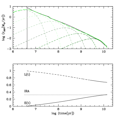
Figure 1: Top panel: the exact, normalized $r_{\rm SSP}$ for a SSP of solar metallicity as given by eq. (2), is represented by the solid line. The long-dashed line is the analytic fit obtained from eq. (11) with $k=6$, while the six components are represented by the short-dashed lines. The fit parameters are given in Table 1. Bottom panel: the exact cumulative mass fraction $E(t)$ (solid line, eq. 17), and the the locked-up fraction $L(t)=1-E(t)$. For reference, $E$ calculated in the IRA is represented by the dotted line.

As well known (e.g., Ciotti et al. 1991, Pellegrini 2012), for a SSP assembled at $t=0$, the normalized mass return rate $r_{\rm SSP}$ can be written as

$$r_{\rm SSP}(t)=\phi[M_{\rm TO}(t)]\times M_{\rm ej}[M_{\rm TO}(t)]\times|\dot{M}_{\rm TO}(t)|,$$ (2)

where $M_{\rm TO}(t)$ is the mass of the stars entering the Turn-Off phase at time $t$, and $M_{\rm ej}(M)$ is the total mass ejected by a star of initial mass $M$ in the post main sequence evolutionary phases. By construction, the mass return rate of the considered SSP is given by $R_{\rm SSP}=M_{*}\times r_{\rm SSP}$.

For a SFH characterized by a star formation rate $\psi(t)$, and a time and metallicity independent IMF, the mass return rate at the time $t$ is given by

$$R(t)=\int_{0}^{t}\psi(\tau)\,r_{\rm SSP}(t-\tau)\,d\tau.$$ (3)

Note that the lower limit of integration is arbitrary, being related to the beginning of star formation: for example, in this case we assume without loss of generality that $\psi$=0 for $t<0$. On the contrary, the upper limit of integration is physically required by the obvious fact that mass return from a stellar population cannot take place before its formation.

As pointed out in the Introduction, the integral above, when evaluated by direct sum, scales quadratically with the number of time-steps adopted to discretize the time $t$, so its computation can be extremely time-consuming. We will now show how to evaluate eq. (3) as a linear function of the number of time-steps, and without the need of storing the whole evolution of $\psi(t)$. We will refer to the rate as obtained by integrating eq. (3) with standard methods as the exact rate, while the alternative scheme here presented will be called the new method.

In the formalism of eq. (3), the mass return rate in the IRA is written as

$$R_{\rm IRA}(t)=\psi(t)\int_{0}^{\infty}r_{\rm SSP}(\tau)d\tau:$$ (4)

in practice, the IRA mass return rate is just given by the instantaneous star formation rate times the total mass fraction released by the SSP. Of course, the IRA overcomes all the problems of computational times and memory storage posed by the standard evaluation of eq. (3), but it can be properly used only when all the timescales of the problem under consideration are much longer than the lifetimes of the typical stars producing the bulk of the mass return in the SSP.

2.1 The new method

The idea behind the new method is to substitute the exact kernel $r_{\rm SSP}$ in eq. (3) with a sum of functions with special mathematical properties. We begin by illustrating the method for the case of a sum of pure exponentials. Suppose that for a given SSP formed at $t=0$ the associated $r_{\rm SSP}(t)$ can be represented with high accuracy as

$$r_{\rm SSP}(t)=\sum_{i=1}^{k}\alpha_{i}e^{-\beta_{i}t},$$ (5)

where the parameters $\alpha_{i}$ and $\beta_{i}$ are obtained by fitting the exact function given in eq. (2); note that $\alpha_{i}$ and $\beta_{i}$ are in units of inverse of time (e.g., Gyr^-1).

It follows that eq. (3) can be written as

$$R(t)=\sum_{i=1}^{k}\alpha_{i}\,I^{(0)}_{i}(t),$$ (6)

where

$$I^{(0)}_{i}(t)=\int_{0}^{t}\psi(\tau)e^{-\beta_{i}(t-\tau)}\,d\tau.$$ (7)

The meaning of the superscript “(0)” will become clear in the following. For simplicity we drop the subscript index $i$, as we now derive the generic expression for the family $I^{(0)}$, and the restoration of subscript $i$ in the resulting formulae is immediate.

It is straightforward to show that for a generic time interval $\Delta t$ (not necessarily small), the function $I^{(0)}$ can be written rigorously as

$$I^{(0)}(t+\Delta t)=e^{-\beta\Delta t}I^{(0)}(t)+J^{(0)}(t,\Delta t),$$ (8)

where

$$J^{(0)}(t,\Delta t)\equiv\int_{t}^{t+\Delta t}\psi(\tau)\,e^{-\beta(t+\Delta t-\tau)}\,d\tau.$$ (9)

In practice, at time $t+\Delta t$, each term of the sum in eq. (6) can be calculated iteratively from the values at time $t$, plus a contribution $J^{(0)}$ due to the star formation over the last time interval only. For example, if we adopt a standard trapezoidal rule,

$$J^{(0)}(t,\Delta t)\simeq{\Delta t\over 2}\left[\psi(t+\Delta t)+\psi(t)e^{-\beta\Delta t}\right],$$ (10)

and the final recursive formula for $R(t+\Delta t)$ is obtained by summation of the $k$ components by using eq. (8).

Remarkably, for reasons that will be explained below, the method can be extended by using in eq. (5) “base” functions more general than pure exponentials, namely $t^{n}e^{-\beta t}$, where $n$ is an integer (and, as discussed in the Appendix, not necessarily the same in all the $k$ components). In principle, this property allows to reproduce quite complicated time dependencies of $r_{\rm SSP}(t)$, in particular the initial rise due to the short but finite lifetimes of the most massive stars in the IMF. For example, in the illustrative case presented in Sect. 3 we found it optimal to use $n=1$ in all the components. Accordingly, we now consider

$$r_{\rm SSP}(t)=\sum_{i=1}^{k}\alpha_{i}\,t\,e^{-\beta_{i}t},$$ (11)

(where of course $\alpha_{i}$ and $\beta_{i}$ are different from those appearing in eq. (5), and the $\alpha_{i}$ are now in units of Gyr^-2). It follows that

$$R(t)=\sum_{i=1}^{k}\alpha_{i}\,I^{(1)}(t),$$ (12)

with

$$I^{(1)}(t)=\int_{0}^{t}\psi(\tau)\,(t-\tau)e^{-\beta(t-\tau)}\,d\tau.$$ (13)

Simple algebra shows that for a generic time interval $\Delta t$,

$$I^{(1)}(t+\Delta t)=e^{-\beta\Delta t}\left[I^{(1)}(t)+I^{(0)}(t)\Delta t\right]+J^{(1)}(t,\Delta t),$$ (14)

where $I^{(0)}(t)$ is still given by eqs. (7)-(8) with the new $\alpha_{i}$ and $\beta_{i}$, and

$$J^{(1)}(t,\Delta t)\equiv\int_{t}^{t+\Delta t}\psi(\tau)\,(t+\Delta t-\tau)e^{-\beta(t+\Delta t-\tau)}\,d\tau.$$ (15)

The integral $J^{(1)}$ over the last time-step can be evaluated with a simple trapezoidal rule, obtaining in this case

$$J^{(1)}(t,\Delta t)\simeq{\Delta t^{2}\over 2}\psi(t)e^{-\beta\Delta t}.$$ (16)

As anticipated above, the extension of the scheme of eqs. (8) and (14) to functions $t^{n}e^{-\beta t}$ with integer $n\geq 0$ is straightforward by using the binomial theorem, and the resulting recursive formula for the functions $I^{(n)}(t+\Delta t)$ involves the evaluation and the storing of the functions $I^{(j)}(t)$ for $j=0,1,...,n$. One may ask why the method works, i.e., why it is possible for this set of functions to evaluate a convolution integral over the whole SFH just by keeping track (for each of them) of $n+1$ values relative to the previous time. The reason is easily explained following the general argument in the Appendix: here we just stress that if the kernel $r_{\rm SSP}$ obeys a linear ordinary differential equation (ODE) with constant coefficients, then also $R$ obeys a linear ODE with constant coefficients of the same degree, so that integration of eq. (3) is equivalent to the integration of the associated ODE, and the number of needed initial data is given by the order of the equation. For example, in the case of a single function $t^{n}e^{-\beta t}$ the order of the ODE is $n+1$, the number of quantities needed to be stored to evaluate $I^{(n)}$. When $r_{\rm SSP}$ is given by a sum of functions the argument is technically more complicated, but conceptually identical, and following the Appendix one can show that the specific case of eq. (11) requires the storing of $2\,k$ values at the previous time. For the more mathematically inclined readers, in the Appendix we derive the ODE for $R(t)$ in the case of the most general combination of functions $t^{n}e^{-\beta t}$ with arbitrary $n$, and we also briefly comment on the relation of the present method with the theory of Green functions.

3 Results

In the example considered here for illustrative purposes of the method, we evaluate $r_{\rm SSP}$ from eq. (2) by using $M_{\rm ej}(M)$ as given by Van den Hoeck & Groenewegen (1997) for low and intermediate mass stars ($0.8\leq M\leq 8$), and by Woosley & Weaver (1995) for massive stars ($M>8$). In particular, the adopted $M_{\rm ej}$ holds for a stellar metallicity $Z=0.02$, very close to the concordance solar value of 0.015 (e.g, Lodders 2003). For the IMF we adopt a Kroupa et al. (1993) $\phi(M)$ with $M_{\rm inf}=0.1$ and $M_{\rm sup}=40$, while the stellar lifetimes are taken from Padovani & Matteucci (1993). Of course, the general scheme of the method is independent of the specific choices made, and different prescriptions for the properties of the SSP can be considered as well (e.g., Ciotti et al. 1991, Pellegrini 2012).

3.1 Fitting the $r_{\rm SSP}$

For the SSP described above Fig. 1 (top panel, solid line) shows the exact normalized mass return rate $r_{\rm SSP}$ calculated according to eq. (2) (top panel, solid line), and the corresponding returned cumulative mass fraction as a function of cosmic time (bottom panel, solid line)

$$E(t)=\int_{0}^{t}r_{\rm SSP}(\tau)d\tau.$$ (17)

The bottom panel also includes the quantity $L(t)=1-E(t)$, i.e. the fraction of mass locked up in living stars and remnants (Portinari et al. 2004). In this example, $E(\infty)\simeq 33$% and $L(\infty)\simeq 67$%. For comparison, the dotted line represents the cumulative returned mass fraction calculated assuming the IRA, and it is apparent how this assumption leads to overestimate the mass return of a SSP, in particular at early times.

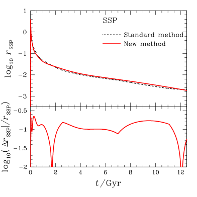
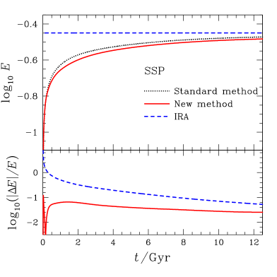
Figure 2: Left panels: exact specific mass return rate $r_{\rm SSP}$ as given by eq. (2) (dotted line), along with its fit from eq. (11) for the parameters reported in Table 1 (red solid line). The relative error between the two rates is shown in the bottom panel. Right panels: the cumulative ejected mass computed from the integral of the the exact rate (dotted) and of the fit (solid). The dashed line represents the same quantities calculated assuming the IRA. In the bottom-right panel, the relative errors with respect to the exact rate are shown, as computed by means of the new method (solid line) and in the case of the IRA.

In Fig. 1 (top panel, short dashed lines) we also show the separate contribution of the six fit components in eq. (11), whose parameters $\alpha_{i}$ and $\beta_{i}$ are reported in Tab. 1, together with their sum (long dashed line). As can be seen from Tab. 1, the best fit parameters obey

$$\sum_{i=1}^{6}\frac{\alpha_{i}}{\beta_{i}^{2}}\simeq 0.328$$ (18)

i.e. the fit in eq. (11) conserves the total mass almost perfectly. The plot in terms of the logarithm of time allows to appreciate how well the fit reproduces the exact $r_{\rm SSP}$, with the exception of the few Myrs after the SSP formation. This is due to the fact that the exact $r_{\rm SSP}$ presents a discontinuity at the time corresponding to the lifetime of the highest mass stars (4 Myr for a $40M_{\odot}$ star): in any case, the functions $te^{-\beta t}$ allow to reproduce the initial rise better than pure exponentials, and even better results would be obtained by using functions $t^{n}e^{-\beta t}$ with larger values of $n$. Here, for presentation purposes, we restrict to $n=1$ as a compromise between accuracy and algebraic simplicity.

The overall impact of the initial discontinuity on the resulting mass return rate is negligible, as can be seen from Fig. 2. In the left-hand panels we show again the exact rate $r_{\rm SSP}$ obtained by evaluation of eq. (2) (top panel, dotted line) compared to the rate obtained by summing the six fit components (red solid line), and the relative error between the fit function and the exact rate $r_{\rm SSP}$ as a function of time (bottom panel). In the right-hand panels we show the cumulative returned mass $E(t)$ and the associated relative error for the exact $r_{\rm SSP}$ (dotted line), for the new method (red solid line), and in the case of IRA (blu dashed line), respectively. Note how the relative error of the new method is significantly smaller than the one obtained with the IRA, especially at early times.

Table 1: Parameters of the six functions $\alpha_{i}\,t\,e^{-\beta_{i}t}$ used for the fit of the $r_{\rm SSP}$ considered in Section 3.1.

$\alpha_{i}$ (Gyr-2)	$\beta_{i}$ (Gyr-1)
$7.7624\times 10^{-3}$	$3.1623\times 10^{-1}$
$9.5499\times 10^{-2}$	$1.2589\leavevmode\nobreak\ \leavevmode\nobreak\ \leavevmode\nobreak\ \leavevmode\nobreak\ \leavevmode\nobreak\ \leavevmode\nobreak\ \leavevmode\nobreak\ \leavevmode\nobreak\ \leavevmode\nobreak\ \leavevmode\nobreak\ \leavevmode\nobreak\ \leavevmode\nobreak\ \leavevmode\nobreak\$
$1.3183\leavevmode\nobreak\ \leavevmode\nobreak\ \leavevmode\nobreak\ \leavevmode\nobreak\ \leavevmode\nobreak\ \leavevmode\nobreak\ \leavevmode\nobreak\ \leavevmode\nobreak\ \leavevmode\nobreak\ \leavevmode\nobreak\ \leavevmode\nobreak\ \leavevmode\nobreak\ \leavevmode\nobreak\$	$5.0119\leavevmode\nobreak\ \leavevmode\nobreak\ \leavevmode\nobreak\ \leavevmode\nobreak\ \leavevmode\nobreak\ \leavevmode\nobreak\ \leavevmode\nobreak\ \leavevmode\nobreak\ \leavevmode\nobreak\ \leavevmode\nobreak\ \leavevmode\nobreak\ \leavevmode\nobreak\ \leavevmode\nobreak\$
$21.380\leavevmode\nobreak\ \leavevmode\nobreak\ \leavevmode\nobreak\ \leavevmode\nobreak\ \leavevmode\nobreak\ \leavevmode\nobreak\ \leavevmode\nobreak\ \leavevmode\nobreak\ \leavevmode\nobreak\ \leavevmode\nobreak\ \leavevmode\nobreak\ \leavevmode\nobreak\ \leavevmode\nobreak\$	$19.953\leavevmode\nobreak\ \leavevmode\nobreak\ \leavevmode\nobreak\ \leavevmode\nobreak\ \leavevmode\nobreak\ \leavevmode\nobreak\ \leavevmode\nobreak\ \leavevmode\nobreak\ \leavevmode\nobreak\ \leavevmode\nobreak\ \leavevmode\nobreak\ \leavevmode\nobreak\ \leavevmode\nobreak\$
$2.9512\times 10^{2}$	$79.433\leavevmode\nobreak\ \leavevmode\nobreak\ \leavevmode\nobreak\ \leavevmode\nobreak\ \leavevmode\nobreak\ \leavevmode\nobreak\ \leavevmode\nobreak\ \leavevmode\nobreak\ \leavevmode\nobreak\ \leavevmode\nobreak\ \leavevmode\nobreak\ \leavevmode\nobreak\ \leavevmode\nobreak\$
$3.7153\times 10^{3}$	$3.1623\times 10^{2}$

3.2 Multiple stellar population

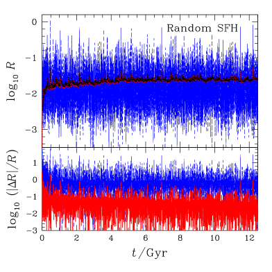
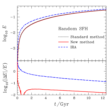
Figure 3: Left panels: time evolution of the mass return rate $R$ of a multiple stellar population originated by a SFH consisting of several bursts of random amplitude, as described in Sect. 3.2. The black solid line is the rate computed with the standard method, the red line with the new method, and the blue line by using the IRA. This latter line also visualizes the adopted SFH, because from eq. (4) $R_{\rm IRA}(t)\propto\psi(t)$. The relative error of the mass return rate is shown in the bottom panel for the new method (red) and assuming the IRA (blue). Right panels: the cumulative mass return $E$ and the relative errors are shown, with the same line styles as in the left panels. The quantities $R$ and $E$ are normalized to the total stellar mass formed over the simulation, and the time-step is $\Delta t=1.4$ Myr.

We now move to consider the case of the mass return rate of a multiple stellar population originated by a complex SFH.

In order to test the performance (in terms of computational speed and accuracy) of the new method, we consider an artificial case, characterized by a large number of star-formation bursts of random amplitude. This case is relevant since it mimics the SFHs commonly encountered in SAMs, and which are typical of systems undergoing a large number of mergers and interactions, such as the ones resulting from the intricate merging trees of giant galaxies (Somerville & Kolatt 1999; Lanzoni et al. 2000; Calura & Menci 2009; Yates et al. 2013), or star formation induced by AGN activity in the inner regions of the host systems (Ciotti & Ostriker 2007). In practice, we adopt a SFH $\psi(t)$ in which, at each time-step, $\log_{10}\psi$ is extracted randomly from a normal distribution with standard deviation $0.5$. In the following experiment, the time-step is kept constant, $\Delta t=1.4$ Myr, suited to resolve the time contribution to the mass return rate of the most massive stars at early times (in hydrodynamical simulations considerably shorter time-steps are common, down to $10^{3}-10^{4}$ yr or less).

The behaviour of $\psi(t)$ is visualized by the blue dashed line in Fig. 3 (top-left panel), representing the mass return rate in the IRA (which is proportional to $\psi$, see eq. 4). The resulting mass return rate is also shown for the the standard method (black solid line) and with the new method (red line): the relative errors with respect to the exact values of the mass return rate are shown in the bottom-left panel. The most striking feature is the large scatter in $R_{\rm IRA}$ (more than two orders of magnitude) compared to the exact rate, which instead is almost perfectly matched by the rate obtained with the new method. The relative errors represented in the bottom-left panel quantify the performance of IRA and of the new method: in general, the peaks in the relative errors of the IRA are related with peaks in the instantaneous SFH $\psi(t)$. Such peaks are also present in the mass return computed with the new method, as a consequence of the initial discontinuity following each burst, as described above. However, the amplitude of these error is significantly smaller than in the IRA case, as apparent.

The cumulative mass return for the multi-burst SFH is shown in the right panels of Fig. 3, where the quantity $E(t)$ is normalized to the stellar mass formed over the entire simulation. The top-right panel shows this quantity for the exact case, for the IRA case, and for the new method, while the bottom-right panel shows the relative error between the IRA and the exact case, and between the new method and the exact case. Note the remarkable accuracy of the new method in the multiple population case, actually even better than in the case of a SSP. This is not surprising, as for a multiple stellar population the IRA is, in practice, always in the most critical regime (just after a burst), and its error is of a magnitude similar to that presented at early times in Fig. 2 (bottom right panel).

3.3 Computational advantages of the new method

As already discussed, the IRA presents considerable advantages in terms of computational time and does not require any storage regarding ages and metallicities of composite stellar populations. Essentially, at any time, the mass return rate is calculated directly from the physical properties of the system at that particular time, i.e. directly from the instantaneous value of the star formation rate (see eq. 4). The major problem with the IRA is that it breaks down at short times after a starburst event, when the very short characteristic heating and cooling times would lead to large overestimates of the mass return rate, that in turn can seriously affect the numerical computations by altering the available mass budget.

The method presented in this paper offers the possibility to compute the mass return rate for arbitrarily complicated SFHs, at a computational cost considerably lower than that required when the exact method is used, yet maintaining the full accuracy. The computational gain of the new method with respect to the standard method can be estimated by considering the number of needed operations. The computational time of the exact calculation scales with the total number of time-steps $N_{\rm step}$ as $T_{\rm CPU,standard}\propto N_{\rm step}(N_{\rm step}+1)/2$, since $j$ operations are needed to compute the mass return rate at the $j$-th time-step. With the new method, $T_{\rm CPU,new}\propto(n+1)kN_{\rm step}$, because at each time the $n+1$ integrals over the last time step $J^{(0)},\ldots,J^{(n)}$ must be computed for each of the $k$ functions used in the fit. Therefore, $T_{\rm CPU,new}/T_{\rm CPU,standard}\sim 2(n+1)k/N_{\rm step}$: when the other parameters are fixed, the computational gain of the new method over the standard method increases linearly with $N_{\rm step}$, i.e. it increases for decreasing $\Delta t$ (at fixed total time span). Note that the CPU time of the new method scales with $N_{\rm step}$ as in the IRA.

The actual computational gain of the new method obtained in numerical experiments similar to that described in Sect. 3.2, where different $\Delta t$ are adopted, is shown in Fig. 4, plotting the CPU time (in arbitrary units) required to evaluate the mass return for the exact method (dotted line), the new method (red line), and the IRA (dashed line), as a function of the total number of time-steps $N_{\rm step}$. For our reference case with $\Delta t=1.4$ Myr, we have $N_{\rm step}=8929$, $k=6$, $n=1$, so we expect $T_{\rm CPU,new}/T_{\rm CPU,standard}\simeq 2.7\times 10^{-3}$. In fact, the experiment shows that the CPU time for the new method is a factor $\approx 500$ shorter than for the standard method, in agreement with the analytic estimate. From Fig. 4 it is also apparent that the actual scaling with $N_{\rm step}$ nicely follows the expected scaling ($T_{\rm CPU,new}\propto T_{\rm CPU,IRA}\propto N_{\rm step}$, $T_{\rm CPU,standard}\propto N_{\rm step}^{2}$). We remark again that in hydrodynamical simulations the actual $\Delta t$ can easily be one or two orders of magnitude shorter than 1 Myr, so that the gain of the new method will increase accordingly; moreover, this further gain will also be multiplied by the number of grid points.

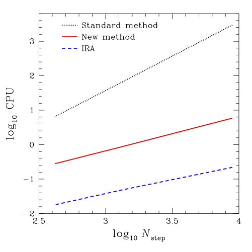
Figure 4: CPU time (in arbitrary units) required by the computation of the mass return rate by means of the standard method (dotted line), the new method (solid line) and the IRA (dashed line), as a function of the total number of time-steps $N_{\rm step}$. The case discussed in Sect. 3.2 corresponds to $\log_{10}N_{\rm step}\simeq 3.95$.

4 Conclusions

The mass returned to the ambient medium by evolving stellar populations represents a significant fraction of their initial mass (20% to 30% for realistic IMFs), and thus being a non negligible contribution to the evolution of stellar systems. For example, in elliptical galaxies the total mass of the returned gas is almost two orders of magnitude larger than the observed masses of central SMBHs, requiring important AGN feedback effects to prevent accretion in absence of other mechanisms able to eject the metal rich gas from the galaxies (e.g., Ciotti & Ostriker 2001).

In numerical problems dealing with the evolution of stellar populations and their mass return, when the characteristic times are longer than the stellar evolutionary times, the IRA is a useful approximation of the convolution integral describing mass return, allowing for fast and accurate computations. However, in hydrodynamical studies of star formation, of the interplay between central starbursts and AGN feedback in the coevolution of galaxies and their central SMBHs, and of the origin of multiple stellar populations in globular clusters, the dominance of short characteristic times ($\simeq 10^{3}$ yr of even less), coupled with thousands (or more) spatial grid points, requires the detailed evaluation of the convolution integral. This makes the simulations excessively demanding in terms of computer memory and computational time, due to the need of storing the whole SFH at each grid point and to the number of evaluations to be performed increasing quadratically with the number of time steps.

In order to overcome these problems we developed a fast and accurate method to evaluate the mass return rate from stellar populations with arbitrarily complicated SFHs. The method presents great computational advantages over the direct evaluation of the convolution integral (the computation time scales linearly with the number of time steps), yet its accuracy is much better than that achievable with the IRA, especially in the case of multiple populations, when the clock of the mass return rate is reset at each star formation event. The new method can be easily implemented in semi-analytical models and in grid-based hydrodynamical simulations, and it requires to fit the mass return rate from the adopted SSP by means of simple functions, solutions of linear ODEs with constant coefficients. We have shown how these functions allow to evaluate, at any time-step, the mass return rate directly from its value at the previous time step, plus a contribution depending only on the star formation over the last time step. The general mathematical framework is presented in the Appendix. In this paper, as a specific application, we have shown that the use of a linear combination of the functions $t\,e^{-\beta t}$ is enough to achieve very accurate results: with arbitrarily complicated SFHs, the computed mass return rate from the resulting multiple stellar population deviates by amounts of a few percent from the exact value, and this avoiding the storage of the SFH itself.

We conclude by noticing that the presented method, applying in general to the treatment of time convolution integrals, can be also used in problems different from that discussed in this paper, for example to study the return of single chemical elements from multiple stellar populations (as in starbursts), or to describe the time evolution of the SNIa rate in star forming events.

Appendix A The general ODE for the mass return rate

For ease of notation we rewrite eq. (3) as

$$Y(t)=\int_{-\infty}^{t}\psi(\tau)y(t-\tau)\,d\tau,$$ (19)

where the meaning of $Y$ and $y$ is obvious, and the lower limit of integration allows full generality in the treatment. Let assume that $y$ is a solution of a homogeneous, constant-coefficients linear ODE of order $n$, i.e.,

$$\sum_{i=0}^{n}c_{i}y^{(i)}=0,$$ (20)

where $c_{i}$ are constants, $y^{(i)}\equiv d^{i}y/dt^{i}$, and $y^{(0)}\equiv y$. Taking for granted that all the technical requirements of convergence and regularity are satisfied, mathematical induction proves that the time derivatives of the function $Y$ can be written as

$$Y^{(i)}(t)=\sum_{j=0}^{i-1}\psi^{(i-j-1)}(t)y^{(j)}(0)+\int_{-\infty}^{t}\psi(\tau)y^{(i)}(t-\tau)\,d\tau,$$ (21)

for $i=1,2,...,n$. After multiplication of eq. (A3) by $c_{i}$ and summation over $i$, from eq. (A2) it follows that $Y$ also obeys the generally non-homogeneous constant-coefficients linear ODE of order $n$

$$\sum_{i=0}^{n}c_{i}Y^{(i)}=\sum_{i=0}^{n}\sum_{j=0}^{i-1}c_{i}\psi^{(i-j-1)}(t)y^{(j)}(0).$$ (22)

Note that the assumption of constant coefficients is important here, because the vanishing of the resulting linear combination of integrals at the r.h.s. of eq. (A3) rests on two facts: 1) the $c_{i}$ can be carried under sign of integration (this would be true also for time-dependent coefficients $c_{i}$), and 2) if $y(t)$ is a solution of eq. (A2), then also $y(t-\tau)$ is a solution (this in general would not be true for time-dependent $c_{i}$). Therefore, if the kernel $r_{\rm SSP}$ is solution of a constant-coefficients linear ODE of order $n$, also the mass return rate $R$ can be represented as a solution of constant-coefficients linear ODE of order $n$, and so $n$ integration constants are required for its complete determination.

Suppose now to consider the following generalization of eqs. (5) and (11)

$$y(t)=\sum_{i=1}^{k}\sum_{j=0}^{n_{i}}\alpha_{ij}t^{j}e^{-\beta_{i}t},$$ (23)

where $\alpha_{ij}=0$ for $j>n_{i}$, $\alpha_{ij}\neq 0$ for $j=n_{i}$, and for $j<n_{i}$ the coefficients $\alpha_{ij}$ may be zero or not; without loss of generality we assume that all the $\beta_{i}$ are different. Note that in eq. (A5) we consider the possibility that more than one power term $t^{j}$ is associated with a given $\beta_{i}$, and that the maximum values $n_{i}$ differ for different $\beta_{i}$. In this formalism eq. (5) is obtained for $n_{i}=0$ and $\alpha_{i0}=\alpha_{i}$ ($i=1,...,k$), while eq. (11) for $n_{i}=1$, $\alpha_{i0}=0$, and $\alpha_{i1}=\alpha_{i}$ ($i=1,...,k$).

We now construct the ODE for $y$ in eq. (A5), so that also the ODE for the mass return rate $R(t)$ can be explicitly obtained in this general case accordingly to eq. (A4). From the theory of ODEs (e.g., Ince 1956) it is known that the function $t^{n}e^{-\beta t}$ is solution of a constant-coefficients linear ODE, where the root $-\beta$ of the associated characteristic polynomial has (at least) algebraic multiplicity $n+1$. Therefore, the minimum characteristic polynomial of the ODE admitting eq. (A5) as solution is

$$\prod\limits_{i=1}^{k}(\lambda+\beta_{i})^{n_{i}+1}=0,$$ (24)

and the corresponding ODE of order $\sum_{i=1}^{k}(n_{i}+1)$ is obtained by the substitution $\lambda=d/dt$.

A final comment is in order. Due to the formal similarity of eq. (A1) with the convolution integral appearing in the theory of Green functions, one may ask whether $y(t)\theta(t)$ (where $\theta$ is the Heaviside step function) is the Green function, vanishing for $t<0$, of the ODE (A2). The answer is negative, as $y(t)$ in general lacks the needed regularity at $t=0$ (e.g., Bender & Orszag 1978). In fact, from the request of vanishing for $t<0$, it follows that the function $y(t)\theta(t)$ is a genuine Green function if and only if the time derivative of order $\sum_{i=1}^{k}(n_{i}+1)-1$ of $y(t)$ evaluated at $t=0$ presents a finite jump, while all the remaining derivatives of $y(t)$ up to the order $\sum_{i=1}^{k}(n_{i}+1)-2$ evaluated at $t=0$ vanish. These requests impose constraints on the values $\alpha_{ij}$. However, in our method the $\alpha_{ij}$ are given as best-fit parameters of the kernel function (in practice, by the request of reproducing $r_{\rm SSP}$), so that $y(t)$ in general does not satisfy the regularity conditions at $t=0$. However, it is easy to show that in the case of a single-component fit ($k=1$), the function $t^{n}e^{-\beta t}\theta(t)$ with $n\geq 0$ is the Green function for the corresponding linear ODE of order $n+1$.

References

- [] Baugh C. M., 2006, Rep. Prog. Phys., 69, 3101
- [] Bender, C.M., & Orszag, S.A., 1978, “Advanced mathematical methods for scientists and engineers”, McGraw-Hill (New York)
- [] Calura F., Menci N., 2009, MNRAS, 400, 1347
- [] Chabrier, G., 2003, PASP, 115, 763
- [] Ciotti, L., D’Ercole, A., Pellegrini, S., Renzini, A., 1991, ApJ, 376, 380
- [] Ciotti, L., & Ostriker, J.P., 1997, ApJL, 487, 105
- [] Ciotti L., Ostriker J.P., 2001, ApJ, 551, 131
- [] Ciotti, L., Ostriker, J.P., 2007, ApJ, 665, 1038
- [] Ciotti, L., & Ostriker, J.P., 2012, in “Hot Interstellar Matter in Elliptical Galaxies”, D.W. Kim and S. Pellegrini Eds., Astrophys. and Space Sci. Library, vol. 378, p.83 (Springer)
- [] D’Ercole, A., D’Antona, F., Carini, R., Vesperini, E., & Ventura P., 2012, MNRAS, 423, 1521
- [] Greggio, L., 2005, A&A, 441, 1055
- [] Ince, E.L., 1956 “Ordinary differential equations”, Dover
- [] Ishibashi, W., & Fabian, A.C., 2012, MNRAS, 427, 2998
- [] Kroupa P., Tout C. A., Gilmore G., 1993, MNRAS, 262, 545
- [] Krumholz, M. R. 2011, in AIP Conf. Ser., 1386, eds. E. Telles, R. Dupke, & D. Lazzaro, 9
- [] Lanzoni B., Mamon G. A., Guiderdoni B., 2000, MNRAS, 312, 781
- [] Lodders K. 2003, ApJ, 591, 1220
- [] Lusso E., Ciotti L., 2011, A&A, 525, 115
- [] Maraston C., 1998, MNRAS, 300, 872
- [] Mathews, W.G., & Brighenti, F., 2003, ARAA, 41, 191
- [] Matteucci F., 2001, Astrophys. Space Sci. Library Vol. 253, The Chemical Evolution of the Galaxy. Kluwer, Dordrecht, p. 293
- [] Matteucci F., & Greggio L., 1986, A&A, 154, 279
- [] Norman, C., & Scoville, 1988, ApJ, 332, 163
- [] Padovani P., & Matteucci F., 1993, ApJ, 416, 26
- [] Pellegrini S, 2012, in “Hot Interstellar Matter in Elliptical Galaxies”, D.W. Kim and S. Pellegrini Eds., Astrophys. and Space Sci. Library, vol. 378, p.21 (Springer)
- [] Piotto, G. et al., 2007, ApJL, 661, 53
- [] Portinari L., Moretti A., Chiosi C., Sommer-Larsen J., 2004, ApJ, 604, 579
- [] Renzini, A., 2008, MNRAS, 391, 354
- [] Scalo J. M., 1986, Fundam. Cosmic Phys., 11, 1
- [] Shcherbakov, R.V., Wong, K.-W., Irwin, J.A., & Reynolds, C.S., preprint (arXiv1308.4133)
- [] Somerville R. S., Kolatt T. S., 1999MNRAS.305, .1S
- [] Starkenburg E., Helmi, A., De Lucia, G., Li, Y.-S., Navarro, J. F., Font, A. S., Frenk, C. S., Springel, V., Vera-Ciro, C. A., White, S. D. M., 2013, MNRAS, 429, 725
- [] Tabor G, & Binney, J., 1993, MNRAS, 263, 323
- [] Tinsley B. M., 1980, Fund. Cosmic Phys., 5, 287
- [] Tosi M. 1988, A&A, 197, 33
- [] Van den Hoeck L. B., Groenwegen M. A. T., 1997, A&AS, 123, 305
- [] Woosley S. E., Weaver T. A. 1995, ApJS, 101, 181
- [] Yates R. M., Henriques B., Thomas P. A., Kauffmann G., Johansson J., White S. D. M., 2013, MNRAS, 435, 3500
- [] Zubovas, K., Nayakshin, S., King, A., & Wilkinson, M., 2013, MNRAS, 433, 3079