Long-term Variability in the Length of the Solar Cycle

Abstract

The recent paucity of sunspots and the delay in the expected start of Solar Cycle 24 have drawn attention to the challenges involved in predicting solar activity. Traditional models of the solar cycle usually require information about the starting time and rise time as well as the shape and amplitude of the cycle. With this tutorial, we investigate the variations in the length of the sunspot number cycle and examine whether the variability can be explained in terms of a secular pattern. We identified long-term cycles in archival data from 1610 – 2000 using median trace analyses of the cycle length and power spectrum analyses of the (O-C) residuals of the dates of sunspot minima and maxima. Median trace analyses of data spanning 385 years indicate a cycle length with a period of 183 - 243 years, and a power spectrum analysis identifies a period of 188 $\pm$ 38 years. We also find a correspondence between the times of historic minima and the length of the sunspot cycle, such that the cycle length increases during the time when the number of spots is at a minimum. In particular, the cycle length was growing during the Maunder Minimum when almost no sunspots were visible on the Sun. Our study suggests that the length of the sunspot number cycle should increase gradually, on average, over the next $\sim$75 years, accompanied by a gradual decrease in the number of sunspots. This information should be considered in cycle prediction models to provide better estimates of the starting time of each cycle.

1. Introduction

Solar Cycle 24 was predicted to begin in 2008 March ($\pm$ 6 months), and peak in late 2011 or mid-2012, with a cycle length of 11.75 years. So, the recent paucity of sunspots and the delay in the expected start of Solar Cycle 24 were unexpected, even though it is well known that solar cycles are challenging to forecast (Biesecker, 2007; Kilcik et al., 2009). Since traditional models based on sunspot data require information about the starting and rise times, and also the shape and amplitude of the cycle, the fine details of a given solar cycle can be predicted accurately only after a cycle has begun (e.g., Elling & Schwentek 1992; Joselyn et al. 1996). Many of these models analyze a large number of previous cycles in order to predict the pattern for the new cycle. In contrast, the technique of helioseismology does not depend on sunspot data and has been used to predict activity two cycles into the future; this method was used by Dikpati, de Toma & Gilman (2006) to predict that sunspots will cover a larger area of the sun during Cycle 24 than in previous cycles, and that the cycle will reach its peak about 2012, one year later than forecast by alternative methods based on sunspot data (e.g., de Toma et al. 2004).

The measurements of the length of the sunspot cycle show that the cycle varies typically between 10 and 12 years. Moreover, these variations in the cycle length have been associated with changes in the global climate (Wilson, 2006; Wilson et al., 2008). In addition, the Maunder Minimum illustrates a connection between a paucity of sunspots and cooler than average temperatures on Earth.

The length of the sunspot cycle was first measured by Heinrich Schwabe in 1843 when he identified a 10-year periodicity in the pattern of sunspots from a 17-year study conducted between 1826 and 1843 (Schwabe, 1844). In 1848, Rudolph Wolf introduced the relative sunspot number, R, organized a program of daily observations of sunspots, and reanalyzed all earlier data to find that the average length of a solar cycle was about 11 yrs. For more than two centuries, solar physicists applied a variety of techniques to determine the nature of the solar cycle. The earliest methods involved counting sunspot numbers and determining durations of cyclic activity from sunspot minimum to minimum using the “smoothed monthly mean sunspot number” (Waldmeier, 1961; Wilson, 1987, 1994). The “Group sunspot number” introduced by Hoyt & Schatten (1998) is another well-documented data set and provides comparable results to those derived from relative sunspot numbers. In addition, sunspot area measurements since 1874 describe the total surface area of the solar disk covered by sunspots at a given time.

The analysis of sunspot numbers or sunspot areas is often referred to as a one-dimensional approach because there is only one independent variable, namely sunspot numbers or areas (Wilson, 1994). Recently, Li et al. (2005) introduced a new parameter called the “sunspot unit area” in an effort to combine the information about the sunspot numbers and sunspot areas to derive the length of the cycle. There is also a two-dimensional approach in which the latitude of an observed sunspot is introduced as a second independent variable (Wilson, 1994). When sunspots first appear on the solar surface they tend to originate at latitudes around 40 degrees and migrate toward the solar equator. When such migrant activity is taken into account it can be shown that there is an overlap between successive cycles, since a new cycle begins while its predecessor is still decaying. This overlap became obvious when Maunder (1904) published his butterfly diagram and demonstrated the latitude drift of sunspots throughout the cycles. Maunder’s butterfly diagram showed that although the length of time between sunspot minima is on average 11 years, successive cycles actually overlap by $\sim$ 1 to 2 years. In addition, Wilson (1987) found that there were distinct solar cycles lasting 10 years as well as cycles lasting 12 years. This type of behavior suggests that there could be a periodic pattern in the length of the sunspot cycle. A summary of analyses of the sunspot cycle is found in Kuklin (1976) and a more recent review of the long-term variability is given by Usoskin & Mursula (2003).

Sunspot number data collected prior to the 1700’s show epochs in which almost no sunspots were visible on the solar surface. One such epoch, known as the Maunder Minimum, occurred between the years 1642 and 1705, during which the number of sunspots recorded was very low in comparison to later epochs (Wilson, 1994). Geophysical data and tree-ring radiocarbon data, which contain residual traces of solar activity (Baliunas & Vaughan, 1985), were used to examine whether the Maunder period truly had a lower number of sunspots or whether it was simply a period in which little data had been collected or large degrees of errors existed. These studies showed that the timing of the Maunder Minimum was fairly accurate because of the high quality of sunspot data during that period, including sunspot drawings, and the dates are strongly correlated with geophysical data. Other epochs of significantly reduced solar activity include the Oort Minimum from 1010 - 1050, the Wolf Minimum from 1280 - 1340, the Spörer Minimum from 1420 - 1530 (Eddy, 1977; Stuiver & Quay, 1980; Siscoe, 1980), and the Dalton Minimum from 1790 - 1820 (Usoskin & Mursula, 2003). These minima have been derived from historical sunspot records, auroral histories (Eddy, 1976), and physical models which link the solar cycle to dendrochronologically-dated radiocarbon concentrations (Solanki et al., 2004).

Our interest in predicting flaring activity cycles on cool stars (e.g., Richards, Waltman, Ghigo, & Richards 2003) led us to investigate the long-term behavior of the solar cycle since solar flares display a typical average 11-year cycle like sunspots (Balasubramaniam & Regan, 1994). In this paper, the preliminary results of which were published in Rogers & Richards (2004) and Rogers, Richards, & Richards (2006), we investigate the variations in the length of the sunspot number cycle and examine whether the variability can be explained in terms of a secular pattern. Our analysis can serve as a tutorial. We apply classical one-dimensional techniques to recalculate the periodicities of solar activity using the sunspot number and area data to provide internal consistency in our analysis of the long-term behavior. These results are then used as a basis in the subsequent study of the sun’s long-term behavior. In §2 we discuss the source of the data; in §3 we describe the derivation of the cycle from sunspot numbers and sunspot areas using two independent techniques; in §4 we examine the variability in the cycle length based on the times of cycle minima and maxima using two independent techniques; and in §5 we discuss the results.

Table 1Duration of the Data

Data Set		Duration of Data
Spot Number	Daily	1818 Jan 8 - 2005 Jan 31
	Monthly	1749 Jan - 2005 Jan
	Yearly	1700 - 2004
Spot Area	Daily	1874 May 9 - 2005 Feb 28
	Monthly	1874 May - 2005 Feb
	Yearly	1874 - 2004

2. Data Collection

The sunspot data used in this work were collected from archival sources that catalog sunspot numbers and sunspot areas, as well as the measured length of the sunspot cycle. The sunspot number data, covering the years from 1700 - 2005, were archived by the National Geophysical Data Center (NGDC). These data are listed in individual sets of daily, monthly, and yearly numbers. The relative sunspot number, R, is defined as R = K (10g + s), where g is the number of sunspot groups, s is the total number of distinct spots, and the scale factor K (usually less than unity) depends on the observer and is “intended to effect the conversion to the scale originated by Wolf” (Coffey & Erwin, 2004). The scale factor was 1 for the original Wolf sunspot number calculation. The spot number data sets are tabulated in Table 1 and plotted in Figure 1.

Table 2Length of the Sunspot Cycle

		Cycle Length	Cycle Length
Year of	Year of	(from minima)	(from maxima)
Minimum	Maximum	(yr)	(yr)
1610.8	1615.5	8.2	10.5
1619.0	1626.0	15.0	13.5
1634.0	1639.5	11.0	9.5
1645.0	1649.0	10.0	11.0
1655.0	1660.0	11.0	15.0
1666.0	1675.0	13.5	10.0
1679.5	1685.0	10.0	8.0
1689.0	1693.0	8.5	12.5
1698.0	1705.5	14.0	12.7
1712.0	1718.2	11.5	9.3
1723.5	1727.5	10.5	11.2
1734.0	1738.7	11.0	11.6
1745.0	1750.3	10.2	11.2
1755.2	1761.5	11.3	8.2
1766.5	1769.7	9.0	8.7
1775.5	1778.4	9.2	9.7
1784.7	1788.1	13.6	17.1
1798.3	1805.2	12.3	11.2
1810.6	1816.4	12.7	13.5
1823.3	1829.9	10.6	7.3
1833.9	1837.2	9.6	10.9
1843.5	1848.1	12.5	12.0
1856.0	1860.1	11.2	10.5
1867.2	1870.6	11.7	13.3
1878.9	1883.9	10.7	10.2
1889.6	1894.1	12.1	12.9
1901.7	1907.0	11.9	10.6
1913.6	1917.6	10.0	10.8
1923.6	1928.4	10.2	9.0
1933.8	1937.4	10.4	10.1
1944.2	1947.5	10.1	10.4
1954.3	1957.9	10.6	11.0
1964.9	1968.9	11.6	11.0
1976.5	1979.9	10.3	9.7
1986.8	1989.6	9.7	10.7
1996.5	2000.3	–	–
Average		11.0$\pm$1.5	11.0$\pm$2.0

The sunspot area data, beginning on 1874 May 9, were compiled by the Royal Greenwich Observatory from a small network of observatories. In 1976, the United States Air Force began compiling its own database from its Solar Optical Observing Network (SOON) and the work continued with the help of the National Oceanic and Atmospheric Administration (NOAA) (Hathaway, 2004). The NASA compilation of these separate data sets lists sunspot area as the total whole spot area in millionths of solar hemispheres. We have analyzed the compiled daily sunspot areas as well as their monthly and yearly sums. The sunspot area data sets were tabulated in Table 1 and plotted in Figure 2. There may be subtle differences between the two data sets since the sunspot number and area data were collected in different ways and by different groups, but these differences should reveal themselves when the data are analyzed.

The sunspot number cycle data from years 1610 to 2000 are shown in Table 2. This table displays the dates of cycle minima and maxima as well as the cycle lengths calculated from those minima and maxima. The first three columns of this table were taken from the NGDC (Coffey & Erwin, 2004), and we calculated the fourth column from the dates of cycle maxima. These sunspot cycle data are discussed further in §4.

3. The Length of the Sunspot Cycle from Sunspot Numbers and Areas

The sunspot number and sunspot area data were analyzed to provide a basis for the analysis of the long-term behavior of the Sun. We used the same techniques that were used by Richards, Waltman, Ghigo, & Richards (2003) in their study of radio flaring cycles of magnetically active close binary star systems.

Figure 1.— Archival data for (a) daily, (b) monthly, and (c) yearly sunspot numbers from 1700 to 2005.

Figure 2.— Archival data for (a) daily, (b) monthly, and (c) yearly sums of whole sunspot areas (0.001 x Solar Hemispheres) from 1874 May to 2005 February.

3.1. Power Spectrum & PDM Analyses

Two independent methods were used to determine the solar activity cycles. In the first method, we analyzed the power spectrum obtained by calculating the Fast Fourier transform (FFT) of the data. The Fourier transform of a function $h(t)$ is described by $H(\nu)=\int h(t)~{}e^{2\pi i\nu t}dt$ for frequency, $\nu$, and time, $t$. This transform becomes a $\delta$ function at frequencies that correspond to true periodicities in the data, and subsequently the power spectrum will have a sharp peak at those frequencies. The Lomb-Scargle periodogram analysis for unevenly spaced data was used (Press et al., 1992).

In the second method, called the Phase Dispersion Minimization (PDM) technique (Stellingwerf, 1978), a test period was chosen and checked to determine if it corresponded to a true periodicity in the data. The goodness of fit parameter, $\Theta$, approaches zero when the test period is close to a true periodicity. PDM produces better results than the FFT in the case of non-sinusoidal data. The goodness of fit between a test period $\Pi$ and a true period, $P_{true}$ is given by the statistic, $\Theta=s^{2}/\sigma_{t}^{2}$ where, the data are divided into $M$ groups or samples,

$$\sigma_{t}^{2}={\sum(x_{i}-\bar{x})^{2}\over(N-1)},\hskip 50.0pts^{2}={\sum(n_{j}-1)s_{j}^{2}\over(\sum n_{j}-M)},$$

$s^{2}$ is the variance of M samples within the data set, $x_{i}$ is a data element ($S_{\nu}$), $\bar{x}$ is the mean of the data, $N$ is the number of total data points, $n_{j}$ is number of data points contained in the sample $M$, and $s_{j}$ is the variance of the sample $M$. If $\Pi\neq P_{true}$, then $s^{2}=\sigma_{t}^{2}$ and $\Theta=1$. However, if $\Pi=P_{true}$, then $\Theta$ $\to$ 0 (or a local minimum).

All solutions from the two techniques were checked for numerical relationships with (i) the highest frequency of the data (corresponding to the data sampling interval); (ii) the lowest frequency of the data, $dt$ (corresponding to the duration or time interval spanned by the data); (iii) the Nyquist frequency, $N/(2dt)$; and in the case of PDM solutions (iv) the maximum test period assumed. A maximum test period of 260 years was chosen for all data sets, except in the case of the more extensive yearly sunspot number data when a maximum of 350 years was assumed. We chose the same maximum test period for the sunspot area analysis for consistency with the sunspot number analysis, even though these test periods are longer than the duration of the area data.

Figure 3.— Frequencies of solar activity derived from power spectrum (upper frame) and PDM (lower frame) analyses calculated from (a) daily, (b) monthly, and (c) yearly sunspot numbers. The labels within the plot show the durations of the derived cycles in units of years.

Figure 4.— Frequencies of solar activity derived from power spectrum (upper frame) and PDM (lower frame) analyses calculated from (a) daily, (b) monthly, and (c) yearly sums of sunspot areas from 1874 May to 2005 February. The labels within the plot show the durations of the derived cycles in units of years.

3.2. Results of Power Spectrum and PDM Analyses

The results from the FFT and PDM analyses of sunspot number and sunspot area data are illustrated in Figures 3 and 4, corresponding to the daily, monthly, and yearly sunspot numbers and the daily, monthly, and yearly sunspot areas, respectively. In these figures, the top frame shows the power spectrum derived from the FFT analysis, while the bottom frame shows the $\Theta$-statistic obtained from the PDM analysis. We specifically used two independent techniques so that we could test for consistency and determine the common patterns evident in the data. The fact that the two techniques produced similar results shows that the assumptions made in these techniques have minimal influence on the results. As expected, our results confirmed the work done by earlier studies.

The sunspot cycles derived from these results are summarized in Table 3. The most significant periodicities corresponding to the 50 highest powers and the 50 lowest $\theta$ values suggest that the solar cycle derived from sunspot numbers is 10.95 $\pm$ 0.60 years, while the value derived from sunspot area is 10.65 $\pm$ 0.40 years. The average sunspot cycle from both the number and area data is 10.80 $\pm$ 0.50 years. The strongest peaks in Figures 3 and 4 correspond to this dominant average periodicity over a range from $\sim$7 years up to $\sim$12 years. A weaker periodicity was also identified from the PDM analysis with an average period of 21.90 $\pm$ 0.66 years over a range from $\sim$20 – 24 years.

Table 3Schwabe Cycle Derived from FFT & PDM Analyses

		Schwabe Cycle (yrs)
Data Set		FFT	PDM
Sunspot Number	daily	10.85 $\pm$0.60	10.86 $\pm$0.27
	monthly	11.01 $\pm$0.68	11.02 $\pm$0.68
	yearly	10.95 $\pm$0.72	11.01 $\pm$0.64
Average (Number)			10.95 $\pm$0.60
Sunspot Area	daily	10.67 $\pm$0.44	10.67 $\pm$0.42
	monthly	10.67 $\pm$0.39	10.66 $\pm$0.39
	yearly	10.62 $\pm$0.39	10.62 $\pm$0.36
Average (Area)			10.65 $\pm$0.40
Average (All data)			10.80 $\pm$0.50

The errors for the FFT and PDM analyses were derived by measuring the Full Width at Half Maximum (FWHM) of each dominant peak for each data set. The $1\sigma$ error is then defined by $\sigma={\rm FWHM}/2.35$. The three averages given in Table 3 were determined by averaging the dominant solutions from the FFT and PDM analyses for each data set. The errors in the averages were determined using standard techniques (Bevington, 1969; Topping, 1972). While the errors for the sunspot area results are smaller than those for the spot numbers, the area data are actually less accurate than the sunspot number data because the measurement error in the areas may be as high as 30% (Hathaway, 2004). The higher errors for the area data are related to the difficulty in determining a precise spot boundary.

Longer periodicities that could not be eliminated because of relationships with the duration of the data set or other frequencies related to the data (as described in §3.1) were also identified with durations ranging from $\sim$90 – 260 years (Figures 3 and 4). These long-term periodicities are discussed further in the following section.

4. Variability in the Length of the Sunspot Cycle from Cycle Minima and Maxima

The previous analysis of sunspot data provided some evidence of long term cycles in the data. This secular behavior was studied in greater detail through an analysis of the dates of sunspot minima and maxima from 1610 to 2000, as shown in Table 2. Since there have been concerns about the difficulty in deriving the exact times of sunspot minima, and the even greater complexity in the determination of the maxima, we derived our results using the cycle minima and maxima separately. The sunspot cycle lengths were calculated in two ways: (i) from the dates of successive cycle minima provided by the NGDC, and (ii) from our calculations of cycle lengths derived from the maxima. These cycle lengths are tabulated in Table 2 and plotted in Figure 5. The data in Figure 5 show substantial variability over time.

The cycle lengths derived from the dates of sunspot minima and maxima were analyzed to search for periodicities in the cycle length using two techniques: (i) a median trace analysis and (ii) a power spectrum analysis of the ‘Observed minus Calculated’ or (O-C) residuals.

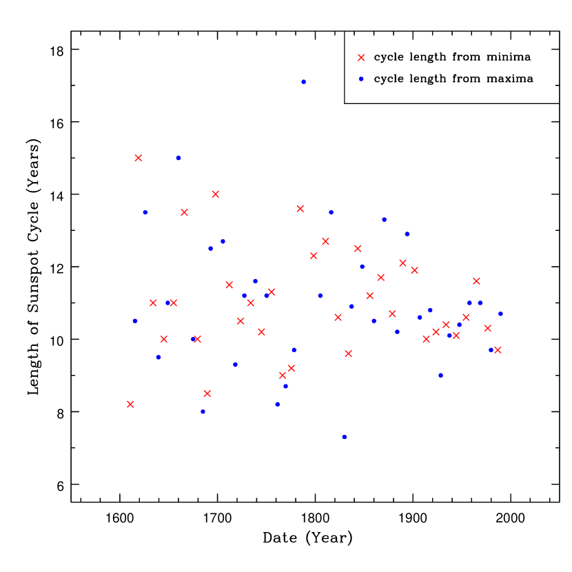
Figure 5.— Sunspot cycle durations derived from successive minima (crosses) and successive maxima (dots) for dates from 1610.8 to 1989.6.

4.1. Median Trace Analysis

Median trace analyses have been used to identify hidden trends in scatter plots which, at first glance, display no obvious pattern (e.g., Moore & McCabe 2005). These analyses have also been applied to astronomical data (e.g., Gott et al. 2001; Avelino et al. 2002; Chen & Ratra 2003; Chen et al. 2003). The method of median trace analysis is applicable to any scatter plot, irrespective of how measurements were obtained, and is one of a general class of smoothing methods designed to identify trends in scatter plots.

A median trace is a plot of the median value of the data contained within a bin of a chosen width, for all bins in the data set (Hoaglin et al., 1983). A median trace analysis depends on the choice of an optimal interval width (OIW). These OIWs, $h_{n}$, were calculated using three statistical methods applied routinely to estimate the statistical density function of the data. The first method defines the OIW as

$$h_{n,1}=\frac{3.49\,{\tilde{s}}}{n^{1/3}}$$ (1)

where $n$ is the number of data points and $\tilde{s}$, a statistically robust measure of the standard deviation of the data called the mean absolute deviation from the sample median, is defined as

$${\tilde{s}}=\frac{1}{n}~{}\sum_{i=1}^{n}|x_{i}-M|~{},$$ (2)

where $M$ is the sample median. The second method defines the OIW as

$$h_{n,2}=1.66\,{\tilde{s}}\left(\log_{e}n\over n\right)^{1/3}.$$ (3)

A third definition of the OIW is given by

$$h_{n,3}={2\times IQR\over n^{1/3}}~{},$$ (4)

where $IQR$ is the interquartile range of the data set. Optimal bin widths were determined for three data sets corresponding to the cycle lengths derived from the (i) cycle minima, (ii) cycle maxima, and (iii) the combined minima and maxima data. Table 4 lists the solutions for the optimal interval widths ($h_{n,1},h_{n,2},h_{n,3}$) for each data set.

Since the values of the optimal bin widths ranged from $\sim$60 – 120 years, we tested the impact of different bin widths on our results. This procedure was limited by the fact that only 35 sunspot number cycles have elapsed since 1610 (see Table 2). The data set can be increased to 70 points if we analyze the combined values of the length of the solar cycle derived from both the sunspot minima and the sunspot maxima. Using our derived OIWs as a basis for our analysis, we calculated median traces for bin widths of 40, 50, 60, 70, 80, and 90 years. These are illustrated in Figure 6. The lower bin widths were included to make maximum use of the limited number of data points, and the higher bin widths were excluded because, once binned, there would be too few data points to make those analyses meaningful.

Table 4Optimal Interval Widths

	Data	St. Dev.	Opt. Bin Width (yrs)
Data Set	$n$	$\tilde{s}$ (yrs)	$h_{n,1}$	$h_{n,2}$	$h_{n,3}$
Cycle Minima	35	97.4	103.9	75.4	116.6
Cycle Maxima	35	97.0	103.4	75.1	115.4
Combined	70	97.3	82.4	63.5	91.8

Figure 6 shows the binned data (median values) and the sinusoidal fits to the binned data. The Least Absolute Error Method (Bates & Watts, 1988) was used to produce the sinusoidal fits to the median trace in each frame of the figure. These sinusoidal fits illustrate the long-term cyclic behavior in the length of the sunspot number cycle. The optimal solution was determined by identifying the fits that satisfied two criteria: (1) the cycle periods deduced from the three data sets should be nearly the same, and (2) the cyclic patterns should be in phase for the three data sets. Table 5 lists the derived cycle periods for all three data sets: the (a) cycle minima, (b) cycle maxima, and (c) combined minima and maxima data.

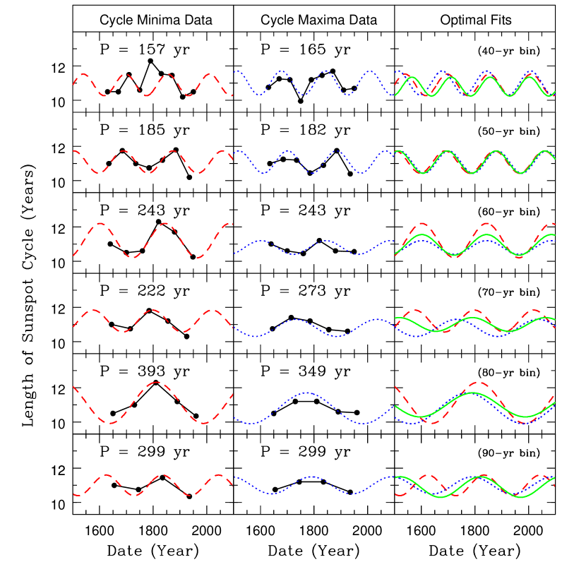
Figure 6.— Median traces for sunspot minima data (left column) and maxima data (middle column) derived for bin widths of 40 – 90 years. A sinusoidal fit to the median trace is shown for each bin width (minima-dashed line, maxima-dotted line, and combined maxima and minima-solid line). The average period of each derived sinusoidal fit is given at the top of each frame. The optimal fits (right column) show that the optimal bin width is in the range of 50 – 60 years because it is only in these two cases that the sinusoidal fits are in phase and the derived periods are approximately equal for all three data sets.

4.2. Results of Median Trace Analysis

The lengths of the sunspot number cycles tabulated by the National Geophysical Data Center (Table 2 & Figure 5) show that the basic sunspot number cycle is an average of (11.0 $\pm$ 1.5) years based on the cycle minima and (11.0 $\pm$ 2.0) years based on the cycle maxima. This Schwabe Cycle varies over a range from 8 to 15 years if the cycle lengths are derived from the time between successive minima, while the range increases to 7 to 17 years if the cycle lengths are derived from successive maxima. These variations may be significant even though the data in Figure 5 show heteroskedasticity, i.e., variability in the standard deviation of the data over time. Although the range in sunspot cycle durations is large, the cycle length converged to a mean of 11 years, especially after 1818 as the accuracy of the data became more reliable. In particular, the sunspot number cycle lengths from 1610 - 1750 had a high variance while the cycle durations since 1818 show a much smaller variance (Figure 5) because the data quality was poor in the 18th and early 19th century. This variance may be influenced by the difficulty in identifying the dates of cycle minima and maxima whenever the sunspot activity is relatively low. Even after the data became more accurate there was still a significant $\pm$ 1.5-year range about the 11-year mean. The range in the length of this cycle suggests that there may be a hidden longer-term variability in the Schwabe cycle.

Our median trace analysis of the lengths of the sunspot number cycle uncovered a long-term cycle with a duration between 146 and 419 years (Table 5), if the data are binned in groups of 40 to 90 years (see §4.1). Since the median trace analysis is influenced by the bin size of the data, we determined the optimal bin width based on the goodness of fit between the median trace and the corresponding sinusoidal fit (see Figure 6). Based on the sunspot minima (the best data set), the cycle length was 185 years for the 50-yr bin width, 243 years for the 60-yr bin, 222 years for the 70-yr bin, 393 years for the 80-year bin, and 299 years for the 90-yr bin; so we found no direct relationship between the bin size and the resulting periodicity. Figure 6 also shows the median traces for the data and illustrates that the optimal bin width is in the range of 50 - 60 years because it is only in these two cases that the sinusoidal fits are in phase and the derived periods are approximately equal for all three data sets. The 50-year median trace predicts a 183-year sunspot number cycle, while the 60-year trace predicts a 243-year cycle. Since the observations span $\sim$385 years, there is greater confidence in the 183-year cycle than in the longer one because at least two cycles have elapsed since 1610. Similar long-term cycles ranging from 169 to 189 years have been proposed for several decades (Kuklin, 1976).

Table 5Optimal Interval Widths

Bin Width	Derived Periodicities (yrs)
(yrs)	Minima	Maxima	Both	Average
40	157	165	146	156 $\pm$ 10
50	185	182	182	183 $\pm$ 2
60	243	243	243	243
70	222	273	304	266 $\pm$ 41
80	393	349	419	387 $\pm$ 35
90	299	299	209	269 $\pm$ 52

4.3. Analysis of the (O-C) Data

The median trace analysis gives us a rough estimate of the long-term sunspot cycle. However, an alternative method to derive this secular period is to calculate the power spectrum of the (O-C) variation of the dates corresponding to the (i) cycle minima, (ii) cycle maxima, and (iii) the combined minima and maxima.

The following procedure was used to calculate the (O-C) residuals for each of the data sets given above, based only on the dates of minima and maxima listed in Table 2. First, we defined the cycle number, $\phi$, to be $\phi=(t_{i}-t_{0})/L$, where $t_{i}$ are the individual dates of the extrema, and $t_{0}$ is the start date for each data set. Here, L is the average cycle length (10.95 years) derived independently by the FFT and PDM analyses from the sunspot number data (§3.2). The (O-C) residuals were defined to be

$$(O-C)=(t_{i}-t_{0})-(N_{c}\times L)$$

where, $N_{c}$ is the integer part of $\phi$ and represents the whole number of cycles that have elapsed since the start date. The resulting (O-C) pattern was normalized by subtracting the linear trend in the data. This trend was found by fitting a least squares line to the (O-C) data. The normalized (O-C) data are shown in Figure 7 along with the corresponding power spectra.

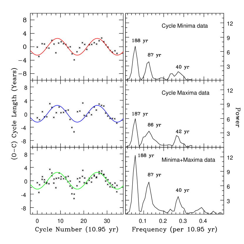
Figure 7.— The cycle length (O-C) residuals (left frames) and the corresponding power spectrum (right frames) derived from the sunspot cycle minima (top frame), maxima (middle frame), and combined minima and maxima data (bottom frame). The solid line through the data represents the long term cycle derived from the power spectrum analysis.

4.4. Results of (O-C) Data Analysis

The power spectra of the (O-C) data in Figure 7 show that the long term variation in the sunspot number cycle has a dominant period of $188\pm 38$ years. The Gleissberg cycle was also identified in this analysis, with a period of $87\pm 13$ years. The solutions for these analyses are illustrated in Figure 7 and tabulated in Table 6. The $1\sigma$ errors were calculated from the FWHM of the power spectrum peaks, as described in §3.2. The sinusoidal fit to the (O-C) data in Figure 7 corresponds to the dominant periodicity of 188 years identified in the power spectra. Another cycle with a period of $\sim 40$ years was also found.

Table 6Derived Long Term Solar Cycles

	Gleissberg	Secular
Data Set	(yrs)	(yrs)
Cycle Minima	86.8 $\pm$  8.8	188 $\pm$ 40
Cycle Maxima	86.3 $\pm$ 18.1	187 $\pm$ 37
Combined	86.8 $\pm$ 10.7	188 $\pm$ 38
Average	86.6 $\pm$ 12.5	188 $\pm$ 38

5. Discussion and Conclusions

Our study of the length of the sunspot cycle suggests that the cycle length should be taken into consideration when predicting the start of a new solar cycle. The variability in the length of the sunspot cycle was examined through a study of archival sunspot data from 1610 – 2005. In the preliminary stage of our study, we analyzed archival data of sunspot numbers from 1700 - 2005 and sunspot areas from 1874 - 2005 using power spectrum analysis and phase dispersion minimization. This analysis showed that the Schwabe Cycle has a duration of (10.80 $\pm$ 0.50) years (Table 3) and that this cycle typically ranges from $\sim$10 – 12 years even though the entire range is from $\sim$7 – 17 years. Based on our results, we have found evidence to show that (1) the variability in the length of the solar cycle is statistically significant. In addition, we predict that (2) the length of successive solar cycles will increase, on average, over the next 75 years; and (3) the strength of the sunspot cycle should eventually reach a minimum somewhere between Cycle 24 and Cycle 31, and we make no claims about any specific cycle.

The focus of our study was to investigate whether there is a secular pattern in the range of values for the Schwabe cycle length. We used our derived value for the Schwabe cycle from Table 3 to examine the long-term behavior of the cycle. This analysis was based on NGDC data from 1610–2000, a period of 386 years (using sunspot minima) or 385 years (using sunspot maxima). The long-term cycles were identified using median trace analyses of the length of the cycle and also from power spectrum analyses of the (O-C) residuals of the dates of sunspot minima and maxima. We used independent approaches because of the inherent uncertainties in deriving the exact times of minima and the even greater complexity in the determination of sunspot maxima. Moreover, we derived our results from both the cycle minima and the cycle maxima. The fact that we found similar results from the two data sets suggests that the methods used to determine these cycles (NGDC data) did not have any significant impact on our results.

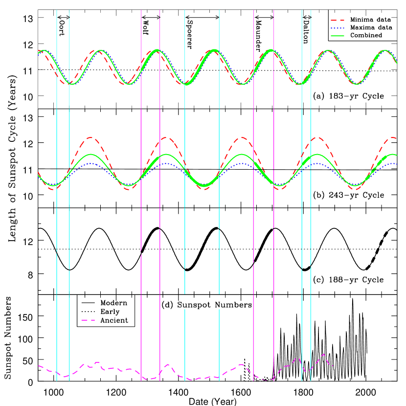
Figure 8.— Sinusoidal fits to the sunspot number cycle corresponding to the derived periods of (a) 183 years, (b) 243 years, and (c) 188 years, compared with (d) the sunspot number data. The fits to (a) and (b) were produced from binned cycle minima (dashed line), cycle maxima (dotted line), and a combination of the two data sets (solid line). The bottom frame shows sunspot numbers from 1700 – 2004 (modern, solid line), 1610 – 1715 (early, dotted line), and 950 – 1950 (ancient, dashed line) reconstructed from radiocarbon data. The 183- and 188-year periodicities display the best match to the historical minima.

The median trace analysis of the length of the sunspot number cycle provided secular periodicities of 183 – 243 years. This range overlaps with the long-term cycles of $\sim$90 – 260 years which were identified directly from the FFT and PDM analyses of the sunspot number and area data (Figures 3 and 4). The power spectrum analysis of the (O-C) residuals of the dates of minima and maxima provided much clearer evidence of dominant cycles with periods of $188\pm 38$ years, $87\pm 13$ years, and $\sim 40$ years. These results are significant because at least two long-term cycles have transpired over the $\sim$385-year duration of the data set.

The derived long-term cycles were compared in Figure 8 with documented epochs of significant declines in sunspot activity, like the Oort, Wolf, Spörer, Maunder, and Dalton Minima (Eddy, 1977; Stuiver & Quay, 1980; Siscoe, 1980). In this figure, the modern sunspot number data were combined with earlier data from 1610-1715 (Eddy, 1976) and with reconstructed (ancient) data spanning the past 11,000 years (Solanki et al., 2004). These reconstructed sunspot numbers were based on dendrochronologically-dated radiocarbon concentrations which were derived from models connecting the radiocarbon concentration with sunspot number (Solanki et al., 2004). The reconstructed sunspot numbers are consistent with the occurrences of the historical minima (e.g., Maunder Minimum). Solanki et al. (2004) found that over the past 70 years, the level of solar activity has been exceptionally strong. Our 188-year periodicity is similar to the 205-year de Vries-Seuss cycle which has been identified from studies of the carbon-14 record derived from tree rings (e.g., Wagner et al. 2001; Braun et al. 2005).

Figure 8 compares the historical and modern sunspot numbers with the derived secular cycles of length (a) 183 years (§4.2), (b) 243-years (§4.2), and (c) 188 years (§4.4). The first two periodicities were derived from the median trace analysis, while the third one was derived from the power spectrum analysis of the sunspot number cycle (O-C) residuals. The fits for the 183-year periodicity all had the same amplitude, but were moderately out of phase with each other, while the fits for the 243-year periodicity were in phase for all data sets, albeit with different amplitudes.

An examination of frames (a) and (c) of Figure 8 reveals that the cycle lengths increased during each of the Wolf, Spörer, Maunder, and Dalton Minima for the 183-year and 188-year cycles. On the other hand, frame (b) shows no similar correspondence between the cycle length and the times of historic minima for the 243-year cycle. Therefore, the 183- and 188-year cycles appear to be more consistent with the sunspot number data than the 243-year cycle. All four historic minima since 1200 occurred during the rising portion of the 183- and 188-year cycles when the length of the sunspot cycle was increasing. According to our analysis, the length of the sunspot cycle was growing during the Maunder Minimum when almost no sunspots were visible. Given this pattern of behavior, the next historic minimum should occur during the time when the length of the sunspot cycle is increasing (see Fig. 8).

The existence of long-term solar cycles with periods between 90 and 200 years is not new to the literature but the nature of these cycles is still not fully understood. Our study of the length of the sunspot cycle shows that there is a dominant periodicity of 188 years related to the basic Schwabe Cycle and weaker periodicities of $\sim$40 and 87 years. This 188-year period, determined over a baseline of 385 years that spans more than two cycles of the long-term periodicity, should be compared with Schwabe’s 10-year period that was derived from 17 years (i.e., less than two cycles) of observations (Schwabe, 1844). Our study also suggests that the length of the sunspot number cycle should increase gradually, on average, over the next $\sim$75 years, accompanied by a gradual decrease in the number of sunspots. This information should be considered in cycle prediction models (e.g., Dikpati, de Toma & Gilman 2006) to provide better estimates of the starting time of a given cycle.

References

- Avelino et al. (2002) Avelino, P. P., Martins, C. J. A. P., & Pinto, P. 2002, ApJ, 575, 989
- Balasubramaniam & Regan (1994) Balasubramaniam, K. S. & Regan, J. 1994, in Solar Active Region Evolution - Comparing Models with Observations, eds. K. S. Balasubramaniam & G. Simon, ASP Conf. Ser., 68, 17 (San Francisco: ASP)
- Bevington (1969) Bevington, P. R. 1969, Data Reduction and Error Analysis for the Physical Sciences (New York: McGraw-Hill)
- Baliunas & Vaughan (1985) Baliunas, S. L., Vaughan, A. H. 1985, ARA&A, 23, 379
- Bates & Watts (1988) Bates, D. M. & Watts, D. G. 1988, Nonlinear Regression Analysis and Its Applications (New York: Wiley)
- Biesecker (2007) Biesecker, D. A. 2007, BAAS, 38, p.209
- Braun et al. (2005) Braun, H., Christi, M., Rahmstorf, S., Ganopolski, A., Mangini, A., Kubatzki, C., Roth, K., & Kromer B. 2005, Nat, 438, 208
- Chen & Ratra (2003) Chen, G. & Ratra, B. 2003, PASP 115, 1143
- Chen et al. (2003) Chen, G., Gott, J. R., & Ratra, B. 2003, PASP 115, 1269
- Coffey & Erwin (2004) Coffey, H. E., and Erwin, E. 2004, National Geophysical Data Center, NOAA (ftp://ftp.ngdc.noaa.gov/STP/ SOLAR DATA/SUNSPOT NUMBERS; www.ngdc.noaa .gov/stp/SOLAR/ftpsunspotnumber.html#international; www.ngdc.noaa.gov/stp/SOLAR/ftpsunspotregions.html)
- de Toma et al. (2004) de Toma, G., White, O. R., Chapman, G. A., Walton, S. R., Preminger, D. G., & Cookson, A. M. 2004, ApJ, 609, 1140
- Dikpati, de Toma & Gilman (2006) Dikpati, M., de Toma, G., & Gilman, P. 2006, Geophys. Research Lett., 33, 5102
- Eddy (1976) Eddy, J. A. 1976, Science, 192, 1189
- Eddy (1977) Eddy, J. A. 1977, The Solar Output and Its Variation, ed. O. R. White, p. 51 (Boulder: Colorado Associated University Press)
- Elling & Schwentek (1992) Elling, W. & Schwentek, H. 1992, Solar Phys., 137, 155
- Gott et al. (2001) Gott, J. R., Vogeley, M.S., Podariu, S., & Ratra, B. 2001, ApJ, 549, 1
- Hathaway (2004) Hathaway, D. H. 2004, Royal Greenwich Obs./USAF/noaa, Sunspot Record 1874-2004, NASA/Marshall Space Flight Center
- Hoaglin et al. (1983) Hoaglin, D., Mosteller, F., & Tukey, J. 1983, Understanding Robust and Exploratory Data Analysis (New York: Wiley)
- Hoyt & Schatten (1998) Hoyt, D. V. & Schatten, K. H. 1998, Solar Phys., 179, 189
- Joselyn et al. (1996) Joselyn, J. A., Anderson, J., Coffey, H., Harvey, K., Hathaway, D., Heckman, G., Hildner, E., Mende, W., Schatten, K., Thompson, R., Thomson, A. W. P., & White, O. R. 1996, Solar Cycle 23 Project: Summary of Panel Findings (http://www.sec.noaa.gov/info/Cycle23.html)
- Kilcik et al. (2009) Kilcik, A., Anderson, C. N. K., Rozelot, J. P., Ye, H., Sugihara, G., & Ozguc, A. 2009, ApJ, 693, 1173
- Kuklin (1976) Kuklin, G. V. 1976, Basic Mechanisms of Solar Activity, IAU Symp. No. 71, ed. V. Bumba, J. Kleczek, p. 147 (Boston: Reidel)
- Li et al. (2005) Li, K. J., Qiu, J., Su, T. W., & Gao, P.X. 2005, ApJ, 621, L81
- Lupton & Monger (1977) Lupton, R., & Monger, P. 1977, The SuperMongo Reference Manual, (http://www.astro.princeton.edu/r̃hl/sm/)
- Maunder (1904) Maunder, E. W. 1904, MNRAS, 64, 747
- Moore & McCabe (2005) Moore, D. & McCabe, G. 2005, Introduction to the Practice of Statistics, 5th ed. (New York: Freeman)
- Press et al. (1992) Press, W. H., Teukolsky, S. A., Vetterling, W. T., & Flannery, B. P. 1992, Numerical Recipes in FORTRAN: The Art of Scientific Computing (Cambridge: Cambridge University Press), 2nd edition.
- Richards, Waltman, Ghigo, & Richards (2003) Richards, M. T., Waltman, E. B., Ghigo, F., & Richards, D. St. P. 2003, ApJS, 147, 337
- Rogers & Richards (2004) Rogers, M. L., & Richards, M. T. 2004, BAAS, 36, 670
- Rogers, Richards, & Richards (2006) Rogers, M. L., Richards, M. T., & Richards, D. St. P. 2006, astro-ph/0606426
- Schwabe (1844) Schwabe, M. 1844, Astron. Nach., 21, 233
- Siscoe (1980) Siscoe, G. L. 1980, Rev. Geophys. Space Phys., 18, 647
- Solanki et al. (2004) Solanki, S. K., Usoskin, I.G., Kromer, B., Schüssler, M., & Beer, J. 2004, Nat, 431, No. 7012, p. 1084
- Stellingwerf (1978) Stellingwerf, R. F. 1978, AJ, 224, 953
- Stuiver & Quay (1980) Stuiver, M., & Quay, P. D. 1980, Sci, 207, 11
- Topping (1972) Topping, J. 1972, Errors of Observation and Their Treatment (London: Chapman & Hall)
- Usoskin & Mursula (2003) Usoskin, I. G., & Mursula, K. 2003, Solar Phys., 218, 319
- Wagner et al. (2001) Wagner, G., Beer, J., Masarik, J., Muscheler, R., Kubik, P., Mende, W., Laj, C., Raisbeck, G., & Yiou, F. 2001, Geophys. Research Lett., 28, 303
- Waldmeier (1961) Waldmeier, M. 1961, The Sunspot Activity in the Years 1610-1960 (Zurich: Zurich Schulthess and Co. AG)
- Wilson (2006) Wilson, I. R. G. 2006, Proceedings of Australian Inst. Phys., 17th National Congress, Brisbane, 3-8 December 2006
- Wilson et al. (2008) Wilson, I. R. G., Carter, B. D., & Waite, I. A. 2008, Publ. Astron. Soc. Australia, 25, 85
- Wilson (1994) Wilson, P. R. 1994, Solar and Stellar Activity Cycles (New York: Cambridge University Press)
- Wilson (1987) Wilson, R. M. 1987, J. Geophys. Res., 92, 10101