Frequency dependence of the Chiral Vortical Effect

Abstract

We study the frequency dependence of all the chiral vortical and magnetic conductivities for a relativistic gas of free chiral fermions and for a strongly coupled conformal field theory with holographic dual in four dimensions. Both systems have gauge and gravitational anomalies, and we compute their contribution to the conductivities. The chiral vortical conductivities and the chiral magnetic conductivity in the energy current show a frequency dependence in the form of a delta centered at zero frequency. This highly discontinuous behavior is a natural consequence of the Ward identities that include the energy momentum tensor. We discuss the physical interpretation of this result and its possible implications for the quark gluon plasma as created in heavy ion collisions. In the Appendix we discuss why the chiral magnetic effect seems to vanish in the consistent current for a particular implementation of the axial chemical potential.

I Introduction

During the last years the study of anomaly induced transport coefficients has proved a subject of increasing interest. Charge separation found in RHIC and confirmed more recently at the LHC Abelev et al. (2009, 2013) can possibly be traced back to the chiral magnetic Effect (CME). This effect says that a system with triangle anomalies in an external magnetic field will show an electric current parallel to the magnetic field Fukushima (2013)

$$\vec{J}=\frac{e\mu_{5}}{2\pi^{2}}e\vec{B}.$$ (1)

There have been early precursors that studied manifestation of this phenomena in neutrino physics Vilenkin (1995, 1980a), the early universe Giovannini and Shaposhnikov (1998) and condensed matter systems Alekseev et al. (1998). In recent years the increasing interest in this effect has been spurred by the role it might play in the physics of the quark gluon plasma.

But this phenomenon is not the only one present in a chiral system at finite temperature and/or chemical potential. The presence of a magnetic field can also produce an axial current known as the chiral separation effect (CSE) Son and Zhitnitsky (2004); Metlitski and Zhitnitsky (2005); Newman and Son (2006) and a vortex can contribute to the electric and axial current, this is the so-called chiral vortical effect (CVE) Kharzeev and Zhitnitsky (2007); Erdmenger et al. (2009); Banerjee et al. (2011); Son and Surowka (2009). Apart from charge flow in a relativistic fluid there exists also energy flow and analogous anomaly related transport effects in the energy current $J^{i}_{\epsilon}=T^{0i}$. In this paper we will use the compact notation $J^{i}_{A}\in\{J^{i}_{e},J^{i}_{5},J^{i}_{\epsilon}\}$, where we include the electric, axial and energy currents. With this notation we can write two compact Kubo formulae for the chiral magnetic and vortical conductivities Kharzeev and Warringa (2009); Amado et al. (2011); Landsteiner et al. (2013).

$$\sigma^{\cal B}_{A}(\omega,\vec{k})=-\sum_{i,j}\epsilon_{ijn}\frac{i}{2k_{n}}\langle J^{i}_{A}J^{j}_{e}\rangle\,,$$ (2)

$$\sigma^{\cal V}_{A}(\omega,\vec{k})=-\sum_{i,j}\epsilon_{ijn}\frac{i}{2k_{n}}\langle J^{i}_{A}J^{j}_{\epsilon}\rangle\,.$$ (3)

The most significant result of anomalies is that they produce equilibrium currents. These equilibrium conductivities are defined via the Kubo formulae in the kinematic region in which first the frequency is set to zero and then the limit to zero momentum is taken.

As the quark gluon plasma produced in a heavy ion collision has a finite life time and size, it is mandatory to know the full frequency and momentum dependence of the response to magnetic field and vorticity. A detailed study of the frequency dependence of the chiral magnetic effect at weak coupling was done in Kharzeev and Warringa (2009) and in a strongly coupled regime using holography in Yee (2009). In the study of the chiral vortical conductivity in a static situation using Kubo formulae at weak coupling a surprising result was found Landsteiner et al. (2011a). A purely temperature dependent term appeared in the conductivity consistent with previous hydrodynamical analysis, but it was realized that this contribution is present if and only if the theory has a mixed gauge-gravitational anomaly. To verify that result at strong coupling a bottom up holographic model was built introducing a mixed gauge-gravitational anomaly into the system and the same contribution appeared in this holographic setup Landsteiner et al. (2011b). Actually this result has been confirmed many times using different approaches Loganayagam and Surowka (2012); Chapman et al. (2012); Gao et al. (2012); Jensen et al. (2013a); Megias and Pena-Benitez (2013a); Megias et al. (2013); Megias and Pena-Benitez (2013b). Anomalous conductivities are therefore sensitive to both, pure gauge and mixed gauge-gravitational anomalies. It is understood by now that in theories in which the anomaly is purely classical, e.g. neither the gauge fields nor the metrics are considered quantum variables, the anomalous equilibrium transport is subject to a non-renormalization theorem Son and Surowka (2009); Jensen et al. (2013a); Golkar and Son (2012); Gorbar et al. (2013); Hou et al. (2012); Zakharov (2013); Jensen et al. (2013b) .

A computation of the frequency dependence of the CVE was done in Amado et al. (2011) within a holographic model with a pure gauge anomaly only. However the contribution of the gravitational anomaly could be a leading term in heavy ion collisions where the temperature reached is much higher than the chemical potential. Therefore it is necessary to consider both anomalies. In the experiment the charge separation due to the CME and CVE in the vector current should be seen through the search of charged particles in the perpendicular directions to the reaction plane Kharzeev and Son (2011). And the signature left by the separation of chirality is predicted to be an enhanced production of higher spin mesons after the freezeout Keren-Zur and Oz (2010).

As we previously said a more realistic analysis of the CVE is needed. We take this as the motivation to compute the frequency and momentum dependence of the chiral vortical conductivity in the electric, axial and energy currents at weak and strong coupling.

At weak coupling this implies working out the sum over Matsubara frequencies. We take this as an opportunity to give a careful discussion of the seeming “gauge” dependence on the result for the CME in the Appendix. It is well established Rebhan et al. (2010); Landsteiner et al. (2013); Jensen et al. (2013a) that the CME receives an additional contribution depending on the axial gauge potential if formulated in terms of the consistent current. We show how this appears at weak coupling and we give a physical interpretation to the different responses in consistent and covariant currents.

The manuscript is organized as follows. In section II we consider a gas of free fermions with a $U(1)_{V}\times U(1)_{A}$ global symmetry and compute the frequency and momentum dependence of all the anomaly induced transport coefficients using Kubo formulae. We present in section III a numerical computation of the conductivities using a holographic model describing a strongly coupled plasma of fermions with the same symmetry group as in the weakly coupled case. In section IV we compute the anomalous transport predicted by hydrodynamics, and compare with the strong coupling results. Finally we discuss the role of the CVE in heavy ion collisions and draw our conclusions in section VI. In the Appendix we discuss the subtleties arising in the sum over Matsubara frequencies when dealing with chemical potentials for anomalous symmetries.

II Weakly coupled regime

We define the chemical potential through boundary conditions on the fermion fields around the thermal circle Landsman and van Weert (1987), $\Psi^{f}(\tau)=-e^{\beta\mu^{f}}\Psi^{f}(\tau-\beta)$ with $\beta=1/T$. Therefore the eigenvalues of $\partial_{\tau}$ are $i\tilde{\omega}_{n}+\mu^{f}$ for the fermion species $f$ with $\tilde{\omega}_{n}=\pi T(2n+1)$ the fermionic Matsubara frequencies. From now on we will consider the symmetry group $U_{V}(1)\times U_{A}(1)$, i.e. one vector and one axial current with chemical potentials $\mu_{\pm}=\mu\pm\mu_{5}$, charges $q^{+}_{v,5}=(1,1)$ and $q^{-}_{v,5}=(1,-1)$ for one right-handed and one left-handed fermion. A convenient way of expressing the currents is in terms of Dirac fermions and writing

$$J^{i}_{e,5}(x) = \bar{\Psi}(x)\gamma^{i}Q_{e,5}\Psi(x)\,,$$ (4)

$$J^{i}_{\epsilon}(x) = \frac{i}{4}\bar{\Psi}(x)(\gamma^{0}\overleftrightarrow{\partial^{i}}+\gamma^{i}\overleftrightarrow{\partial^{0}})\Psi(x)\,,$$ (5)

where the vector charge is $Q_{e}={\mathcal{P}}_{+}+{\mathcal{P}}_{-}$ and the axial charge is $Q_{5}=\mathcal{P}_{+}-\mathcal{P}_{-}$. $J_{e}$, $J_{5}$ and $J_{\epsilon}$ correspond to the vector, axial and energy currents, respectively. We used the chiral projector ${\cal P}_{\pm}=\frac{1}{2}(1\pm\gamma_{5})$. Our metric is $g_{\mu\nu}=\operatorname{diag}(1,-1,-1,-1)$. The fermion propagator is

$$S(q) = \frac{1}{2}\sum_{s,t=\pm}\Delta_{t}(i\tilde{\omega}_{s},\vec{q}){\cal P}_{s}\gamma_{\mu}\hat{q}^{\mu}_{t}\,,$$ (6)

$$\Delta_{t}(i\tilde{\omega}_{s},q) = \frac{1}{i\tilde{\omega}_{s}-tE_{q}}\,,$$ (7)

with $i\tilde{\omega}_{s}=i\tilde{\omega}_{n}+\mu_{s}$, $\hat{q}_{t}^{\mu}=(1,t\hat{q})$, $\hat{q}=\frac{\vec{q}}{E_{q}}$. We will consider massless fermions, so that $E_{q}=|\vec{q}|$. The value $t=+1$ corresponds to particles (positive energy) and $t=-1$ to antiparticles (negative energy). Label $s$ refers to right-handed ($s=+1$) and left-handed ($s=-1$) chiralities, so that right and left chemical potentials are related to baryon and axial chemical potentials as $\mu_{s}=\mu+s\mu_{5}$.

II.1 Chiral vortical conductivities

Since we have the Kubo formulae, the problem of computing the transport coefficients, Eqs. (2) and (3), reduces to the computation of the retarded correlator between the currents $J_{A}^{i}$

$$G_{AB}(x-x^{\prime})=\frac{1}{2}\epsilon_{ijn}\,i\,\theta(t-t^{\prime})\,\langle[J^{i}_{A}(x),J^{j}_{B}(x^{\prime})]\rangle\,,$$ (8)

in particular we will focus on the case of the vortical conductivity in which the second current in the formula (8) is the energy flux $J^{i}_{\epsilon}$. The generalization to the magnetic case is straightforward, and we will address it in Sec. II.2. Let us redefine the correlators associated with the chiral vortical effect as

$$G_{A}^{\cal V}\equiv G_{A\epsilon}\,,\qquad A=e,5,\epsilon\,.$$ (9)

The one loop correlators $G_{5}^{\cal V}$ and $G_{\epsilon}^{\cal V}$ can be computed, respectively, as

Figure 1: One loop diagram contributing to the chiral vortical conductivities $G_{A}^{\cal V}$, see Eqs. (10) and (11). For $A=\epsilon$ there is also the contribution coming from the seagull diagram, see Manes and Valle (2013).

$$G_{5}^{\cal V}(k_{0},k) = \frac{1}{8\beta}\sum_{\tilde{\omega}}\int\frac{d^{3}q}{(2\pi)^{3}}\epsilon_{ijn}\operatorname{tr\>}\Bigg{[}S(q)\gamma^{i}\gamma_{5}S(q+k)\left(\gamma^{0}(2q^{j}+k^{j})+\gamma^{j}(2i\tilde{\omega}+k^{0})\right)\Bigg{]}\,,$$ (10)

$$G_{\epsilon}^{\cal V}(k_{0},k)=\frac{1}{16\beta}\sum_{\tilde{\omega}}\int\frac{d^{3}q}{(2\pi)^{3}}\epsilon_{ijn}\operatorname{tr\>}\Bigg{[}S(q)\gamma^{i}S(q+k)\left(2\gamma^{0}(2q^{j}+k^{j})+\gamma^{j}(2i\tilde{\omega}+k^{0})\right)(2i\tilde{\omega}+k^{0})+S(q)\left\{\gamma^{i}\gamma^{j},k\!\!\!\!/\right\}\Bigg{]}\,,$$ (11)

where $k\!\!\!\!/=\gamma^{\mu}k_{\mu}=\gamma^{0}k^{0}-\gamma^{m}k^{m}$. Figure 1 shows the one loop diagram corresponding to $G_{A}^{\cal V}$. The expression for $G_{e}^{\cal V}(k_{0},k)$ is the same as Eq. (10) but removing the $\gamma_{5}$ matrix in the integrand. The last term inside the bracket in Eq. (11) corresponds to the seagull diagram which was computed in Manes and Valle (2013). The correlators $G_{e}^{\cal V}(k_{0},k)$ and $G_{5}^{\cal V}(k_{0},k)$ have been computed in detail in Ref. Landsteiner et al. (2011a) at zero frequency, and the computation of $G_{\epsilon}^{\cal V}(k_{0},k)$ follows straightforwardly by using the same procedure, so we will skip here the technical details. An evaluation of Eqs. (10) and (11) leads to the result (from now on we denote $q=|\vec{q}|$ and $k=|\vec{k}|$)

$$\widehat{G}_{A}^{\cal V}(k_{0},k)=\frac{ik_{n}}{16\pi^{2}}\int_{0}^{\infty}dq\,f_{A}^{\cal V}(q)g_{A}^{\cal V}(q)\,,$$ (12)

where

$$g_{A}^{\cal V}(q)=\left\{\begin{array}[]{ll}q\left(1-3\frac{k_{0}^{2}}{k^{2}}\right)+\frac{(k^{2}-k_{0}^{2})}{8k^{3}}\sum_{t=\pm}\left[3k_{0}^{2}-k^{2}+12q(q+k_{0}t)\right]\log\left[\frac{\Omega_{t}^{2}-(q+k)^{2}}{\Omega_{t}^{2}-(q-k)^{2}}\right]&A=e,5\\ 2q^{2}\left(1-2\frac{k_{0}^{2}}{k^{2}}\right)+\frac{(k^{2}-k_{0}^{2})}{16k^{3}}\sum_{t=\pm}(2q+k_{0}t)(2k_{0}^{2}-k^{2}+8q(q+k_{0}t))\log\left[\frac{\Omega_{t}^{2}-(q+k)^{2}}{\Omega_{t}^{2}-(q-k)^{2}}\right]&A=\epsilon\end{array}\right.$$ (13)

with $\Omega_{t}=k_{0}+i\epsilon+tq$, and

$$f_{A}^{\cal V}(q)=\sum_{s,t=\pm}s^{\alpha}t^{\gamma}n(E_{q}-t\mu_{s})\,,\qquad\left\{\begin{array}[]{l}\alpha=1,\gamma=0\quad,\quad A=e\\ \alpha=0,\gamma=0\quad,\quad A=5\\ \alpha=1,\gamma=1\quad,\quad A=\epsilon\end{array}\right.\,,$$ (14)

where $n(x)=1/(e^{\beta x}+1)$ is the Fermi-Dirac distribution function. The hat in Eq. (12) denotes the vacuum subtracted contribution (see the Appendix). To compute the imaginary part of Eqs. (12) and (refeq:gAV) in the same spirit of Kharzeev and Warringa (2009) we need the relations

$$\mathop{\rm Im}\sum_{t=\pm}\log\left[\frac{(k_{0}+i\epsilon+tq)^{2}-(k+q)^{2}}{(k_{0}+i\epsilon+tq)^{2}-(k-q)^{2}}\right]= \pi\,\left[\theta(k_{+}-q)-\theta(k_{-}-q)\right]\,,$$ (15)

$$\mathop{\rm Im}\sum_{t=\pm}t\log\left[\frac{(k_{0}+i\epsilon+tq)^{2}-(k+q)^{2}}{(k_{0}+i\epsilon+tq)^{2}-(k-q)^{2}}\right]= -\pi\,\theta(k_{0}^{2}-k^{2})\,\mathrm{sgn}(k_{0})\,\left[\theta(k_{+}-q)-\theta(k_{-}-q)\right]+\,$$

$$+\pi\,\theta(k^{2}-k_{0}^{2})\,\left[\theta(q-k_{+})+\theta(q-k_{-})\right]\,,$$ (16)

where $\theta(x)$ is the step function and $k_{\pm}=\frac{1}{2}|k_{0}\pm k|$. From an analytical evaluation of Eqs. (12) and (13) for $A=e,5,\epsilon$ one gets the following momentum and frequency dependence of the vector, axial and energy vortical conductivities,

$$\mathop{\rm Im}[\sigma^{\cal V}_{A}(k_{0},k)] = \frac{1}{16\pi}\frac{k^{2}-k_{0}^{2}}{4k^{3}}\bigg{\{}2k_{0}\theta(k^{2}-k_{0}^{2})\left[24\mu\mu_{5}\delta_{A,e}+\left(12\left(\mu^{2}+\mu_{5}^{2}+\frac{\pi^{2}}{3}T^{2}\right)+(k_{0}^{2}-k^{2})\right)\delta_{A,5}\right]$$ (17)

$$-T\sum_{r,s,t=\pm}rs^{\alpha}\bigg{[}k^{2}\log{\left[1+{\mathrm{e}}^{\beta(k_{r}+t\mu_{s})}\right]}-12T^{2}\text{Li}_{3}\left(-e^{\beta(k_{r}+t\mu_{s})}\right)$$

$$+6kT\mathrm{Li}_{2}\left(-{\mathrm{e}}^{\beta(k_{r}+t\mu_{s})}\right)\left(\theta(k^{2}-k_{0}^{2})+r\operatorname{sign}(k_{0})\theta(k_{0}^{2}-k^{2})\right)\bigg{]}\bigg{\}}\,,\qquad A=e,5\,,$$

$$\mathop{\rm Im}[\sigma^{\cal V}_{\epsilon}(k_{0},k)] = \frac{1}{16\pi}\frac{k^{2}-k_{0}^{2}}{16k^{3}}\bigg{\{}8k_{0}\mu_{5}\theta(k^{2}-k_{0}^{2})\left[8(3\mu^{2}+\mu_{5}^{2})+\left(2k_{0}^{2}-k^{2}+2(2\pi T)^{2}\right)\right]+$$

$$\sum_{r,s,t=\pm}rst\bigg{[}10k^{2}T^{2}\text{Li}_{2}\left(-e^{\beta(k_{r}+t\mu_{s})}\right)+96T^{4}\text{Li}_{4}\left(-e^{\beta(k_{r}+t\mu_{s})}\right)$$

$$+kT\left(k^{2}\log{\left[1+{\mathrm{e}}^{\beta(k_{r}+t\mu_{s})}\right]}-48T^{2}\mathrm{Li}_{3}\left(-{\mathrm{e}}^{\beta(k_{r}+t\mu_{s})}\right)\right)\left(\theta(k^{2}-k_{0}^{2})+r\operatorname{sign}(k_{0})\theta(k_{0}^{2}-k^{2})\right)\bigg{]}\bigg{\}}\,,$$

where $\text{Li}_{n}(x)$ is the polylogarithm function of order $n$. A series expansion at small $k$ of these expressions leads to

$$\mathop{\rm Im}[\sigma^{\cal V}_{A}(k_{0},k)] = \theta(k^{2}-k_{0}^{2})\frac{1}{16\pi}\frac{k^{2}-k_{0}^{2}}{4k^{3}}k_{0}\bigg{[}24\mu\mu_{5}\delta_{A,e}+\left[12\left(\mu^{2}+\mu_{5}^{2}+\frac{\pi^{2}}{3}T^{2}\right)+(k_{0}^{2}-k^{2})\right]\delta_{A,5}$$ (19)

$$+\mu_{5}\left[8(3\mu^{2}+\mu_{5}^{2}+\pi^{2}T^{2})+\left(2k_{0}^{2}-k^{2}\right)\right]\delta_{A,\epsilon}\bigg{]}$$

$$-k^{2}\theta(k_{0}^{2}-k^{2})\frac{k_{0}|k_{0}|}{2^{10}\times 15\pi}\sum_{s,t=\pm}s^{\alpha}t^{\gamma}\left(\frac{d}{dx}\right)^{2-\gamma}n(2x-t\mu_{s})\Bigg{|}_{x=\frac{1}{4}|k_{0}|}+{\cal O}(k^{4})\,.$$

Notice that an expansion at small $k$ in the term $\sim\theta(k^{2}-k_{0}^{2})$ demands that one considers $|k_{0}|\lesssim k$, otherwise this contribution is vanishing. This restriction does not apply in the term $\sim\theta(k_{0}^{2}-k^{2})$. In the limit $k\to 0$ this expression leads to the result

$$\mathop{\rm Im}[\sigma_{A}^{\cal V}(\omega,0)]=\pi\sigma_{A,(0)}^{\cal V}\omega\delta(\omega)\,,\qquad\sigma_{A,(0)}^{\cal V}=\left\{\begin{array}[]{l}\frac{1}{2\pi^{2}}\mu\mu_{5}\\ \frac{1}{4\pi^{2}}\left(\mu^{2}+\mu_{5}^{2}+\frac{\pi^{2}}{3}T^{2}\right)\\ \frac{\mu_{5}}{6\pi^{2}}\left(3\mu^{2}+\mu_{5}^{2}+\pi^{2}T^{2}\right)\end{array}\right.\,,$$ (20)

where we have made use of the fact that $\lim_{k\to 0}\theta(k^{2}-k_{0}^{2})\frac{k^{2}-k_{0}^{2}}{k^{3}}=\frac{4}{3}\delta(k_{0})$. In Eq. (20) we have denoted the frequency as $\omega$. In the following we will use either $k_{0}$ or $\omega$. Using the Kramers-Kronig relation one can obtain the real part of the conductivities at $k=0$ and $\omega$ finite, and they read

$$\mathop{\rm Re}[\sigma_{A}^{\cal V}(\omega,0)]=\left\{\begin{array}[]{ll}\sigma_{A,(0)}^{\cal V}&\quad\omega=0\\ 0&\quad\omega\neq 0\end{array}\right.\,.$$ (23)

It is remarkable that the chiral vortical conductivities in the free field theory are zero at finite frequency and zero momentum. The discontinuous behavior at $\omega=0$ is also of great relevance. We show in fig. 2 the full frequency and momentum dependence of $\mathop{\rm Re}[\sigma^{\cal V}_{e}(\omega,k)]$ at low and high temperatures. We have introduced the dimensionless parameter $\tau=2\pi T/\mu$ in order to have a better comparison with the results from holography in Sec. III, variables. The figures have three features: i) at high temperature, there is a peak at $\omega=k$, ii) at low temperature, in addition to the peak at $\omega=k$, there are peaks at $\omega=k\pm 2\mu_{s}$, iii) the conductivities are vanishing at $k=0$, $\omega\neq 0$, and they present a discontinuity at $k=0$, $\omega=0$. From their behavior and these features one can see that the vortical conductivities are approximately vanishing at high temperature, in the regime $\omega>k$, see fig. 2. We will confront these results with the ones predicted at strong coupling in Sec. III, and discuss their implications in Sec. VI.

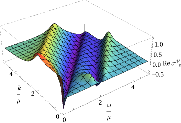
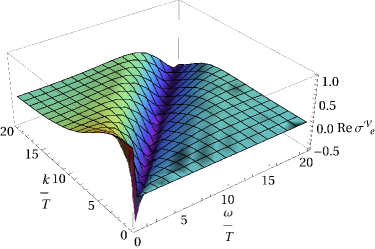
Figure 2: Frequency and momentum dependence of the real part of the vector vortical conductivity $\sigma_{e}^{\cal V}(\omega,k)$ normalized to its zero frequency-momentum value, from a numerical evaluation of Eqs. (12) and (14). We consider $\mu=10\,\textrm{MeV}$, $\mu_{5}=1\,\textrm{MeV}$, and temperature below the QCD phase transition $\tau=0.24$ (left figure) and above the phase transition $\tau=440$ (right figure). [Color online]

II.2 Chiral magnetic conductivity and chiral separation effect

We will extend for completeness the computation of the finite frequency and momentum behavior of conductivities to the chiral magnetic and separation effects. The chiral magnetic conductivity was studied in Kharzeev and Warringa (2009) in the case of a $U(1)_{V}\times U(1)_{A}$ symmetry at weak coupling. For a general symmetry group all the DC magnetic conductivities were computed in Landsteiner et al. (2011a). They follow from the retarded Green’s function of two charge currents

$$G_{A}^{\cal B}(x-x^{\prime})=\frac{1}{2}\epsilon_{ijn}\,i\,\theta(t-t^{\prime})\,\langle[J^{i}_{A}(x),J_{e}^{j}(x^{\prime})]\rangle\,,\qquad A=e,5,\epsilon\,.$$ (24)

Following a similar procedure as in the chiral vortical computation of Sec. II.1, we get that the retarded correlator can be written as

$$\widehat{G}^{{\cal B}}_{A}(k_{0},k) = \frac{i}{16\pi^{2}}\frac{k_{n}}{k}\frac{k^{2}-k_{0}^{2}}{k^{2}}\int_{0}^{\infty}dq\,f_{A}^{\cal B}(q)\sum_{t=\pm}(2q+k_{0}t)\log\left[\frac{\Omega_{t}^{2}-(q+k)^{2}}{\Omega_{t}^{2}-(q-k)^{2}}\right]\,,$$ (25)

where

$$f_{A}^{\cal B}(q)=\sum_{s,t=\pm}s^{\alpha}t\,n(E_{q}-t\mu_{s})\,,\qquad A=e,5\,,$$ (26)

and the value of $\alpha$ is defined as in Eq. (14). We do not show in Eqs. (25) and (26) explicit formulas for $G_{\epsilon}^{\cal B}(k_{0},k)$, as in the free field theory they are identical to $G_{e}^{\cal V}(k_{0},k)$, which was presented in Eqs. (12) and (refeq:fAV). This can easily be checked from the structure of the correlation functions, c.f. Eq. (10).

The frequency dependence for $\sigma^{\cal B}_{e}$ was originally computed in Kharzeev and Warringa (2009). Here we provide analytical results for this and other conductivities. In a series expansion at small $k$, the imaginary part writes

$$\mathop{\rm Im}[\sigma^{\cal B}_{A}(k_{0},k)] = \theta(k^{2}-k_{0}^{2})\frac{k^{2}-k_{0}^{2}}{4\pi k^{3}}k_{0}\left[\mu_{5}\delta_{A,e}+\mu\delta_{A,5}+\frac{3}{2}\mu\mu_{5}\delta_{A,\epsilon}\right]$$ (31)

$$+\theta(k_{0}^{2}-k^{2})\frac{k_{0}|k_{0}|}{96\pi}\sum_{s,t=\pm}t\zeta_{A}\left[\frac{d}{dx}+k^{2}\left(\frac{1}{k_{0}^{2}}\frac{d}{dx}+\frac{1}{40}\frac{d^{3}}{dx^{3}}\right)\right]n(x+t\mu_{s})\bigg{|}_{x=|k_{0}|/2}+{\cal O}(k^{4})\,,\quad\zeta_{A}=\left\{\begin{array}[]{l}s\\ 1\\ 0\end{array}\right.\,.$$

In the limit $k\to 0$ this expression leads to

$$\mathop{\rm Im}[\sigma^{\cal B}_{A}(\omega,0)]=\left(2+\delta_{A,\epsilon}\right)\frac{\pi}{3}\sigma^{\cal B}_{A,(0)}\omega\delta(\omega)+\frac{\omega|\omega|}{96\pi}\sum_{s,t=\pm}t\zeta_{A}\left[\frac{d}{dx}n(x+t\mu_{s})\right]_{x=|\omega|/2}\,,$$ (32)

where $\sigma^{\cal B}_{A,(0)}$ are given by

$$\sigma^{\cal B}_{A,(0)}=\frac{1}{2\pi^{2}}\left\{\begin{array}[]{l }\mu_{5}\\ \mu\\ \mu\mu_{5}\end{array}\right.\,.$$ (33)

Finally in the zero temperature limit, the imaginary part of these conductivities becomes

$$\mathop{\rm Im}[\sigma^{\cal B}_{A}(\omega,0)]=\left(2+\delta_{A,\epsilon}\right)\frac{\pi}{3}\sigma^{\cal B}_{A,(0)}\omega\delta(\omega)-\frac{\omega|\omega|}{96\pi}\sum_{s,t=\pm}t\zeta_{A}\delta(\omega/2+t\mu_{s})\,.$$ (34)

The real part can be recovered by using the Kramers-Kronig relation, and it reads

$$\mathop{\rm Re}[\sigma^{\cal B}_{A}(\omega,0)]=\left\{\begin{array}[]{ll}\sigma^{\cal B}_{A,(0)}&\omega=0\\ \frac{1}{3\pi^{2}}\sum_{s=\pm}\zeta_{A}\frac{\mu_{s}}{4-(\omega/\mu_{s})^{2}}&\omega\neq 0\end{array}\right.\,.$$ (35)

Again using the Kubo formulae, Eq. (2), and evaluating the conductivities at zero frequency we get the DC magnetic conductivities. Even at $k=0$ it is not obvious how to find an analytic expression for the real part of the conductivities at finite temperature. So we plot in fig. 3 the frequency dependence of the chiral magnetic $\sigma^{\cal B}_{e}$ and chiral separation $\sigma^{\cal B}_{5}$ conductivities respectively, for different values of temperature. Our result for $\sigma^{\cal B}_{e}(\omega,0)$ agrees with the one obtained in Kharzeev and Warringa (2009). At low temperature one can identify in fig. 3 (left) the two resonances in $\omega=2\mu_{+}\,,2\mu_{-}$ obtained in Eq. (34). Note that both resonances have the same sign in $\mathop{\rm Im}\sigma^{\cal B}_{5}$, and opposite signs in $\mathop{\rm Im}\sigma^{\cal B}_{e}$. When temperature increases, the delta functions are smoothed out. One can easily evaluate from Eq. (32) that the width of the resonances increases with temperature linearly. It is worth mentioning that the peaks in $\omega=k\pm 2\mu_{s}$, which appear in the chiral vortical and chiral magnetic conductivities at low temperatures, see e.g. fig. 2 (left), become a delta function when $T\to 0$ only in the case $k=0$ for the chiral magnetic conductivities, so these peaks have a resonant character only in this case. In the chiral vortical conductivities these peaks disappear when $k=0$, as it can be seen in fig. 2 (left).

At very high temperatures these two peaks disappear, and in this case the position of the single peak appearing in figure 3 (right) is not related to the value of chemical potentials, but it depends linearly on temperature. It was already shown in Kharzeev and Warringa (2009) that $\mathop{\rm Im}\sigma^{\cal B}_{e}$ at high temperature has a single peak at $\omega\simeq 5.406\,T$, and these authors derived a simple formula in this regime by expanding Eq. (32) for $T/\mu_{s}\gg 1$. We have seen that the same formula applies for $\sigma^{\cal B}_{5}$ at leading order in this expansion (after the replacement $\mu_{5}\to\mu$), i.e.

$$\mathop{\rm Im}[\sigma^{\cal B}_{A}(\omega,0)]\approx(2+\delta_{A,\epsilon})\frac{\pi}{3}\sigma^{\cal B}_{A,(0)}\omega\delta(\omega)+\frac{\omega|\omega|}{24\pi T^{2}}\left(n(|\omega|/2)\right)^{3}\left(e^{|\omega|/T}-e^{|\omega|/(2T)}\right)\left(\mu_{5}\delta_{A,e}+\mu\delta_{A,5}\right)\,,\qquad T/\mu_{s}\gg 1\,,$$ (36)

where $A=e,5,\epsilon$. This means that the position of the peak in $\omega$ for $\mathop{\rm Im}\sigma^{\cal B}_{5}$ is the same as for $\mathop{\rm Im}\sigma^{\cal B}_{e}$. As a consequence of that, the frequency dependence of $\sigma_{\rm e}^{\cal B}$ and $\sigma^{\cal B}_{5}$ are remarkably close to each other at high temperature, i.e. $T\gg\mu\,,\mu_{5}$, once they are normalized to their respective zero frequency value. Eq. (36) is valid modulo ${\cal O}\left(\frac{\mu^{2}}{T^{2}}\mu_{5}\right)$ and ${\cal O}\left(\frac{\mu_{5}^{2}}{T^{2}}\mu\right)$ corrections for $A=e$ and $A=5$ respectively, and exact for $A=\epsilon$.

We show in fig. 4 the full frequency and momentum dependence of $\sigma_{5}^{\cal B}(\omega,k)$. Some of its features are similar to the ones for vortical conductivities, see Sec. II.1, but there are some differences. In particular: i) At high temperature, there is a peak at $k=0$ and $\omega\simeq 5.406T$, which tends to disappear when $k>0$. ii) The conductivities are not vanishing at $k=0$, $\omega\neq 0$, and they still present a discontinuity at $k=0$, $\omega=0$.

The frequency and momentum dependence of all the other magnetic conductivities are qualitatively similar to the ones described above, so we do not show the corresponding plots. There are some extra conductivities equivalent to the chiral magnetic ones, which are associated with the presence of an external axial-magnetic field $\vec{B}_{5}$. They follow from the correlators $\sigma^{{\cal B}_{5}}_{A}\sim\langle J_{A}J_{5}\rangle$, where $A=e,5,\epsilon$. The study of these conductivities is not of phenomenological interest in QCD, but they might play a role in some condensed matter systems. It is straightforward to check that in the free field theory of Eqs. (4) and (7), the following relations apply at one loop

$$\widehat{G}^{{\cal B}_{5}}_{5}(\omega,k)=\widehat{G}^{\cal B}_{e}(\omega,k)\,,\qquad\widehat{G}^{{\cal B}_{5}}_{e}(\omega,k)=\widehat{G}^{\cal B}_{5}(\omega,k)\,,\qquad\widehat{G}^{{\cal B}_{5}}_{\epsilon}(\omega,k)=\widehat{G}^{\cal V}_{5}(\omega,k)\,.$$ (37)

These identities just follow from the properties of the $\gamma$ matrices, in particular $\gamma_{5}^{2}=1$, and the specific structure of the correlation functions, c.f. Eq. (10).

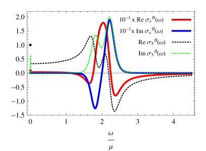
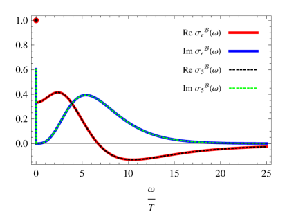
Figure 3: Frequency dependence of the vector and axial magnetic conductivities, $\sigma_{e}^{\cal B}$ and $\sigma_{5}^{\cal B}$, normalized to their zero frequency value, from a numerical evaluation of Eqs. (25) and (26). We consider $k=0$, $\mu=10\,\textrm{MeV}$, $\mu_{5}=1\,\textrm{MeV}$, $\tau=0.24$ (left figure) and $\tau=440$ (right figure). The vertical lines at $\omega=0$ in the imaginary parts are meant to remind one of the presence of the term $\sim\omega\delta(\omega)$. [Color online]

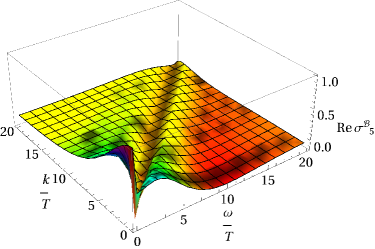
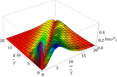
Figure 4: Frequency and momentum dependence of the axial magnetic conductivity $\sigma_{5}^{\cal B}(\omega,k)$ normalized to its zero frequency-momentum value, from a numerical evaluation of Eqs. (25) and (26). Left figure shows the real part, and right figure the imaginary part of the conductivity. We consider $\mu=10\,\textrm{MeV}$, $\mu_{5}=1\,\textrm{MeV}$, and temperature above the QCD phase transition $\tau=440$. The plots of the vector magnetic conductivity $\sigma_{v}^{\cal B}(\omega,k)$ are indistinguishable from these ones at this temperature. [Color online]

II.3 Thermodynamic variables

The pressure of the system can be computed from the correlator $G^{0z,0z}(k)=\langle T^{0z}(k)T^{0z}(-k)\rangle$, which at one loop reads

$$G^{0z,0z}(k_{0},k) = -\frac{1}{16\beta}\sum_{\tilde{\omega}}\int\frac{d^{3}q}{(2\pi)^{3}}\operatorname{tr\>}\Bigg{[}S(q)\gamma^{0}S(q+k)\gamma^{0}(2q^{z}+k^{z})^{2}+2S(q)\gamma^{0}S(q+k)\gamma^{z}(2i\tilde{\omega}+k^{0})(2q^{z}+k^{z})$$ (38)

$$+S(q)\gamma^{z}S(q+k)\gamma^{z}(2i\tilde{\omega}+k^{0})^{2}\Bigg{]}+\frac{3}{4}\left(\langle T^{zz}\rangle-\langle T^{00}\rangle\right)\,.$$

The last term is the contribution coming from the seagull diagram, see Manes and Valle (2013). The precise relation with the pressure reads

$$P=\lim_{\vec{k}\to 0}G^{0z,0z}(k_{0},k)\big{|}_{k_{0}=0}\,.$$ (39)

After an evaluation of Eq. (38), and considering the limits at zero frequency and momentum, the result for the pressure in the free theory reads

$$P=\frac{1}{6\pi^{2}}\int_{0}^{\infty}dq\,q^{3}\,f_{P}(q)=\frac{1}{12\pi^{2}}\left[\mu^{4}+6\mu^{2}\mu_{5}^{2}+\mu_{5}^{4}+2\pi^{2}T^{2}(\mu^{2}+\mu_{5}^{2})+\frac{7}{15}\pi^{4}T^{4}\right]\,,$$ (40)

where $f_{P}(q)=\sum_{s,t=\pm}n(E_{q}+t\mu_{s})$. This result corresponds to the pressure of an ideal gas of massless fermions of spin $1/2$ at finite temperature and chiral chemical potentials. By considering $\mu_{5}=0$ in the previous formula, we recover the standard result in the literature Le Bellac (1996). From this expression one may obtain the rest of thermodynamical quantities, in particular the energy density $\epsilon=3P$, entropy density

$$s=\frac{\partial P}{\partial T}=\frac{T}{45}\left(15(\mu^{2}+\mu_{5}^{2})+7\pi^{2}T^{2}\right)\,,$$ (41)

and the baryon and axial densities, respectively,

$$\rho_{e}=\frac{\partial P}{\partial\mu} = \frac{\mu}{3\pi^{2}}\left(\mu^{2}+3\mu_{5}^{2}+\pi^{2}T^{2}\right)\,,$$ (42)

$$\rho_{5}=\frac{\partial P}{\partial\mu_{5}} = \frac{\mu_{5}}{3\pi^{2}}\left(3\mu^{2}+\mu_{5}^{2}+\pi^{2}T^{2}\right)\,.$$ (43)

It is easy to check that previous relations fulfill

$$\epsilon+P=Ts+\mu n_{e}+\mu_{5}n_{5}\,.$$ (44)

The pressure can be obtained also from a direct computation of the thermodynamical potential of a free gas of fermions with chiral chemical potential, as it was done in Fukushima et al. (2008). Finally, notice that Eq. (40) can be expressed as a sum of right-handed and left-handed fermionic species contributing to the pressure, $P=P_{+}+P_{-}$, where

$$P_{\pm}=\frac{1}{24\pi^{2}}\left[\mu_{\pm}^{4}+2\pi^{2}T^{2}\mu_{\pm}^{2}+\frac{7}{15}\pi^{4}T^{4}\right]\,.$$ (45)

III Strongly coupled regime

To study the frequency dependence of a strongly coupled plasma we will use a holographic model similar to the one introduced in Landsteiner et al. (2011b). This model implements the gauge and mixed gauge-gravitational triangle anomalies. The difference of the present case with the model of Landsteiner et al. (2011b) is the inclusion of a conserved current which will be interpreted as the electric current beside the non conserved axial current. The presence of both currents in the model allows us to compute the frequency dependence of the chiral magnetic Yee (2009), separation and vortical effects.

The dual model consists on a five dimensional gravity theory with two gauge fields $U(1)_{V}\times U(1)_{A}$. The action writes

$$S = \frac{1}{16\pi G}\int d^{5}x\sqrt{-g}\left[R+12-\frac{1}{4}\left(F_{MN}F^{MN}+F^{(5)}_{MN}F^{(5)MN}\right)+\right.$$ (46)

$$\left.+\epsilon^{MNPQR}A^{(5)}_{M}\left(\frac{\kappa}{3}F^{(5)}_{NP}F^{(5)}_{QR}+\kappa F_{NP}F_{QR}+\lambda R^{A}\,_{BNP}R^{B}\,_{AQR}\right)\right]+S_{GH}+S_{CSK}\,,$$

$$S_{GH} = \frac{1}{8\pi G}\int_{\partial}d^{4}x\sqrt{-h}\,K\,,$$ (47)

$$S_{CSK} = -\frac{1}{2\pi G}\int_{\partial}d^{4}x\sqrt{-h}\,\lambda n_{M}\epsilon^{MNPQR}A^{(5)}_{N}K_{PL}D_{Q}K_{R}^{L}\,,$$ (48)

where $n_{A}$ is a normal vector to the $AdS$ boundary and $K_{MN}$ is the extrinsic curvature. In addition to this action it is necessary to include a boundary counterterm in order to make it finite.  This action is invariant under diffeomorphisms and vector gauge transformations, but it is not invariant under axial gauge transformations. The variation of the action under the latter shows results in the axial anomaly

$$\delta_{\xi_{5}}(S+S_{GH}+S_{CSK})=\frac{1}{16\pi G}\int_{\partial}d^{4}x\sqrt{-g}\,\xi_{5}\epsilon^{\mu\nu\rho\beta}\left(\frac{\kappa}{3}F^{(5)}_{\mu\nu}F^{(5)}_{\rho\beta}+\kappa F_{\mu\nu}F_{\rho\beta}+\lambda R^{\alpha}\,_{\delta\mu\nu}R^{\delta}\,_{\alpha\rho\beta}\right)\,.$$ (49)

This expression allows us to fix the value of the $\kappa$ and $\lambda$ parameters in terms of the anomalous coefficients of the field theory, so that

$$\frac{1}{16\pi G}\kappa=-\frac{1}{16\pi^{2}}\qquad,\qquad\frac{1}{16\pi G}\lambda=-\frac{1}{384\pi^{2}}.$$ (50)

This system admits a static charged black hole solution

$$ds^{2} = r^{2}\left(-f(r)dt^{2}+d\vec{x}^{2}\right)+\frac{dr^{2}}{r^{2}f(r)}\quad\,,\quad A=-\frac{\mu}{r^{2}}dt\quad\,,\quad A^{(5)}=-\frac{\mu_{5}}{r^{2}}dt\,,$$ (51)

where $f(r)=1-\frac{m}{r^{4}}+\frac{q^{2}}{r^{6}}$ is the blackening factor, while the mass and charge of the black hole are defined, respectively, as 

$$m = 1+q^{2}\quad\,,\quad q^{2}=\frac{\mu^{2}+\mu_{5}^{2}}{3}\,.$$ (52)

The Hawking temperature is given by $T=\frac{2m-3q^{2}}{2\pi}$. The extremal solution is obtained when $q=\sqrt{2}$. With these ingredients one can compute the pressure of the holographic model, and it reads 

$$P=\frac{m}{16\pi G}=\frac{1}{16\pi G}\left(\frac{\pi T}{2}\right)^{4}\left(\sqrt{1+\frac{2}{3}\frac{(\mu^{2}+\mu_{5}^{2})}{\pi^{2}T^{2}}}+1\right)^{3}\left(3\sqrt{1+\frac{2}{3}\frac{(\mu^{2}+\mu_{5}^{2})}{\pi^{2}T^{2}}}-1\right)\,.$$ (53)

As expected this result is different from the one obtained in the free gas of chiral fermions, cf. Eq. (40).

Our purpose is to compute two point retarded correlators in a linear response regime on top of this equilibrium background. To do so we need to introduce fluctuations of the gauge fields and metric components $A(t,y,r)=A_{(0)}(r)+\epsilon\,a(t,y,r)$, $A^{(5)}(t,y,r)=A_{(0)}^{(5)}(r)+\epsilon\,\tilde{a}(t,y,r)$ and $g_{MN}(t,y,r)=g^{(0)}_{MN}(r)+\epsilon\,h_{MN}(t,y,r)$. The nature of the correlators we want to compute tells us that it is enough to study only the shear sector. Allowing a $y$ dependence induces a breaking of rotational symmetry to the $SO(2)$ group around the axis defined by the $y$ coordinate. Therefore to study the shear sector it is enough to switch on the components

$$\Phi^{T}=(a_{x},\tilde{a}_{x},h_{t}^{x},h_{y}^{x},a_{z},\tilde{a}_{z},h_{t}^{z},h_{y}^{z})^{T}\,.$$ (54)

We will consider the gauge fixing $A_{r}=A^{(5)}_{r}=h_{rM}=0$. After introducing in the action this ansatz and taking variations with respect to the fluctuations we get the linearized equation of motions for the system,

$$0 = a_{i}^{\prime\prime}(u)+\frac{f^{\prime}}{f}a_{i}^{\prime}(u)+\frac{1}{4uf^{2}}\left(\omega^{2}-f{k}^{2}\right)a_{i}(u)-\frac{\mu}{f}h^{\prime i}_{t}(u)+\frac{4ik}{f}\kappa\epsilon_{ij}\left(\mu\tilde{a}_{j}(u)+\mu_{5}a_{j}(u)\right)\,,$$ (55)

$$0 = \tilde{a}_{i}^{\prime\prime}(u)+\frac{f^{\prime}}{f}\tilde{a}_{i}^{\prime}(u)+\frac{1}{4uf^{2}}\left(\omega^{2}-f{k}^{2}\right)\tilde{a}_{i}(u)-\frac{\mu_{5}}{f}h^{\prime i}_{t}(u)+\frac{4ik}{f}\epsilon_{ij}\left(\kappa(\mu a_{j}(u)+\mu_{5}a_{j}(u))+\lambda\frac{3\left(u^{3}\mu_{T}^{2}+2(f-1)\right)}{u}h^{\prime j}_{t}(u)\right)\,,$$

$$0 = h^{\prime\prime i}_{t}(u)-\frac{h^{\prime i}_{t}(u)}{u}-\frac{1}{4uf}\left(k^{2}h^{i}_{t}(u)+\omega kh^{i}_{y}\left(u\right)\right)-u(\mu_{5}\tilde{a}_{i}(u)+\mu a_{i}(u))^{\prime}+i\lambda uk\epsilon_{ij}\left[\frac{2k^{2}\mu_{5}}{f}h_{t}^{j}(u)-8\mu_{5}(uh^{\prime j}_{t}(u))^{\prime}\right.$$ (57)

$$\left.+\frac{2k\omega\mu_{5}}{f}h_{y}^{j}(u)-\frac{8}{3}\left((7u-3)\mu_{T}^{2}+8u\mu_{T}^{2}-9\right)\tilde{a}_{j}(u)-4u\left((5u-2)\mu_{T}^{2}-6\right)\tilde{a}^{\prime}_{j}(u)\right]\,,$$

$$0 = h^{\prime\prime i}_{y}(u)+\frac{\left(f/u\right)^{\prime}}{f/u}h^{\prime i}_{y}(u)+\frac{1}{4uf^{2}}\left(\omega^{2}h_{y}^{i}(u)+\omega kh_{t}^{i}(u)\right)+2uik\lambda\mu_{5}\epsilon_{ij}\left[-\frac{1}{f^{2}}(k\omega h_{t}^{j}(u)+\omega^{2}h_{z}^{j}(u))-4uh^{\prime\prime j}_{y}(u)\right.$$ (58)

$$\left.-4\left(3+\frac{u^{3}\mu_{T}^{2}-6}{3f}\right)h^{\prime j}_{y}(u)\right]\,,$$

and the constraints

$$0 = \omega h^{\prime i}_{t}+kfh^{\prime i}_{y}-u\omega(\mu_{5}\tilde{a}_{i}+\mu a_{i})-4ik\lambda\epsilon_{ij}\left(\omega\left(6(f-1)+3u^{3}\mu_{T}^{2}\right)\tilde{a}_{j}+2\mu_{5}u^{2}(\omega h^{\prime j}_{t}+kfh^{\prime j}_{y})\right)\,,$$ (59)

where we have redefined $\mu_{T}^{2}\equiv\mu^{2}+\mu_{5}^{2}$, $u=1/r^{2}$ and $i=x,z$. Notice that we also have Fourier transformed the fields.

As we are interested in computing retarded propagators we need to impose infalling boundary conditions at the horizon. This is the main boundary condition that must be satisfied. Since the system is second order we need a second boundary condition to specify a unique solution. This is done by demanding that the matrix of linearly independent solutions goes to the unit matrix at the boundary. These boundary conditions define the bulk-to-boundary propagator. In Son and Starinets (2002); Kaminski et al. (2010) a prescription to obtain two point functions in holography is discussed. The procedure is as follows: first we have to expand the renormalized action up to second order in the perturbative parameter $\epsilon$, and then Fourier transform it to get an expression of the form

$$\delta S^{(2)}=\int\frac{{\rm d}^{d}k}{(2\pi)^{d}}\{\Phi^{I}_{-k}{\cal A}_{IJ}\Phi^{\prime J}_{k}+\Phi^{I}_{-k}{\cal B}_{IJ}\Phi^{J}_{k}\}\Big{|}_{r\to\infty}\,.$$ (60)

On the other hand, we have to find a maximal set of linearly independent solutions satisfying ingoing boundary conditions and build the matrix $H^{I}_{J}(k,u)$ where each column consists of a solution of the linearly independent set. Finally the desired solution with the boundary sources switched on is

$$\Phi^{I}_{k}(u)=F^{I}\,_{J}(k,u)\,\varphi^{J}_{k}\,,$$ (61)

where $F=H(k,u)H^{-1}(k,0)$ and $\varphi^{J}_{k}$ are the sources of the dual field theory. From this we can read the retarded correlators which look like

$$G_{IJ}(k)=-2\lim_{u\to 0}\left({\cal A}_{IM}(F^{M}\,_{J}(k,u))^{\prime}+{\cal B}_{IJ}\right)\,.$$ (62)

After some tedious computation we can extract the matrices ${\cal A}$ and ${\cal B}$ for our system

$${\cal A}=\frac{1}{16\pi G}\mathrm{Diag}\left(f(u),f(u),-\frac{1}{u},\frac{f(u)}{u},f(u),f(u),-\frac{1}{u},\frac{f(u)}{u}\,\right)$$ (63)

and

$${\cal B}=\frac{1}{16\pi G}\left(\begin{array}[]{cc}B&0_{4\times 4}\\ 0_{4\times 4}&B\end{array}\right)\quad,\quad B=-\frac{1}{2}\left(\begin{array}[]{cccc}\left(k^{2}-\omega^{2}\right)\log u&0&0&0\\ 0&\left(k^{2}-\omega^{2}\right)\log u&-4\mu_{5}&0\\ 0&0&\frac{k^{2}}{u}+\frac{12}{u^{2}}&\frac{k\omega}{u}\\ 0&0&\frac{k\omega}{u}&\frac{\omega^{2}}{u}-\frac{12}{u^{2}}\end{array}\right)\,.$$ (64)

Now we have all the ingredients to compute the retarded Green functions and to use the Kubo formulae (2) and (3) to extract the anomaly induced transport coefficients. The zero frequency case can be done analytically by setting $\omega=0$ and looking for a linearized solution in the momentum $k$ (to see a detailed way of solving the system see Yee (2009); Gynther et al. (2011); Amado et al. (2011); Landsteiner et al. (2011b)). The conductivities in this case are

$$\sigma^{\cal B}_{A,(0)}=\frac{1}{2\pi^{2}}\left\{\begin{array}[]{l}\mu_{5}\\ \mu\\ \mu\mu_{5}\end{array}\right.\quad,\quad\sigma^{{\cal B}_{5}}_{A,(0)}=\frac{1}{2\pi^{2}}\left\{\begin{array}[]{l}\mu\\ \mu_{5}\\ \frac{\mu^{2}+\mu_{5}^{2}}{2}+\frac{\pi^{2}T^{2}}{6}\end{array}\right.\quad,\quad\sigma^{\cal V}_{A,(0)}=\frac{1}{2\pi^{2}}\left\{\begin{array}[]{l}\mu\mu_{5}\\ \frac{\mu^{2}+\mu_{5}^{2}}{2}+\frac{\pi^{2}T^{2}}{6}\\ \mu_{5}\left(\frac{\mu^{2}+\mu_{5}^{2}}{3}+\frac{\pi^{2}T^{2}}{3}\right)\end{array}\right.\,.$$ (74)

To study the frequency dependence we have to resort to numerics. The system of differential equations presents a singularity at $u=1$, so we have to implement a methodology to integrate the equations from this point to the boundary. As a first step we redefine the fields to ensure the infalling boundary condition

$$a^{i}(u) = (1-u)^{-iw}\,b^{i}(u)\,,$$ (75)

$$\tilde{a}^{i}(u) = (1-u)^{-iw}\,c^{i}(u)\,,$$ (76)

$$h^{i}_{t}(u) = (1-u)^{-iw+1}\,H^{i}_{t}(u)\,,$$ (77)

$$h^{i}_{y}(u) = (1-u)^{-iw}\,H^{i}_{y}(u)\,,$$ (78)

where $(w,P)=(\omega,k)/4\pi T$. Now the infalling condition is translated to a regularity condition on the fields $(b^{i},c^{i},H^{i}_{t},H^{i}_{y})$. Then we have to find eight linearly independent solutions to construct the matrix $F$, but the system is subject to two constraints reminding us that not all the fields are independent. Substituting these redefined fields into the constraints and evaluating them at the horizon, it is possible to find the relation

$$H_{y}^{i}(1) = \frac{3(i+w)}{P\left(\mu_{T}^{2}-6\right)}H_{t}^{i}(1)-\frac{27i\mu b^{i}(1)+i\mu_{5}\left(3+128P^{2}\lambda^{2}\left(\mu_{T}^{2}-6\right)^{2}\left(\mu_{T}^{2}-2\right)\right)c^{i}(1)}{P\left(\mu_{T}^{2}-6\right)\left(256P^{2}\lambda^{2}\mu_{5}^{2}\left(\mu_{T}^{2}-6\right)^{2}-9\right)}$$ (79)

$$-\lambda\epsilon_{ij}\frac{16\mu\mu_{5}b^{j}(1)+72\left(\mu_{T}^{2}-6\right)^{2}c^{j}(1)}{256P^{2}\lambda^{2}\mu_{5}^{2}\left(\mu_{T}^{2}-6\right)^{2}-9}.$$

This formula makes clear that we only have freedom to fix the six values $(H_{t}^{i}(1),b^{i}(1),c^{i}(1))$, while the remaining two are given by pure gauge solutions arising from gauge transformations of the trivial solution. We choose them to be

$$\Phi(1)=\begin{array}[]{cccccccc}\left(\begin{array}[]{c}1\\ 0\\ 0\\ H_{y}^{x}(1)\\ 0\\ 0\\ 0\\ H_{y}^{z}(1)\end{array}\right),&\left(\begin{array}[]{c}0\\ 1\\ 0\\ H_{y}^{x}(1)\\ 0\\ 0\\ 0\\ H_{y}^{z}(1)\end{array}\right),&\left(\begin{array}[]{c}0\\ 0\\ 1\\ H_{y}^{x}(1)\\ 0\\ 0\\ 0\\ H_{y}^{z}(1)\end{array}\right),&\left(\begin{array}[]{c}0\\ 0\\ w\\ -p\\ 0\\ 0\\ 0\\ 0\end{array}\right)\,,&\left(\begin{array}[]{c}0\\ 0\\ 0\\ H_{y}^{x}(1)\\ 1\\ 0\\ 0\\ H_{y}^{z}(1)\end{array}\right),&\left(\begin{array}[]{c}0\\ 0\\ 0\\ H_{y}^{x}(1)\\ 0\\ 1\\ 0\\ H_{y}^{z}(1)\end{array}\right),&\left(\begin{array}[]{c}0\\ 0\\ 0\\ H_{y}^{x}(1)\\ 0\\ 0\\ 1\\ H_{y}^{z}(1)\end{array}\right),&\left(\begin{array}[]{c}0\\ 0\\ 0\\ 0\\ 0\\ 0\\ w\\ -p\end{array}\right)\,.\end{array}$$ (145)

With these first eight vectors we can find numerically the linearly independent solutions. The matrix $H$ is built up as $H^{I}_{J}(u)=(\Phi^{I}(u))_{J}$. For the numerical computation we use the values $\kappa=1$ and $\lambda=1/24$ since we know from Eq. (50) the ratio $\lambda/\kappa=1/24$.

As the Kubo formulae demand to take the limit $k\to 0$ we fixed the infrared cutoff momentum $P_{c}=1/1000$. We study first the case of interest for heavy ion collisions, that corresponds to the high temperature situation. In particular if we assume the vector chemical potential is of order $10\,$MeV and a temperature around the QCD critical temperature $T_{c}=160\,$MeV, that fixes $\tau=95$. For temperatures of order $700\,$MeV we get $\tau=440$. In what follows we will analyze the theory for these two particular temperatures.

Figures 5 and 6 show the behavior of the chiral vortical conductivities. Figure 5 is quite similar to the weakly coupled behavior. Once the frequency moves away from zero, the conductivity in the strongly coupled regime drops 6 orders of magnitude and shows a damped oscillation. In the free fermion case we have seen that the vortical conductivities are defined as piecewise functions of the frequency, when the source is a homogeneous function of the space coordinates. However in the present case we are obtaining fast decaying functions of the frequency but with a non vanishing width. Therefore to study whether the strongly coupled coefficients have the decay smoothed by the strong interaction, or whether we see a width as a consequence of the small but non vanishing momentum used for the numerics, we compute the conductivities evaluating them at three infrared cut-off momenta for temperature $\tau=95$ and chemical potentials $\mu_{5}/\mu=0.008$. Then in figure 6 we plot all the fast decaying conductivities as a function of $4\pi T\omega/k_{c}^{2}$ for the dimensionless momentum values $P_{c}=1/10,1/100,1/1000$. Analyzing the plot we realize that the approximate position of either the peaks in the imaginary part or the width in the real part is of order $\omega\sim k_{c}^{2}/(4\pi T)$. Then we can infer that the conductivities for a homogeneous source vanish at $\omega\neq 0$, and they are discontinuous functions at $\omega=0$, coinciding exactly with the weakly coupled conductivities. Notice that the constant $1/(4\pi T)$ is the shear diffusion constant, this number suggests that this small frequency and momentum behavior are governed by hydrodynamics This point will be addressed in section IV.

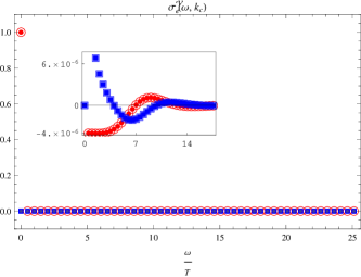
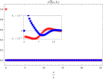
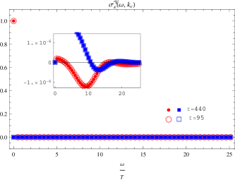
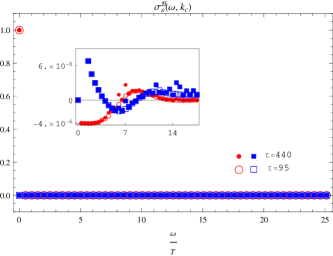
Figure 5: Frequency dependence of the chiral vortical conductivities and chiral magnetic energy conductivity for finite chemical potentials and temperature around the QCD critical value ($\tau=95$, $\mu_{5}/\mu=0.008$) and temperature above the phase transition ($\tau=440$, $\mu_{5}/\mu=0.03$). Red circles represent the real part of the conductivities and blue squares the imaginary part. [Color online]

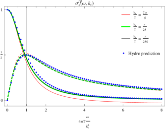
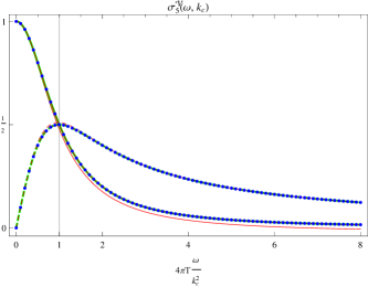
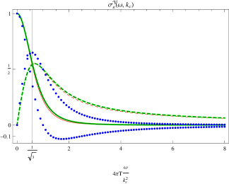
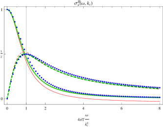
Figure 6: Study of the width of the vortical conductivities with the infrared momentum cut-off used for the numerics. Solid and dashed lines show the real and imaginary parts, respectively. Red lines show $P_{c}=1/10$, green $P_{c}=1/100$ and black $P_{c}=1/1000$. The parameters are ($\tau=95$, $\mu_{5}/\mu=0.008$). Dots are the hydrodynamical fit (see section IV) and the vertical lines represent the positions of the maxima predicted by hydrodynamics. Notice that the regime in frequencies in this figure is much smaller than the one in figure 5. [Color online]

The frequency dependence of the magnetic conductivities in a holographic model was studied first in Yee (2009) but the mixed gauge-gravitational anomaly was not included. For that reason and for completeness we also show in figure 7 these conductivities. Notice that at the temperatures considered the conductivities are not affected by a change in temperature (when they are plotted as a function of $\omega/T$) and the position of the peak of the imaginary part is at $\omega\sim 5T$ as in the weakly coupled case for high temperatures, in agreement with the result for $\sigma^{\cal B}_{e}$ in Yee (2009). The only difference in the frequency dependence introduced by the mixed anomaly with respect to the former reference is the small jump in the conductivity at small frequency (see green curves in Fig. 7). A difference with Sec. II is also remarkable: the frequency dependence of $\sigma^{{\cal B}_{5}}_{5}(\omega)$ is slightly different from $\sigma^{\cal B}_{e}(\omega)$. There is another qualitative similarity with the model of Sec. II: for both theories the frequency in which the magnetic conductivities vanish is $\omega\sim 15T$. The system becomes “insulator” if the frequency of the magnetic field is higher than this specific value.

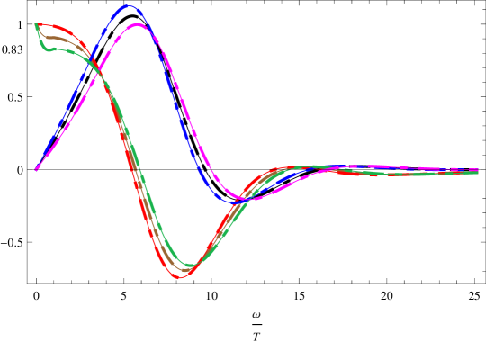
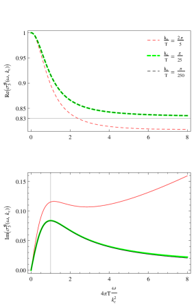
Figure 7: Frequency dependence of the chiral magnetic conductivities for high temperatures. Thick dashed lines correspond to $\tau=440$ and continuous lines to $\tau=95$. Red and blue are real and imaginary parts of $\sigma_{e}^{\cal B}$ respectively, brown and black lines real and imaginary parts of $\sigma_{5}^{\cal B}$, green and magenta lines are real and imaginary part of $\sigma_{5}^{{\cal B}_{5}}$. [Color online]

Then we solved the system for very low temperatures to study the zero temperature behavior. In figure 8 we can see in the magnetic conductivities a jump at zero frequency as in the weakly coupled case, plus a resonance at $\omega\neq 0$. Another similar feature with weak coupling is the plateau at small frequencies in the chiral separation effect. To finish we study the frequency and momentum dependence of the conductivities. The strongly coupled regime does not show a qualitative difference with respect to the weakly coupled case in the regime of interest. We show in figure 9 the conductivities, $\mathop{\rm Re}[\sigma_{5}^{\cal V}(\omega,k)]$ and $\mathop{\rm Re}[\sigma_{5}^{\cal B}(\omega,k)]$. The vortical conductivities in both models, the weakly coupled and strongly coupled one, require inhomogeneities in the vortex in order for a current being produced. The phenomenological implications for the chiral vortical effect in the quark gluon plasma will be discussed in the section VI.

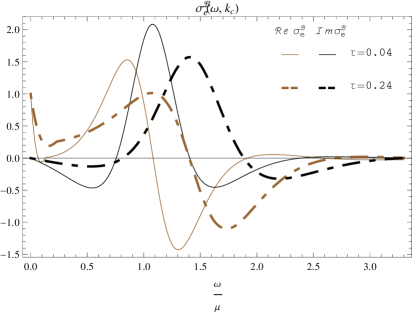
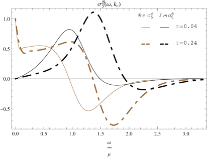
Figure 8: Frequency dependence of the chiral magnetic conductivities for temperatures close to zero, ($\tau=0.04$, $\mu_{5}/\mu=7\times 10^{-5}$) and ($\tau=0.24$, $\mu_{5}/\mu=0.7$).

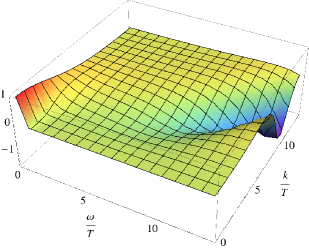
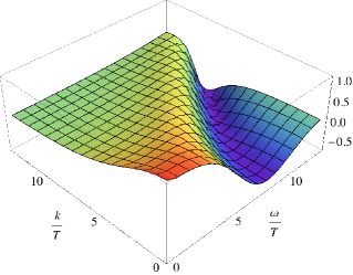
Figure 9: Left plot shows the real part of $\sigma^{\cal V}_{5}(\omega,k)$ and the right plot is the real part of $\sigma^{\cal B}_{5}(\omega,k)$. [Color online]

IV Two point functions in hydrodynamics

To have a better understanding of the results obtained in the previous sections, we will compute the form predicted by hydrodynamics of the two point functions of interest. To do so we start with the first order constitutive relations for a fluid with an anomalous $U(1)$.  

$$T^{\mu\nu} = (\epsilon+P)u^{\mu}u^{\nu}+Pg^{\mu\nu}-\eta\sigma^{\mu\nu}+\sigma_{\epsilon}^{\cal B}(B^{\mu}u^{\nu}+B^{\nu}u^{\mu})+\sigma_{\epsilon}^{\cal V}(\omega^{\mu}u^{\nu}+\omega^{\nu}u^{\mu})\,,$$

$$J^{\mu} = \rho u^{\mu}+\sigma^{\cal B}B^{\mu}+\sigma^{\cal V}\omega^{\mu}\,.$$ (147)

As the anomalous transport is also present in equilibrium, we also assume electro-chemical equilibrium. This assumption allows us to remove the thermoelectric terms. Apart from the constitutive relations we need the energy conservation

$$\nabla_{\mu}T^{\mu\nu}=F^{\nu\mu}J_{\mu}\,,$$ (148)

and solve for the velocities which are the unknown variables in the system. To do so, we will consider small fluctuations for the background fields $(h,A)$, $g_{\mu\nu}=\eta_{\mu\nu}+h_{\mu\nu}(t,x)$ and $A_{\mu}(t,x)$ and we will expand the expressions up to first order in them. These fluctuations will take the fluid away from equilibrium, so that the new fluid velocity can be written as $u^{\mu}=(1,v^{i}(t,x))$, where $v^{i}$ will also be small. In particular to study the shear sector it is necessary to switch on only $h_{ty}(t,x),$ $h_{tz}(t,x),$ $h_{xy}(t,x),$ $h_{xz}(t,x)$ and $A_{y}(t,x),$ $A_{z}(t,x)$. After plugging all these ingredients in the constitutive relations and Fourier transforming them, we end up with

$$T^{ti} = (\epsilon+P)v_{i}+Ph_{ti}-ik\epsilon_{ij}\sigma_{\epsilon}^{\cal V}(v_{j}+h_{tj})-ik\epsilon_{ij}\sigma_{\epsilon}^{\cal B}A_{j}\,,$$ (149)

$$T^{xi} = -Ph_{xi}+i\eta(\omega h_{xi}-kv_{i})\,,$$ (150)

$$J^{i} = \rho v_{i}-ik\epsilon_{ij}\sigma^{\cal V}(v_{j}+h_{tj})-ik\epsilon_{ij}\sigma^{\cal B}A_{j}\,,$$ (151)

where $i,j=y,z$ and $\epsilon_{ij}$ is the antisymmetric symbol. The conservation law is

$$-\epsilon_{ij}\sigma_{\epsilon}^{\cal B}\omega kA_{j}+(-i\omega(\epsilon+P)+\eta k^{2})v_{i}-i\omega(P+\epsilon)h_{ti}-\epsilon_{ij}\sigma_{\epsilon}^{\cal V}\omega k(h_{tj}+v_{j})-\eta\omega kh_{xi}-i\omega A_{i}\rho=0\,.$$ (152)

Using these equations one can solve for the velocities. Next we plug the solutions into the constitutive relations and use linear response to relate these expressions with the two point functions of interest. Using the scaling limit $(\omega,k)\rightarrow(z^{2}\omega,zk)$ for $z\ll 1$ as appropriate for isolating the diffusion pole in the shear channel, we arrive at the correlators

$$\langle T^{ti}T^{tj}\rangle = -i\epsilon_{ij}k\sigma_{\epsilon}^{\cal V}\frac{-D^{2}k^{4}}{(\omega+iDk^{2})^{2}}\,,$$ (153)

$$\langle T^{ti}J^{j}\rangle = -i\epsilon_{ij}k\left(\sigma_{\epsilon}^{\cal B}-\frac{\rho\sigma_{\epsilon}^{\cal V}}{\epsilon+P}\frac{\omega}{\omega+iDk^{2}}\right)\frac{iDk^{2}}{\omega+iDk^{2}}\,,$$ (154)

$$\langle J^{i}T^{tj}\rangle = -i\epsilon_{ij}k\left(\sigma^{\cal V}-\frac{\rho\sigma_{\epsilon}^{\cal V}}{\epsilon+P}\frac{\omega}{\omega+iDk^{2}}\right)\frac{iDk^{2}}{\omega+iDk^{2}}\,,$$ (155)

$$\langle J^{i}J^{j}\rangle = -i\epsilon_{ij}k\left(\sigma^{\cal B}-\frac{\rho}{\epsilon+P}\left[2\sigma^{\cal V}-\frac{\rho\sigma_{\epsilon}^{\cal V}}{\epsilon+P}\frac{\omega}{\omega+iDk^{2}}\right]\frac{\omega}{\omega+iDk^{2}}\right)\,,$$ (156)

where the shear diffusion constant is defined as $D=\eta/(\epsilon+P)$. The mixed correlators $\langle JT\rangle$ and $\langle TJ\rangle$ are exactly the same because $\sigma_{\epsilon}^{\cal B}=\sigma^{\cal V}$. We also note that all three conductivities associated with correlators containing the energy current $T^{ti}$ vanish in the limit $k\rightarrow 0$ at finite frequency $\omega$. This is just the same behavior we have already observed in our explicit weak and strong coupling calculations. From these expressions we can compute the position of the maxima in the real part of the correlators by just solving the equations

$$\frac{d}{d\omega}\mathop{\rm Re}\langle T^{ti}T^{tj}\rangle\left|{}_{\omega_{M}}\right. = 0\,,$$ (157)

$$\frac{d}{d\omega}\mathop{\rm Re}\langle T^{ti}J^{j}\rangle\left|{}_{\omega_{M}}\right. = 0\,,$$ (158)

$$\frac{d}{d\omega}\mathop{\rm Re}\langle J^{i}J^{j}\rangle\left|{}_{\omega_{M}}\right. = 0\,.$$ (159)

The real parts are related to the imaginary parts of the conductivities, cf. Eqs. (2) and (3). These equations have the solutions

$$\omega_{M} = \pm\frac{1}{\sqrt{3}}Dk^{2}\qquad\textrm{for}\qquad\langle T^{ti}T^{tj}\rangle\,,$$ (160)

$$\omega_{M} \simeq \pm Dk^{2}\qquad\quad\;\;\,\textrm{for}\qquad\langle T^{ti}J^{j}\rangle\,,\quad\langle J^{i}T^{tj}\rangle\quad\textrm{and}\quad\langle J^{i}J^{j}\rangle\,.$$ (161)

The results derived in this section for the vortical conductivities are plotted in figure 6. The holographic results shown in figure 6 have the same behavior as the hydrodynamic computation. In particular, the position of the maxima in the imaginary part of the conductivities agrees quite well with Eqs. (160) and (161). Actually even in the magnetic conductivities we can see at small enough frequency the effect of the presence of the diffusion mode in consistency with Eqs. (156) and (161), see figure 7.

V Ward Identities

In this section we will show that the vanishing of the chiral vortical conductivities for non zero frequency follows from energy-momentum conservation. We therefore study what we can learn from the Ward identities for diffeomorphisms. In particular we want to study the correlators that correspond to the Kubo formulas for the chiral vortical conductivities and the chiral magnetic conductivity for the energy current.

We start with the form of the transformations on metric and gauge field

$$\delta g_{\mu\nu} =-\nabla_{\mu}\epsilon_{\nu}-\nabla_{\nu}\epsilon_{\mu}\,$$ (162)

$$\delta A_{\mu} =-\partial_{\mu}(\epsilon^{\nu}A_{\nu})-\epsilon^{\nu}F_{\mu\nu}\,,$$ (163)

under an infinitesimal diffeomorphism $x^{\mu}\rightarrow x^{\mu}+\epsilon^{\mu}$. We assume that the Green functions are obtained from an effective action $W[g_{\mu\nu},A_{\mu}]$ such that under the diffeomorphism

$$\delta W=\int d^{4}x\left(\frac{\delta W}{\delta g_{\mu\nu}(x)}\delta g_{\mu\nu}(x)+\frac{\delta W}{\delta A_{\mu}(x)}\delta A_{\mu}(x)\right)=0\,.$$ (164)

We have assumed that all mixed gauge-gravitational anomalies are shifted into the axial current via a suitable renormalization scheme. Since $\epsilon^{\mu}(x)$ is an arbitrary vector we can derive the local diffeomorphism Ward identity

$$\nabla_{\mu}\left(\frac{2}{\sqrt{-g}}\frac{\delta W}{\delta g_{\mu\nu}(x)}\right)+\nabla_{\mu}\left(\frac{1}{\sqrt{-g}}\frac{\delta W}{\delta A_{\mu}(x)}\right)A^{\nu}(x)+\frac{1}{\sqrt{-g}}\frac{\delta W}{\delta A_{\mu}(x)}F_{\mu}\,^{\nu}(x)=0\,.$$ (165)

We note that the energy-momentum tensor and the current are

$$T^{\mu\nu} =\frac{2}{\sqrt{-g}}\frac{\delta W}{\delta g_{\mu\nu}(x)}\,$$ (166)

$$J^{\mu}(x) =\frac{1}{\sqrt{-g}}\frac{\delta W}{\delta A_{\mu}(x)}\,.$$ (167)

In the flat space limit we can write $T^{\mu\nu}=2\delta W/\delta h_{\mu\nu}$ for $g_{\mu\nu}=\eta_{\mu\nu}+h_{\mu\nu}$. We can obtain the wanted Ward identities by differentiating Eq. (165) with respect to the sources $g_{\mu\nu}(y)$ and $A_{\mu}(y)$. We have assumed here that the metric has Euclidean signature. To obtain expressions for retarded Green’s functions in the Minkowski signature we need to analytically continue the metric and the frequency. The analytic continuation in the metric implies that all Euclidean timelike indices on operators obey $T^{\tau\mu}\rightarrow iT^{0\mu}$. The Euclidean frequency is analytically continued in the standard way $i\omega_{n}=\omega+i\epsilon$.

V.0.1 Chiral vortical conductivity in energy current

Let us start with another differentiation with respect to $g_{\mu\nu}(y)$. Since we only want Ward identities in the absence of external sources we set $A_{\mu}=0$ from the outset. We observe

$$\Gamma^{\mu}_{\mu\rho} =\frac{1}{2}g^{\mu\lambda}\left(\partial_{\mu}g_{\lambda\rho}+\partial_{\rho}g_{\lambda\mu}-\partial_{\lambda}g_{\mu\rho}\right)=\frac{1}{2}g^{\mu\lambda}\partial_{\rho}g_{\mu\lambda}\,$$ (168)

$$\partial_{\rho}\frac{1}{\sqrt{-g}} =-\frac{1}{2}g^{\mu\lambda}\partial_{\rho}g_{\mu\lambda}\,.$$ (169)

This leads to the simplified identity

$$\partial_{\mu}\left(\frac{\delta W}{\delta g_{\mu\nu}(x)}\right)+\Gamma^{\nu}_{\mu\rho}\frac{\delta W}{\delta g_{\mu\rho}(x)}=0\,.$$ (170)

Since we need to differentiate only once with respect to the external metric it is sufficient to use the linearized background metric $g_{\mu\nu}=\eta_{\mu\nu}+h_{\mu\nu}$ in order to compute the Christoffel symbol

$$\Gamma^{\mu}_{\nu\lambda}=\frac{1}{2}\eta^{\mu\sigma}\left(\partial_{\nu}h_{\sigma\lambda}+\partial_{\lambda}h_{\sigma\nu}-\partial_{\sigma}h_{\nu\lambda}\right)\,.$$ (171)

Then we get the Ward identity

$$\partial_{\mu}^{x}\Pi^{\kappa\lambda,\mu\nu}(y,x)+\eta^{\nu\kappa}\partial_{\mu}^{x}\delta(x-y)T^{\mu\lambda}(x)+\eta^{\nu\lambda}\partial_{\mu}^{x}\delta(x-y)T^{\mu\kappa}(x)-\eta^{\mu\nu}\partial_{\mu}^{x}\delta(x-y)T^{\kappa\lambda}(x)=0\,,$$ (172)

where we also used the definition

$$\Pi^{\lambda\kappa,\mu\nu}(y,x)=4\left.\frac{\delta^{2}W}{\delta g_{\lambda\kappa}(y)\delta g_{\mu\nu}(x)}\right|_{g_{\mu\nu}=\eta_{\mu\nu}}$$ (173)

This definition includes the seagull term, so that

$$\Pi^{\lambda\kappa,\mu\nu}(y,x)=\left\langle T^{\lambda\kappa}(y)T^{\mu\nu}(x)\right\rangle+\mathrm{seagull}\,.$$ (174)

We assume translational invariance such that $\langle T^{\mu\nu}(x)\rangle=\langle T^{\mu\nu}(0)\rangle=T_{0}^{\mu\nu}$. The Fourier transformed Ward identity is now

$$k_{\mu}\left(\tilde{\Pi}^{\lambda\kappa,\mu\nu}(k)+\eta^{\nu\lambda}T_{0}^{\mu\kappa}+\eta^{\kappa\nu}T_{0}^{\mu\lambda}-\eta^{\mu\nu}T_{0}^{\kappa\lambda}\right)=0\,.$$ (175)

To be able to say something about the chiral vortical conductivity in the energy current we evaluate this Ward identity in the polarization $k_{\mu}=(k_{0},0,0,k_{z})$, $\kappa=x$, $\nu=y$ and $\lambda=\tau$ with $\tau$ being Euclidean time. In any case, none of the contact terms in (175) contributes for our choice of polarization.

$$k_{\tau}\tilde{\Pi}^{\tau x,\tau y}+k_{z}\tilde{\Pi}^{\tau x,zy}=0\,.$$ (176)

Now we write $k_{\tau}=\omega_{n}$ and also analytically continue the $\tau$ indices in the correlators and arrive at

$$-\omega_{n}\tilde{\Pi}^{0x,0y}+ik_{z}\tilde{\Pi}^{0x,zy}=0\,.$$ (177)

Finally we get the Ward identity for the retarded Green’s function by setting $i\omega_{n}=\omega+i\epsilon$ such that

$$i(\omega+i\epsilon)\frac{\tilde{\Pi}^{0x,0y}(i\omega_{n}=\omega+i\epsilon,k_{z})}{ik_{z}}=-\tilde{\Pi}^{0x,zy}(i\omega_{n}=\omega+i\epsilon,k_{z})\,.$$ (178)

Now we take the limit $k_{z}\rightarrow 0$. On the left hand side we just obtain the frequency dependent chiral vortical conductivity multiplied with the frequency. The correlator on the right hand side is evaluated at zero momentum. This correlator can be further constrained via rotational symmetry. Under a rotation by $\pi/2$ along the $x$-axis $\tilde{\Pi}^{0x,zy}(\omega,\vec{k}=0)$ transforms as a symmetric tensor and this implies $\tilde{\Pi}^{0x,zy}(\omega,0)=-\tilde{\Pi}^{0x,yz}(\omega,0)$. Since the correlator is symmetric in the $y,z$ indices this implies that it must vanish $\Pi^{0x,yz}(\omega,0)=0$. Therefore we find for the chiral vortical conductivity

$$\omega\,\sigma^{\cal V}_{\epsilon}(\omega)=0\,.$$ (179)

V.1 Chiral vortical conductivity in charge current

Again we start from the Ward identity (165). Now we want to differentiate with respect to the external gauge field. Therefore we can directly set $g_{\mu\nu}=\eta_{\mu\nu}$ in (165). Differentiating with respect to $A_{\lambda}(y)$ and then setting $A_{\mu}=0$ and doing the Fourier transform as before gives

$$k_{\mu}\left(\tilde{G}^{\lambda,\mu\nu}(k)+J^{\mu}_{0}\eta^{\lambda\nu}-J^{\lambda}_{0}\eta^{\mu\nu}\right)=0\,,$$ (180)

where

$$(2\pi)^{4}G^{\lambda,\mu\nu}(k)=\langle J^{\lambda}(k)T^{\mu\nu}(-k)\rangle$$ (181)

Going through the same steps as before we arrive at

$$i(\omega+i\epsilon)\left.\frac{\tilde{G}^{x,0y}(i\omega_{n}=\omega+i\epsilon,k_{z})}{ik_{z}}\right|_{k_{z}\rightarrow 0}=\tilde{G}^{x,zy}(i\omega_{n}=\omega+i\epsilon,\vec{k}=0)\,.$$ (182)

Invariance under rotations around the $x$ axis implies as before $\tilde{G}^{x,zy}(\omega,0)=0$ and therefore

$$\omega\,\sigma^{\cal V}(\omega)=0\,.$$ (183)

V.2 Chiral magnetic conductivity in energy current

Now we need to get the correlators in reversed order. In the Euclidean theory this is easy, since the functional derivatives with respect to the metric and the gauge field commute. Therefore we also have the Ward identity

$$\partial^{x}_{\mu}\langle T^{\mu y}(x)J^{x}(y)\rangle=0\,,$$ (184)

and this leads then to

$$i\omega\frac{\langle T^{0y}(k)J^{x}(-k)\rangle}{ik_{z}}=\langle T^{zy}(k)J^{x}(-k)\rangle\,.$$ (185)

Taking the limit $k_{z}\rightarrow 0$ and using the resulting invariance under rotation along the $x$ axis gives

$$\omega\,\sigma^{\cal B}_{\epsilon}(\omega)=0\,.$$ (186)

The relations (186), (183) and (179) indeed imply that the chiral vortical conductivities and the chiral magnetic conductivity in the energy current vanish for non-zero frequency as we have indeed found in our explicit calculations at weak and strong coupling.

VI Discussion

The main result in our study is the behavior of the chiral vortical conductivities as a function of the frequency. The weak and strong coupling analysis produce the same result for the conductivities associated with a homogeneous and time dependent vortex, and it reads

$$\sigma^{\cal V}_{A}(\omega)=\sigma_{A,(0)}^{\cal V}\left(\delta_{\omega,0}+i\pi\omega\delta(\omega)\right)\,,\qquad A=e,5,\epsilon\,.$$ (187)

In section V we understood that this behavior in the vortical conductivities is a requirement of energy-momentum conservation. That is the reason why the conductivities for free fermions and for the strongly coupled model show the same non-analyticity. Therefore, for any theory with a conserved stress energy tensor the vortical conductivities at zero momentum must be of the form of Eq. (187). However, the magnetic conductivities in the currents are not subject to this constraint because they are computed via two point functions of charged currents. Hence the frequency dependence of the magnetic conductivities will be model dependent. The non-commutativity of the limits $\omega\rightarrow 0$ and $k\rightarrow 0$ in the magnetic conductivities (of the currents) is still induced by the mixing with the shear channel but it is of quite different nature and does not lead to the behavior (187).

To better understand the meaning of Eq. (187) and the response pattern in real time we consider a test body initially at rest which we start to rotate with constant angular velocity $\Omega_{k}$ at time $t=0$ such that the driving force is $\Omega_{k}\Theta(t)$ for a selected wave-number $k$. We use the hydrodynamic approximation (155) for the response function. The real time response in the current is then given by the Fourier transform

$$J(t) =\Omega_{k}\int\frac{d\omega}{2\pi}{\rm e}^{-i\omega t}\left(\sigma_{0}^{\cal V}\frac{iDk^{2}}{\omega+iDk^{2}}-\frac{\rho\sigma^{\cal V}_{\epsilon}}{\epsilon+P}\frac{\omega iDk^{2}}{(\omega+iDk^{2})^{2}}\right)\frac{i}{\omega+i\epsilon}=\theta(t)\Omega_{k}\left[\sigma_{0}^{\cal V}(1-e^{-Dk^{2}t})-\frac{\rho\sigma^{\cal V}_{\epsilon}}{\epsilon+P}Dk^{2}te^{-Dk^{2}t}\right]\,.$$ (188)

The non-analytic behavior is now exhibited by the non-commutativity of the limits $t\rightarrow\infty$ and $k\rightarrow 0$ (for simplicity we assume $\Omega_{k}$ to be finite in the limit $k\rightarrow 0$). If we first take $t$ to infinity we end up with the equilibrium response determined by the value of $\sigma_{0}^{\cal V}$. On the other hand, if we take $k$ to zero first, we find that there is actually no response at any finite value of $t$. In most physical situations the wave number is limited effectively by the inverse of the linear size of the system, which provides an infrared cutoff. Of course, the lifetime of the system should be long enough for the exponential in (188) to decay. It is a tempting exercise to insert some typical numbers for the strongly coupled quark gluon plasma. We note that the momentum diffusion constant is given by $D=\frac{\eta}{\varepsilon+p}\approx\frac{1}{4\pi T}$ where we assumed the shear viscosity to obey $s=4\pi\eta$ and neglected the chemical potentials . Using as cutoff the typical size of a fireball created in heavy ion collisions $L\approx 10\,\mathrm{fm}$ and defining the decay time as $t_{c}=1/Dk^{2}$ we find therefore $t_{c}\approx 4\pi TL^{2}$. Putting in the units $T=350\,\mathrm{MeV}$, $L=10\,\mathrm{fm}$ and the conversion factor $\hbar c=197\,\mathrm{MeV\,fm}$ we obtain $t_{c}\sim 2200\,\mathrm{fm/c}$. Since the lifetime of the quark gluon plasma is limited to $\tau\sim 10\mathrm{fm/c}$ this means that there is essentially no response of such a droplet of strongly coupled quark gluon plasma to a forced rotation on such a short time scale compared with the size of the system ($\tau\ll TL^{2}$). This very crude estimate should of course not be taken too seriously. The physical situation in a heavy ion collision is much more complicated and does not correspond to rotation driven by an external force to which our response formulas apply. To really understand better the role the chiral vortical effect plays in heavy ion collisions one needs to set up an initial value problem and solve the hydrodynamic evolution equations. This is a much more complicated problem and far beyond the scope of this article. Nevertheless we think that our considerations raise the question of how effective the chiral vortical effect might be in systems of finite lifetime even if they are large enough to be well modeled via hydrodynamics. Hopefully these questions can be addressed via numerical methods in the near future.

VII Acknowledgments

We would like to thank Juan L. Mañes for useful clarifications on the seagull term, Ho-Ung Yee for discussions and especially Dam T. Son for a very useful discussion on the interpretation of our results. This work has been supported in part by Plan Nacional de Altas Energías (FPA2011-25948 and FPA2012-32828), Spanish MICINN Consolider-Ingenio 2010 Program CPAN (CSD2007-00042), Comunidad de Madrid HEP-HACOS S2009/ESP-1473. Also by European Union’s Seventh Framework Programme under grant agreements (FP7-REGPOT-2012-2013-1) no 316165, PIF-GA-2011-300984, the EU program “Thales” and “HERAKLEITOS II” ESF/NSRF 2007-2013 and was also co-financed by the European Union (European Social Fund, ESF) and Greek national funds through the Operational Program “Education and Lifelong Learning” of the National Strategic Reference Framework (NSRF) under “Funding of proposals that have received a positive evaluation in the 3rd and 4th Call of ERC Grant Schemes”. The authors acknowledge also the support of the Spanish MINECO’s “Centro de Excelencia Severo Ochoa” Programme under grants SEV-2012-0234 and SEV-2012-0249. E.M. acknowledges the warm hospitality and partial support from the Instituto de Física Teórica IFT-UAM/CSIC, where parts of this work were carried out. The research of E.M. is supported by the Juan de la Cierva Program of the Spanish MINECO.

*

Appendix A Sum over Matsubara frequencies

In this Appendix we would like to discuss a subtle point on the definition of the currents and the chemical potentials that appear in the calculations. In particular we want to point out that there are two, usually equivalent ways of calculating the sum over Matsubara frequencies and to analytically continue to Lorentzian signature.

The textbook way of introducing the chemical potential is as follows. Consider a system of fermions with creation and annihilation operators $c^{\dagger}_{k}$ and $c_{k}$. At zero temperature and finite density all states up to a maximum energy are occupied. For free fermions the Fermi energy is just the chemical potential $\mu$. Let us label this state by $|\mu\rangle$. The creation and annihilation operators corresponding to momenta $k$ such that $\omega(k)<\mu$ acting on the state $|\mu\rangle$ change roles because of the Pauli principle. Within that range of energies we have

$$c_{k}|\mu\rangle=|\mu-1\rangle\,,$$ (189)

$$c^{\dagger}_{k}|\mu\rangle=0\,.$$ (190)

The state $|\mu-1\rangle$ is the state in which the fermionic quantum of momentum $k$ is missing (a hole state). Therefore in this momentum range $c_{k}$ acts as creation operator (of holes) and $c^{\dagger}_{k}$ as annihilation operator. This motivates us to introduce a new Hamiltonian that counts energy not with respect to the normal ordered vacuum but with respect to the finite density state $|\mu\rangle$. The Hamiltonian measuring energy with respect to the normal ordered vacuum is

$$H_{0}=\sum_{k}\omega(k)c^{\dagger}_{k}c_{k}$$ (191)

whereas the Hamiltonian measuring energies with respect to the Fermi energy are $\hat{H}=\sum_{k}[\omega(k)-\mu]c^{\dagger}_{k}c_{k}$ Therefore it is natural to define a new Hamiltonian

$$\hat{H}=H_{0}-\mu Q$$ (192)

where $Q=\sum_{k}c^{\dagger}_{k}c_{k}$ is the (fermion) charge operator. The grand canonical ensemble can now actually be understood as the canonical ensemble of the system described by the Hamiltonian $\hat{H}$.

On the other hand, the microscopic dynamics of the underlying physics is unchanged even in the state $|\mu\rangle$, and therefore it is still described by the Hamiltonian $H_{0}$. This point of view can be expressed in a different way. One does not modify the underlying Hamiltonian but rather modifies their wave functions by demanding boundary conditions that reflect the presence of the occupied states. At finite temperature the proper way to do this is to modify the boundary conditions for the fermionic fields according to Landsman and van Weert (1987); Evans (1995)

$$\Psi(t-\frac{i}{T})=-\exp(-q\mu/T)\Psi(t)\,.$$ (193)

Formally this can be understood as a field redefinition $\Psi(t)\rightarrow\exp(iq\mu t)\Psi(t)$. If the symmetry $Q$ is gauged this can also be seen as a (non-proper) gauge transformation.

Let us now consider a typical sum over (fermionic) Matsubara frequencies $\omega_{n}=i(2n+1)\pi T$ arising in one-loop calculations at finite temperature. Let $f(z)$ be a meromorphic function with poles on the real axis. The summand is $f$ evaluated at the Matsubara frequencies. At finite chemical potential the Matsubara frequencies are shifted by $\mu$. We define therefore a deformation $f_{\mu}(z)=f(z+\mu)$.

The sum over Matsubara frequencies is

$$T\sum_{n}f(i\omega_{n}+\mu)=T\sum_{n}f_{\mu}(i\omega_{n})=\frac{1}{2}\oint_{\mathcal{C}_{n}}\frac{dz}{2\pi i}f_{\mu}(z)\tanh\left(\frac{z}{2T}\right)\,,$$ (194)

where $\mathcal{C}_{n}$ is the sum of contours that enclose the poles of the hyperbolic tangent in counter clockwise fashion.

Using $\tanh(x/2)=1-2n_{f}(x)=-1+2n_{f}(-x)$ with the Fermi-Dirac distribution function $n_{f}(x)=[\exp(x)+1]^{-1}$ and deforming the contours $\mathcal{C}_{n}$ to the contours $\mathcal{C}_{\pm}$ we can write

$$T\sum_{n}f_{\mu}(i\omega_{n})=\int_{-i\infty}^{+i\infty}\frac{dz}{2\pi i}f_{\mu}(z)-\int_{-i\infty+\epsilon}^{+i\infty+\epsilon}f_{\mu}(z)n_{f}\left(\frac{z}{T}\right)+\int_{-i\infty-\epsilon}^{+i\infty-\epsilon}f_{\mu}(z)n_{f}\left(\frac{-z}{T}\right)$$ (195)

Where we have assumed that there are no poles of $f_{\mu}(z)$ on the imaginary axes. The second and third terms can be evaluated using Cauchy’s theorem by closing the contours with large half circles such that the exponentials from the distribution functions suppress the contributions from the half circles in the limit of infinite radius (see Figure 10 ). Finally we can Wick rotate the first integral to real frequencies. We need to take into account, however, that the Wick rotated contour implies that the poles in $f_{\mu}(z)$ on the real axes have to be circumvented with a particular $i\epsilon$ prescription such that poles on the positive real axes lie below the contour and poles on the negative real axes lie above the contour. We arrive therefore at

$$T\sum_{n}f_{\mu}(i\omega_{n})=i\int_{-\infty}^{+\infty}\frac{dk_{0}}{2\pi}f_{\mu}(k_{0}+i\epsilon\,\mathrm{sgn}(k_{0}))+\sum_{k}\mathrm{Res}\left(f_{\mu}(\hat{z}_{k}^{+})\right)n_{f}\left(\frac{\hat{z}_{k}^{+}}{T}\right)-\sum_{l}\mathrm{Res}\left(f_{\mu}(\hat{z}_{l}^{-})\right)n_{f}\left(\frac{-\hat{z}_{l}^{-}}{T}\right)\,.$$ (196)

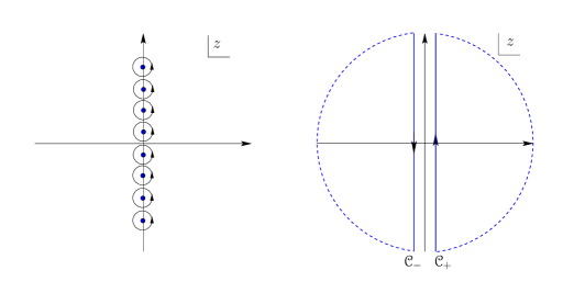
Figure 10: The left part shows the contour encircling the Matsubara frequencies. These contours can be deformed to the ones shown in the right part.

This formula can be interpreted in the following way. The first term is the vacuum amplitude and the second and third terms are the contributions from the thermally excited on-shell states, the second term represents roughly speaking the particles (positive energy states as measured by $\hat{H}$) and the third term represents the holes and anti-particles (negative energy states as measured by $\hat{H}$). The first integral, is of course, in general divergent and well defined only with a suitably chosen regularization. Note also that the second and third terms vanish at $T=0$.

Were we to take the Hamiltonian $\hat{H}$ as the fundamental one, then the first integral would indeed be the vacuum contour corresponding to it. However, we are rather interested in expressing the result in terms of the vacuum of the Hamiltonian $H_{0}$. Therefore it is necessary to express the Matsubara sum not in terms of the function $f_{\mu}$ but rather of $f$. We note that $\mathrm{Res}(f_{\mu})(\hat{z}_{k})=\mathrm{Res}(f)(z_{k})$ with $\hat{z}_{k}=z_{k}-\mu$, and therefore

$$T\sum_{n}f_{\mu}(z)=i\int_{-\infty}^{+\infty}\frac{dk_{0}}{2\pi}f(k_{0}+\mu+i\epsilon\,\mathrm{sgn}(k_{0}))+\sum_{z_{k}-\mu>0}\mathrm{Res}\left(f(z_{k})\right)n_{f}\left(\frac{z_{k}-\mu}{T}\right)-\sum_{z_{l}-\mu<0}\mathrm{Res}\left(f(z_{l})\right)n_{f}\left(\frac{\mu-z_{l}}{T}\right)\,.$$ (197)

Now we express the first contour in terms of the vacuum contour corresponding to the Hamiltonian $H_{0}$. This is the contour for which the poles with $z<0$ lie above and the poles with $z>0$ lie below. The difference between the vacuum contours corresponding to the Hamiltonians $\hat{H}$, $H_{0}$ is a contour enclosing all poles between $z=0$ and $z=\mu$ (see Figure 11),

$$i\int_{-\infty}^{+\infty}\frac{dk_{0}}{2\pi}f(k_{0}+\mu+i\epsilon\,\mathrm{sgn}(k_{0}))=i\int_{-\infty}^{+\infty}\frac{dk_{0}}{2\pi}f(k_{0}+\mu+i\epsilon\,\mathrm{sgn}(k_{0}+\mu))+\oint_{\mathcal{C}_{\mu}}\frac{dz}{2\pi i}f(z)\,.$$ (198)

Now we have succeeded in expressing the sum over Matsubara frequencies as a sum of a vacuum integral, the finite density contribution and the thermal fluctuations. Note that the poles of $f$ inside the contour $\mathcal{C}_{\mu}$ are precisely those poles for which either $z_{k}>0$ and $z_{k}-\mu<0$ for positive $\mu$ or $z_{l}<0$ and $z_{l}-\mu>0$ for negative $\mu$. Using $n_{f}(-x)=1-n_{f}(x)$ for these poles in the thermal sums we can express the amplitude as

$$T\sum_{n}f_{\mu}(z)=i\int_{-\infty}^{+\infty}\frac{dk_{0}}{2\pi}f(k_{0}+\mu+i\epsilon\,\mathrm{sgn}(k_{0}+\mu))+\sum_{z_{k}>0}\mathrm{Res}\left(f(z_{k})\right)n_{f}\left(\frac{z_{k}-\mu}{T}\right)-\sum_{z_{l}<0}\mathrm{Res}\left(f(z_{l})\right)n_{f}\left(\frac{\mu-z_{l}}{T}\right)\,.$$ (199)

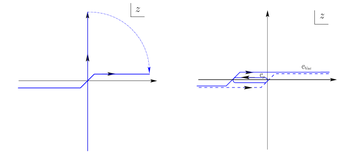
Figure 11: The Euclidean vacuum contour can be Wick rotated to a Lorentzian one. By another contour deformation is written as the vacuum contour of the normal ordered vacuum of the Hamiltonian $H_{0}$ (possibly in the gauge $A_{0}=\mu$ plus a finite contour enclosing the poles corresponding to the occupied states up to $k_{0}=\mu$.

The thermal sums over the residues are expressed now in terms of the particles and anti-particles according to the usual normal ordering prescription, i.e. the Hamiltonian $H_{0}$. They do not vanish at $T=0$ since they implicitly contain the finite density contribution.

Let us now use another way of defining the sum over Matsubara frequencies. We could also write

$$T\sum_{n}f(i\omega_{n}+\mu)=\frac{1}{2}\oint\frac{dz}{2\pi i}f(z)\tanh\left(\frac{z-\mu}{2T}\right)\,.$$ (200)

The only difference now is that the contours enclosing the poles of the hyperbolic tangent all are centered at $\mathop{\rm Re}(z)=\mu$. Going through the same steps as before we now end up with

$$T\sum_{n}f_{\mu}(z)=i\int_{-\infty}^{+\infty}\frac{dk_{0}}{2\pi}f(k_{0}+i\epsilon\,\mathrm{sgn}(k_{0}))+\sum_{z_{k}>0}\mathrm{Res}\left(f(z_{k})\right)n_{f}\left(\frac{z_{k}-\mu}{T}\right)-\sum_{z_{l}<0}\mathrm{Res}\left(f(z_{l})\right)n_{f}\left(\frac{\mu-z_{l}}{T}\right)\,.$$ (201)

The difference between (199) and (201) is simply a shift in the integration coordinate $z$ or $k_{0}$ respectively. Such a shift in momentum can also be understood as a gauge-transformation, if we assume for the moment that the symmetry generated by the charge $Q$ is gauged. The shift in the integration variable $k_{0}$ is then equivalent to a gauge transformation with a time dependent gauge parameter $\lambda=\mu t$. This introduces the gauge field $A_{0}=\mu$ into the theory. Note, however, that this gauge transformation does not change anything in the contours we used to define the Matsubara sums. The presence of the chemical potential is not related to the presence of a gauge field $A_{0}=\mu$ but rather to the way the poles of the function $f$ are circumvented in the complex energy plane.

Since (199) and (201) are related by the gauge transformation $\lambda=\mu t$, we should ask now what happens if the symmetry under consideration is anomalous, as this is the case of interest in this paper. To be specific we consider a chemical potential for the axial symmetry. It is well known that the axial anomaly for one Dirac fermion takes the form

$$\delta_{5}W_{\mathrm{eff}}[A,g]=\int\sqrt{|g|}\lambda_{5}\epsilon^{\mu\nu\rho\lambda}\left[\frac{1}{48\pi^{2}}\left(F^{5}_{\mu\nu}F^{5}_{\rho\lambda}+3F_{\mu\nu}F_{\rho\lambda}\right)+\frac{1}{384\pi^{2}}R^{\alpha}\,_{\beta\mu\nu}R^{\beta}\,_{\alpha\rho\lambda}\right]\,,$$ (202)

where $\delta_{5}$ is an axial transformation with parameter $\lambda_{5}$. We have introduced (so far non-dynamical) gauge fields for the axial, vector and diffeomorphism symmetry, $A^{5}_{\mu}$, $A_{\mu}$ and the metric $g_{\mu\nu}$. The anomaly is actually the sum of the pure axial anomaly given by the terms with the axial field strength $F^{5}_{\mu\nu}$, the mixed axial-vector anomaly and the mixed axial-gravitational anomaly. All anomalies have been shifted into the axial current. This implies a specific regularization scheme in evaluating the vacuum graph in (201).

Let us see what are the consequences of using either (199) or (201) for evaluating the Kubo formulas for anomalous transport in the presence of an axial chemical potential $\mu_{5}$. The gauge parameter relating the two is $\lambda_{5}=\mu_{5}t$. If we define the currents as the functional derivatives of the effective action, then the anomaly (202) will give new contributions beyond the common terms captured by the thermal sums of the residues. We are only interested here matching our results up to terms of first order in derivatives on the background fields. It follows that at this order of derivatives the mixed axial-gravitational anomaly will not contribute. We will further specify to the case where only a magnetic field $B_{i}=-\frac{1}{2}\epsilon^{0ijk}F_{jk}$ is present.

It is now straightforward to see that the contribution of (202), which arises from the vacuum integral in formula (199) is given by

$$\vec{J}_{\mathrm{vac}}=-\frac{\mu_{5}}{2\pi^{2}}\vec{B}\,.$$ (203)

The perturbative evaluation of the vacuum graph in (199) can be done by expanding in $\mu_{5}$. At first order one encounters a triangle diagram with $\mu_{5}$ sitting at one of the vertices. This diagram has been explicitly evaluated in Gynther et al. (2011) with the result (203). This is precisely the negative of the chiral magnetic effect stemming from the finite $T,\mu_{5}$ contribution! Therefore the total chiral magnetic effect vanishes if formula (199) is used for the axial chemical potential. This was first noticed in a holographic context in Rebhan et al. (2010). Therefore one needs to distinguish between the axial chemical potential and the axial background gauge field. Since axial gauge fields are absent on a fundamental level in nature we therefore advocate to use formula (201).

In the presence of anomalies the current defined as the variation of the effective action with respect to the gauge field is called the consistent current (because the anomaly (202) has to fulfill the Wess-Zumino consistency condition). This current is not invariant under the anomalous gauge transformation. But it is possible to define a current that is invariant under all gauge transformations, anomalous and non-anomalous ones by adding suitably chosen Chern-Simons currents. The axial gauge variation of the electric current follows from (202) as

$$\delta_{5}J^{\mu}=\frac{1}{4\pi^{2}}\epsilon^{\mu\nu\rho\lambda}\partial_{\nu}\lambda_{5}F_{\rho\lambda}\,.$$ (204)

There is, of course, nothing wrong with this. Axial transformations are not a symmetry and so there is no reason for the (consistent) current to be invariant. However it is now easy to define an invariant current by adding the Chern-Simons current

$$J^{\mu}_{\mathrm{cov}}=J^{\mu}-\frac{1}{4\pi^{2}}\epsilon^{\mu\nu\rho\lambda}A^{5}_{\nu}F_{\rho\lambda}\,.$$ (205)

This current is invariant under the usual gauge transformations and also under axial transformations. The covariant current is not conserved, rather it fulfills

$$\partial_{\mu}J^{\mu}_{\mathrm{cov}}=-\frac{1}{8\pi^{2}}\epsilon^{\mu\nu\rho\lambda}F^{5}_{\mu\nu}F_{\rho\lambda}\,.$$ (206)

We also note that in the absence of an axial background gauge field the covariant expectation values of the consistent currents coincide. One can also introduce a covariant axial current via $J^{\mu}_{5,\mathrm{cov}}=J^{\mu}_{5}-\frac{1}{12\pi^{2}}\epsilon^{\mu\nu\rho\lambda}A^{5}_{\nu}F_{\rho\lambda,5}$.

We intend now to give a physical interpretation of the consistent and covariant currents. From equation (199) we see that the finite temperature and density contributions are given by well defined expressions. Integrals over spatial momenta are regulated by the presence of the Fermi-Dirac distributions. All contributions to the current stemming from them are automatically invariant. Therefore we identify the current produced by the physically moving charges, i.e. the collective motion of the on-shell states, as the contributions to the covariant current. The covariant anomaly (206) states that in parallel electric and magnetic fields of axial and vector type charged particles are created out of the vacuum via spectral flow. More precisely, for every finite ultraviolet cutoff particles are flowing into the physical region below that cutoff via the spectral flow induced by the parallel electric and magnetic fields.

The covariant current is, however, not the one that couples to the (vector) gauge field $A_{\mu}$. This is by definition the consistent current with exactly vanishing divergence. If we give dynamics to the vector field by adding a Maxwell term to the effective action, it is the consistent current that enters Maxwell’s equation

$$J^{\nu}=\partial_{\mu}F^{\mu\nu}\,,$$ (207)

whereas the covariant current enters in a Chern-Simons modification of Maxwell’s equation

$$J^{\nu}_{\mathrm{cov}}=\partial_{\mu}F^{\mu\nu}-\frac{1}{4\pi^{2}}\epsilon^{\nu\mu\rho\lambda}A^{5}_{\mu}F_{\rho\lambda}\,.$$ (208)

Let us summarize now the response to a magnetic field in the covariant, the consistent and the energy currents. We also keep now the notion of chemical potential and (axial) vector potential apart but do include the presence of constant $A^{5}_{0}$. Then

$$\vec{J}_{\mathrm{cons}} =\frac{\mu_{5}-A^{5}_{0}}{2\pi^{2}}\vec{B}\,,$$ (209)

$$\vec{J}_{\mathrm{cov}} =\frac{\mu_{5}}{2\pi^{2}}\vec{B}\,,$$ (210)

$$\vec{J}_{\epsilon} =\frac{\mu\mu_{5}}{2\pi^{2}}\vec{B}\,.$$ (211)

Note that the energy flow does not depend on the axial gauge field background! In fact even upon using (199) the Kubo formula for the energy flow does not depend on the presence of a background axial gauge field because the perturbative expansion of the vacuum amplitude involves a triangle diagram of the form $\langle T^{0i}J^{j}J_{5}^{0}\rangle A_{0}^{5}$. This triangle diagram does not have an anomalous contribution and is therefore insensitive to a constant $A_{0}^{5}$. So in the absence of $\mu_{5}$ there is no energy flow connected to the presence of the consistent current (209). Moreover, notice that if one chooses $A_{0}^{5}=\mu_{5}$ one gets a vanishing chiral magnetic effect in the consistent current but a non-vanishing result in the energy current!.

A related aspect concerns the energy-momentum conservation in the presence of external background gauge fields. It follows from the Ward identity for diffeomorphisms (165) which can be written as

$$\partial_{\mu}T^{\mu\nu}=F^{\nu\mu}J_{\nu}+F_{5}^{\nu\mu}J^{5}_{\mu}-\frac{A^{\nu}_{5}}{48\pi^{2}}\epsilon^{\mu\lambda\rho\sigma}\left(\ 3F_{\mu\lambda}F_{\rho\sigma}+F^{5}_{\mu\lambda}F^{5}_{\rho\sigma}\right)=0\,.$$ (212)

Evaluating this in a frame where there is no energy current in the background of vanishing axial field strength but presence of the chiral magnetic current (209) we find that the contributions from the axial background field vanish and therefore

$$\partial_{t}T^{00}=\frac{\mu_{5}-A_{0}^{5}}{2\pi^{2}}\vec{E}\vec{B}+\frac{A_{0}^{5}}{2\pi^{2}}\vec{E}\vec{B}=\frac{\mu_{5}}{2\pi^{2}}\vec{E}\vec{B}\,.$$ (213)

This seems natural since we have seen already in (211) that the axial background field does not contribute to the energy transport. In fact the cancellation is more generally valid. The energy momentum conservation is most conveniently expressed in terms of the covariant currents as

$$\partial_{\mu}T^{\mu\nu}=F^{\nu\mu}J_{\mu,\mathrm{cov}}+F_{5}^{\nu\mu}J_{\mu,\mathrm{cov}}^{5}\,.$$ (214)

One possible point of view is therefore that the Chern-Simons current $J^{\mu}_{CS}=\epsilon^{\mu\nu\rho\lambda}A^{5}_{\nu}F_{\rho\lambda}$ is not a genuine transport phenomenon. Rather we might take it as the necessity to modify Maxwell’s equations in a quantum vacuum of chiral fermions by adding a Chern-Simons current as in (208)!

References

- Abelev et al. (2009) B. I. Abelev et al. (STAR), Phys. Rev. Lett. 103, 251601 (2009), arXiv:0909.1739 [nucl-ex] . %%CITATION = 0909.1739;%%
- Abelev et al. (2013) B. Abelev et al. (ALICE Collaboration), Phys.Rev.Lett. 110, 012301 (2013), arXiv:1207.0900 [nucl-ex] .
- Fukushima (2013) K. Fukushima, Lect.Notes Phys. 871, 241 (2013), arXiv:1209.5064 [hep-ph] .
- Vilenkin (1995) A. Vilenkin, Astrophys.J. 451, 700 (1995).
- Vilenkin (1980a) A. Vilenkin, Phys.Rev. D22, 3080 (1980a).
- Giovannini and Shaposhnikov (1998) M. Giovannini and M. Shaposhnikov, Phys.Rev. D57, 2186 (1998), arXiv:hep-ph/9710234 [hep-ph] .
- Alekseev et al. (1998) A. Y. Alekseev, V. V. Cheianov, and J. Fröhlich, Phys. Rev. Lett. 81, 3503 (1998), arXiv:cond-mat/9803346 . %%CITATION = COND-MAT/9803346;%%
- Son and Zhitnitsky (2004) D. T. Son and A. R. Zhitnitsky, Phys. Rev. D70, 074018 (2004), arXiv:hep-ph/0405216 . %%CITATION = HEP-PH/0405216;%%
- Metlitski and Zhitnitsky (2005) M. A. Metlitski and A. R. Zhitnitsky, Phys. Rev. D72, 045011 (2005), arXiv:hep-ph/0505072 . %%CITATION = HEP-PH/0505072;%%
- Newman and Son (2006) G. M. Newman and D. T. Son, Phys. Rev. D73, 045006 (2006), arXiv:hep-ph/0510049 . %%CITATION = HEP-PH/0510049;%%
- Kharzeev and Zhitnitsky (2007) D. Kharzeev and A. Zhitnitsky, Nucl.Phys. A797, 67 (2007), arXiv:0706.1026 [hep-ph] .
- Erdmenger et al. (2009) J. Erdmenger, M. Haack, M. Kaminski, and A. Yarom, JHEP 01, 055 (2009), arXiv:0809.2488 [hep-th] . %%CITATION = 0809.2488;%%
- Banerjee et al. (2011) N. Banerjee et al., JHEP 01, 094 (2011), arXiv:0809.2596 [hep-th] .
- Son and Surowka (2009) D. T. Son and P. Surowka, Phys. Rev. Lett. 103, 191601 (2009), arXiv:0906.5044 [hep-th] .
- Kharzeev and Warringa (2009) D. E. Kharzeev and H. J. Warringa, Phys. Rev. D80, 034028 (2009), arXiv:0907.5007 [hep-ph] . %%CITATION = 0907.5007;%%
- Amado et al. (2011) I. Amado, K. Landsteiner, and F. Pena-Benitez, JHEP 1105, 081 (2011), arXiv:1102.4577 [hep-th] .
- Landsteiner et al. (2013) K. Landsteiner, E. Megias, and F. Pena-Benitez, Lect.Notes Phys. 871, 433 (2013), arXiv:1207.5808 [hep-th] .
- Yee (2009) H.-U. Yee, JHEP 11, 085 (2009), arXiv:0908.4189 [hep-th] . %%CITATION = 0908.4189;%%
- Chen et al. (2013) Y. Chen, S. Wu, and A. A. Burkov, Phys. Rev. B 88, 125105 (2013), arXiv:1306.5344 [cond-mat.mes-hall] .
- Landsteiner et al. (2011a) K. Landsteiner, E. Megias, and F. Pena-Benitez, Phys. Rev. Lett. 107, 021601 (2011a), arXiv:1103.5006 [hep-ph] .
- Neiman and Oz (2011) Y. Neiman and Y. Oz, JHEP 03, 023 (2011), arXiv:1011.5107 [hep-th] .
- Vilenkin (1980b) A. Vilenkin, Phys.Rev. D21, 2260 (1980b).
- Landsteiner et al. (2011b) K. Landsteiner, E. Megias, L. Melgar, and F. Pena-Benitez, JHEP 1109, 121 (2011b), arXiv:1107.0368 [hep-th] .
- Loganayagam and Surowka (2012) R. Loganayagam and P. Surowka, JHEP 1204, 097 (2012), arXiv:1201.2812 [hep-th] .
- Chapman et al. (2012) S. Chapman, Y. Neiman, and Y. Oz, JHEP 1207, 128 (2012), arXiv:1202.2469 [hep-th] .
- Gao et al. (2012) J.-H. Gao, Z.-T. Liang, S. Pu, Q. Wang, and X.-N. Wang, Phys.Rev.Lett. 109, 232301 (2012), arXiv:1203.0725 [hep-ph] .
- Jensen et al. (2013a) K. Jensen, R. Loganayagam, and A. Yarom, JHEP 1302, 088 (2013a), arXiv:1207.5824 [hep-th] .
- Megias and Pena-Benitez (2013a) E. Megias and F. Pena-Benitez, JHEP 1305, 115 (2013a), arXiv:1304.5529 [hep-th] .
- Megias et al. (2013) E. Megias, K. Landsteiner, and F. Pena-Benitez, Acta Phys.Polon.Supp. 6, 45 (2013).
- Megias and Pena-Benitez (2013b) E. Megias and F. Pena-Benitez, (2013b), arXiv:1307.7592 [hep-th] .
- Golkar and Son (2012) S. Golkar and D. T. Son, (2012), arXiv:1207.5806 [hep-th] .
- Gorbar et al. (2013) E. Gorbar, V. Miransky, I. Shovkovy, and X. Wang, Phys.Rev. D88, 025025 (2013), arXiv:1304.4606 [hep-ph] .
- Hou et al. (2012) D.-F. Hou, H. Liu, and H.-c. Ren, Phys.Rev. D86, 121703 (2012), arXiv:1210.0969 [hep-th] .
- Zakharov (2013) V. I. Zakharov, Lect.Notes Phys. 871, 295 (2013), arXiv:1210.2186 [hep-ph] .
- Jensen et al. (2013b) K. Jensen, P. Kovtun, and A. Ritz, (2013b), 10.1007/JHEP10(2013)186, arXiv:1307.3234 [hep-th] .
- Kharzeev and Son (2011) D. E. Kharzeev and D. T. Son, Phys. Rev. Lett. 106, 062301 (2011), arXiv:1010.0038 [hep-ph] .
- Keren-Zur and Oz (2010) B. Keren-Zur and Y. Oz, JHEP 06, 006 (2010), arXiv:1002.0804 [hep-ph] . %%CITATION = 1002.0804;%%
- Rebhan et al. (2010) A. Rebhan, A. Schmitt, and S. A. Stricker, JHEP 01, 026 (2010), arXiv:0909.4782 [hep-th] . %%CITATION = 0909.4782;%%
- Landsman and van Weert (1987) N. Landsman and C. van Weert, Phys.Rept. 145, 141 (1987).
- Manes and Valle (2013) J. L. Manes and M. Valle, JHEP 1301, 008 (2013), arXiv:1211.0876 [hep-th] .
- Le Bellac (1996) M. Le Bellac, Thermal Field Theory, Cambridge University Press (1996).
- Fukushima et al. (2008) K. Fukushima, D. E. Kharzeev, and H. J. Warringa, Phys. Rev. D78, 074033 (2008), arXiv:0808.3382 [hep-ph] . %%CITATION = 0808.3382;%%
- Landsteiner and Melgar (2012) K. Landsteiner and L. Melgar, JHEP 1210, 131 (2012), arXiv:1206.4440 [hep-th] .
- Son and Starinets (2002) D. T. Son and A. O. Starinets, JHEP 0209, 042 (2002), arXiv:hep-th/0205051 [hep-th] .
- Kaminski et al. (2010) M. Kaminski, K. Landsteiner, J. Mas, J. P. Shock, and J. Tarrio, JHEP 02, 021 (2010), arXiv:0911.3610 [hep-th] . %%CITATION = 0911.3610;%%
- Gynther et al. (2011) A. Gynther, K. Landsteiner, F. Pena-Benitez, and A. Rebhan, JHEP 02, 110 (2011), arXiv:1005.2587 [hep-th] .
- Satow and Yee (2014) D. Satow and H.-U. Yee, (2014), arXiv:1406.1150 [hep-ph] .
- Evans (1995) T. S. Evans, (1995), arXiv:hep-ph/9510298 .
- Buividovich (2014) P. Buividovich, Nucl.Phys. A925, 218 (2014), arXiv:1312.1843 [hep-lat] .
- Kirilin et al. (2013) V. Kirilin, A. Sadofyev, and V. Zakharov, (2013), arXiv:1312.0895 [hep-th] .