Tunable strong nonlinearity of a micromechanical beam embedded in a dc-SQUID

Abstract

We present a study of the controllable nonlinear dynamics of a micromechanical beam coupled to a dc-SQUID (superconducting quantum interference device). The coupling between these systems places the modes of the beam in a highly nonlinear potential, whose shape can be altered by varying the bias current and applied flux of the SQUID. We detect the position of the beam by placing it in an optical cavity, which frees the SQUID to be used solely for actuation. This enables us to probe the previously unexplored full parameter space of this device. We measure the frequency response of the beam and find that it displays a Duffing oscillator behavior which is periodic in the applied magnetic flux. To account for this, we develop a model based on the standard theory for SQUID dynamics. In addition, with the aim of understanding if the device can reach nonlinearity at the single phonon level, we use this model to show that the responsivity of the current circulating in the SQUID to the position of the beam can become divergent, with its magnitude limited only by noise. This suggests a direction for the generation of macroscopically distinguishable superposition states of the beam.

I Introduction

Micro and Nano-Electromechanical systems (NEMS and MEMS) have been a subject of intense research in the past decade Poot and van der Zant (2012); Ekinci et al. (2004); Lifshitz and M. C. Cross (2008); Karabalin et al. (2009); Kozinsky et al. (2007); LaHaye et al. (2009); Teufel et al. (2011a); Gröblacher et al. (2008), due to their potential for both probing fundamental physical questions, such as the limits of validity of quantum mechanics Teufel et al. (2011b); LaHaye et al. (2009); Agarwal and Eberly (2012), and for functioning as highly sensitive, quantum-limited detectors Buks et al. (2007); Ekinci and Roukes (2005); Etaki et al. (2011, 2008); Poot and van der Zant (2012). One of the appealing aspects of these devices is their tendency to display nonlinear behavior. This, in addition to providing an experimentally accessible testbed for studies of nonlinear dynamical systems Schwab (2002); Kozinsky et al. (2007); Karabalin et al. (2009); Dykman (2012); Lifshitz and M. C. Cross (2008); Defoort et al. (2014); Villanueva et al. (2013); Kenig et al. (2012), is a resource for the generation of nonclassical states of mechanical elements Yurke and Stoler (1986a); Yurke and Stoler (1986b); Katz et al. (2007, 2008); Ludwig et al. (2008); Qian et al. (2011); Xue et al. (2007).

A particular type of nonlinearity, that of a resonator with an amplitude-dependent spring constant (Duffing resonator), can be gainfully harnessed for this end: It has been shown that both the multi-phonon transitions it exhibits, as well as its inherent bistability, enable the generation of a superposition of macroscopically distinct coherent states Yurke and Stoler (1986a); Katz et al. (2007, 2008). It is therefore highly advantageous to be able to generate Duffing nonlinearity in NEMs and MEMs which is both strong and can be controlled, tuned, and detected by the experimenter.

In this work we demonstrate the possibility to achieve such a controllable nonlinearity in a mechanical beam embedded in a dc-SQUID and placed in an external magnetic field. The magnetomotive interaction of the SQUID with the beam places the latter in a highly nonlinear potential, which in particular gives rise to a Duffing nonlinearity. The shape of the potential, and with it the resonance frequency and Duffing coefficient of the beam modes, can be altered by varying the control parameters (bias current and applied bias flux) of the SQUID.

In previous work on a similar system Etaki et al. (2008); Poot et al. (2010); Etaki et al. (2011); Schneider et al. (2012); Etaki et al. (2013), the SQUID was used both to read out the position of the beam in addition to influencing its dynamics. As a result, the SQUID could only be biased at an operating point in which the voltage is sufficiently dependent on the flux to allow displacement detection. While this scheme provided a highly sensitive displacement measurement, it also placed a restriction on the range of control parameters that could be explored. In contrast, in our work displacement detection is independent of the SQUID, which enables us to explore the full space of control parameters of the device.

In our device, displacement detection is obtained by forming an optical cavity between the beam and the tip of an optical fiber placed directly above it Zaitsev et al. (2011) (see Fig. 1). The cavity is driven by a laser, and power reflected off of it is dependent on the displacement of the beam. To actuate the beam, we coat the tip of the fiber with Niobium and apply a biased AC voltage, which drives the beam capacitively (see Fig. 1). Using this scheme, we measure the frequency response of the fundamental beam mode near resonance, from which we extract the dependence of its resonance frequency and Duffing coefficient Kozinsky et al. (2007); Lifshitz and M. C. Cross (2008) on the control parameters of the SQUID.

Interestingly, we find that the resonance frequency and Duffing coefficient display pronounced periodic oscillations as the bias flux of the SQUID is varied (see Figs. 2 and 3), which can be directly attributed to the flux-periodic response of the SQUID. These oscillations change their shape as the bias current is varied, and their magnitude is largest near the transition from the zero voltage state (S-state) of the SQUID to its resistive state (R-state). A model, based on the standard theory of SQUID dynamics (RCSJ), is developed which accounts for the results. While most of the qualitative as well quantitative details of the measurements are reproduced by this model, several discrepancies exist, as shown in Fig. 4.

A specific and previously unattainable bias point of the SQUID, for which the nonlinearity is expected to be particularly strong, is at the transition to the resistive state when the bias flux is set at half-integer values in units of the magnetic flux quantum. We argue that as the bias current and applied bias flux of the SQUID approach this point, the induced resonance frequency shift and Duffing coefficient of the beam diverge, and that this divergence is physically limited by noise in the SQUID. Since this transition is in fact an infinite period bifurcation Strogatz (2001), in what follows we shall refer to this point as the bifurcation cusp point.

II The experiment

II.1 Overview of the system

Figure 1: (color online) A schematic description of the experimental system. The SQUID is biased with a current $I_{B}$, and the voltage across it is amplified and measured. The displacement of the mechanical modes, which are placed in a transverse magnetic field, is detected with an optical cavity. This cavity is formed by the beam on one side and the tip of the optical fiber (red) on the other. The fiber is coated with Niobium electrode, which is set, using a bias tee (not shown) at a finite dc voltage and connected to the reference output of an RF lock in amplifier. The power reflected from the cavity is converted to voltage with an RF photodetector, and then measured with the lock in amplifier. (a): A 3D blow-up of the SQUID, with the junctions shown in front. The fiber is located above one of the beams. The displacement of the measured beam mode is denoted by $u$, and the circulating current in the SQUID by $J$. The SQUID is fabricated in a Nb/AlOx/Nb configuration, and is top-coated with gold.

The device was created by patterning a dc-SQUID in a trilayer configuration on a SiN coated Si substrate Yuvaraj et al. (2011). A part of the SQUID loop was freed and suspended in vacuum, and functioned as a mechanical beam. The displacement of this beam was detected by placing an optical fiber above, which forms a cavity between the top of the SQUID and the fiber tip (see Fig. 1). While two beams were freed, our experiment focused on the dynamics of the fundamental mode of only one of them. The Josephson junctions (JJs), which were overdamped and non-hysteretic, were found to have an average critical current $I_{0}=317.5{\rm\mu A}$ at zero magnetic field. Further details regarding the SQUID, and definitions of SQUID parameters used subsequently for modeling the dynamics of the device, can be found in the appendices. The mechanical elements functioned as doubly-clamped beams of length $\ell=100{\rm\mu m}$. We measured the frequency response of the fundamental mode of one of the beams, which had an angular frequency $\omega_{0}=2\pi\times 311.75{\rm KHz}$ and quality factor $Q_{m}\simeq 6200$. The system was placed in an external magnetic field of $60{\rm mT}$ formed by a split-coil magnet. The field was aligned with the plane of the sample, although a small component perpendicular to the plane of the SQUID existed and contributed to the flux threading the loop.

II.2 Experiment and results

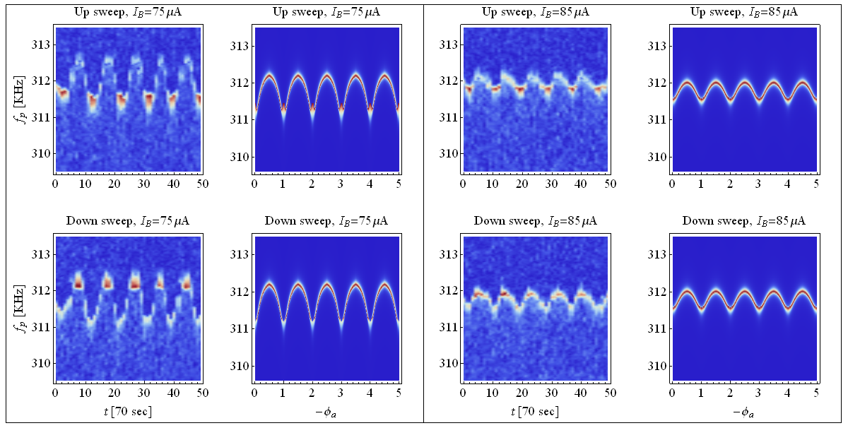
Figure 2: Comparison of frequency response measurements to the theoretical model. The left panel in each frame shows the experimental measurement and the right panel shows the theoretical prediction, obtained with the model outlined in section II.2. The up (down) sweeps correspond to the direction in which the frequency of the signal actuating the beam was altered. The abscissa is $-\phi_{a}$ in the theoretical panel since in the experiment the flux decreased with time. Blue (red) colors denote a weaker (stronger) response. The plots here show the frequency response when the system is fully in the R-state, for bias currents $I_{B}>2I_{0}$. The sinusoidal modulation in the resonance frequency of the beam and the hysteretic tilted Lorentzian response, which corresponds to a Duffing nonlinearity, are induced by the SQUID.

The influence of the SQUID on the beams was measured by obtaining the frequency response of the beams to a sinusoidal capacitive force near the resonant frequency of the fundamental mode. In the absence of the split coil magnetic field, the response of the mode was independent of the SQUID bias current $I_{B}$ and the applied flux $\Phi_{a}$. When the field was turned on and the bias currently was increased, the frequency response developed a pattern which had unique features for different values of $I_{B}$, which were periodic in the applied flux. (see Figs. 2, 3 and 4). The features were most pronounced near the transition from the S-state to the R-state of the SQUID, and subsequently began to decay as $I_{B}$ was further increased to the regime in which the SQUID displayed ohmic behavior. Note that the $\Phi_{a}$ was sweeped by allowing the magnetic field in the split coil magnet to freely decay and making use of the imperfect alignment of the field with the plane of the sample Schneider et al. (2012).

At $I_{B}=0$ the response of the beam mode to actuation could be fitted to a Lorentzian, indicative of a a harmonic response. As $I_{B}$ was increased, however, the response started to exhibit, in addition to a resonance frequency shift, a “tilted” Lorentzian characteristic of a Duffing oscillator. To verify this, the response was swept both in the up and down directions, and hysteretic response, indicative of a Duffing bistability, was clearly observed. Sharp transitions in the up and down sweeps correspond to an amplitude-dependent spring hardening and softening, respectively. For some values of control parameters, the hysteretic behavior was particularly pronounced, indicating a strong nonlinearity of the beam mode.

II.3 Discussion and theory

To understand the observed frequency response, we first outline the dynamics of a SQUID coupled to a vibrating beam Buks and Blencowe (2006); Blencowe and Buks (2007); Poot et al. (2010); Etaki et al. (2013). We denote the current in the arms of the SQUID by $I_{n}=I_{0,n}\sin\gamma_{n}$, where $n=1,2$, $I_{0,n}$ is the critical current in the $n$’th junction, and $\gamma_{i}$ is the gauge invariant phase across the junctions. Furthermore, denoting the component of the applied magnetic field in the plane of the SQUID as $B$, a Lorentz force $F_{L}=\lambda J\ell B$ acts on the beams, where $\lambda$ is a correction factor accounting for the mode shape (see appendix and Nation et al. (2008); Blencowe and Buks (2007)) and $J=(I_{1}-I_{2})/2$ is the circulating current in the SQUID. Concurrently, the total flux $\Phi$ threading the SQUID is dependent on the displacement of the beams. To first order, we have $\Phi=\Phi_{a}+\lambda B\ell x+LJ$, where $x$ is the displacement of the driven mechanical mode from its equilibrium position, $\Phi_{a}$ is the applied flux threading the SQUID loop at $x=0$ and $L$ is the self inductance of the loop. Since $x\ll\ell$ and $\Phi_{a}\gg LJ$, we can make the approximation $\dot{\Phi}\simeq\lambda B\ell\dot{x}+L_{0}\dot{J}$, where $L_{0}$ is the loop inductance when the beams are in their equilibrium positions.

Since the Lorentz force acting on the mode depends on its displacement, it is placed in an potential whose shape depends on the control parameters of the SQUID. By measuring the mechanical resonance frequency shift and Duffing nonlinearity, the observed frequency response allows us to extract the quadratic and quartic terms of this potential around the equilibrium point. To calculate the Lorentz force acting on the beam, we find the circulating current in the SQUID for the given control parameters, and assume that the mechanical displacement is a small perturbation of the applied flux. Since the oscillation frequency of the SQUID $\omega_{c}=2\pi RI_{0}/\Phi_{0}\gg\omega_{0}$, we only need to consider the dc component of the circulating current.

We assume that the equation of motion for the amplitude of the driven mode, in normalized units, is given by

$$\ddot{u}+\kappa_{m}\dot{u}+\omega_{0}^{2}u=g^{2}j_{\mathrm{av}}(\phi_{a}+u,i_{B})+h_{d}\cos\omega_{p}t,$$ (1)

where $u=x/x_{B}$, overdot denotes time derivative, $\kappa_{m}=\omega_{0}/Q_{m}$, $g=\lambda\ell B\sqrt{I_{0}/m_{{\rm eff}}\Phi_{0}}$, $i_{B}=I_{B}/I_{0}$, $I_{B}=I_{1}+I_{2}$, $\phi_{a}=\Phi_{a}/\Phi_{0}$ is the normalized applied flux, $h_{d}$ is the normalized driving strength and $\omega_{p}$ is the driving signal angular frequency. Here $x_{B}=\Phi_{0}/\lambda\ell B$ is the displacement required to change the applied flux by $\Phi_{0}=h/2e$, $m_{{\rm eff}}$ is the effective mass of the mode, and $j_{\mathrm{av}}=J_{{\rm av}}/I_{0}$ is the averaged and normalized circulating current. In the S-state $j_{\mathrm{av}}$ is determined by the location of the stable equilibrium points (wells) of the SQUID potential, and in the R-state it is given by $j_{\mathrm{av}}=\Theta^{-1}\int_{0}^{\Theta}j(t){\rm d}t$, where $\Theta$ is a single period of $j(t)=J(t)/I_{0}$. The coordinate $u$ can be treated adiabatically when solving for the dynamics of the SQUID since the latter is overdamped and $g^{2}/\omega_{c}\omega_{0}\ll Q_{m}^{-1}$ Schwab (2002); Poot et al. (2010), where $\omega_{c}$ is the JJ oscillation frequency at the R-state. Since the SQUID dynamics are highly nonlinear and in the R-state no stable equilibrium points exist, the general analytical calculation of $j_{\mathrm{av}}$ in both states is difficult, and so we obtain it numerically (see appendix B). We then find the mode frequency shift and Duffing coefficient by assuming that $u\ll 1$ and expanding $j_{\mathrm{av}}$ in powers of $u$.

We can see that above the S-state, in Figs. 2 and 3, the predicted frequency shift follows the experimental data closely. However, the Duffing nonlinearity is only in partial agreement with the data. For example, in Fig. 3, for $I_{B}=75{\rm\mu A}$, the nonlinearity appears to be symmetric, while the theory suggests that it should be observable only at integer flux quanta. A larger discrepancy between theory and experiment is found in Fig. 4, which is for a low bias current, for which the SQUID is in the S-state for all values of $\phi_{a}$. For $I_{B}<I_{c,{\rm min}}$, the minimal critical current, the SQUID potential has a multiplicity of stable wells. As $\phi_{a}$ is varied, these wells disappear and reappear periodically. The theoretical prediction is that the force on the beams due to circulating current is approximately linear for most values of $\phi_{a}$, except near those points in which a well in the SQUID potential disappears. Thus, the Lorentz force acting on the beams should be linear except near values of $\phi_{a}$ in which a dip in mechanical frequency should occur. The measured frequency response, however, does not exhibit these dips.

Note that an important consequence of the model described by Eq. (1), is that $j_{\mathrm{av}}$ is a function of the sum $\phi_{a}+u$. Due to this, the sign and magnitude of the Duffing coefficient should be proportional to the second derivative of the frequency shift. This feature is qualitatively consistent with the experimental data shown in the panels of Figs. 2 and 3.

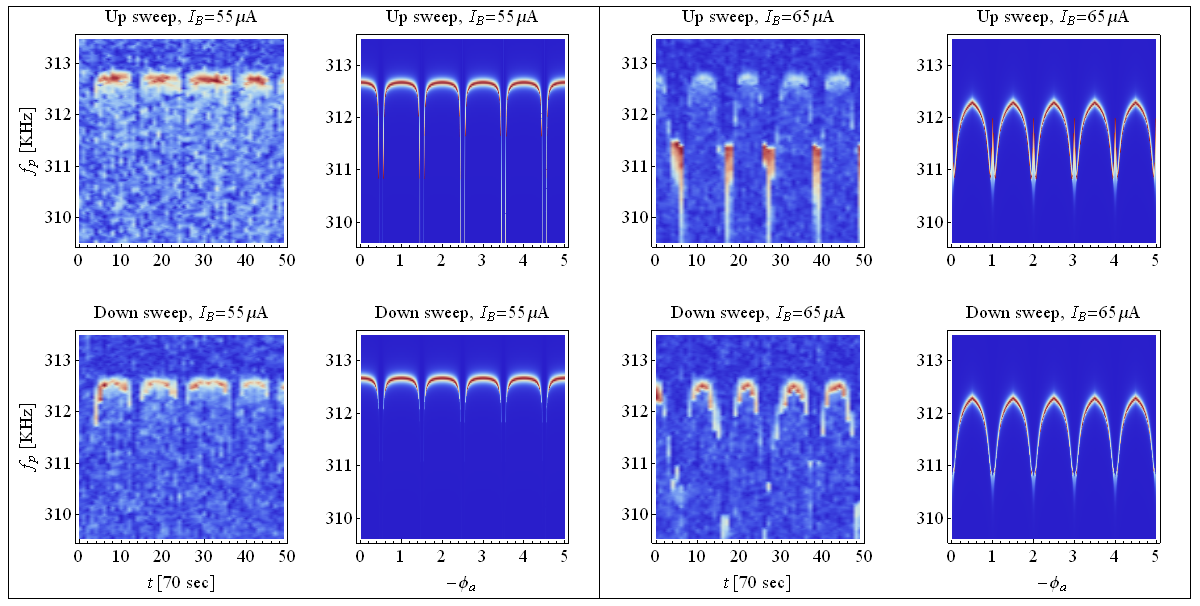
Figure 3: (Continued from Fig. 2.) Frequency response lower values of SQUID bias current. The average critical current of each JJ with applied magnetic field is $I_{0}=30\pm 2{\rm\mu A}$, and since $\beta_{L}=4$ in magnetic field, we have $I_{c,{\rm min}}=49\pm 3{\rm\mu A}$. Thus, in the plot at $I_{B}=55{\rm\mu A}$, the SQUID is in the S-state most of the time, and the sharp dip in the frequency of the beam corresponds to the bifurcation cusp point.

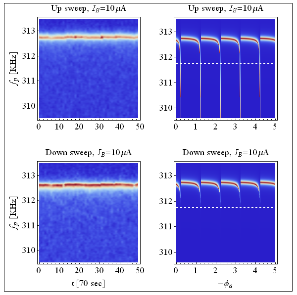
Figure 4: (color online) Frequency response of the driven mechanical mode to capacitive actuation, when the bias current $I_{B}$ is smaller than $I_{c,{\rm min}}$. In this case the SQUID is in the S-state for all values of $\phi_{a}$. The white dashed line at $f_{p}=311.75{\rm KHz}$ corresponds to the resonance frequency of the mechanical mode for the case $B=0$. The discrepancy between theoretical prediction and experimental measurements is discussed in subsection II.2. Response for higher bias currents is shown in Figs. 2 and 3.

III Dynamics near the bifurcation cusp point

III.1 Maximal attainable nonlinearity

Since we have seen that very strong nonlinearity is exhibited in this device, it is interesting to consider for which values of the control parameters this effect is most pronounced. To address this question, we consider a symmetric dc-SQUID with $\beta_{L}\lesssim 1$ and normalized capacitance $\beta_{c}\ll 1$, which makes the analysis tractable without changing the results qualitatively. The normalized bias current $i_{c}(\phi_{a})$ for which a transition to the R-state occurs is a periodic function of the normalized applied flux $\phi_{a}$ with period 1, and its minimal value $i_{c,{\mathrm{min}}}$ occurs at $\phi_{a}=\frac{1}{2}+n$, where $n$ is an integer. Setting $\delta\phi=\phi_{a}-\frac{1}{2}$, and $\delta i=i_{B}-i_{c,{\rm min}}$, we focus on the dynamics of the SQUID close to the bifurcation cusp point $\delta\phi=0$, $\delta i=0$. When the SQUID is biased near this point, the circulating current $j_{\mathrm{av}}$ becomes extremely sensitive to the applied flux since for $\delta\phi>0$ ($\delta\phi<0$) it is energetically more favorable for $j_{\mathrm{av}}$ to be large and negative (positive), and so the point $\delta\phi=0$ exhibits a singularity which remains also in a modestly asymmetric SQUID. In the R-state, the jump in $j_{\mathrm{av}}$ must occur on a span of $\delta\phi$ which is on the order of $\delta i$. From this we may anticipate that $\partial^{n}j_{\mathrm{av}}/\partial\phi_{a}^{n}\propto(\delta i)^{-n}$. To verify this, we calculate $j_{\mathrm{av}}$ for $|\delta\phi|\ll 1$ and $0<\delta i\ll 1$. Assuming $\beta_{L}\ll 1$, we may use adiabatic elimination to set $j=-\cos\left(\frac{\gamma}{2}\right)+O(\beta_{L})$, where $\gamma=\gamma_{1}+\gamma_{2}$, and reduce the dynamics near $\phi_{a}=\frac{1}{2}$ to the one-dimensional equation ${\rm d}\gamma/{\rm d}\tau=-{\rm d}v/{\rm d}\gamma+O(\beta_{L}^{2}),$ where

$$v(\gamma)=4\pi\delta\phi\cos\left(\frac{\gamma}{2}\right)-\frac{1}{2}\pi\beta_{L}\cos\left(\gamma\right)-i_{B}\gamma$$ (2)

and $\tau=\omega_{c}t$. This equation describes overdamped motion of $\gamma$ in a “double” washboard potential. When $0<\delta i\ll 1$ and $|\delta\phi|\ll 1$, this potential no longer contains any wells. It does, however, contain nearly flat regions around the points $\gamma_{c}$, defined by $v^{\prime\prime}(\gamma_{c})=0$ and $v^{\prime\prime\prime}(\gamma_{c})<0$, in which the dynamics are slow. In fact, during a single period $\Theta$ of $j$, the time spent away from these points scales as $\sqrt{\delta i}$, and so it is sufficient to solve for the dynamics around them.

Restricting our attention to $-2\pi\leq\gamma\leq 2\pi$, a single period of $v(\gamma)+i_{B}\gamma$, we have two such points, which we denote as $\gamma_{c\pm}$. If we expand the potential around them and keep terms up to quadratic order, we may solve the resulting equations and find an approximate analytical expression for $j_{\mathrm{av}}$, which is correct up to an error of $O(\sqrt{\delta i})$. A plot of $j_{\mathrm{av}}$ obtained using this analytical expression is given in Fig. 5, and its explicit form can be found in appendix C. Expanding this expression around $\delta\phi=0$, and making the additional assumption that $\delta i\ll\beta_{L}$, we find that

$$j_{{\rm av}}(\delta\phi)=\frac{\pi}{2\sqrt{2}}\frac{\delta\phi}{\delta i}+\frac{\pi^{3}}{4\sqrt{2}}\left(\frac{\delta\phi}{\delta i}\right)^{3}+\frac{\pi^{5}}{4\sqrt{2}}\left(\frac{\delta\phi}{\delta i}\right)^{5}+\dots$$ (3)

as we anticipated from the qualitative reasoning of the previous paragraph ($\partial^{n}j_{\mathrm{av}}/\partial\phi_{a}^{n}\propto(\delta i)^{-n}$). We numerically find that this result remains qualitatively valid even when $\beta_{L}$ is not small.

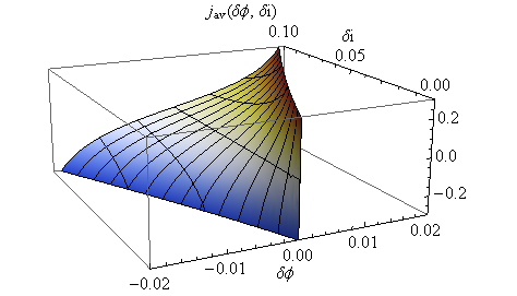
Figure 5: (color online) The average circulating current in the region $0<\delta i\ll 1$, as given by the analytical approximation (see Eq. 12). The singular behavior at the cusp point ($\delta i=0$, $\delta\phi=0$) is evident (3). This behavior can be exploited for the generation of highly nonlinear response of the beam modes.

III.2 Fundamental limits on the divergence of the Duffing coefficient

The above discussion on the divergence of $\delta i$ disregards thermal noise and $1/f$ noise. In reality, these noises render the limit $\delta i\to 0$ unphysical. First, we consider the limitation set by thermal noise. This can be accounted for by adding a white noise term to the equation for $\gamma$. We then obtain a nonlinear Langevin equation with a critical point of the marginal type Kubo et al. (1973); Colet et al. (1989); Caceres et al. (1995). A simple dimensional analysis argument indicates that when $\delta i=0$, a noise-induced transition from $\gamma_{c+}$ to $\gamma_{c-}$ should occur on a time scale $\tau_{N}\propto(|v^{\prime\prime\prime}(\gamma_{c\pm})|^{2}|\Gamma)^{-\frac{1}{3}}$, where $\Gamma=2\pi k_{B}T/I_{0}\Phi_{0}$ is the normalized diffusion coefficient and $T$ is the junction temperature. For the above picture, and in particular Eq. (3), to be correct, we therefore require $\tau_{N}\gg\tau_{\pm}$, where $\tau_{\pm}$ is the time spent near the critical points $\gamma_{c}$ (see appendix C). This translates to a required operating temperature of $T\ll T_{{\rm max}}$, where

$$T_{{\rm max}}=\frac{2E_{J}}{k_{B}}\sqrt{\frac{\delta i^{3}}{\pi^{7}\beta_{L}}},$$ (4)

and $E_{J}$ is the junction energy. A more formal treatment that leads to similar results, and shows that this is the relevant timescale when $\delta i>0$ as well, can be found in Colet et al. (1989); Caceres et al. (1995).

Secondly, we consider the effect of $1/f$ fluctuations in the critical current and flux. These two noise sources are an active area of current research Van Harlingen et al. (2004); Koch et al. (2007); Anton et al. (2012, 2013) due to their crucial effect on superconducting qubit dephasing times. Since our goal is to make a rough assessment of the limits of validity of Eq. (3), we will consider only the order of magnitude of these fluctuations. The most direct limitation on the divergence in Eq. (3) is due to fluctuations in $I_{0}$, which directly translate to fluctuations in $\delta i$. Assuming that these fluctuations dominate those in the bias current, and neglecting the noise input bandwidth due to its weak (logarithmic) contribution to $\left\langle I_{0}^{2}\right\rangle$, we can use the data in Anton et al. (2012); Van Harlingen et al. (2004) to give the rough estimate $\sqrt{\left\langle\delta i{}^{2}\right\rangle}\simeq 10^{-6}$. The flux noise, following data reported in Koch et al. (2007); Anton et al. (2013), can be estimated with roughly the same figure of $\sqrt{\left\langle\delta\phi^{2}\right\rangle}\simeq 10^{-6}$.

Using Eq. (3), and the above considerations, we see that the most stringent limitation comes from Eq. (4), which implies that for a JJ with $I_{0}=100{\rm\mu A}$, $\beta_{L}=0.1$ and at $T=20{\rm mK}$, the deterministic dynamics outlined above remain valid only when $\delta i\gtrsim 0.015$. This sets an upper bound on the size of the Duffing coefficient that can be obtained in this device.

IV Summary

We have demonstrated that an interaction between a dc-SQUID and a mechanical beam may be used to generate a nonlinearity in the beam which is both strong and tunable. By decoupling the displacement detection mechanism from the SQUID-beam system, we were able to characterize the effective potential of the beam for the entire control parameter space. The effective potential was calculated numerically, and a partial agreement with experimental results was found. In a system with improved operating parameters and beams that are close in frequency, many interesting experiments such as two-mode noise squeezing Xue et al. (2007) and thermally activated switching may be undertaken. Finally, it remains an important question to consider whether operating a system close to its bifurcation point may enable the experimenter to explore macroscopically distinct quantum states that are inaccessible by other means.

Appendix A Characterization of SQUID and beams

A.1 SQUID parameters

We fabricated a dc-SQUID with two nearly identical Nb/Al(AlOx)/Nb Josephson junctions (JJs) Yuvaraj et al. (2011) in a washer configuration (see inset in Fig. 6). The SQUID was characterized in zero split-coil magnetic field. It was found to have $I_{0}=(I_{0,1}+I_{0,2})/2=317.5{\rm\mu A}$ at zero magnetic field and at temperature $T=3.81{\rm K}$, and $I_{0}=30\pm 2{\rm\mu A}$ with $B=60{\rm mT}$. The self inductance parameter is $\beta_{L}=2L_{0}I_{0}/\Phi_{0}=21.1$ at zero field, where $L_{0}=69{\rm pH}$ is the loop inductance when the beams are in their equilibrium positions. From the frequency response of the beams, we observed that this parameter was reduced to $\beta_{L}=4$ in the magnetic field. The critical current asymmetry was found to be $\alpha_{I}=(I_{0,2}-I_{0,1})/2I_{0}=-0.027$. Since the voltage response of the SQUID was non-hysteretic, we determined that $\beta_{c}=2\pi I_{0}R^{2}C/\Phi_{0}<1$ at zero field, where $C$ is the equivalent junction capacitance and $R\simeq 1\Omega$ is the equivalent junction shunt resistance. In practice, $\beta_{c}$ could be neglected in our analysis. The noise coefficient is $\Gamma=k_{B}T/E_{J}=5\times 10^{-3}$ when the magnetic field is turned on. Here $T$ is the junction temperature and $E_{J}=I_{0}\Phi_{0}/2\pi$ is the junction energy. The oscillation frequency of the JJs is $\omega_{c}=2\pi\times 14.7{\rm GHz}$ with applied magnetic field.

The inductance $L_{0}$ of the SQUID loop was calculated using a numerical software (3D-MLSI Khapaev et al. (2001)). The parameters $\beta_{L}$ and $\alpha_{I}$ were extracted by measuring the voltage as a function of control parameters, which provided the $i_{c\pm}(\phi_{a})$ curves that separate the S-state from the R-state for positive and negative bias currents, respectively. (See Fig. 6). Note that in contrast to the theoretical prediction and early SQUID measurements De Waele and De Bruyn Ouboter (1969), our SQUID did not show a sharp cusp point at the points of minimal $|i_{c\pm}|$.

The mutual inductance between the SQUID and the flux line is $M=1.88{\rm pH}$. The strength $60{\rm mT}$ of the applied split-coil magnetic field was calculated both analytically and using finite elements analysis, with results agreeing within $95\%$. We finally remark that no shunting resistance was required in order to overdamp the SQUID. This is possibly due to conducting channels created at the junction barrier during the junction sculpting process with the focused ion beam (FIB) Yuvaraj et al. (2011).

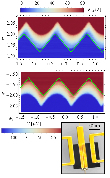
Figure 6: (color online) SQUID voltage as a function of control parameters used to extract its parameters in the absence of split-coil magnetic field. The bias current axis is normalized such that $i_{B}=I_{B}/I_{0}$, where $I_{0}=317.5{\rm\mu A}$. The extracted values, using the calculated $i_{c\pm}(\phi_{a})$ curves (green lines), are $\beta_{L}=21.1$ and $\alpha_{I}=-0.027$, corresponding to $L=69{\rm pH}$, which is consistent with the value calculated using 3D-MLSI Khapaev et al. (2001). Note the absence of a sharp cusp. The voltage is truncated at higher currents due to voltage compliance settings. Inset: A false-color optical micrograph of the device.

A.2 Mechanical parameters

Each of the doubly-clamped beams has length $\ell=100{\rm\mu m}$, lateral width $w=14{\rm\mu m}$, thickness $t={\rm 0.7\mu m}$ and bare mass $m=8.7{\rm ng}$, with $m_{{\rm eff}}=0.735m$ Ekinci et al. (2004). The mode frequencies of the beams were characterized at zero magnetic field, and only the lowest frequency mode was actuated. The mode profile (measured by scanning the position of the optical fiber) indicated that only one of the beams vibrated with this frequency, and that the second beam had a much higher fundamental flexural mode of $f_{1}=673.5{\rm KHz}$, so that intermode coupling could be safely disregarded.

A.3 Coupling constant

In this section we discuss the coupling constant $g=\lambda\ell B\sqrt{I_{0}/m_{{\rm eff}}\Phi_{0}}$ between the SQUID and the beam. Here, $\lambda$ is a geometric correction factor which includes corrections due to mechanical mode shape, effective mass mode and magnetic field screening. To extract $\lambda$ from the measurements, we use the fact that for $i_{B}<i_{c,{\mathrm{min}}}$, the Lorentz force acting on the beam is nearly linear in $u$ for almost all values of $\phi_{a}$(see Fig. 4). This translates to a nearly constant shift of the frequency of the mechanical mode, which we can use to fit $\lambda$. From this we obtain $\lambda=0.6$.

A.4 Detection and actuation

Capacitive actuation and detection of the mechanical mode are both accomplished using the Niobium coated optical fiber, which is connected galvanically to the output of a sweeping function generator. The function generator also provides a reference signal to an RF lock in amplifier (LIA). Since the SQUID is top-coated with gold, it is highly reflective, and forms one side of an optical cavity. The other side of the cavity is formed at the dielectric interface between the tip of the fiber and free space. The power reflected from this optical cavity is converted to voltage by an RF photodetector, and fed to the input of the LIA. In this manner, the LIA functions as a network analyzer with the capability to sweep the driving frequency both in the up and down directions. This two-sided sweep is required in order to characterize the bistable regions in the frequency response of the beam.

Appendix B Modeling the SQUID-beam interaction

The normalized equations of motion for a symmetric SQUID in the RCSJ model and the amplitude of the driven mode in the harmonic approximation are

$$\beta_{c}\omega_{c}^{-2}\ddot{\gamma}+\omega_{c}^{-1}\dot{\gamma}+2\cos\left(\frac{\gamma_{-}}{2}\right)\sin\left(\frac{\gamma}{2}\right) = i_{B}+i_{N,+}$$ (5a)

$$\beta_{c}\omega_{c}^{-2}\ddot{\gamma}_{-}+\omega_{c}^{-1}\dot{\gamma}_{-}+2\cos\left(\frac{\gamma}{2}\right)\sin\left(\frac{\gamma_{-}}{2}\right) = -2j+i_{N,-}$$ (5b)

$$\frac{\gamma_{-}}{2\pi}-\phi_{a}-u = \frac{1}{2}\beta_{L}j$$ (5c)

$$\ddot{u}+Q_{m}^{-1}\omega_{0}\dot{u}+\omega_{0}^{2}u = g^{2}\left(\frac{1}{2}i_{B}+j\right)+h_{d}\cos(\omega_{p}t),$$ (5d)

where $\gamma_{-}=\gamma_{2}-\gamma_{1}$, $i_{N,\pm}=I_{N,\pm}/I_{0}$, and $I_{N,\pm}$ is current noise in the junctions. The response of the driven mode to the excitation by the SQUID was obtained by calculating $j_{\mathrm{av}}$, as defined in the body of the text, for the range $0<i_{B}<3$, $0<\phi_{a}<1$ of the control parameters. When the SQUID was in the S-state, $j_{\mathrm{av}}$ was obtained by finding all roots of Eq. (5a-5c) in the steady state. In general, more than one such root (or well of the SQUID potential) exists when $\beta_{L}>0$. However, this multiplicity comes into effect only near values of $\phi_{a}$ for which a well disappears (see theoretical panel in Fig. 4), which are the points near which discrepancy between the model and the experiment exists. In the R-state, $j_{\mathrm{av}}$ was found by integrating $j(t)$ which was numerically computed using Eq. (5a-5c) over a single period $\Theta$. The asymmetry was found to be small in our device ($\alpha_{I}=-0.027$), and therefore was not taken into account in the numerical calculations.

After $j_{\mathrm{av}}(\phi_{a},i_{B})$ was obtained, the derivatives $\partial j_{\mathrm{av}}/\partial\phi_{a}$, $\partial^{3}j_{\mathrm{av}}/\partial\phi_{a}^{3}$ were calculated numerically. These were used to obtain the frequency shift and Duffing coefficient for the equation of the mode amplitude in the rotating wave approximation Landau and Lifshitz (1976); Lifshitz and M. C. Cross (2008)

$$\left[\left(\delta+\frac{1}{2}\epsilon d_{1}+\frac{3}{8}\epsilon d_{3}|A|^{2}\right)^{2}+\left(\frac{1}{2Q_{m}}\right)^{2}\right]|A|^{2}=\frac{1}{4}\epsilon_{d}^{2},$$ (6)

where $\delta=(\omega_{p}-\omega_{0})/\omega_{0}$, $d_{1}=\frac{1}{2}\partial j_{\mathrm{av}}/\partial\phi_{a}$, $d_{3}=\frac{1}{6}\partial^{3}j_{\mathrm{av}}/\partial\phi_{a}^{3}$, $\epsilon_{d}=h_{d}/\omega_{0}^{2}$, $\epsilon=g^{2}/\omega_{0}^{2}$, and $u(t)=\frac{1}{2}Ae^{-i(1+\delta)\omega_{0}t}+{\rm c.c}$. This was used to generate the theoretical panels in Figs. 2, 3 and 4.

Appendix C Analytical expression for $j_{\mathrm{av}}$ near the bifurcation cusp point

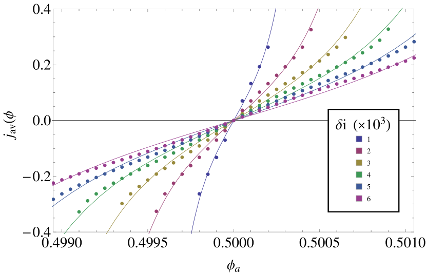
Figure 7: (color online) A comparison of the analytical expansion Eq. (12) and the value of $j_{{\rm av}}(\delta\phi)$ obtained by numerically integrating the equations of motion (5), with $\beta_{L}=0.1$, $\beta_{c}=0.05$, no noise and $u=0$.

Following the main text, we expand the potential Eq. (2) around the points $\gamma_{c\pm}$ defined by $v^{\prime\prime}(\gamma_{c\pm})=0$ and $v^{\prime\prime\prime}(\gamma_{c\pm})<0$. Two such points exist for a single period of $v(\gamma)+i_{B}\gamma$, and we find that near them the equation of motion for $\gamma$ can be written as

$$\frac{{\rm d}\gamma}{{\rm d}\tau}=\delta i+c_{0\pm}+c_{2\pm}(\gamma-\gamma_{c\pm})^{2}+\dots,$$ (7)

where

$$c_{0\pm}(\delta\phi) =\frac{\pi}{2}\beta_{L}\mp 2\pi\left(\delta\phi+\frac{1}{2}\beta_{L}j_{c\pm}\right)\sqrt{1-j_{c\pm}^{2}},$$ (8a)

$$c_{2\pm}(\delta\phi) =\pm\frac{\pi}{4}\left(\delta\phi+2\beta_{L}j_{c\pm}\right)\sqrt{1-j_{c\pm}^{2}},$$ (8b)

and

$$j_{c\pm}(\delta\phi)=\pm\sqrt{\frac{1}{2}+\left(\frac{\delta\phi}{2\beta_{L}}\right)^{2}}-\frac{\delta\phi}{2\beta_{L}}.$$ (9)

The solution of Eq. (7) truncated after the quadratic term is $\gamma_{\pm}(\tau)=\gamma_{c\pm}+\eta_{\pm}\tan\left(\pi\frac{\tau}{\tau_{\pm}}\right)$, where $\eta_{\pm}$ and $\tau_{\pm}$ are given by

$$\tau_{\pm}=\frac{\pi}{\sqrt{\left(\delta i+c_{0\pm}\right)c_{2\pm}}}$$ (10)

and

$$\eta_{\pm}=\sqrt{\frac{\delta i+c_{0\pm}}{c_{2\pm}}}.$$ (11)

Since for $\delta\phi=0$ we have $j_{c\pm}=\pm 1/\sqrt{2}$ and therefore $c_{0\pm}=0$, we see that the time spent near the slow points indeed scales as $(\delta i)^{-\frac{1}{2}}$, as expected from an infinite period bifurcation Strogatz (2001). We can now calculate $j_{\mathrm{av}}$ using these solutions and the fact that $j(\tau)=-\cos\left(\gamma/2\right)$, and we obtain

$$j_{\mathrm{av}} =\frac{1}{\Theta}\int_{0}^{\Theta}j(\tau){\rm d}\tau=\frac{j_{c+}\tau_{+}e^{-\frac{1}{2}\eta_{+}}+j_{c-}\tau_{-}e^{-\frac{1}{2}\eta_{-}}}{\tau_{+}+\tau_{-}}$$

$$+O(\sqrt{\delta i}).$$ (12)

A comparison between $j_{\mathrm{av}}$ obtained with this approximation and the one calculated numerically using the equations of motion Eq. (5a-5c) is found in Fig. 7.