Finite temperature fermionic condensate and currents
in topologically nontrivial spaces

Abstract

We investigate the finite temperature fermionic condensate and the expectation values of the charge and current densities for a massive fermion field in a spacetime background with an arbitrary number of toroidally compactified spatial dimensions in the presence of a non-vanishing chemical potential. Periodicity conditions along compact dimensions are taken with arbitrary phases and the presence of a constant gauge field is assumed. The latter gives rise to Aharonov-Bohm-like effects on the expectation values. They are periodic functions of magnetic fluxes enclosed by compact dimensions with the period equal to the flux quantum. The current density has nonzero components along compact dimensions only. Both low- and high-temperature asymptotics of the expectation values are studied. In particular, it has been shown that at high temperatures the current density is exponentially suppressed. This behavior is in sharp contrast with the corresponding asymptotic in the case of a scalar field, where the current density linearly grows with the temperature. The features for the models in odd dimensional spacetimes are discussed. Applications are given to cylindrical and toroidal nanotubes described within the framework of effective Dirac theory for the electronic subsystem.

PACS numbers: 03.70.+k, 11.10.Kk, 03.75.Hh, 61.46.Fg

1 Introduction

There exists a variety of different models in which the physical problem is formulated in spacetime backgrounds having compact spatial dimensions. In high energy physics, the well-known examples are Kaluza-Klein type models, supergravity and superstring theories. The models with a compact universe may play an important role in providing proper initial conditions for inflation [1] (for physical motivations of considering compact universes see also Ref. [2]). An interesting application of the field theoretical models having compact dimensions recently appeared in condensed matter physics. The long-wavelength description of the electronic states in graphene can be formulated in terms of an effective Dirac theory in a two-dimensional space with the Fermi velocity playing the role of the speed of light (for a review see Ref. [3]). Carbon nanotubes are generated by rolling up a graphene sheet to form a cylinder, and the background space for the corresponding Dirac-like theory has the topology $R^{1}\times S^{1}$. The compactification along the nanotube axis gives rise to another class of graphene-made structures called toroidal carbon nanotubes having the topology of a two-torus.

In field-theoretical models formulated on a spacetime background with compact dimensions, the periodicity conditions imposed on fields separate configurations with suitable wavelengths. This leads to the shift in the expectation values of various physical observables in quantum field theory. In particular, many authors have investigated the vacuum energy and stresses induced by the presence of compact dimensions (for reviews see Refs. [4], [5]). This effect, known as topological Casimir effect, is a physical example of the connection between global properties of spacetime and quantum phenomena. In higher-dimensional field theories with compact extra dimensions, the Casimir energy induces an effective potential providing a stabilization mechanism for moduli fields and thereby fixing the effective gauge couplings. The Casimir effect has also been considered as an origin for the dark energy in Kaluza-Klein type models and in braneworlds [6].

The effects of the toroidal compactification of spatial dimensions on the properties of quantum vacuum for various spin fields have been discussed by several authors (see, for instance, Refs. [4]-[8], and references therein). One-loop quantum effects in de Sitter spacetime with toroidally compact dimensions are studied in Refs. [9] and [10] for scalar and fermionic fields, respectively. The main part of the papers, devoted to the influence of the nontrivial topology on the properties of the quantum vacuum, considers the vacuum energy and stresses. These quantities are chosen because of their close connection with the structure of spacetime through the general theory of gravity. Another important characteristic for charged fields is the expectation value of the current density. In Ref. [11], we have investigated the vacuum expectation value of the current density for a fermionic field in spaces with an arbitrary number of toroidally compactified dimensions. Application of the general results were given to the electrons of a graphene sheet rolled into cylindrical and toroidal shapes. Combined effects of compact spatial dimensions and boundaries on the vacuum expectation values of the fermionic current have been discussed recently in Ref. [12]. The geometry of boundaries is given by two parallel plates on which the fermion field obeys bag boundary conditions. Vacuum expectation values of the current densities for charged scalar and Dirac spinor fields in de Sitter spacetime with toroidally compact spatial dimensions are investigated in Ref. [13]. The effects of nontrivial topology around a conical defect on the current induced by a magnetic flux were discussed in Ref. [14] for scalar and fermion fields.

The finite temperature effects are of key importance in both types of models with compact dimensions used in the cosmology of the early Universe and in condensed matter physics. In Ref. [15], we have investigated the finite temperature expectation values of the charge and current densities for a complex scalar field with nonzero chemical potential in the background of a flat spacetime with spatial topology $R^{p}\times(S^{1})^{q}$. In the latter, the separate contributions to the charge and current densities coming from the Bose-Einstein condensate and from excited states were studied. Continuing in this line of investigations, in the present paper we consider the effects of toroidal compactification of spatial dimensions on the finite temperature fermionic condensate, charge and current densities for a massive field in the presence of a non-vanishing chemical potential. The thermal Casimir effect in cosmological models with nontrivial topology has been discussed in Refs. [16]. A general discussion of the finite temperature effects for a scalar field in higher dimensional product manifolds with compact subspaces is given in Ref. [17]. Specific calculations are presented for the cases with the internal space being a torus or a sphere. In Ref. [18], the corresponding results are extended to the case with a nonzero chemical potential. In the previous discussions about the effects from nontrivial topology and finite temperature, the authors mainly consider periodicity and antiperiodicity conditions imposed on the fields along compact dimensions. The latter correspond to untwisted and twisted configurations of fields respectively. In this case the current density corresponding to a conserved charge associated with an internal symmetry vanishes. As it will be seen below, the presence of a constant gauge field, interacting with a charged quantum field, will induce a nontrivial phase in the periodicity conditions along compact dimensions. As a consequence of this, nonzero components of the current density appear along compact dimensions. This is a sort of Aharonov-Bohm-like effect related to the nontrivial topology of the background space.

In what follows we consider the fermionic condensate and the expectation values of the charge and current densities in $(D+1)$-dimensional spacetime with spatial topology $R^{p}\times(S^{1})^{q}$ (with $p+q=D$). The corresponding results can be used in three types of models. For the first one we have $p=3$, $q>1$, and it corresponds to the universe with Kaluza-Klein-type extra dimensions. In these models, the currents along compact dimensions are sources of cosmological magnetic fields. In the second class of models $D=3$, and the results given below describe how the properties of the universe are changed by one-loop quantum effects induced by the compactness of spatial dimensions. Another possible range for the applications of the results obtained in the present paper could be graphene-made structures like cylindrical and toroidal carbon nanotubes described within the framework of Dirac-like theory.

The paper is organized as follows. In the next section we describe the geometry of the problem under consideration and present a complete set of mode functions needed in the evaluation of expectation values. Then, the fermionic condensate is investigated for a complex fermionic field in thermal equilibrium. In Sections 3 and 4, the expectation values of the charge and current densities are considered. Several representations are provided and the asymptotic behaviors are investigated in various limiting cases, including low- and high-temperature limits. The features of the model in odd spacetime dimensions are discussed in Section 5. Applications of general results to a $(2+1)$-dimensional model describing the long-wavelength excitations of the electronic subsystem in a graphene sheet are given in Section 6. The main results are summarized in Section 7. Throughout the paper, except in Section 6, we use the units $\hbar=c=1$.

2 Fermionic condensate

Let us consider a fermionic field $\psi$ on a background of $(D+1)$-dimensional flat spacetime having the spatial topology $R^{p}\times(S^{1})^{q}$, $p+q=D$. We shall denote by $\mathbf{z}=(\mathbf{z}_{p},\mathbf{z}_{q})$ the Cartesian coordinates, where $\mathbf{z}_{p}=(z^{1},\ldots,z^{p})$ and $\mathbf{z}_{q}=(z^{p+1},\ldots,z^{D})$ correspond to uncompactified and compactified dimensions, respectively. One has $-\infty<z^{l}<\infty$ for $l=1,\ldots,p$, and $0\leqslant z^{l}\leqslant L_{l}$ for $l=p+1,\ldots,D$, with $L_{l}$ being the length of the $l$th compact dimension. In the presence of an external gauge field $A_{\mu}$, the evolution of the field is described by the Dirac equation

$$i\gamma^{\mu}D_{\mu}\psi-m\psi=0\ ,\;D_{\mu}=\partial_{\mu}+ieA_{\mu}.$$ (2.1)

For the irreducible representation of the Clifford algebra the Dirac matrices $\gamma^{\mu}$ are $N\times N$ matrices with $N=2^{[(D+1)/2]}$ (the square brackets mean the integer part of the enclosed expression). We take these matrices in the Dirac representation:

$$\gamma^{0}=\left(\begin{array}[]{cc}1&0\\ 0&-1\end{array}\right),\;\gamma^{\mu}=\left(\begin{array}[]{cc}0&\sigma_{\mu}\\ -\sigma_{\mu}^{+}&0\end{array}\right),\;\mu=1,2,\ldots,D.$$ (2.2)

From the anticommutation relations for the Dirac matrices we get $\sigma_{\mu}\sigma_{\nu}^{+}+\sigma_{\nu}\sigma_{\mu}^{+}=2\delta_{\mu\nu}$. In the case $D=2$ one has $N=2$ and the Dirac matrices can be taken in the form $\gamma^{\mu}=(\sigma_{\mathrm{P}3},i\sigma_{\mathrm{P}2},-i\sigma_{\mathrm{P}1})$, with $\sigma_{\mathrm{P}\mu}$ being the usual $2\times 2$ Pauli matrices . In what follows we assume that $A_{\mu}=(A_{0},-\mathbf{A})$ is a constant vector potential. Although the corresponding magnetic field strength vanishes, the non-trivial topology of the background spacetime induces Aharonov-Bohm-like effects for expectation values of physical observables. As it will be seen below, the fermionic condensate (FC) and the current density are periodic functions of the components of the gauge field along compact dimensions.

One of the characteristic features of field theory on backgrounds with nontrivial topology is the appearance of topologically inequivalent field configurations and, in addition to the field equation (2.1), we need to specify the periodicity conditions obeyed by the field operator along compact dimensions. Here we consider the generic quasiperiodicity boundary conditions,

$$\psi(t,\mathbf{z}_{p},\mathbf{z}_{q}+L_{l}\mathbf{e}_{l})=e^{2\pi i\alpha_{l}}\psi(t,\mathbf{z}_{p},\mathbf{z}_{q}),$$ (2.3)

with constant phases $\alpha_{l}$ and with $\mathbf{e}_{l}$ being the unit vector along the direction of the coordinate $z^{l}$, $l=p+1,\ldots,D$. Twisted and untwisted periodicity conditions, most often discussed in the literature, correspond to special cases $\alpha_{l}=1/2$ and $\alpha_{l}=0$, respectively. As it will be discussed below, for a Dirac field describing the long-wavelength properties of graphene, the cases $\alpha_{l}=0,\pm 1/3$ are realized in carbon nanotubes.

Here, we are interested in the effects of non-trivial topology and the magnetic fluxes enclosed by compact dimensions on the FC and the expectation values of the charge and current densities assuming that the field is in thermal equilibrium at finite temperature $T$. Firstly, we consider the FC defined as

$$\left\langle\bar{\psi}\psi\right\rangle=\mathrm{tr}[\widehat{\rho}\bar{\psi}\psi],$$ (2.4)

where $\bar{\psi}=\psi^{+}\gamma^{0}$ is the Dirac conjugated spinor, $\hat{\rho}$ is the density matrix and $\left\langle\cdots\right\rangle$ means the ensemble average. For the thermodynamical equilibrium distribution at temperature $T$, the density matrix has the standard form:

$$\hat{\rho}=Z^{-1}e^{-\beta(\hat{H}-\mu^{\prime}\hat{Q})},\;\beta=1/T,$$ (2.5)

where $\hat{H}$ is the Hamilton operator, $\widehat{Q}$ denotes a conserved charge and $\mu^{\prime}$ is the related chemical potential. The grand-canonical partition function $Z$ is defined as:

$$Z=\mathrm{tr}[e^{-\beta(\hat{H}-\mu^{\prime}\hat{Q})}].$$ (2.6)

For the evaluation of the expectation value in Eq. (2.4) we shall employ the direct mode summation technique. Let $\{\psi_{\sigma}^{(+)},\psi_{\sigma}^{(-)}\}$ be a complete set of normalized positive- and negative-energy solutions of Eq. (2.1) obeying the quasiperiodicity conditions (2.3). The corresponding energies will be denoted by $\varepsilon_{\sigma}^{(\pm)}$. Here $\sigma$ stands for a set of quantum numbers specifying the solutions. For the evaluation of the FC we expand the field operator as:

$$\psi=\sum_{\sigma}[\hat{a}_{\sigma}\psi_{\sigma}^{(+)}+\hat{b}_{\sigma}^{+}\psi_{\sigma}^{(-)}],$$ (2.7)

and use the relations

$$\mathrm{tr}[\hat{\rho}\hat{a}_{\sigma}^{+}\hat{a}_{\sigma^{\prime}}] = \frac{\delta_{\sigma\sigma^{\prime}}}{e^{\beta(\varepsilon_{\sigma}^{(+)}-\tilde{\mu})}+1},$$

$$\mathrm{tr}[\hat{\rho}\hat{b}_{\sigma}^{+}\hat{b}_{\sigma^{\prime}}] = \frac{\delta_{\sigma\sigma^{\prime}}}{e^{\beta(\varepsilon_{\sigma}^{(-)}+\tilde{\mu})}+1},$$ (2.8)

with $\tilde{\mu}=e\mu^{\prime}$. In Eq. (2.8), $\delta_{\sigma\sigma^{\prime}}$ corresponds to the Kronecker delta for the discrete components of the collective index $\sigma$ and to the Dirac delta function for the continuous ones. The expressions for $\mathrm{tr}[\hat{\rho}\hat{a}_{\sigma^{\prime}}\hat{a}_{\sigma}^{+}]$ and $\mathrm{tr}[\hat{\rho}\hat{b}_{\sigma^{\prime}}\hat{b}_{\sigma}^{+}]$ are obtained from (2.8) by using the anticommutation relations for the creation and annihilation operators.

Substituting the expansion (2.7) into Eq. (2.4) and using the relations (2.8), for the FC we get the following expression:

$$\left\langle\bar{\psi}\psi\right\rangle=\left\langle\bar{\psi}\psi\right\rangle_{0}+\sum_{\sigma}\sum_{j=+,-}\frac{j\bar{\psi}_{\sigma}^{(j)}\psi_{\sigma}^{(j)}}{e^{\beta(\varepsilon_{\sigma}^{(j)}-j\tilde{\mu})}+1},$$ (2.9)

where

$$\left\langle\bar{\psi}\psi\right\rangle_{0}=\sum_{\sigma}\bar{\psi}_{\sigma}^{(-)}\psi_{\sigma}^{(-)},$$ (2.10)

is the vacuum expectation value of the FC. The latter was investigated in Ref. [8] and here we will be mainly concerned with the finite temperature effects provided by the second term in the right-hand side of Eq. (2.9). For the evaluation of the FC we need to specify the mode-functions. In accordance with the symmetry of the problem, we take these functions in the form of plane waves:

$$\psi_{\sigma}^{(+)} = A_{\sigma}^{(+)}e^{i\mathbf{k}\cdot\mathbf{z}-i\varepsilon_{\mathbf{k}}^{(+)}t}\left(\begin{array}[]{c}w_{\chi}^{(+)}\\ \frac{(\mathbf{k}-e\mathbf{A})\cdot\boldsymbol{\sigma}^{+}}{\varepsilon_{\mathbf{k}}^{(+)}-eA_{0}+m}w_{\chi}^{(+)}\end{array}\right),$$ (2.13)

$$\psi_{\sigma}^{(-)} = A_{\sigma}^{(-)}e^{i\mathbf{k}\cdot\mathbf{z}+i\varepsilon_{\mathbf{k}}^{(-)}t}\left(\begin{array}[]{c}-\frac{(\mathbf{k}-e\mathbf{A})\cdot\boldsymbol{\sigma}}{\varepsilon_{\mathbf{k}}^{(-)}+eA_{0}+m}w_{\chi}^{(-)}\\ w_{\chi}^{(-)}\end{array}\right),$$ (2.16)

where $\boldsymbol{\sigma}=(\sigma_{1},\sigma_{2},\ldots,\sigma_{D})$ and

$$\varepsilon_{\mathbf{k}}^{(\pm)}=\varepsilon_{\sigma}^{(\pm)}=\pm eA_{0}+\sqrt{\left(\mathbf{k}-e\mathbf{A}\right)^{2}+m^{2}}.$$ (2.17)

In Eq. (2.16), $w_{\chi}^{(\pm)}$, $\chi=1,\ldots,N/2$, are one-column matrices having $N/2$ rows with the elements $w_{\chi l}^{(\pm)}=\delta_{\chi l}$.

For the components of the momentum $\mathbf{k}$ along uncompactified dimensions one has $-\infty<k_{l}<\infty$, $l=1,\ldots,p$. The components along compact dimensions are quantized by the quasiperiodicity conditions (2.3) and the corresponding eigenvalues are given by

$$k_{l}=2\pi(n_{l}+\alpha_{l})/L_{l},\;n_{l}=0,\pm 1,\pm 2,\ldots,$$ (2.18)

with $l=p+1,\ldots,D$. The coefficients $A_{\sigma}^{(\pm)}$ in Eq. (2.16) are determined by the orthonormalization condition $\int d^{D}x\,\psi_{\sigma}^{(\lambda)+}\psi_{\sigma^{\prime}}^{(\lambda^{\prime})}=\delta_{\sigma\sigma^{\prime}}\delta_{\lambda\lambda^{\prime}}$ with $\lambda,\lambda^{\prime}=+,-$. This gives:

$$A_{\sigma}^{(\pm)2}=\frac{\varepsilon_{\mathbf{k}}^{(\pm)}\mp eA_{0}+m}{2(2\pi)^{p}V_{q}(\varepsilon_{\mathbf{k}}^{(\pm)}\mp eA_{0})},$$ (2.19)

where $V_{q}=L_{p+1}\cdots L_{D}$ is the volume of the compact subspace. Now the set of quantum numbers is specified to $\sigma=(\mathbf{k}_{p},\mathbf{n}_{q},\chi)$, where $\mathbf{k}_{p}=(k_{1},\ldots,k_{p})$, $\mathbf{n}_{q}=(n_{p+1},\ldots,n_{D})$, and

$$\sum_{\sigma}=\int d\mathbf{k}_{p}\sum_{\mathbf{n}_{q}\in\mathbf{Z}^{q}}\sum_{\chi=1}^{N/2}.$$ (2.20)

Substituting the mode functions (2.16) into Eq. (2.9) and shifting the integration variable $\mathbf{k}_{p}\rightarrow\mathbf{k}_{p}+e\mathbf{A}_{p}$, we find the following expression:

$$\left\langle\bar{\psi}\psi\right\rangle=\left\langle\bar{\psi}\psi\right\rangle_{0}+\sum_{j=+,-}\left\langle\bar{\psi}\psi\right\rangle_{j},$$ (2.21)

where

$$\left\langle\bar{\psi}\psi\right\rangle_{\pm}=\frac{Nm}{2(2\pi)^{p}V_{q}}\int d\mathbf{k}_{p}\sum_{\mathbf{n}_{q}\in\mathbf{Z}^{q}}\frac{1/\varepsilon(\mathbf{k})}{e^{\beta(\varepsilon(\mathbf{k})\mp\mu)}+1},$$ (2.22)

is the part in the FC coming from particles (upper sign) and antiparticles (lower sign). In Eq. (2.22), $\mu=\tilde{\mu}-eA_{0}$,

$$\varepsilon(\mathbf{k})=\sqrt{\mathbf{k}_{p}^{2}+\varepsilon_{\mathbf{n}_{q}}^{2}},\;\varepsilon_{\mathbf{n}_{q}}=\sqrt{\sum\nolimits_{l=p+1}^{D}\tilde{k}_{l}^{2}+m^{2}},$$ (2.23)

and we have introduced the notations

$$\tilde{k}_{l}=2\pi(n_{l}+\tilde{\alpha}_{l})/L_{l},\;\tilde{\alpha}_{l}=\alpha_{l}-eL_{l}\mathbf{A}_{l}/2\pi.$$ (2.24)

As it is seen, the FC does not depend on the components of the vector potential along non compact dimensions.

The dependence on the phases $\alpha_{l}$ and on the components of the vector potential along compact dimensions enters in the form of the combination $\tilde{\alpha}_{l}$ in Eq. (2.24). We could see this directly by the gauge  transformation $A_{\mu}=A_{\mu}^{\prime}+\partial_{\mu}\Lambda(x)$, $\psi(x)=\psi^{\prime}(x)e^{-ie\Lambda(x)}$, with $\Lambda(x)=A_{\mu}z^{\mu}$. The new function $\psi^{\prime}(x)$ obeys the Dirac equation with $A_{\mu}^{\prime}=0$ and the periodicity condition $\psi^{\prime}(t,\mathbf{z}_{p},\mathbf{z}_{q}+L_{l}\mathbf{e}_{l})=e^{2\pi i\tilde{\alpha}_{l}}\psi^{\prime}(t,\mathbf{z}_{p},\mathbf{z}_{q})$. The expectation values are not changed under the gauge transformation and, in the new gauge, the parameter $\tilde{\alpha}_{l}$ appears, instead of $\alpha_{l}$ and $\mathbf{A}_{l}$. Note that we can write $eL_{l}\mathbf{A}_{l}/2\pi=\phi_{l}/\phi_{0}$, where $\phi_{l}$ is the magnetic flux enclosed by the $l$th compact dimensions and $\phi_{0}=2\pi/e$ is the flux quantum. Hence, the presence of a constant gauge field is equivalent to the shift of the phases in the periodicity conditions along compact dimensions. In particular, a nontrivial phase is induced for the special cases of twisted and untwisted fermionic fields. As it will be discussed below, this leads to the appearance of the nonzero current density along compact dimensions. Another interesting physical effect of a constant gauge field is the topological generation of a gauge field mass by the toroidal spacetime (see Ref. [19] and references therein).

If we present the phases $\tilde{\alpha}_{l}$ in the form $\tilde{\alpha}_{l}=\tilde{\alpha}_{l}^{(f)}+\tilde{\alpha}_{l}^{(i)}$, with $\tilde{\alpha}_{l}^{(i)}$ being an integer and $|\tilde{\alpha}_{l}^{(f)}|\leqslant 1/2$, then, as it is seen from Eq. (2.22), the FC depends on the fractional part $\tilde{\alpha}_{l}^{(f)}$ only. We will denote by $\varepsilon_{0}$ the smallest value of the energy $\varepsilon(\mathbf{k})$:

$$\varepsilon_{0}=\sqrt{\sum\nolimits_{l=p+1}^{D}(2\pi\tilde{\alpha}_{l}^{(f)}/L_{l})^{2}+m^{2}},$$ (2.25)

which corresponds to $n_{l}=-\tilde{\alpha}_{l}^{(i)}$. Note that, while the bosonic chemical potential is restricted by $|\mu|\leqslant$ $\varepsilon_{0}$, the fermionic chemical potential can have any value with respect to $\varepsilon_{0}$.

Firstly, we consider the case $|\mu|<$ $\varepsilon_{0}$. With this assumption, by making use of the expansion

$$(e^{y}+1)^{-1}=-\sum_{n=1}^{\infty}(-1)^{n}e^{-ny}\ ,$$ (2.26)

after the integration over $\mathbf{k}_{p}$, from (2.22) we get

$$\left\langle\bar{\psi}\psi\right\rangle_{\pm}=-\frac{Nm}{(2\pi)^{(p+1)/2}V_{q}}\sum_{n=1}^{\infty}(-1)^{n}e^{\pm n\beta\mu}\sum_{\mathbf{n}_{q}\in\mathbf{Z}^{q}}\varepsilon_{\mathbf{n}_{q}}^{p-1}f_{(p-1)/2}(n\beta\varepsilon_{\mathbf{n}_{q}}).$$ (2.27)

In (2.27) and in what follows we use the notation

$$f_{\nu}(x)=K_{\nu}(x)/x^{\nu},$$ (2.28)

with $K_{\nu}(x)$ being the Macdonald function. Combining Eqs. (2.21) and (2.27), for the total FC one finds:

$$\left\langle\bar{\psi}\psi\right\rangle=\left\langle\bar{\psi}\psi\right\rangle_{0}-\frac{2Nm}{(2\pi)^{(p+1)/2}V_{q}}\sum_{n=1}^{\infty}(-1)^{n}\cosh(n\beta\mu)\sum_{\mathbf{n}_{q}\in\mathbf{Z}^{q}}\varepsilon_{\mathbf{n}_{q}}^{p-1}f_{(p-1)/2}(n\beta\varepsilon_{\mathbf{n}_{q}}).$$ (2.29)

As it is seen from the above equation, the FC is a periodic function of $\tilde{\alpha}_{l}$ with the period equal to unity. In particular, FC is a periodic function of the flux enclosed by a compact dimension with the period equal to the flux quantum.

Let us consider the behavior of the FC, given by Eq. (2.29), in the asymptotic regions of the parameters. If the lengths of the compact dimensions are large, $L_{l}\gg\beta,m$, the dominant contribution comes from large values of $|n_{l}|$, and we can replace the summation by the integration, $\sum_{\mathbf{n}_{q}\in\mathbf{Z}^{q}}\rightarrow V_{q}(2\pi)^{-q}\int d\mathbf{k}_{q}$ with $\varepsilon_{\mathbf{n}_{q}}=\sqrt{\mathbf{k}_{q}^{2}+m^{2}}$. The integral is evaluated by using the formula

$$\int d^{r}\mathbf{x}\,(\mathbf{x}^{2}+a^{2})^{\nu}f_{\nu}(b\sqrt{\mathbf{x}^{2}+a^{2}})=(2\pi)^{r/2}a^{2\nu+r}f_{\nu+r/2}(ab),$$ (2.30)

and, to the leading order, we obtain the FC in topologically trivial Minkowski spacetime:

$$\left\langle\bar{\psi}\psi\right\rangle_{\mathrm{M}}=-\frac{2Nm^{D}}{(2\pi)^{(D+1)/2}}\sum_{n=1}^{\infty}(-1)^{n}\cosh(n\beta\mu)f_{(D-1)/2}(mn\beta).$$ (2.31)

Here we have renormalized the zero temperature FC in Minkowski spacetime to zero. More precisely, if for a part of compact dimensions (with the index $r$) the lengths are large, by replacing the corresponding series by the integrations and using (2.30), it is seen from Eq. (2.29) that the result obtained is equivalent to that for the topology $R^{p+r}\times(S^{1})^{q-r}$.

In the opposite limit, when the length of the $l$th compact dimension is small compared with the other length scales and $L_{l}\ll\beta$, under the assumption $|\tilde{\alpha}_{l}|<1/2$, the dominant contribution to the series over $n_{l}$ in Eq. (2.29) comes from the term $n_{l}=0$. It can be seen that for $\tilde{\alpha}_{l}=0$, in the leading order, $L_{l}\left\langle\bar{\psi}\psi\right\rangle$ coincides with $N\left\langle\bar{\psi}\psi\right\rangle_{(p,q-1)}/N_{D-1}$, where $\left\langle\bar{\psi}\psi\right\rangle_{(p,q-1)}$ is the condensate in $(D-1)$-dimensional space of topology $R^{p}\times(S^{1})^{q-1}$ with the lengths of the compact dimensions $L_{p+1}$,…,$L_{l-1}$,$L_{l+1}$,…,$L_{D}$ ($N_{D-1}$ is the corresponding number of spinor components). For $\tilde{\alpha}_{l}\neq 0$ and for small values of $L_{l}$, the argument of the Macdonald function in Eq. (2.29) is large and the FC is suppressed by the factor $e^{-2\pi|\tilde{\alpha}_{l}|\beta/L_{l}}$.

In the low-temperature limit, the parameter $\beta$ is large and the dominant contribution to the FC comes from the term $n=1$ in the series over $n$, and from the term in the series over $\mathbf{n}_{q}$ with the smallest value of $\varepsilon_{\mathbf{n}_{q}}$. In the leading order we find

$$\left\langle\bar{\psi}\psi\right\rangle\approx\left\langle\bar{\psi}\psi\right\rangle_{0}+\frac{Nm\varepsilon_{0}^{p/2-1}e^{-\beta(\varepsilon_{0}-|\mu|)}}{2(2\pi)^{p/2}V_{q}\beta^{p/2}},$$ (2.32)

with $\varepsilon_{0}$ given by Eq. (2.25).

An alternative expression for the FC can be obtained by employing the zeta function technique [20]. We write the expression (2.21) in the form

$$\left\langle\bar{\psi}\psi\right\rangle=-\frac{Nm}{(2\pi)^{p}V_{q}}\int d\mathbf{k}_{p}\sum_{\mathbf{n}_{q}\in\mathbf{Z}^{q}}\sideset{}{{}^{\prime}}{\sum}_{n=0}^{\infty}(-1)^{n}\cosh(n\beta\mu)\frac{e^{-n\beta\varepsilon(\mathbf{k})}}{\varepsilon(\mathbf{k})},$$ (2.33)

where the prime on the sign of the sum means that the term $n=0$ should be taken with the coefficient 1/2. This term corresponds to the vacuum expectation value of the FC, $\left\langle\bar{\psi}\psi\right\rangle_{0}$. Next, we use the integral representation

$$\frac{e^{-n\beta\varepsilon(\mathbf{k})}}{\varepsilon(\mathbf{k})}=\frac{2}{\sqrt{\pi}}\int_{0}^{\infty}ds\,e^{-\varepsilon^{2}(\mathbf{k})s^{2}-n^{2}\beta^{2}/4s^{2}},$$ (2.34)

and the formula

$$\sideset{}{{}^{\prime}}{\sum}_{n=0}^{\infty}(-1)^{n}\cosh(n\beta\mu)e^{-n^{2}\beta^{2}/4s^{2}}=s\frac{\sqrt{\pi}}{\beta}\sum_{n=-\infty}^{+\infty}e^{-s^{2}[2\pi(n+1/2)/\beta+i\mu]^{2}}.$$ (2.35)

The above result can be proved by making use of the Poisson summation formula. As a result, after the integration over $s$, the FC is presented as

$$\left\langle\bar{\psi}\psi\right\rangle=-Nm\zeta(1),$$ (2.36)

where we have defined the zeta function as shown below:

$$\zeta(s)=\frac{1}{V_{q}\beta}\int\frac{d\mathbf{k}_{p}}{(2\pi)^{p}}\sum_{\mathbf{n}_{q+1}\in\mathbf{Z}^{q+1}}\Big{\{}\mathbf{k}_{p}^{2}+\sum_{l=p+1}^{D+1}[2\pi(n_{l}+\tilde{\alpha}_{l})/L_{l}]^{2}+m^{2}\Big{\}}^{-s},$$ (2.37)

with $\mathbf{n}_{q+1}=(\mathbf{n}_{q},n_{D+1})$,

$$L_{D+1}=\beta,\;\tilde{\alpha}_{D+1}=\frac{1}{2}+\frac{i\beta\mu}{2\pi}.$$ (2.38)

The renormalized value for the FC is obtained by the analytical continuation of the zeta function at $s=1$. An exponentially convergent expression for the analytic continuation is obtained by integrating over $\mathbf{k}_{p}$ and then applying the generalized Chowla-Selberg formula [21]. In this way we get:

$$\zeta(s) = \frac{m^{D+1-2s}}{(4\pi)^{(D+1)/2}}\frac{\Gamma(s-(D+1)/2)}{\Gamma(s)}+\frac{2^{1-s}m^{D+1-2s}}{(2\pi)^{(D+1)/2}\Gamma(s)}$$ (2.39)

$$\times\sideset{}{{}^{\prime}}{\sum}_{\mathbf{m}_{q+1}\in\mathbf{Z}^{q+1}}\cos(2\pi\mathbf{m}_{q+1}\cdot\boldsymbol{\alpha}_{q+1})f_{(D+1)/2-s}(mg(\mathbf{L}_{q+1},\mathbf{m}_{q+1})),$$

with $\mathbf{L}_{q+1}=(L_{p+1},\ldots,L_{D+1})$, $\boldsymbol{\alpha}_{q+1}=(\tilde{\alpha}_{p+1},\ldots,\tilde{\alpha}_{D+1})$, and the prime on the summation sign means that the term $\mathbf{m}_{q+1}=0$ should be excluded from the sum. In Eq. (2.39) we have introduced the notation

$$g(\mathbf{L}_{q+1},\mathbf{m}_{q+1})=\left(\sum\nolimits_{i=p+1}^{D+1}L_{i}^{2}m_{i}^{2}\right)^{1/2}.$$ (2.40)

The contribution of the first term in the right-hand side of Eq. (2.39) gives the zero temperature FC in the topologically trivial Minkowski spacetime. This part is subtracted in the renormalization procedure. The remaining part of the zeta function is finite, at the physical point $s=1$ and for the renormalized FC one finds

$$\left\langle\bar{\psi}\psi\right\rangle=-\frac{Nm^{D}}{(2\pi)^{(D+1)/2}}\sideset{}{{}^{\prime}}{\sum}_{\mathbf{m}_{q+1}\in\mathbf{Z}^{q+1}}\cos(2\pi\mathbf{m}_{q+1}\cdot\boldsymbol{\alpha}_{q+1})f_{(D-1)/2}(mg(\mathbf{L}_{q+1},\mathbf{m}_{q+1})).$$ (2.41)

In this formula, the term $m_{D+1}=0$ corresponds to the vacuum expectation value of the FC:

$$\left\langle\bar{\psi}\psi\right\rangle_{0}=-\frac{Nm^{D}}{(2\pi)^{(D+1)/2}}\sideset{}{{}^{\prime}}{\sum}_{\mathbf{m}_{q}\in\mathbf{Z}^{q}}\cos(2\pi\mathbf{m}_{q}\cdot\boldsymbol{\alpha}_{q})f_{(D-1)/2}(mg(\mathbf{L}_{q},\mathbf{m}_{q})),$$ (2.42)

where, again, the prime means that the term with $\mathbf{m}_{q}=0$ should be excluded.

Extracting the vacuum expectation value, the renormalized FC can also be written in the form:

$$\left\langle\bar{\psi}\psi\right\rangle = \left\langle\bar{\psi}\psi\right\rangle_{0}-\frac{2Nm^{D}}{(2\pi)^{(D+1)/2}}\sum_{n=1}^{\infty}(-1)^{n}\cosh(n\beta\mu)$$ (2.43)

$$\times\sum_{\mathbf{m}_{q}\in\mathbf{Z}^{q}}\cos(2\pi\mathbf{m}_{q}\cdot\boldsymbol{\alpha}_{q})f_{(D-1)/2}(m\sqrt{g^{2}(\mathbf{L}_{q},\mathbf{m}_{q})+n^{2}\beta^{2}}),$$

with the notation

$$g(\mathbf{L}_{q},\mathbf{m}_{q})=\left(\sum\nolimits_{i=p+1}^{D}L_{i}^{2}m_{i}^{2}\right)^{1/2}.$$ (2.44)

The equivalence of two representations, given by Eqs. (2.29) and (2.43), is seen by using the formula (see, for instance, Ref. [8])

$$\sum_{\mathbf{m}_{q}\in\mathbf{Z}^{q}}\cos(2\pi\mathbf{m}_{q}\cdot\boldsymbol{\alpha}_{q})f_{\nu}(m\sqrt{g^{2}(\mathbf{L}_{q},\mathbf{m}_{q})+n^{2}\beta^{2}})=\frac{(2\pi)^{q/2}}{V_{q}m^{2\nu}}\sum_{\mathbf{n}_{q}\in\mathbf{Z}^{q}}\varepsilon_{\mathbf{n}_{q}}^{2\nu-q}f_{\nu-q/2}(n\beta\varepsilon_{\mathbf{n}_{q}}).$$ (2.45)

In order to investigate the high-temperature asymptotic of the FC, it is convenient to transform the expression (2.41). In this expression, the term with $\mathbf{m}_{q}=0$ corresponds to the FC in the topologically trivial Minkowski spacetime (see Eq. (2.31)). Separating this part from the right-hand side of Eq. (2.41), in the remaining part instead of $\cos(2\pi\mathbf{m}_{q+1}\cdot\boldsymbol{\alpha}_{q+1})$ we write $\cos(2\pi\mathbf{m}_{q}\cdot\boldsymbol{\alpha}_{q})\cos(2\pi m_{D+1}\tilde{\alpha}_{D+1})$. Next, to the series over $m_{D+1}$ we apply the formula

$$\sum_{m_{D+1}=-\infty}^{+\infty}\cos(2\pi m_{D+1}\tilde{\alpha}_{D+1})f_{\nu}(m\sqrt{\beta^{2}m_{D+1}^{2}+a^{2}})=\frac{(2\pi)^{1/2}}{\beta m^{2\nu}}$$

$$\quad\times\sum_{n=-\infty}^{+\infty}\left[(2\pi(n+\tilde{\alpha}_{D+1})/\beta)^{2}+m^{2}\right]^{\nu-1/2}f_{\nu-1/2}(a\sqrt{(2\pi(n+\tilde{\alpha}_{D+1})/\beta)^{2}+m^{2}}),$$ (2.46)

which is a special case of Eq. (2.45). This leads to the representation

$$\left\langle\bar{\psi}\psi\right\rangle = \left\langle\bar{\psi}\psi\right\rangle_{\mathrm{M}}-\frac{NmT}{(2\pi)^{D/2}}\sideset{}{{}^{\prime}}{\sum}_{\mathbf{m}_{q}\in\mathbf{Z}^{q}}\cos(2\pi\mathbf{m}_{q}\cdot\boldsymbol{\alpha}_{q})$$ (2.47)

$$\times\sum_{n=-\infty}^{+\infty}\left[(\pi\left(2n+1\right)T+i\mu)^{2}+m^{2}\right]^{D/2-1}$$

$$\times f_{D/2-1}(g(\mathbf{L}_{q},\mathbf{m}_{q})\sqrt{(\pi\left(2n+1\right)T+i\mu)^{2}+m^{2}}).$$

At high temperatures, the dominant contribution comes from the terms with $n=0$ and $n=-1$ and from the terms in the sum over $\mathbf{m}_{q}$ with the smallest value of $g(\mathbf{L}_{q},\mathbf{m}_{q})$. If $L_{\mathrm{min}}=\mathrm{min}(L_{p+1},\ldots,L_{D})$, then, to the leading order, one finds

$$\left\langle\bar{\psi}\psi\right\rangle\approx\left\langle\bar{\psi}\psi\right\rangle_{\mathrm{M}}-\frac{2Nme^{-\pi L_{\mathrm{min}}T}}{\pi(2\beta L_{\mathrm{min}})^{(D-1)/2}}\sum_{l}\cos(2\pi\tilde{\alpha}_{l}),$$ (2.48)

where the summation goes over the compact dimensions with $L_{l}=L_{\mathrm{min}}$. From Eq. (2.48) we conclude that at high temperatures the topological part in the FC is exponentially suppressed. At high temperatures, for the Minkowskian part, to the leading order, we have

$$\left\langle\bar{\psi}\psi\right\rangle_{\mathrm{M}}\approx\frac{1-2^{2-D}}{2\pi^{(D+1)/2}}\Gamma((D-1)/2)\zeta_{\mathrm{R}}(D-1)NmT^{D-1},$$ (2.49)

where $\zeta_{\mathrm{R}}(x)$ is the Riemann zeta function. For $D=2$ one gets $\left\langle\bar{\psi}\psi\right\rangle_{\mathrm{M}}\approx(2\pi)^{-1}NmT\ln 2$.

An alternative representation for the FC, containing more detailed information, can be found from Eq. (2.33) by applying to the sum over $n_{l}$, for $p+1\leqslant l\leqslant D$, the Abel-Plana summation formula in the form [8, 22]

$$\frac{2\pi}{L_{l}}\sum_{n_{l}=-\infty}^{\infty}g(\tilde{k}_{l})f(|\tilde{k}_{l}|)=\int_{0}^{\infty}dx\,[g(x)+g(-x)]f(x)+$$

$$\quad+i\int_{0}^{\infty}dx\,[f(ix)-f(-ix)]\sum_{\lambda=\pm 1}\frac{g(i\lambda x)}{e^{xL_{l}+2\lambda\pi i\tilde{\alpha}_{l}}-1},$$ (2.50)

where $\tilde{k}_{l}$ is defined by Eq. (2.24). Taking

$$g(x)=1,\;f(x)=\frac{e^{-n\beta\sqrt{x^{2}+\mathbf{k}_{p}^{2}+\varepsilon_{\mathbf{n}_{q-1}^{l}}^{2}}}}{\sqrt{x^{2}+\mathbf{k}_{p}^{2}+\varepsilon_{\mathbf{n}_{q-1}^{l}}^{2}}},$$ (2.51)

with $\mathbf{n}_{q-1}^{l}=(n_{p+1},\ldots,n_{l-1},n_{l+1},\ldots,n_{D})$, and

$$\varepsilon_{\mathbf{n}_{q-1}^{l}}=\sqrt{\varepsilon_{\mathbf{n}_{q}}^{2}-\tilde{k}_{l}^{2}},$$ (2.52)

it can be seen that the part in the FC corresponding to the first term in the right-hand side of (2.50) corresponds to the condensate for a $D$-dimensional space of topology $R^{p+1}\times(S^{1})^{q-1}$ with the lengths of the compact dimensions $L_{p+1},\ldots,L_{l-1},L_{l+1},\ldots,L_{D}$. The latter will be denoted by $\left\langle\bar{\psi}\psi\right\rangle_{p+1,q-1}$. In the part of the FC corresponding to the second term in the right-hand side of Eq. (2.50) we use the expansion

$$\sum_{\lambda=\pm 1}\frac{1}{e^{xL_{l}+2\lambda\pi i\tilde{\alpha}_{l}}-1}=2\sum_{r=1}^{\infty}e^{-xrL_{l}}\cos(2\pi r\tilde{\alpha}_{l}).$$ (2.53)

After the integrations over $x$ and $\mathbf{k}_{p}$ with the help of the formula

$$\int_{a}^{\infty}du\,\,u^{2\nu+1}(u^{2}-a^{2})^{\beta-1}f_{\nu}(cu)=2^{\beta-1}a^{2\beta+2\nu}\Gamma(\beta)f_{\nu+\beta}(ac),$$ (2.54)

we get (the prime means that the term $n=0$ should be halved)

$$\left\langle\bar{\psi}\psi\right\rangle = \left\langle\bar{\psi}\psi\right\rangle_{p+1,q-1}-\frac{4NmL_{l}}{(2\pi)^{p/2+1}V_{q}}\sideset{}{{}^{\prime}}{\sum}_{n=0}^{\infty}(-1)^{n}\cosh(n\beta\mu)$$ (2.55)

$$\times\sum_{r=1}^{\infty}\cos(2\pi r\tilde{\alpha}_{l})\sum_{\mathbf{n}_{q-1}^{l}\in\mathbf{Z}^{q-1}}\varepsilon_{\mathbf{n}_{q-1}^{l}}^{p}f_{p/2}(\varepsilon_{\mathbf{n}_{q-1}^{l}}\sqrt{r^{2}L_{l}^{2}+n^{2}\beta^{2}}),$$

where the second term in the right-hand side of Eq. (2.55) is induced by the compactification of the $l$th dimension. In the special case of a single compact dimension one has $l=D$, $\varepsilon_{\mathbf{n}_{q-1}^{l}}=m$, and from Eq. (2.55) we obtain:

$$\left\langle\bar{\psi}\psi\right\rangle = -\frac{4Nm^{D}}{(2\pi)^{(D+1)/2}}\sideset{}{{}^{\prime}}{\sum}_{n=0}^{\infty}(-1)^{n}\cosh(n\beta\mu)$$ (2.56)

$$\times\sum_{r=1}^{\infty}\cos(2\pi r\tilde{\alpha}_{D})f_{(D-1)/2}(m\sqrt{r^{2}L_{D}^{2}+n^{2}\beta^{2}}).$$

This result coincides with the corresponding one obtained from Eq. (2.43).

In the discussion above we have assumed that $|\mu|<$ $\varepsilon_{0}$. Now we consider the case $|\mu|>$ $\varepsilon_{0}$. Let us denote by $\varepsilon_{\mathbf{n}_{q}^{(0)}}$ the largest energy for which $|\mu|>$ $\varepsilon_{\mathbf{n}_{q}^{(0)}}$. From Eqs. (2.21) and (2.22), after the integration over the angular part of $\mathbf{k}_{p}$, we get

$$\left\langle\bar{\psi}\psi\right\rangle=\left\langle\bar{\psi}\psi\right\rangle_{0}+\frac{(4\pi)^{-p/2}Nm}{\Gamma(p/2)V_{q}}\sum_{j=+,-}\sum_{\mathbf{n}_{q}\in\mathbf{Z}^{q}}\int_{\varepsilon_{\mathbf{n}_{q}}}^{\infty}dx\,\frac{(x^{2}-\varepsilon_{\mathbf{n}_{q}}^{2})^{p/2-1}}{e^{\beta(x-j\mu)}+1}.$$ (2.57)

The contribution of the states with the energies $\varepsilon_{\mathbf{n}_{q}}>|\mu|$ to the FC is treated in a way similar to that described above. The FC is an even function of the chemical potential and for definiteness we assume that $\mu>0$. In this case the finite temperature part in the FC coming from the antiparticles remains the same, whereas in the part coming from the particles the spectral ranges $\varepsilon_{\mathbf{n}_{q}}\leqslant\varepsilon_{\mathbf{n}_{q}^{(0)}}$ and $\varepsilon_{\mathbf{n}_{q}}>\varepsilon_{\mathbf{n}_{q}^{(0)}}$ should be treated separately. In this way we find the following representation:

$$\left\langle\bar{\psi}\psi\right\rangle = \left\langle\bar{\psi}\psi\right\rangle_{0}+\left\langle\bar{\psi}\psi\right\rangle_{-}+\frac{(4\pi)^{-p/2}Nm}{\Gamma(p/2)V_{q}}\sum_{\varepsilon_{\mathbf{n}_{q}}\leqslant\varepsilon_{\mathbf{n}_{q}^{(0)}}}\int_{\varepsilon_{\mathbf{n}_{q}}}^{\infty}dx\,\frac{(x^{2}-\varepsilon_{\mathbf{n}_{q}}^{2})^{p/2-1}}{e^{\beta(x-\mu)}+1}$$ (2.58)

$$-\frac{Nm}{(2\pi)^{(p+1)/2}V_{q}}\sum_{n=1}^{\infty}(-1)^{n}e^{n\beta\mu}\sum_{\varepsilon_{\mathbf{n}_{q}}>\varepsilon_{\mathbf{n}_{q}^{(0)}}}\varepsilon_{\mathbf{n}_{q}}^{p-1}f_{(p-1)/2}(n\beta\varepsilon_{\mathbf{n}_{q}}),$$

where $\left\langle\bar{\psi}\psi\right\rangle_{-}$ is given by Eq. (2.27). In the limit $T\rightarrow 0$ we get

$$\left\langle\bar{\psi}\psi\right\rangle=\left\langle\bar{\psi}\psi\right\rangle_{0}+\frac{(4\pi)^{-p/2}Nm}{\Gamma(p/2)V_{q}}\sum_{\varepsilon_{\mathbf{n}_{q}}\leqslant\varepsilon_{\mathbf{n}_{q}^{(0)}}}\int_{\varepsilon_{\mathbf{n}_{q}}}^{\mu}dx\,(x^{2}-\varepsilon_{\mathbf{n}_{q}}^{2})^{p/2-1}.$$ (2.59)

The second contribution in the right-hand side comes from the particles which occupy the states with $\varepsilon_{\mathbf{n}_{q}}<\mu$. At high temperatures, the leading term coincides with that in the topologically trivial Minkowski spacetime and is given by Eq. (2.49).

3 Charge density

In this and in the following sections we shall investigate the expectation value of the fermionic current density, assuming that the field is in a thermal equilibrium at finite temperature $T$. This quantity is given by:

$$\left\langle j^{\nu}\right\rangle=e\,\mathrm{tr}[\hat{\rho}\bar{\psi}(x)\gamma^{\nu}\psi(x)].$$ (3.1)

Substituting the expansion (2.7) and using the relations (2.8), similar to Eq. (2.9), the following mode-sum formula is obtained:

$$\left\langle j^{\nu}\right\rangle=\left\langle j^{\nu}\right\rangle_{0}+e\sum_{\sigma}\sum_{j=+,-}\frac{j\bar{\psi}_{\sigma}^{(j)}\gamma^{\nu}\psi_{\sigma}^{(j)}}{e^{\beta(\varepsilon_{\sigma}^{(j)}-j\tilde{\mu})}+1},$$ (3.2)

with

$$\left\langle j^{\nu}\right\rangle_{0}=e\sum_{\beta}\bar{\psi}_{\beta}^{(-)}(x)\gamma^{\nu}\psi_{\beta}^{(-)}(x),$$ (3.3)

being the corresponding vacuum expectation value. Details of the calculations here are similar to those for the FC, and we will describe the main steps only.

Firstly, we consider the charge density corresponding to the component $\nu=0$. As it has been shown in Ref. [11], the renormalized vacuum expectation value for the charge density vanishes: $\left\langle j^{0}\right\rangle_{0,\mathrm{ren}}=0$. By taking into account Eq. (2.16), for the finite temperature part of the charge density we get

$$\left\langle j^{0}\right\rangle=\left\langle j^{0}\right\rangle_{+}+\left\langle j^{0}\right\rangle_{-},$$ (3.4)

where

$$\left\langle j^{0}\right\rangle_{\pm}=\pm\frac{(4\pi)^{-p/2}eN}{\Gamma(p/2)V_{q}}\sum_{\mathbf{n}_{q}\in\mathbf{Z}^{q}}\int_{\varepsilon_{\mathbf{n}_{q}}}^{\infty}dx\,\frac{x(x^{2}-\varepsilon_{\mathbf{n}_{q}}^{2})^{p/2-1}}{e^{\beta(x\mp\mu)}+1},$$ (3.5)

are the contributions to the charge density from the particles (upper sign) and antiparticles (lower sign). Note that for the number densities of particles and antiparticles one has $\left\langle N\right\rangle_{\pm}=\pm\left\langle j^{0}\right\rangle_{\pm}/e$. As it is seen, the signs of $\left\langle j^{0}\right\rangle$ and $\mu$ coincide, so $\left\langle j^{0}\right\rangle\mu>0$.

In the case $|\mu|<$ $\varepsilon_{0}$, by using the expansion (2.26), the integration over $\mathbf{k}_{p}$ is explicitly done and one finds

$$\left\langle j^{0}\right\rangle_{\pm}=\mp\frac{eN\beta}{(2\pi)^{(p+1)/2}V_{q}}\sum_{n=1}^{\infty}(-1)^{n}ne^{\pm n\beta\mu}\sum_{\mathbf{n}_{q}\in\mathbf{Z}^{q}}\varepsilon_{\mathbf{n}_{q}}^{p+1}f_{(p+1)/2}(n\beta\varepsilon_{\mathbf{n}_{q}}).$$ (3.6)

For the total charge density we get

$$\left\langle j^{0}\right\rangle=-\frac{2eN\beta}{(2\pi)^{(p+1)/2}V_{q}}\sum_{n=1}^{\infty}(-1)^{n}n\sinh(n\beta\mu)\sum_{\mathbf{n}_{q}\in\mathbf{Z}^{q}}\varepsilon_{\mathbf{n}_{q}}^{p+1}f_{(p+1)/2}(n\beta\varepsilon_{\mathbf{n}_{q}}).$$ (3.7)

The charge density is an even periodic function of the phases $\tilde{\alpha}_{l}$ with the period equal to the unity. Also, it is an odd function of the chemical potential $\mu$. If the lengths of the compact dimensions are large, the contribution of large $|n_{l}|$ dominates in Eq. (3.7) and, to the leading order, we replace the summation over $\mathbf{n}_{q}$ by the integration. By using Eq. (2.30), we see that the leading term coincides with the charge density in the topologically trivial Minkowski spacetime:

$$\left\langle j^{0}\right\rangle\approx\left\langle j^{0}\right\rangle_{\mathrm{M}}=-\frac{2eNm^{D+1}\beta}{(2\pi)^{(D+1)/2}}\sum_{n=1}^{\infty}(-1)^{n}n\sinh(n\beta\mu)f_{(D+1)/2}(n\beta m).$$ (3.8)

For small values of the length of the $l$th compact dimension, $L_{l}$, the behavior of the charge density crucially depends on the value of the phase $\tilde{\alpha}_{l}$. For integer values of $\tilde{\alpha}_{l}$ the dominant contribution to the sum over $n_{l}$ in Eq. (3.7) comes from the term $n_{l}=-\tilde{\alpha}_{l}$ and, in the leading order, we obtain $\left\langle j^{0}\right\rangle\approx N\left\langle j^{0}\right\rangle_{p,q-1}/(N_{D-1}L_{l})$, where $\left\langle j^{0}\right\rangle_{p,q-1}$ is the charge density in $(D-1)$-dimensional space with the spatial topology $R^{p}\times(S^{1})^{q-1}$ and with the lengths of compact dimensions $(L_{p+1},\ldots,L_{l-1},L_{l+1},\ldots,L_{D})$. If $\tilde{\alpha}_{l}$ is not an integer, the dominant contribution to the sum over $n_{l}$ comes from the term for which $|n_{l}+\tilde{\alpha}_{l}|$ is the smallest. In this case, the argument of the function $f_{(p+1)/2}(x)$ in Eq. (3.7) is large and we can use the asymptotic expression for the Macdonald function for large values of the argument. In this way we can see that the charge is suppressed by the factor $e^{-\beta\bar{\alpha}_{l}/L_{l}}$, where $\bar{\alpha}_{l}=\mathrm{min}|n_{l}+\tilde{\alpha}_{l}|$. Finally, at low temperatures, the dominant contribution in Eq. (3.7) comes from the term with $n=1$ and from the term in the sum over $\mathbf{n}_{q}$ for which $\varepsilon_{\mathbf{n}_{q}}$ is the smallest, $\varepsilon_{\mathbf{n}_{q}}=\varepsilon_{0}$. To the leading order we get

$$\left\langle j^{0}\right\rangle=\frac{eN\,\mathrm{sgn}(\mu)\varepsilon_{0}^{p/2}}{2(2\pi)^{p/2}V_{q}\beta^{p/2}}e^{-\beta(\varepsilon_{0}-|\mu|)},$$ (3.9)

and the charge is exponentially suppressed.

An equivalent expression for the charge density is obtained by using the zeta function approach. In order to do that, first let us write the expression (3.5) in the form

$$\left\langle j^{0}\right\rangle=-\frac{eN}{V_{q}}\int\frac{d\mathbf{k}_{p}}{(2\pi)^{p}}\sum_{\mathbf{n}_{q}\in\mathbf{Z}^{q}}\sum_{n=1}^{\infty}(-1)^{n}\sinh(n\beta\mu)e^{-n\beta\varepsilon(\mathbf{k})}.$$ (3.10)

Then it can be transformed as

$$\left\langle j^{0}\right\rangle=-\frac{eN}{V_{q}}\left(\mu-\int_{0}^{\mu}d\mu\,\partial_{\beta}\beta\right)\int\frac{d\mathbf{k}_{p}}{(2\pi)^{p}}\sum_{\mathbf{n}_{q}\in\mathbf{Z}^{q}}\sum_{n=1}^{\infty}(-1)^{n}\cosh(n\beta\mu)\frac{e^{-n\beta\varepsilon(\mathbf{k})}}{\varepsilon(\mathbf{k})}.$$ (3.11)

Now, by making use of Eq. (2.35), with the transformations similar to those we have described for the case of the FC, the charge is presented as .

$$\left\langle j^{0}\right\rangle=-eN\left(\mu-\int_{0}^{\mu}d\mu\,\partial_{\beta}\beta\right)\zeta(1),$$ (3.12)

with the zeta function defined by Eq. (2.37). Substituting the expression (2.39) for the zeta function, we see that the contribution of the first term in the right-hand side of Eq. (2.39) vanishes. The contribution of the second term is finite at the physical point and for the charge density we directly get

$$\left\langle j^{0}\right\rangle = -\frac{2eNm^{D+1}\beta}{(2\pi)^{(D+1)/2}}\sum_{n=1}^{\infty}(-1)^{n}n\sinh(n\beta\mu)\sum_{\mathbf{m}_{q}\in\mathbf{Z}^{q}}\cos(2\pi\mathbf{m}_{q}\cdot\boldsymbol{\alpha}_{q})$$ (3.13)

$$\times f_{(D+1)/2}(m\sqrt{g^{2}(\mathbf{L}_{q},\mathbf{m}_{q})+n^{2}\beta^{2}}).$$

Here, the term with $\mathbf{m}_{q}=0$ corresponds to the charge density in topologically trivial Minkowski spacetime given by Eq. (3.8). The equivalence of the representations (3.7) and (3.13), can be seen by using Eq. (2.45).

An alternative representation, convenient for the investigation of the high-temperature asymptotic of the charge density, is obtained from Eq. (3.13) with the help of formula (2.46). Firstly, we separate from the right-hand side of Eq. (3.13) the part corresponding to $\left\langle j^{0}\right\rangle_{\mathrm{M}}$. Then, by using $n\beta\sinh(n\beta\mu)=\partial_{\mu}\cosh(n\beta\mu)$, we apply, for the sum over $n$, the formula (2.46). This yields:

$$\left\langle j^{0}\right\rangle = \left\langle j^{0}\right\rangle_{\mathrm{M}}-\frac{eNT}{(2\pi)^{D/2}}\partial_{\mu}\sum_{n=-\infty}^{+\infty}\left[(\pi\left(2n+1\right)T+i\mu)^{2}+m^{2}\right]^{D/2}$$ (3.14)

$$\times\sideset{}{{}^{\prime}}{\sum}_{\mathbf{m}_{q}\in\mathbf{Z}^{q}}\cos(2\pi\mathbf{m}_{q}\cdot\boldsymbol{\alpha}_{q})f_{D/2}(g(\mathbf{L}_{q},\mathbf{m}_{q})\sqrt{(\pi\left(2n+1\right)T+i\mu)^{2}+m^{2}}).$$

In the limit of high temperatures the contributions of the terms with $n=0$ and $n=-1$ dominate, and the part in the charge density induced by nontrivial topology is suppressed by the factor $e^{-\pi L_{\mathrm{min}}T}$ and $\left\langle j^{0}\right\rangle\approx\left\langle j^{0}\right\rangle_{\mathrm{M}}$. The high-temperature asymptotic of the Minkowskian part is given by

$$\left\langle j^{0}\right\rangle_{\mathrm{M}}\approx\frac{1-2^{2-D}}{\pi^{(D+1)/2}}\Gamma((D+1)/2)\zeta_{\mathrm{R}}(D-1)eN\mu T^{D-1}.$$ (3.15)

For $D=2$ one has $\left\langle j^{0}\right\rangle_{\mathrm{M}}\approx(2\pi)^{-1}eN\mu T\ln 2$.

Another representation for the charge density is obtained by applying to the sum over $n_{l}$ in Eq. (3.10) the summation formula (2.50) with the functions $g(x)=1$ and $f(x)=\exp(-n\beta\sqrt{x^{2}+\mathbf{k}_{p}^{2}+\varepsilon_{\mathbf{n}_{q-1}^{l}}^{2}})$. After the transformations similar to those for the FC, we get

$$\left\langle j^{0}\right\rangle = \left\langle j^{0}\right\rangle_{p+1,q-1}-\frac{4eN\beta L_{l}}{(2\pi)^{p/2+1}V_{q}}\sum_{n=1}^{\infty}(-1)^{n}n\sinh(n\beta\mu)\sum_{r=1}^{\infty}\cos(2\pi r\tilde{\alpha}_{l})$$ (3.16)

$$\times\sum_{\mathbf{n}_{q-1}^{l}\in\mathbf{Z}^{q-1}}\varepsilon_{\mathbf{n}_{q-1}^{l}}^{p+2}f_{p/2+1}(\varepsilon_{\mathbf{n}_{q-1}^{l}}\sqrt{r^{2}L_{l}^{2}+n^{2}\beta^{2}}),$$

where $\left\langle j^{0}\right\rangle_{p+1,q-1}$ is the charge density in the space with topology $R^{p+1}\times(S^{1})^{q-1}$ and with the lengths of the compact dimensions $L_{p+1},\ldots,L_{l-1},L_{l+1},\ldots,L_{D}$. The second term in the right-hand side of Eq. (3.16) is induced by the compactification of the coordinate $z^{l}$.

In the left panel of figure 1, for the $D=3$ model with a single compact dimension ($p=2$, $q=1$), we have plotted the charge density as a function of $\tilde{\alpha}_{3}\equiv\tilde{\alpha}$ for the values of the parameters $\mu/m=0.5$ and $mL_{3}=0.5$. The numbers near the curves correspond to the values of $T/m$. The dashed lines present the charge density in Minkowski spacetime with trivial topology.

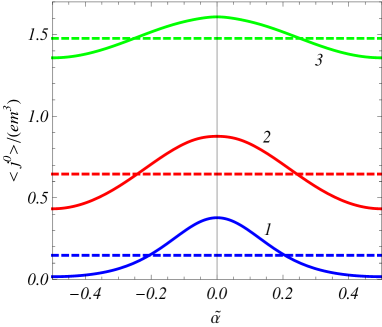
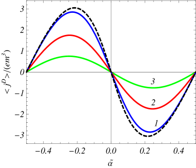
Figure 1: Charge (left panel) and current (right panel) densities as functions of $\tilde{\alpha}$ in $D=3$ model with a single compact dimension for the values of the parameters $\mu/m=0.5$, $mL_{3}=0.5$. The curves are labelled with the value of $T/m$. On the left panel, the dashed lines correspond to the charge density in Minkowski spacetime with trivial topology. The dashed curve on the right panel presents the VEV of the current density.

For the case $|\mu|>$ $\varepsilon_{0}$, in a way similar to that we have used for the FC, assuming that $\mu>0$, the charge density is presented as

$$\left\langle j^{0}\right\rangle = \left\langle j^{0}\right\rangle_{-}+\frac{(4\pi)^{-p/2}eN}{\Gamma(p/2)V_{q}}\sum_{\varepsilon_{\mathbf{n}_{q}}\leqslant\varepsilon_{\mathbf{n}_{q}^{(0)}}}\int_{\varepsilon_{\mathbf{n}_{q}}}^{\infty}dx\,\frac{x(x^{2}-\varepsilon_{\mathbf{n}_{q}}^{2})^{p/2-1}}{e^{\beta(x-\mu)}+1}$$ (3.17)

$$-\frac{Ne\beta}{(2\pi)^{(p+1)/2}V_{q}}\sum_{n=1}^{\infty}(-1)^{n}ne^{n\beta\mu}\sum_{\varepsilon_{\mathbf{n}_{q}}>\varepsilon_{\mathbf{n}_{q}^{(0)}}}\varepsilon_{\mathbf{n}_{q}}^{p+1}f_{(p+1)/2}(n\beta\varepsilon_{\mathbf{n}_{q}}),$$

where the part coming from the antiparticles, $\left\langle j^{0}\right\rangle_{-}$, is given by the same expression (3.6) as before. In the limit $T\rightarrow 0$ we get

$$\left\langle j^{0}\right\rangle=\frac{(4\pi)^{-p/2}eN}{p\Gamma(p/2)V_{q}}\sum_{\varepsilon_{\mathbf{n}_{q}}\leqslant\varepsilon_{\mathbf{n}_{q}^{(0)}}}(\mu^{2}-\varepsilon_{\mathbf{n}_{q}}^{2})^{p/2}.$$ (3.18)

Note that the number of states per unit volume with the energies smaller than $\mu$ is equal to

$$\mathcal{N}_{\leqslant\mu}=\frac{N}{2(2\pi)^{p}V_{q}}\sum_{\varepsilon_{\mathbf{n}_{q}}\leqslant\varepsilon_{\mathbf{n}_{q}^{(0)}}}\int_{|\mathbf{k}_{p}|\leqslant\sqrt{\mu^{2}-\varepsilon_{\mathbf{n}_{q}}^{2}}}d\mathbf{k}_{p}.$$ (3.19)

Now the charge density at zero temperatures can be written as $\left\langle j^{0}\right\rangle_{T=0}=e\mathcal{N}_{\leqslant\mu}$. At high temperatures, the leading term in the expansion of the charge density, as before, is given by Eq. (3.15).

In the discussion above we have considered the charge density as a function of the temperature, chemical potential, and the lengths of compact dimensions. From the physical point of view it is also of interest to consider the behavior of the system for a fixed value of the charge $Q=V_{q}\left\langle j^{0}\right\rangle$. In this case the expressions derived in this section give the chemical potential as a function of the charge, temperature and of the volume of the compact subspace. For example, we can use the formula which follows from Eqs. (3.4) and (3.5):

$$Q=\frac{(4\pi)^{-p/2}eN}{\Gamma(p/2)}\sum_{\mathbf{n}_{q}\in\mathbf{Z}^{q}}\int_{\varepsilon_{\mathbf{n}_{q}}}^{\infty}dx\,x\,\sum_{j=\pm}j\frac{(x^{2}-\varepsilon_{\mathbf{n}_{q}}^{2})^{p/2-1}}{e^{\beta(x-j\mu)}+1}.$$ (3.20)

From here it directly follows that the sign of $\mu$ coincides with the sign of $Q$, consequently $\mu Q>0$, and that the chemical potential is an odd function of $Q$. For fixed temperature and lengths of compact dimensions, the function $|\mu|$ monotonically increases with increasing $|Q|$. At high temperatures, by taking into account that $Q\approx V_{q}\left\langle j^{0}\right\rangle_{\mathrm{M}}$, up to exponentially small terms, and using Eq. (3.15), in the leading order we get

$$\mu\approx\frac{\left(1-2^{2-D}\right)^{-1}}{\Gamma((D+1)/2)\zeta_{\mathrm{R}}(D-1)}\frac{\pi^{(D+1)/2}Q}{eNV_{q}T^{D-1}}.$$ (3.21)

With decreasing the temperature, the chemical potential increases and its value at the zero temperature is determined from Eq. (3.18).

On the left panel of figure 2, for the $D=3$ model with a single compact dimension of the length $L_{3}$ ($p=2$, $q=1$), we plotted the chemical potential as a function of the temperature for a fixed value of the charge corresponding to $Q/(em^{2})=2$ and for $mL_{3}=0.25$. The numbers near the curves correspond to the values of the phase $\tilde{\alpha}_{3}=\tilde{\alpha}$. The dashed curve presents the chemical potential in $D=3$ Minkowski spacetime with trivial topology $R^{3}$ and with the same charge density corresponding to $\left\langle j^{0}\right\rangle_{\mathrm{M}}L_{3}/(em^{2})=2$. The right panel displays the chemical potential as a function of $\tilde{\alpha}$ for the same value of the charge $Q/(em^{2})=2$ and for $T/m=1$. The numbers near the curves correspond to the values of $mL_{3}$.

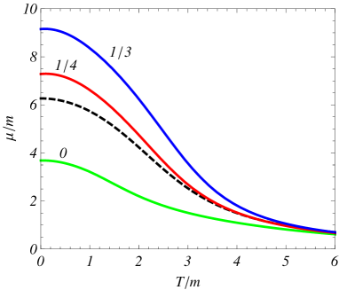
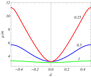
Figure 2: The chemical potential as a function of the temperature (left panel) and of the phase $\tilde{\alpha}$ (right panel) in the $D=3$ model with a single compact dimension. The graphs are plotted for a fixed value of the charge corresponding to $Q/(em^{2})=2$. For the left panel $mL_{3}=0.25$ and the numbers near the curves are the corresponding values of the phase $\tilde{\alpha}$. The dashed curve presents the chemical potential in the Minkowski spacetime with trivial topology. For the right panel $T/m=1$, and the curves are labelled with the value of $mL_{3}$.

4 Current density

Now let us consider the spatial components of the expectation value $\left\langle j^{\nu}\right\rangle$. Substituting the mode functions (2.16) into Eq. (3.2) we get

$$\left\langle j^{\nu}\right\rangle=\left\langle j^{\nu}\right\rangle_{0}+\sum_{j=+,-}\left\langle j^{\nu}\right\rangle_{j},$$ (4.1)

where the contributions from the particles ($j=+$) and antiparticles ($j=-$) are given by the expression below,

$$\left\langle j^{\nu}\right\rangle_{\pm}=\frac{eN}{2(2\pi)^{p}V_{q}}\int d\mathbf{k}_{p}\sum_{\mathbf{n}_{q}\in\mathbf{Z}^{q}}\frac{\tilde{k}_{\nu}/\varepsilon(\mathbf{k})}{e^{\beta(\varepsilon(\mathbf{k})\mp\mu)}+1},$$ (4.2)

for $\nu=1,\ldots,D$. In the case of $\nu=1,\ldots,p$, the integrand is an odd function of $k_{\nu}$ and the integral is zero. Hence, the current density along uncompactified dimensions vanishes: $\left\langle j^{\nu}\right\rangle=0$, $\nu=1,\ldots,p$.

Under the condition $|\mu|<$ $\varepsilon_{0}$, by using Eq. (2.26), and after the integration over $\mathbf{k}_{p}$, we find

$$\left\langle j^{\nu}\right\rangle_{\pm}=-\frac{eN}{(2\pi)^{(p+1)/2}V_{q}}\sum_{n=1}^{\infty}(-1)^{n}e^{\pm n\beta\mu}\sum_{\mathbf{n}_{q}\in\mathbf{Z}^{q}}\tilde{k}_{\nu}\varepsilon_{\mathbf{n}_{q}}^{p-1}f_{(p-1)/2}(n\beta\varepsilon_{\mathbf{n}_{q}}),$$ (4.3)

for the current densities coming from particles/antiparticles, and

$$\left\langle j^{\nu}\right\rangle=\left\langle j^{\nu}\right\rangle_{0}-\frac{2eN}{(2\pi)^{(p+1)/2}V_{q}}\sum_{n=1}^{\infty}(-1)^{n}\cosh(n\beta\mu)\sum_{\mathbf{n}_{q}\in\mathbf{Z}^{q}}\tilde{k}_{\nu}\varepsilon_{\mathbf{n}_{q}}^{p-1}f_{(p-1)/2}(n\beta\varepsilon_{\mathbf{n}_{q}}),$$ (4.4)

for the total current density. From Eq. (4.4) it follows that the current density along the $\nu$th compact dimension is an even function of the phases $\tilde{\alpha}_{l}$, $l\neq\nu$, and an odd function of the phase $\tilde{\alpha}_{\nu}$. In particular, $\left\langle j^{\nu}\right\rangle=0$ for $\tilde{\alpha}_{\nu}=0$. The latter is the case for twisted and untwisted fields in the absence of magnetic fluxes. At low temperatures regime, the dominant contribution to the finite temperature part comes from the mode with the lowest energy and, to the leading order, one has

$$\left\langle j^{\nu}\right\rangle=\left\langle j^{\nu}\right\rangle_{0}+\frac{eN\tilde{\alpha}_{\nu}\varepsilon_{0}^{p/2-1}e^{-\beta(\varepsilon_{0}-|\mu|)}}{2(2\pi)^{p/2-1}V_{q}L_{\nu}\beta^{p/2}}.$$ (4.5)

In this limit, the finite temperature part is exponentially suppressed.

Another form for the current density is obtained on the base of the zeta function approach. With this aim, we write Eq. (4.2) as

$$\left\langle j^{\nu}\right\rangle=-\frac{eN}{(2\pi)^{p}V_{q}}\int d\mathbf{k}_{p}\sum_{\mathbf{n}_{q}\in\mathbf{Z}^{q}}\frac{\tilde{k}_{\nu}}{\varepsilon(\mathbf{k})}\sideset{}{{}^{\prime}}{\sum}_{n=0}^{\infty}(-1)^{n}\cosh(n\beta\mu)e^{-n\beta\varepsilon(\mathbf{k})}.$$ (4.6)

By using Eqs. (2.34) and (2.35), this expression is presented in the form

$$\left\langle j^{\nu}\right\rangle=-\frac{eN}{L_{\nu}}\sum_{n_{\nu}=-\infty}^{+\infty}\tilde{k}_{\nu}\zeta_{\nu}(1),$$ (4.7)

where the partial zeta function is defined as

$$\zeta_{\nu}(s)=\frac{L_{\nu}}{\beta V_{q}}\int\frac{d\mathbf{k}_{p}}{(2\pi)^{p}}\sum_{\mathbf{n}_{q}^{\nu}\in\mathbf{Z}^{q}}(\mathbf{k}_{p}^{2}+\sum_{l=p+1}^{D+1}\tilde{k}_{l}^{2}+m^{2})^{-s},$$ (4.8)

with $\mathbf{n}_{q}^{\nu}=(n_{p+1},\ldots,n_{\nu-1},n_{\nu+1},\ldots,n_{D+1})$. Here, $\tilde{k}_{D+1}=2\pi(n_{D+1}+\tilde{\alpha}_{D+1})/L_{D+1}$ with $L_{D+1}$ and $\tilde{\alpha}_{D+1}$ being given by Eq. (2.38).

After the integration over $\mathbf{k}_{p}$ and the application of the generalized Chowla-Selberg formula [21], the following representation is obtained:

$$\zeta_{\nu}(s) = \frac{m_{\nu}^{D-2s}}{(4\pi)^{D/2}}\frac{\Gamma(s-D/2)}{\Gamma(s)}+\frac{2^{1-s}m_{\nu}^{D-2s}}{(2\pi)^{D/2}\Gamma(s)}$$ (4.9)

$$\times\sideset{}{{}^{\prime}}{\sum}_{\mathbf{n}_{q}^{\nu}\in\mathbf{Z}^{q}}\cos(2\pi\mathbf{n}_{q}^{\nu}\cdot\boldsymbol{\alpha}_{q}^{\nu})f_{D/2-s}(m_{\nu}g(\mathbf{L}_{q}^{\nu},\mathbf{n}_{q}^{\nu})),$$

where $\mathbf{L}_{q}=(L_{p+1},\ldots,L_{\nu-1},L_{\nu+1},\ldots L_{D},\beta)$, $\boldsymbol{\alpha}_{q}^{\nu}=(\tilde{\alpha}_{p+1},\ldots,\tilde{\alpha}_{\nu-1},\tilde{\alpha}_{\nu+1},\ldots,\tilde{\alpha}_{D+1})$ and

$$m_{\nu}=\sqrt{\tilde{k}_{\nu}^{2}+m^{2}}.$$ (4.10)

The contribution of the second term in the right-hand side of Eq. (4.9) to the current density is finite at the physical point $s=1$. The analytical continuation of the first term is obtained by applying the summation formula (2.50) to the series over $n_{\nu}$. In this way, we get

$$\frac{\Gamma(s-D/2)}{(4\pi)^{D/2}\Gamma(s)}\sum_{n_{\nu}=-\infty}^{+\infty}\frac{\tilde{k}_{\nu}}{m_{\nu}^{2s-D}}$$

$$\quad=2L_{\nu}\frac{(2m)^{(D+1-2s)/2+1}}{(4\pi)^{(D+1)/2}\Gamma(s)}\sum_{n=1}^{\infty}\sin(2\pi n\tilde{\alpha}_{\nu})\frac{K_{(D+1-2s)/2+1}(nL_{\nu}m)}{(nL_{\nu})^{(D+1-2s)/2}}.$$ (4.11)

Combining Eqs. (4.9) and (4.11), for the current density along the $\nu$th compact dimension we find

$$\left\langle j^{\nu}\right\rangle = \left\langle j^{\nu}\right\rangle_{D-1,1}-\frac{2eNL_{\nu}^{-1}}{(2\pi)^{D/2}}\sideset{}{{}^{\prime}}{\sum}_{n=0}^{\infty}(-1)^{n}\cosh(n\beta\mu)\sum_{n_{\nu}=-\infty}^{+\infty}\tilde{k}_{\nu}m_{\nu}^{D-2}$$ (4.12)

$$\times\sum_{\mathbf{n}_{q-1}^{\nu}\in\mathbf{Z}^{q-1}}\cos(2\pi\mathbf{n}_{q-1}^{\nu}\cdot\boldsymbol{\alpha}_{q-1}^{\nu})f_{D/2-1}(m_{\nu}(\sum_{i=p+1,\neq\nu}^{D}L_{i}^{2}n_{i}^{2}+n^{2}\beta^{2})^{1/2}).$$

where the term $n=0$, $\mathbf{n}_{q-1}^{\nu}=0$ is excluded, $\mathbf{n}_{q-1}^{\nu}=(n_{p+1},\ldots,n_{\nu-1},n_{\nu+1},\ldots,n_{D})$, $\boldsymbol{\alpha}_{q-1}^{\nu}=(\tilde{\alpha}_{p+1},\ldots,\tilde{\alpha}_{\nu-1},\tilde{\alpha}_{\nu+1},\ldots\tilde{\alpha}_{D})$, and

$$\left\langle j^{\nu}\right\rangle_{D-1,1}=-\frac{2eNm^{D+1}L_{\nu}}{(2\pi)^{(D+1)/2}}\sum_{l=1}^{\infty}l\sin(2\pi l\tilde{\alpha}_{\nu})f_{(D+1)/2}(lL_{\nu}m),$$ (4.13)

is the zero temperature current density for the topology $R^{D-1}\times S^{1}$ with the compact dimension of the length $L_{\nu}$. A more compact form is obtained by making use of the relation

$$\sum_{n_{\nu}=-\infty}^{+\infty}\tilde{k}_{\nu}m_{\nu}^{D-2}f_{D/2-1}(m_{\nu}y)$$

$$\quad=\sqrt{\frac{2}{\pi}}L_{\nu}^{2}m^{D+1}\sum_{n_{\nu}=1}^{\infty}n_{\nu}\sin(2\pi n_{\nu}\tilde{\alpha}_{\nu})f_{(D+1)/2}(m\sqrt{y^{2}+n_{\nu}^{2}L_{\nu}^{2}}).$$ (4.14)

This leads to the final result:

$$\left\langle j^{\nu}\right\rangle = -\frac{4eNm^{D+1}L_{\nu}}{(2\pi)^{(D+1)/2}}\sideset{}{{}^{\prime}}{\sum}_{n=0}^{\infty}(-1)^{n}\cosh(n\beta\mu)\sum_{n_{\nu}=1}^{\infty}n_{\nu}\sin(2\pi n_{\nu}\tilde{\alpha}_{\nu})$$ (4.15)

$$\times\sum_{\mathbf{n}_{q-1}^{\nu}\in\mathbf{Z}^{q-1}}\cos(2\pi\mathbf{n}_{q-1}^{\nu}\cdot\boldsymbol{\alpha}_{q-1}^{\nu})f_{(D+1)/2}(m\sqrt{g^{2}(\mathbf{L}_{q},\mathbf{n}_{q})+n^{2}\beta^{2}}).$$

The $n=0$ term in this formula corresponds to the VEV of the current density:

$$\left\langle j^{\nu}\right\rangle_{0} = -\frac{2eNm^{D+1}L_{\nu}}{(2\pi)^{(D+1)/2}}\sum_{n_{\nu}=1}^{\infty}n_{\nu}\sin(2\pi n_{\nu}\tilde{\alpha}_{\nu})$$ (4.16)

$$\times\sum_{\mathbf{n}_{q-1}^{\nu}\in\mathbf{Z}^{q-1}}\cos(2\pi\mathbf{n}_{q-1}^{\nu}\cdot\boldsymbol{\alpha}_{q-1}^{\nu})f_{(D+1)/2}(mg(\mathbf{L}_{q},\mathbf{n}_{q})).$$

In order to see the asymptotic behavior of the current density at high temperatures, we apply to the series over $n$ in Eq. (4.15) the formula (2.46). This leads to the expression

$$\left\langle j^{\nu}\right\rangle = -\frac{2eNL_{\nu}T}{(2\pi)^{D/2}}\sum_{n_{\nu}=1}^{\infty}n_{\nu}\sin(2\pi n_{\nu}\tilde{\alpha}_{\nu})\sum_{n=-\infty}^{+\infty}\left[(\pi(2n+1)T+i\mu)^{2}+m^{2}\right]^{D/2}$$ (4.17)

$$\times\sum_{\mathbf{n}_{q-1}^{\nu}\in\mathbf{Z}^{q-1}}\cos(2\pi\mathbf{n}_{q-1}^{\nu}\cdot\boldsymbol{\alpha}_{q-1}^{\nu})f_{D/2}(g(\mathbf{L}_{q},\mathbf{n}_{q})\sqrt{(\pi(2n+1)T+i\mu)^{2}+m^{2}}).$$

At high temperatures the dominant contribution comes from the terms $n=-1,0$ in the series over $n$ and from the term with $n_{l}=\delta_{l\nu}$. To the leading order, we get

$$\left\langle j^{\nu}\right\rangle\approx-\frac{2eN\sin(2\pi\tilde{\alpha}_{\nu})T^{(D+1)/2}}{(2L_{\nu})^{(D-1)/2}e^{\pi L_{\nu}T}},$$ (4.18)

and the current density is exponentially suppressed. This is in sharp contrast with the high-temperature behavior of the current density in the case of a scalar field. At high temperatures, the current density for a scalar field linearly grows with the temperature [15]. This difference of the asymptotics for scalar and fermionic current densities is a direct consequence of different periodicity conditions imposed on the fields along imaginary time (periodic and antiperiodic conditions for scalar and fermion fields, respectively).

An alternative representation for the current density is obtained by applying the summation formula (2.50) to the series over $n_{\nu}$ in Eq. (4.6) by taking $g(x)=x$ and the function $f(x)$ from Eq. (2.51). With this choice, the first term in the right-hand side of Eq. (2.50) vanishes, and for the current density one gets

$$\left\langle j^{\nu}\right\rangle = -\frac{4eNL_{\nu}^{2}}{(2\pi)^{p/2+1}V_{q}}\sideset{}{{}^{\prime}}{\sum}_{n=0}^{\infty}(-1)^{n}\cosh(n\beta\mu)\sum_{l=1}^{\infty}l\sin(2\pi l\tilde{\alpha}_{\nu})$$ (4.19)

$$\times\sum_{\mathbf{n}_{q-1}^{\nu}\in\mathbf{Z}^{q-1}}\varepsilon_{\mathbf{n}_{q-1}^{\nu}}^{p+2}f_{p/2+1}(\varepsilon_{\mathbf{n}_{q-1}^{\nu}}\sqrt{l^{2}L_{\nu}^{2}+n^{2}\beta^{2}}).$$

The $n=0$ term in this expression corresponds to the VEV of the current density:

$$\left\langle j^{\nu}\right\rangle_{0}=-\frac{2eNL_{\nu}^{2}}{(2\pi)^{p/2+1}V_{q}}\sum_{l=1}^{\infty}l\sin(2\pi l\tilde{\alpha}_{\nu})\sum_{\mathbf{n}_{q-1}^{\nu}\in\mathbf{Z}^{q-1}}\varepsilon_{\mathbf{n}_{q-1}^{\nu}}^{p+2}f_{p/2+1}(lL_{\nu}\varepsilon_{\mathbf{n}_{q-1}^{\nu}}).$$ (4.20)

In the model with a single compact dimension Eq. (4.19) is reduced to Eq. (4.13).

Let us consider the limit of Eq. (4.19) when the length of the $r$th dimension is much smaller than $L_{\nu}$, $L_{r}\ll L_{\nu}$. The current density is a periodic function of $\tilde{\alpha}_{r}$ with the period equal to unity and, without loss of generality, we can assume that $|\tilde{\alpha}_{r}|<1/2$. If $\tilde{\alpha}_{r}=0$, the dominant contribution comes from the term $n_{r}=0$ and, to the leading order, we have $\left\langle j^{\nu}\right\rangle\approx N\left\langle j^{\nu}\right\rangle_{(p,q-1)}/(N_{D-1}L_{r})$, where $\left\langle j^{\nu}\right\rangle_{(p,q-1)}$ is the current density in $(D-1)$-dimensional space of topology $R^{p}\times(S^{1})^{q-1}$ with the lengths of the compact dimensions $L_{p+1}$,…,$L_{r-1}$,$L_{r+1}$,…,$L_{D}$. The corrections to this leading term are of the order $e^{-2\pi L_{\nu}/L_{r}}$. For $\tilde{\alpha}_{r}\neq 0$, once again, the dominant contribution comes from the term with $n_{r}=0$, and the argument of the function $f_{p/2+1}(x)$ in Eq. (4.19) is large. By using the corresponding asymptotic for the Macdonald function, we see that the current density is suppressed by the factor $e^{-2\pi|\tilde{\alpha}_{r}|L_{\nu}/L_{r}}$.

The right panel of figure 1, displays the current density in the $D=3$ model with a single compact dimension, as a function of $\tilde{\alpha}_{3}\equiv\tilde{\alpha}$ for $\mu/m=0.5$ and $mL_{3}=0.5$. The numbers near the curves are the correspond values of $T/m$. The dashed curve presents the current density at zero temperature.

Now we turn to the case $|\mu|>$ $\varepsilon_{0}$. After the integration in Eq. (4.2), the general formula (4.1) is given in the form

$$\left\langle j^{\nu}\right\rangle=\left\langle j^{\nu}\right\rangle_{0}+\frac{(4\pi)^{-p/2}eN}{\Gamma(p/2)V_{q}}\sum_{\mathbf{n}_{q}\in\mathbf{Z}^{q}}\tilde{k}_{\nu}\int_{\varepsilon_{\mathbf{n}_{q}}}^{\infty}dx\,\sum_{j=+,-}\frac{(x^{2}-\varepsilon_{\mathbf{n}_{q}}^{2})^{p/2-1}}{e^{\beta(x-j\mu)}+1}.$$ (4.21)

For definiteness, assuming that $\mu>0$, the transformations for the part with $j=-$ and for the part $j=+$ in the range $\varepsilon_{\mathbf{n}_{q}}>\mu$ are the same as those described above. For the current density along the $\nu$th compact dimension one finds:

$$\left\langle j^{\nu}\right\rangle = \left\langle j^{\nu}\right\rangle_{0}+\left\langle j^{\nu}\right\rangle_{-}+\frac{(4\pi)^{-p/2}eN}{\Gamma(p/2)V_{q}}\sum_{\varepsilon_{\mathbf{n}_{q}}\leqslant\varepsilon_{\mathbf{n}_{q}^{(0)}}}\tilde{k}_{\nu}\int_{\varepsilon_{\mathbf{n}_{q}}}^{\infty}dx\,\frac{(x^{2}-\varepsilon_{\mathbf{n}_{q}}^{2})^{p/2-1}}{e^{\beta(x-\mu)}+1}$$ (4.22)

$$-\frac{eN}{(2\pi)^{(p+1)/2}V_{q}}\sum_{n=1}^{\infty}(-1)^{n}e^{n\beta\mu}\sum_{\varepsilon_{\mathbf{n}_{q}}>\varepsilon_{\mathbf{n}_{q}^{(0)}}}\tilde{k}_{\nu}\varepsilon_{\mathbf{n}_{q}}^{p-1}f_{(p-1)/2}(n\beta\varepsilon_{\mathbf{n}_{q}}).$$

In the limit $T\rightarrow 0$ we get

$$\left\langle j^{\nu}\right\rangle_{T=0}=\left\langle j^{\nu}\right\rangle_{0}+\frac{(4\pi)^{-p/2}eN}{V_{q}\Gamma(p/2)}\sum_{\varepsilon_{\mathbf{n}_{q}}\leqslant\varepsilon_{\mathbf{n}_{q}^{(0)}}}\tilde{k}_{\nu}\int_{\varepsilon_{\mathbf{n}_{q}}}^{\mu}dx\,(x^{2}-\varepsilon_{\mathbf{n}_{q}}^{2})^{p/2-1}.$$ (4.23)

The second term on the right is the current density induced by the particles filling the states with the energies $\varepsilon_{\mathbf{n}_{q}}\leq\mu$. At zero temperature the states with the energies $\varepsilon_{\mathbf{n}_{q}}>\mu$ are empty. At high temperatures, similar to the case $|\mu|<$ $\varepsilon_{0}$, the current density is exponentially suppressed (see Eq. (4.18)).

For a fixed value of the charge, Eq. (3.20) determines the chemical potential as a function of temperature. Examples of this function are plotted in figure 2. Substituting the chemical potential into Eq. (4.21) or Eq. (4.22), we find the current density as a function of the temperature for a fixed value of the charge. On the left panel of figure 3 we have plotted this function in the $D=3$ model with a single compact dimension of the length $L_{3}$, for the fixed value of the charge corresponding to $Q/(em^{2})=2$. The graphs are plotted for $mL_{3}=0.25$ and the numbers near the curves correspond to the values of $\tilde{\alpha}_{3}=\tilde{\alpha}$. The right panel presents the current density versus the phase $\tilde{\alpha}$ for different values of $Q/(em^{2})$ (numbers near the curves) and for $T/m=0.5$, $mL_{3}=0.5$.

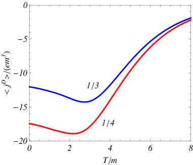
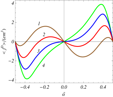
Figure 3: The current density for a fixed value of the charge as a function of the temperature (left panel) and of the phase $\tilde{\alpha}$ (right panel) in $D=3$ model with a single compact dimension. On the left panel the graphs are plotted for $Q/(em^{2})=2$, $mL_{3}=0.25$ and the curves are labelled with the value of $\tilde{\alpha}$. For the right panel $T/m=0.5$, $mL_{3}=0.5$, and the numbers near the curves correspond to the values of $Q/(em^{2})$.

5 Expectation values in time-reversal symmetric odd dimensional models

In the discussion above we have considered a fermionic field realizing the irreducible representation of the Clifford algebra. With this representation, in odd dimensional spacetimes ($D$ is an even number) the mass term in the Lagrangian breaks $C$-invariance in $D=4n$, $P$-invariance in $D=4n,4n+2$, and $T$-invariance in $D=4n+2$ (for a general discussion see Ref. [23]). In order to restore these symmetries, we note that in odd dimensions the $\gamma^{D}$ matrix can be represented by other gamma matrices in the following way,

$$\gamma^{D}=\gamma_{\pm}^{D}=\left\{\begin{array}[]{cc}\pm\gamma,&D=4n,\\ \pm i\gamma,&D=4n+2,\end{array}\right.$$ (5.1)

where $\gamma=\gamma^{0}\gamma^{1}\cdots\gamma^{D-1}$. Hence, the Clifford algebra in odd dimensions has two inequivalent representations corresponding to the upper and lower signs in Eq. (5.1). Now, two $N$-component Dirac fields, $\psi_{+}$ and $\psi_{-}$, can be introduced with the equations

$$(i\gamma_{\pm}^{\mu}D_{\mu}-m)\psi_{\pm}=0,$$ (5.2)

where $\gamma_{\pm}^{\mu}=(\gamma^{0},\gamma^{1},\cdots\gamma^{D-1},\gamma_{\pm}^{D})$. Defining the charge conjugation as $\psi_{+}^{C}=C\bar{\psi}_{-}^{T}$ (for $C$, $P$ and $T$ transformations, see, for instance, Ref. [23]), we see that the total Lagrangian $\mathcal{L}=\sum_{j=+,-}\bar{\psi}_{j}(i\gamma_{j}^{\mu}D_{\mu}-m)\psi_{j}$ is invariant under the charge conjugation. In a similar way, by suitable transformations of the fields it can be seen that the combined Lagrangian is invariant under $P$ and $T$ transformations, as well (in the absence of magnetic fields). Note that by defining new fields $\psi_{+}^{\prime}=\psi_{+}$, $\psi_{-}^{\prime}=\gamma\psi_{-}$, the Lagrangian is transformed to the form

$$\mathcal{L}=\sum_{j=+,-}\bar{\psi}_{j}^{\prime}(i\gamma^{\mu}D_{\mu}-jm)\psi_{j}^{\prime}.$$ (5.3)

Thus, the field $\psi_{-}^{\prime}$ satisfies the same equation as $\psi_{+}^{\prime}$ with the opposite sign for the mass term. The $N$-component Dirac spinors $\psi_{+}^{\prime}$ and $\psi_{-}^{\prime}$ can be combined in a $2N$-component spinor: $\Psi=(\psi_{+}^{\prime},\psi_{-}^{\prime})^{T}$. Introducing $2N\times 2N$ Dirac matrices $\tilde{\gamma}^{\mu}=I_{2}\otimes\gamma^{\mu}$ and $\eta=\sigma_{\mathrm{P}3}\otimes I_{N}$, where $I_{N}$ is the $N\times N$ unit matrix and $\sigma_{\mathrm{P}3}=\mathrm{diag}(1,-1)$ the Pauli matrix, the Lagrangian is written in the form $\mathcal{L}=\bar{\Psi}(i\tilde{\gamma}^{\mu}D_{\mu}-m\eta)\Psi$. An alternative representation is obtained by using the $2N\times 2N$ reducible representation of gamma matrices $\gamma_{(2N)}^{\mu}=\sigma_{3}\otimes\gamma^{\mu}$ with the Lagrangian

$$\mathcal{L}=\bar{\Psi}(i\gamma_{(2N)}^{\mu}D_{\mu}-m)\Psi.$$ (5.4)

The FC, the charge and current densities for the model described by the Lagrangian (5.3) can be obtained from the formulas given above. In deriving the expectation values of these quantities we have assumed that the parameter $m$ is nonnegative. However, the results are easily generalized for a negative $m$ as well. It can be seen that $\left\langle\bar{\psi}\psi\right\rangle/m$ and $\left\langle j^{\mu}\right\rangle$ are even functions of $m$. Consequently, the current densities corresponding to the fields $\psi_{+}^{\prime}$ and $\psi_{-}^{\prime}$ are given by expressions presented in Sections 3 and 4 whereas the FC for the fields $\psi_{+}^{\prime}$ and $\psi_{-}^{\prime}$ differ by the sign. Hence, assuming that in Eq. (5.3) $m\geqslant 0$, for the total expectation values one finds

$$\left\langle\bar{\Psi}\Psi\right\rangle = \left\langle\bar{\psi}\psi\right\rangle_{\uparrow}-\left\langle\bar{\psi}\psi\right\rangle_{\downarrow},$$

$$\left\langle j^{\nu}\right\rangle = \left\langle j^{\nu}\right\rangle_{\uparrow}+\left\langle j^{\nu}\right\rangle_{\downarrow},$$ (5.5)

where the parts with the indices $\uparrow$ and $\downarrow$ are the contributions coming from the upper ($\psi_{+}^{\prime}$) and lower ($\psi_{-}^{\prime}$) components of the $2N$-component spinor $\Psi$. The separate terms in (5.5), $\left\langle\bar{\psi}\psi\right\rangle_{\uparrow,\downarrow}$ and $\left\langle j^{\nu}\right\rangle_{\uparrow,\downarrow}$ are given by the expressions presented in Sections 3 and 4. If the phases in the quasiperiodicity conditions for the upper and lower components of the $2N$-spinor $\Psi$ are the same, then the resulting FC vanishes, whereas the expressions for the charge and current densities are obtained from the expressions given above with an additional coefficient 2. However, the phases in the quasiperiodicity conditions for the upper and lower components, in general, can be different. As we will see below, this is the case for the Dirac model in a class of carbon nanotubes.

6 Applications to carbon nanotubes

In this section we apply the general results given above for the investigation of the FC and current density in carbon nanotubes (for a review see Ref. [24]). A single-wall cylindrical nanotube is obtained from a graphene sheet by rolling it into a cylindrical shape. In graphene, the low-energy excitations of the electronic subsystem, for a given value of spin $s=\pm 1$, are described by an effective Dirac theory of 4-component spinors $\Psi_{s}=(\psi_{+,As},\psi_{+,Bs},\psi_{-,As},\psi_{-,Bs})$, where the components $\psi_{\pm,Js}$, with $J=A$ and $J=B$, give the amplitude of the wave function on the $A$ and $B$ triangular sublattices of the graphene hexagonal lattice and the indices $+$ and $-$ correspond to inequivalent points $(\mathbf{K}_{+},\mathbf{K}_{-})$ at the corners of the two-dimensional Brillouin zone (see Ref. [3]). The quasiparticles are confined to a graphene sheet and, hence, for the spatial dimension of the corresponding Dirac-like theory one has $D=2$. The corresponding Lagrangian has the form (we restore the standard units)

$$\mathcal{L}=\sum_{s=\pm 1}\bar{\Psi}_{s}(i\hbar\gamma^{0}\partial_{t}+i\hbar v_{F}\gamma^{l}D_{l}-\Delta)\Psi_{s},$$ (6.1)

where $D_{l}=(\mathbf{\nabla}-ie\mathbf{A}/\hbar c)_{l}$, $l=1,2$, with $e=-|e|$ for electrons, and $v_{F}\approx 7.9\times 10^{7}$ cm/s is the Fermi velocity which plays the role of the speed of light. (For other planar condensed-matter systems with the low-energy sector described by Eq. (6.1) see, for instance, Ref. [25].) For the Fermi velocity one has $v_{F}=\sqrt{3}a\gamma_{0}/(2\hbar)$, where $a$ is the lattice constant and $\gamma_{0}\approx 2.9$ eV is the transfer integral between first-neighbor $\pi$ orbitals. We have included in the Lagrangian the energy gap $\Delta$. It is expressed in terms of the corresponding Dirac mass $m_{D}$ as $\Delta=m_{D}v_{F}^{2}$. The gap in the energy spectrum is essential in many physical applications and can be generated by a number of mechanisms (see, for example, Ref. [3] and references therein). Some mechanisms give rise to mass terms with the matrix structure different from that we consider here. In dependence of the physical mechanism for the generation, the energy gap may vary in the range $1\,\mathrm{meV}\lesssim\Delta\lesssim 1\,\mathrm{eV}$. In the discussion of the graphene properties within the framework of the model described by Lagrangian (6.1), the Dirac matrices are usually taken in the form $\gamma^{\mu}=\sigma_{\mathrm{P}3}\otimes(\sigma_{\mathrm{P}3},i\sigma_{\mathrm{P}2},-i\sigma_{\mathrm{P}1})$. Now comparing with Eq. (5.4), we see that Eq. (6.1) is a special case with $D=2$, $N=2$.

In the case of the cylindrical nanotube, the spatial topology for the effective Dirac theory is $R^{1}\times S^{1}$ with the compactified dimension of the length $L$. The carbon nanotube is characterized by its chiral vector $\mathbf{C}_{h}=n_{c}\mathbf{a}_{1}+m_{c}\mathbf{a}_{2}$, where $\mathbf{a}_{1}$ and $\mathbf{a}_{2}$ are the basis vectors of the hexagonal lattice of graphene and $n_{c}$, $m_{c}$ are integers. The length of the compact dimension is given by $L=|\mathbf{C}_{h}|=aN_{c}$, with $N_{c}=\sqrt{n_{c}^{2}+m_{c}^{2}+n_{c}m_{c}}$ and $a=|\mathbf{a}_{1}|=|\mathbf{a}_{2}|=2.46\mathring{A}$ being the lattice constant. The special cases $\mathbf{C}_{h}=(n_{c},0)$ and $\mathbf{C}_{h}=(n_{c},n_{c})$ correspond to zigzag and armchair nanotubes respectively. All other cases correspond to chiral nanotubes. In the case $n_{c}-m_{c}=3l_{c}$, $l_{c}\in Z$, the nanotube will be metallic and in the case $n_{c}-m_{c}\neq 3l_{c}$ the nanotube will be a semiconductor with an energy gap inversely proportional to the diameter. In particular, the armchair nanotube is metallic, and the $(n_{c},0)$ zigzag nanotube is metallic if and only if $n_{c}$ is an integer multiple of 3.

Periodicity conditions along the compact dimension for the bi-spinor $\Psi_{s}$ in (6.1) are obtained from the periodicity of the electron wave function (see Refs. [24, 26]). For metallic nanotubes one has periodic boundary conditions ($\alpha_{l}=0$ in Eq. (2.3)) and for semiconducting nanotubes, depending on the chiral vector, we have two classes of inequivalent boundary conditions corresponding to $\alpha_{l}=\pm 1/3$ ($n_{c}-m_{c}=3l_{c}\pm 1$). The phases have opposite signs for the upper and lower components of the 4-spinor $\Psi_{s}$ in (6.1), corresponding to the points $\mathbf{K}_{+}$ and $\mathbf{K}_{-}$.

For a given value of the spin $s$, the expressions of the FC and of the expectation values of the current densities for separate contributions from the points $\mathbf{K}_{+}$ and $\mathbf{K}_{-}$ are obtained from the expressions given in previous sections by the replacements

$$m\rightarrow a^{-1}\Delta/\gamma_{F},\;\beta\rightarrow a\gamma_{F}\beta,\;\mu\rightarrow a^{-1}\mu/\gamma_{F},$$ (6.2)

where $\gamma_{F}=\hbar v_{F}/a=\sqrt{3}\gamma_{0}/2\approx 2.51$ eV determines the characteristic energy scale of the model. In addition, in expressions for the current density along compact dimensions a factor $v_{F}$ should be added, because now the operator of the spatial components of the current density is defined as $j^{\nu}=ev_{F}\bar{\psi}(x)\gamma^{\nu}\psi(x)$. For a given spin $s$, the separate contributions are combined in a way given by Eq. (5.5), where $\uparrow$ and $\downarrow$ correspond to the points $\mathbf{K}_{+}$ and $\mathbf{K}_{-}$, respectively. In the model under consideration, the spin $s=+1$ and $s=-1$ give the same contributions to the total expectation values. For cylindrical carbon nanotubes, the spatial topology for the effective theory corresponds to $R^{1}\times S^{1}$ and, hence, in the formulas above $p=1$, $q=1$.

The compactification of the direction along the cylinder axis gives another class of graphene made structures called toroidal carbon nanotubes [27] with the background topology $(S^{1})^{2}$ ($p=0,q=2$). The nanotorus is classified by its chiral vector $\mathbf{C}_{h}$ and translational vector $\mathbf{T}=p_{c}\mathbf{a}_{1}+q_{c}\mathbf{a}_{2}$ with the coordinates along these directions $z^{1}$ and $z^{2}$ and with the lengths $L_{1}$ and $L_{2}$. Usually one has $L_{1}\ll L_{2}$. From the asymptotic analysis given above (see the paragraph after Eq. (4.20)), it follows that for $\tilde{\alpha}_{1}=0$ the current density along $z^{2}$, in the leading order, coincides with the corresponding quantity in the model with $D=1$ and with the length of the compact dimension $L_{2}$. The corresponding corrections are of the order $e^{-2\pi L_{2}/L_{1}}$. In the absence of the magnetic flux, this case corresponds to nanotubes for which $\alpha_{1}=0$ and, hence, $n_{c}-m_{c}=3l_{c}$, $l_{c}\in Z$, (type I and II toroidal carbon nanotubes). For $\tilde{\alpha}_{1}\neq 0$, the current density along $z^{2}$-direction is suppressed by the factor $e^{-2\pi|\tilde{\alpha}_{1}|L_{2}/L_{1}}$. In the absence of the magnetic flux, this case corresponds to $n_{c}-m_{c}\neq 3l_{c}$, $l_{c}\in Z$, with $|\alpha_{1}|=1/3$ (type III toroidal carbon nanotubes).

In discussing the FC and current density in cylindrical and toroidal nanotubes we work within the zone-folding approximation in which the effect of confinement is to induce the selection on allowed values of the momentum projection along the compact dimension. This approximation ignores the curvature effects which may cause the mixing of $\sigma$ and $\pi$ orbitals of the carbon atoms. These effects are small for nanotubes with a sufficiently large diameter.

6.1 One dimensional rings

Here, we start with the simplest case $D=1$ having a compact dimension of the length $L=aN_{c}$ and with the phase in the periodicity condition $\alpha_{1}=\alpha$. As we have noted, this case can be considered as a model of a toroidal nanotube in the limit when the length of one of the compact dimensions is small compared to the other (for the investigation of persistent currents in toroidal carbon nanotubes within the framework of the tight-binding approximation, see Refs. [28]). For simplicity we consider the case of zero chemical potential when the charge density vanishes. The zero value for the chemical potential is predicted by simple tight-binding calculations for the hexagonal lattice of a single graphene sheet (see, for example, [24]). By using the formulas given in previous sections, the generalization for the case of a nonzero chemical potential is straightforward (for mechanisms of generation of a nonzero chemical potential see Ref. [25]).

By summing the contributions coming from two sublattices with opposite signs of $\alpha$ and adding an additional factor 2 which takes into account the contributions from two spins $s=\pm 1$, for the FC we find

$$\left\langle\bar{\psi}\psi\right\rangle=-\frac{8x_{c}}{\pi L}\sum_{l=1}^{\infty}\sin(2\pi l\alpha)\sin(2\pi l\phi/\phi_{0})K_{0}(lx_{c})+\frac{4x_{c}}{L}\sum_{l=-\infty}^{+\infty}\sum_{j=\pm 1}\frac{j/b_{l}^{(j)}}{e^{b_{l}^{(j)}y_{c}}+1},$$ (6.3)

with the notations

$$x_{c}=N_{c}\Delta/\gamma_{F},\;y_{c}=\gamma_{F}/(N_{c}T),$$ (6.4)

and

$$b_{l}^{(j)}=\sqrt{\kappa_{l}^{(j)2}+x_{c}^{2}},\;\kappa_{l}^{(j)}=2\pi(l+j\alpha-\phi/\phi_{0}).$$ (6.5)

The first term in the right-hand side of Eq. (6.3) gives the FC at zero temperature. As it is seen, the quantity $\gamma_{F}/N_{c}$ determines the characteristic energy scale of the model. For toroidal nanotubes one has $N_{c}\sim 10^{3}$ and this energy scale is of the order of the meV. The corresponding characteristic temperature is $T_{c}=\gamma_{F}/(N_{c}k_{\mathrm{B}})\approx 30\,\mathrm{K}$.

An alternative expression is obtained by making use of Eq. (2.41):

$$\left\langle\bar{\psi}\psi\right\rangle=-\frac{16x_{c}}{\pi L}\sideset{}{{}^{\prime}}{\sum}_{n=0}^{\infty}(-1)^{n}\sum_{l=1}^{\infty}\sin(2\pi l\alpha)\sin(2\pi l\phi/\phi_{0})K_{0}(x_{c}\sqrt{l^{2}+n^{2}y_{c}^{2}}),$$ (6.6)

where the zero-temperature part is given by the term $n=0$. From the asymptotic analysis in Section 2 we see that at high temperatures, $T\gg\gamma_{F}/N_{c}$, the FC is exponentially suppressed:

$$\left\langle\bar{\psi}\psi\right\rangle\approx-\frac{16x_{c}\sin(2\pi l\alpha)}{\pi L}\sin(2\pi l\phi/\phi_{0})e^{-\pi/y_{c}}.$$ (6.7)

An exponential suppression takes place also for large values of the energy gap: $x_{c}\gg 1$. In figure 4 we have plotted the FC, given by Eq. (6.3), as a function of the magnetic flux for $\alpha=1/3$ and $x_{c}=0.5$. The numbers near the curves correspond to the value of $TN_{c}/\gamma_{F}$.

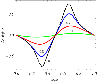
Figure 4: FC as a function of the magnetic flux for $\alpha=1/3$ and $x_{c}=0.5$. The numbers near the curves correspond to the value of $TN_{c}/\gamma_{F}$.

Now we turn to the current density. By summing the contributions coming from two valleys with opposite signs of $\alpha$, from Eq. (4.4), with the replacements (6.2), we get

$$\left\langle j^{1}\right\rangle=\frac{8ev_{F}x_{c}}{\pi L}\sum_{n=1}^{\infty}\cos(2\pi n\alpha)\sin(2\pi n\phi/\phi_{0})K_{1}(nx_{c})+\frac{4ev_{F}}{L}\sum_{l=-\infty}^{+\infty}\sum_{j=\pm 1}\frac{\kappa_{l}^{(j)}/b_{l}^{(j)}}{e^{b_{l}^{(j)}y_{c}}+1},$$ (6.8)

where the first term represents the zero-temperature part and has been already given in Ref. [11]. Alternatively, from Eq. (4.15) one obtains an equivalent representation

$$\left\langle j^{1}\right\rangle=\frac{16ev_{F}x_{c}^{2}}{\pi L}\sideset{}{{}^{\prime}}{\sum}_{n=0}^{\infty}(-1)^{n}\sum_{l=1}^{\infty}l\cos(2\pi l\alpha)\sin(2\pi l\phi/\phi_{0})f_{1}(x_{c}\sqrt{l^{2}+n^{2}y_{c}^{2}}).$$ (6.9)

At high temperatures, we have the asymptotic expression

$$\left\langle j^{1}\right\rangle\approx\frac{16ev_{F}}{Ly_{c}}\cos(2\pi n\alpha)\sin(2\pi n\phi/\phi_{0})e^{-\pi/y_{c}},$$ (6.10)

with the exponential suppression.

For a zero gap energy, the expressions for the current density are reduced to

$$\left\langle j^{1}\right\rangle = \left\langle j^{1}\right\rangle_{T=0}+\frac{4ev_{F}}{L}\sum_{l=-\infty}^{+\infty}\sum_{j=\pm 1}\frac{\kappa_{l}^{(j)}/|\kappa_{l}^{(j)}|}{e^{|\kappa_{l}^{(j)}|y_{c}}+1}$$ (6.11)

$$= \left\langle j^{1}\right\rangle_{T=0}+\frac{16ev_{F}}{\pi L}\sum_{n=1}^{\infty}(-1)^{n}\sum_{l=1}^{\infty}l\sin(2\pi l\phi/\phi_{0})\frac{\cos(2\pi l\alpha)}{l^{2}+n^{2}y_{c}^{2}}$$

where for the zero-temperature part one has

$$\left\langle j^{1}\right\rangle_{T=0}=\frac{2ev_{F}}{L}\sum_{j=\pm 1}\mathcal{I}(\phi/\phi_{0}+j\alpha).$$ (6.12)

In Eq. (6.12), we have defined the function

$$\mathcal{I}(x)=\frac{2}{\pi}\sum_{n=1}^{\infty}\frac{\sin(2\pi nx)}{n}=\left\{\begin{array}[]{cc}1-2\{x\},&x>0\\ 2|\{x\}|-1,&x<0\end{array}\right.,$$ (6.13)

with $\{x\}$ being the fractional part of $x$. In figure 5 we have plotted the current density, in units of $ev_{F}/L$, as a function of the magnetic flux for $\alpha=0$ (left panel) and $\alpha=1/3$ (right panel) with a fixed value of the gap corresponding to $x_{c}=0.5$. The numbers near the curves are the values of $TN_{c}/\gamma_{F}$. The persistent currents in normal metal rings with the radius $\approx 10^{3}\,\mathrm{nm}$ have been recently experimentally observed [29]. Measurements agree well with calculations based on a model of non-interacting electrons.

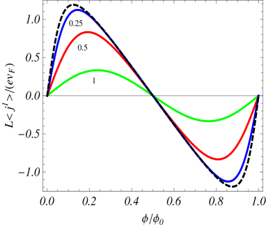
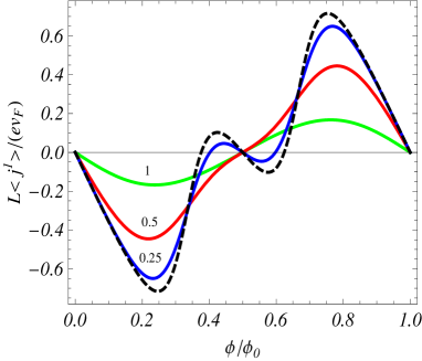
Figure 5: Current density as a function of the magnetic flux for $\alpha=0$ (left panel) and $\alpha=1/3$ (right panel). The graphs are plotted for $x_{c}=0.5$ and the curves are labelled with the value of $TN_{c}/\gamma_{F}$.

6.2 FC and the current in cylindrical nanotubes

The contributions from separate valleys to the FC and the current density along the compact dimension for a cylindrical nanotube are obtained specifying in the formulas above $p=q=1$ and $N=2$. Combining these contributions in accordance with Eq. (5.5) and adding a factor 2 corresponding to the spin states $s=\pm 1$, by taking into account Eq. (6.2), for the FC we get the following representations:

$$\left\langle\bar{\psi}\psi\right\rangle=-\frac{4x_{c}}{\pi L^{2}}\sum_{n=1}^{\infty}\bigg{[}\frac{\sin(2\pi n\alpha)}{ne^{nx_{c}}}\sin(2\pi n\phi/\phi_{0})+(-1)^{n}\sum_{l=-\infty}^{+\infty}\sum_{j=\pm 1}jK_{0}(nb_{l}^{(j)}y_{c})\bigg{]},$$ (6.14)

with the same notations as in Eq. (6.3), and

$$\left\langle\bar{\psi}\psi\right\rangle=-\frac{8x_{c}}{\pi L^{2}}\sideset{}{{}^{\prime}}{\sum}_{n=0}^{\infty}(-1)^{n}\sum_{l=1}^{\infty}\sin(2\pi l\alpha)\sin(2\pi l\phi/\phi_{0})\frac{e^{-x_{c}\sqrt{l^{2}+n^{2}y_{c}^{2}}}}{\sqrt{l^{2}+n^{2}y_{c}^{2}}}.$$ (6.15)

At high temperatures one has the asymptotic behavior

$$\left\langle\bar{\psi}\psi\right\rangle\approx-\frac{16x_{c}\sin(2\pi l\alpha)}{\pi L^{2}\sqrt{2y_{c}}}\sin(2\pi l\phi/\phi_{0})e^{-\pi/y_{c}}\ .$$ (6.16)

For single-walled cylindrical nanotubes $N_{c}\sim 10$ and for the characteristic energy scale one has $\gamma_{F}/N_{c}\sim 0.2\,\mathrm{eV}$. The corresponding characteristic temperature $T_{c}=\gamma_{F}/(N_{c}k_{\mathrm{B}})\approx 3\cdot 10^{3}\,\mathrm{K}$. For $T\ll k_{\mathrm{B}}T_{c}$, the finite temperature corrections are small and the contribution of the vacuum expectation value dominates. In figure 6 we have plotted the FC, given by Eq. (6.14), as a function of the magnetic flux for $\alpha=1/3$ and $x_{c}=0.5$. The numbers near the curves correspond to the value of $TN_{c}/\gamma_{F}$.

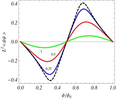
Figure 6: FC in a carbon nanotube as a function of the magnetic flux for $\alpha=1/3$ and $x_{c}=0.5$. The numbers near the curves correspond to the values of $TN_{c}/\gamma_{F}$.

Now let us consider the current density. By summing the contributions coming from two separate valleys with opposite signs of $\alpha$, again, we find two representations:

$$\left\langle j^{2}\right\rangle=\frac{4ev_{F}}{\pi L^{2}}\sum_{n=1}^{\infty}\bigg{[}\cos(2\pi n\alpha)\sin(2\pi n\phi/\phi_{0})\frac{1+nx_{c}}{n^{2}e^{nx_{c}}}-(-1)^{n}\sum_{l=-\infty}^{+\infty}\sum_{j=\pm 1}\kappa_{l}^{(j)}K_{0}(nb_{l}^{(j)}y_{c})\bigg{]},$$ (6.17)

and

$$\left\langle j^{2}\right\rangle=\frac{8ev_{F}}{\pi L^{2}}\sideset{}{{}^{\prime}}{\sum}_{n=0}^{\infty}(-1)^{n}\sum_{l=1}^{\infty}l\sin(2\pi l\phi/\phi_{0})\frac{\cos(2\pi l\alpha)(1+x_{c}\sqrt{l^{2}+n^{2}y_{c}^{2}})}{(l^{2}+n^{2}y_{c}^{2})^{3/2}e^{x_{c}\sqrt{l^{2}+n^{2}y_{c}^{2}}}}.$$ (6.18)

In the absence of a gap energy one has $x_{c}=0$, and in Eq. (6.17) we take $b=|\kappa_{l}^{(j)}|$. At high temperatures the current density is exponentially suppressed:

$$\left\langle j^{2}\right\rangle\approx\frac{16e\cos(2\pi n\alpha)}{\sqrt{2}L^{2}y_{c}^{3/2}}\sin(2\pi n\phi/\phi_{0})e^{-\pi/y_{c}}\ .$$ (6.19)

In figure 7 we displayed the current density, in units of $ev_{F}/L$, as a function of the magnetic flux for $\alpha=0$ (left panel) and $\alpha=1/3$ (right panel) with fixed value of the gap corresponding to $x_{c}=0.5$. The numbers near the curves correspond to the values of $TN_{c}/\gamma_{F}$.

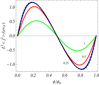
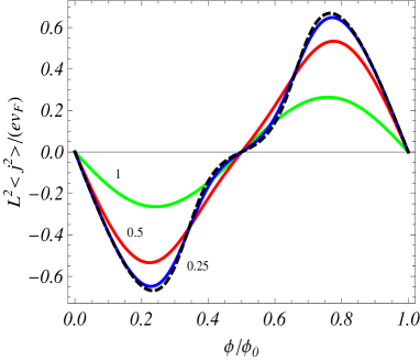
Figure 7: Current density along the compact dimension of a cylindrical nanotube as a function of the magnetic flux for $\alpha=0$ (left panel) and $\alpha=1/3$ (right panel). The graphs are plotted for $x_{c}=0.5$ and the numbers near the curves correspond to the values of $TN_{c}/\gamma_{F}$.

7 Conclusion

In this paper we have considered the combined effects of finite temperature and nontrivial topology on the FC and on the expectation values of charge and current densities for a massive fermionic field. Along compact dimensions, quasiperiodicity conditions (2.3) are imposed with arbitrary phases $\alpha_{l}$. Twisted and untwisted periodicity conditions, most often discussed in the literature, are special cases. In addition, we have assumed the presence of a constant gauge field which gives rise to Aharonov-Bohm-like effects on the expectation values. The effects of nontrivial phases in the boundary conditions and of the gauge field appear in the form of the combination $\tilde{\alpha}_{l}$, given by Eq. (2.24).

Under the condition $\left|\mu\right|<\varepsilon_{0}$, with $\varepsilon_{0}$ being the lowest energy in the energy spectrum of a fermionic particle (see Eq. (2.25)), the FC is given by Eq. (2.29), where $\left\langle\bar{\psi}\psi\right\rangle_{0}$ is the FC at zero temperatures and the second term on the right presents the finite temperature contribution. The FC is an even periodic function of $\tilde{\alpha}_{l}$ with the period equal to unity. In particular, it is a periodic function of the fluxes enclosed by compact dimensions with the period equal to the flux quantum. As a limiting case, from the general result we have derived the expression for the FC in the topologically trivial Minkowski spacetime, Eq. (2.31). If the length of one of the compact dimensions, say the $l$th dimension, is much smaller than the other length scales, the behavior of the FC crucially depends on the value of the parameter $\tilde{\alpha}_{l}$. Assuming that $|\tilde{\alpha}_{l}|<1/2$, for $\tilde{\alpha}_{l}\neq 0$ and for small values of $L_{l}$, the FC is suppressed by the factor $e^{-2\pi|\tilde{\alpha}_{l}|\beta/L_{l}}$. In the case $\tilde{\alpha}_{l}=0$, to the leading order the FC coincides with $N\left\langle\bar{\psi}\psi\right\rangle_{(p,q-1)}/(N_{D-1}L_{l})$, where $\left\langle\bar{\psi}\psi\right\rangle_{(p,q-1)}$ is the FC in the $(D-1)$-dimensional space of topology $R^{p}\times(S^{1})^{q-1}$. At low temperatures, the thermal corrections are suppressed by the factor $e^{-(\varepsilon_{0}-|\mu|)/T}$ (see Eq. (2.32)).

An alternative expression for the FC, Eq. (2.43), is obtained by using the analytic continuation of the generalized zeta function (2.37) provided by the Chowla-Selberg formula. A representation of the FC, Eq. (2.47), convenient in the investigation of the high temperature limit is obtained from Eq. (2.43) with the help of formula (2.46). At high temperatures, the dominant contribution comes from the terms with $n=0$ and $n=-1$ and the effects induced by the nontrivial topology are suppressed by the factor $e^{-\pi TL_{\mathrm{min}}}$, with $L_{\mathrm{min}}$ being the smallest length of the compact dimensions. In the high-temperature expansion of the FC, the leading terms coincides with that for the FC in the topologically trivial Minkowski spacetime with the asymptotic behavior given by Eq. (2.49). The representation of the FC, Eq. (2.55), containing more detailed explicit information, is obtained by applying a variant of the Abel-Plana summation formula (2.50). The second term in the right-hand side of Eq. (2.55) presents the part in the FC induced by the compactification of the $l$-th dimension. This information is not explicit in the previous two representations.

In the case $|\mu|>$ $\varepsilon_{0}$, assuming that $\mu>0$, the expression for the finite temperature part in the FC coming from the antiparticles remains the same, whereas in the part coming from the particles the spectral ranges $\varepsilon_{\mathbf{n}_{q}}\leqslant\varepsilon_{\mathbf{n}_{q}^{(0)}}$ and $\varepsilon_{\mathbf{n}_{q}}>\varepsilon_{\mathbf{n}_{q}^{(0)}}$ should be treated separately and the expression for the FC takes the form (2.58). Now, at zero temperature one has Eq. (2.59), where the second contribution in the right-hand side comes from the particles which occupy the states with $\varepsilon_{\mathbf{n}_{q}}<\mu$. At high temperatures, the leading term in the asymptotic expression for the FC remains the same, and it coincides with that in the topologically trivial Minkowski spacetime.

The expectation value of the charge density is investigated in Section 3. In the case $\left|\mu\right|<\varepsilon_{0}$, the zero temperature charge density vanishes, and the effects induced by the finite temperature are given by Eq. (3.7). The charge density is an even periodic function of the phases $\tilde{\alpha}_{l}$ with the period equal to unity. Besides, it is an odd function of the chemical potential $\mu$. For large values of the lengths of compact dimensions, in the leading order we recover the result for the topologically trivial Minkowski bulk, Eq. (3.8). At low temperatures the induced charge is exponentially small (see Eq. (3.9)). An equivalent representation for the charge density, Eq. (3.13), is obtained by making use of the related zeta function analytic continuation. At high temperatures the part in the charge density coming from the nontrivial topology is exponentially suppressed, and the leading term in the asymptotic expansion is given by the Minkowskian part, Eq. (3.15). Besides, another representation for the charge density, Eq. (3.16), is obtained by using the Abel-Plana formula. This representation separates the part due to the compactification of the $l$th compact dimension.

For $\left|\mu\right|>\varepsilon_{0}$ and assuming that $\mu>0$, the contribution to the charge density coming from antiparticles remain the same, and the total charge density is given by Eq. (3.17) (or equivalently by Eq. (3.20)). In this case the charge density at zero temperature is presented as Eq. (3.18). The latter is related to the number of states with the energies smaller than $|\mu|$ by a simple formula $\left\langle j^{0}\right\rangle_{T=0}=e\mathcal{N}_{\leqslant\mu}$. For a fixed value of the charge, the formulas for the charge density determine the chemical potential as a function of the charge, the temperature and the volume of the compact subspace. At high temperatures this function decays with the leading term (3.21). Decreasing the temperature, the chemical potential increases and its value at the zero temperature is determined by Eq. (3.18).

An interesting effect induced by the nontrivial topology is the appearance of the nonzero current density along compact dimensions. The current density along the $\nu$-th compact dimension, given by Eq. (4.4) for $\left|\mu\right|<\varepsilon_{0}$, is an even periodic function of the phases $\tilde{\alpha}_{l}$, $l\neq\nu$, with the period equal to unity, and an odd periodic function of the phase $\tilde{\alpha}_{\nu}$. In particular, the current density vanishes for twisted and untwisted fields in the absence of the gauge field. The current density is an even function of the chemical potential. At low temperatures it coincides with the corresponding result al zero temperature, given by Eq. (4.16), for $\left|\mu\right|<\varepsilon_{0}$, up to exponentially small terms. At high temperatures, the thermal corrections to the current density along the $\nu$th compact dimension are suppressed by the factor $e^{-\pi TL_{\nu}}$. This behavior is in sharp contrast with the high-temperature asymptotic of the current density in the case of a scalar field. For the latter, the current density linearly grows with the temperature. For $\mu>\varepsilon_{0}$, the contribution of the particles to the current density with the energies $\varepsilon_{\mathbf{n}_{q}}<\mu$ should be considered separately and the corresponding expression takes the form (4.22). Now the current density at zero temperature receives the contributions from both virtual and real particles. The latter is given by the second term in the right-hand side of Eq. (4.23). The asymptotic behavior at high temperatures remains the same. We have also investigated the current density along compact dimensions for a fixed value of the charge. A numerical example for a $D=3$ model with a single compact dimension is presented in figure 3.

For odd spacetime dimensions, with an irreducible representation of the Clifford algebra, the mass term breaks $C$-invariance in $D=4n$, $P$-invariance in $D=4n,4n+2$, and $T$-invariance in $D=4n+2$. In the absence of magnetic fields, these symmetries are restored in the model with two fermionic fields realizing two inequivalent representations of the Clifford algebra. These two fields can be combined in a single $2N$-component spinor with the Lagrangian density (5.4). The respective FC and the current densities are obtained by combining the corresponding results for the upper and lower components of this spinor in the form of Eq. (5.5). As an application of the general results we have considered the $D=2$ model used for the effective field theoretical description of low-energy degrees of freedom of the electrons in a graphene sheet. For carbon nanotubes the corresponding topology is $R^{1}\times S^{1}$. Depending on the chiral vector of the nanotube, for the phases in the quasiperiodicity conditions one has $\alpha_{l}=0,\pm 1/3$, and the phases have opposite signs for the upper and lower components of the 4-spinor. Compactifying the direction along the nanotube axis, one gets toroidal carbon nanotubes with the topology of a two-torus for the effective Dirac theory. As a simple model of a toroidal nanotube, we have considered a one-dimensional ring. For simplicity, in both cases of cylindrical and toroidal topologies we have assumed the zero chemical potential. In this case the charge density vanishes. On the base of the formulas for general $D$, the generalization of the corresponding expressions of the FC and current density in nanotubes for the case of a nonzero chemical potential is straightforward.

References

- [1] A. Linde, JCAP 0410, 004 (2004).
- [2] G. D. Starkman, Classical Quantum Gravity 15, 2529 (1998); N. J. Cornish, D. N. Spergel, and G. D. Starkman, Classical Quantum Gravity 15, 2657 (1998).
- [3] V. P. Gusynin, S. G. Sharapov, and J. P. Carbotte, Int. J. Mod. Phys. B 21, 4611 (2007); A. H. Castro Neto, F. Guinea, N. M. R. Peres, K. S. Novoselov, and A. K. Geim, Rev. Mod. Phys. 81, 109 (2009).
- [4] V.M. Mostepanenko and N.N. Trunov, The Casimir Effect and Its Applications (Clarendon, Oxford, 1997); K.A. Milton, The Casimir Effect: Physical Manifestation of Zero-Point Energy (World Scientific, Singapore, 2002); M. Bordag, G.L. Klimchitskaya, U. Mohideen, and V.M. Mostepanenko, Advances in the Casimir Effect (Oxford University Press, Oxford, 2009); Lecture Notes in Physics: Casimir Physics, Vol. 834, edited by D. Dalvit, P. Milonni, D. Roberts, and F. da Rosa (Springer, Berlin, 2011).
- [5] M.J. Duff, B.E.W. Nilsson, and C.N. Pope, Phys. Rep. 130, 1 (1986); R. Camporesi, Phys. Rep. 196, 1 (1990); A.A. Bytsenko, G. Cognola, L. Vanzo, and S. Zerbini, Phys. Rep. 266, 1 (1996); A.A. Bytsenko, G. Cognola, E. Elizalde, V. Moretti, and S. Zerbini, Analytic Aspects of Quantum Fields (World Scientific, Singapore, 2003); E. Elizalde, Ten Physical Applications of Spectral Zeta Functions (Springer Verlag, 2012).
- [6] E. Elizalde, Phys. Lett. B 516, 143 (2001); C.L. Gardner, Phys. Lett. B 524, 21 (2002); K.A. Milton, Grav. Cosmol. 9, 66 (2003); A.A. Saharian, Phys. Rev. D 70, 064026 (2004); E. Elizalde, J. Phys. A 39, 6299 (2006); A.A. Saharian, Phys. Rev. D 74, 124009 (2006); B. Green and J. Levin, JHEP 0711, 096 (2007); P. Burikham, A. Chatrabhuti, P. Patcharamaneepakorn, and K. Pimsamarn, JHEP 0807, 013 (2008); P. Chen, Nucl. Phys. B (Proc. Suppl.) 173, s8 (2009).
- [7] J. S. Dowker and R. Critchley, J. Phys. A 9, 535 (1976); R. Banach and J. S. Dowker, J. Phys. A 12, 2545 (1979); B.S. DeWitt, C. F. Hart, and C. J. Isham, Physica (Amsterdam) 96A, 197 (1979); S.G. Mamayev and N. N. Trunov, Russ. Phys. J. 22, 766 (1979); 23, 551 (1980); L. H. Ford, Phys. Rev. D 21, 933 (1980); J. Ambjørn and S. Wolfram, Ann. Phys. (N.Y.) 147, 1 (1983); S.G. Mamayev and V. M. Mostepanenko, in Proceedings of the Third Seminar on Quantum Gravity (World Scientific, Singapore, 1985); Yu. P. Goncharov and A. A. Bytsenko, Phys. Lett. B 160, 385 (1985); Nucl. Phys. B 271, 726 (1986); Classical Quantum Gravity 4, 555 (1987); E. Elizalde, Z. Phys. C 44, 471 (1989); E. Ponton and E. Poppitz, J. High Energy Phys. 06 (2001) 019; H. Queiroz, J. C. da Silva, F. C. Khanna, J. M. C. Malbouisson, M. Revzen, and A. E. Santana, Ann. Phys. (Leipzig) 317, 220 (2005); S. Bellucci and A. A. Saharian, Phys. Rev. D 80, 105003 (2009); A. A. Saharian and A. L. Mkhitaryan, Eur. Phys. J. C 66, 295 (2010).
- [8] S. Bellucci and A.A. Saharian, Phys. Rev. D 79, 085019 (2009).
- [9] A. A. Saharian and M. R. Setare, Phys. Lett. B 659, 367 (2008); S. Bellucci and A. A. Saharian, Phys. Rev. D 77, 124010 (2008).
- [10] A. A. Saharian, Classical Quantum Gravity 25, 165012 (2008); E.R. Bezerra de Mello and A. A. Saharian, J. High Energy Phys. 12 (2008) 081.
- [11] S. Bellucci and A.A. Saharian, Phys. Rev. D 82, 065011 (2010).
- [12] S. Bellucci and A.A. Saharian, Phys. Rev. D 87, 025005 (2013).
- [13] S. Bellucci, A. A. Saharian, and H. A. Nersisyan, Phys. Rev. D 88, 024028 (2013).
- [14] L. Sriramkumar, Class. Quantum Grav. 18, 1015 (2001); Yu.A. Sitenko and N.D. Vlasii, Class. Quantum Grav. 26, 195009 (2009); E.R. Bezerra de Mello, V.B. Bezerra, A.A. Saharian, and V.M. Bardeghyan, Phys. Rev. D 82, 085033 (2010); E. R. Bezerra de Mello and A. A. Saharian, Eur. Phys. J. C., 73, 2532 (2013).
- [15] E. R. Bezerra de Mello and A. A. Saharian, Phys. Rev. D 87, 045015 (2013).
- [16] M.B. Altaie and J.S. Dowker, Phys. Rev. D 18, 3557 (1978); M.A. Rubin and B.D. Roth, Nucl. Phys. B 226, 444 (1983); F.S. Accetta, Phys. Rev. D 34, 1798 (1986); K. Shiraishi, Prog. Theor. Phys. 77, 975 (1987); K. Shiraishi, Prog. Theor. Phys. 77, 1253 (1987); A.A. Bytsenko, L. Vanzo, and S. Zerbini, Mod. Phys. Lett. A 7, 2669 (1992); H. Kleinert and A. Zhuk, Theor. Math. Phys. 108, 1236 (1996); A. Zhuk and H. Kleinert, Theor. Math. Phys. 109, 1483 (1996); I. Brevik, A.A. Bytsenko, A.E. Goncalves, and F.L. Williams, J. Phys. A: Math. Gen. 31, 4437 (1998); I. Brevik, K.A. Milton, and S.D. Odintsov, Ann. Phys. 302, 120 (2002); A.P.C. Malbouisson, J.M.C. Malbouisson, and A.E. Santana, Nucl. Phys. B 631, 83 (2002); H. Queiroz, J.C. da Silva, F.C. Khanna, J.M.C. Malbouisson, M. Revzen, and A.E. Santana, Ann. Phys. 317, 220 (2005); V.B. Bezerra, G.L. Klimchitskaya, V.M. Mostepanenko, and C. Romero, Phys. Rev. D 83, 104042 (2011); V.B. Bezerra, V.M. Mostepanenko, H. F. Mota, and C. Romero, Phys. Rev. D 84, 104025 (2011); F.C. Khanna, A.P.C. Malbouisson, J.M.C. Malbouisson, and A.E. Santana, Ann. Phys. 326, 2634 (2011).
- [17] J.S. Dowker, Class. Quantum Grav. 1, 359 (1984).
- [18] R. Camporesi, Clas. Quantum Grav. 8, 529 (1991).
- [19] A. Actor, Class. Quantum Grav. 7, 663 (1990); K. Kirsten, J. Phys. A 26, 2421 (1993).
- [20] E. Elizalde, S.D. Odintsov, A. Romeo, A.A. Bytsenko, and S. Zerbini, Zeta Regularization Techniques with Applications (World Scientific, Singapore, 1994); K. Kirsten, Spectral Functions in Mathematics and Physics (CRC Press, Boca Raton, FL, 2001).
- [21] E. Elizalde, Commun. Math. Phys. 198, 83 (1998); E. Elizalde, J. Phys. A 34, 3025 (2001).
- [22] E.R. Bezerra de Mello and A.A. Saharian, Phys. Rev. D 78, 045021 (2008).
- [23] K. Shimizu, Prog. Theor. Phys. 74, 610 (1985).
- [24] R. Saito, G. Dresselhaus, and M. S. Dresselhaus, Physical Properties of Carbon Nanotubes (Imperial College Press, London, 1998); J.-C. Charlier, X. Blase, and S. Roche, Rev. Mod. Phys. 79, 677 (2007).
- [25] S. G. Sharapov, V. P. Gusynin, and H. Beck, Phys. Rev. B 69, 075104 (2004); V. P. Gusynin and S. G. Sharapov, Phys. Rev. B 73, 245411 (2006).
- [26] T. Ando, J. Phys. Soc. Jpn. 74, 777 (2005).
- [27] J. Liu et al., Nature 385, 780 (1997); M. Ahlskog et al., Chem. Phys. Lett. 300, 202 (1999); M. Sano et al., Science 293, 1299 (2001); R. Martel et al., Nature 398, 299 (1999).
- [28] M.F. Lin and D.S. Chuu, Phys. Rev. B 57, 6731 (1998); M. Marganska and M. Szopa, Acta Phys. Pol. B 32, 427 (2001); S. Latil, S. Roche, and A. Rubio, Phys. Rev. B 67, 165420 (2003); R. B. Chen et al., Carbon 42, 2837 (2004); K. Sasaki and Y. Kawazoe, Prog. Theor. Phys. 112, 369 (2004); Z. Zhang, J. Yuan, M. Qiu, J. Peng, and F. Xiao, J. Appl. Phys. 99, 104311 (2006); N. Xu, J.W. Ding, H.B. Chen, and M.M. Ma, Eur. Phys. J. B 67, 71 (2009).
- [29] H. Bluhm et al., Phys. Rev. Lett. 102, 136802 (2009); A.C. Bleszynski-Jayich et al., Science 326, 272 (2009).