Generalized Taylor-Duffy Method for Efficient Evaluation of Galerkin Integrals in Boundary-Element Method Computations

Abstract

We present a generic technique, automated by computer-algebra systems and available as open-source software [1], for efficient numerical evaluation of a large family of singular and nonsingular 4-dimensional integrals over triangle-product domains, such as those arising in the boundary-element method (BEM) of computational electromagnetism. Previously, practical implementation of BEM solvers often required the aggregation of multiple disparate integral-evaluation schemes [2, 3, 4, 5, 6, 7, 8, 9, 10, 11, 12, 13, 14, 15, 16] in order to treat all of the distinct types of integrals needed for a given BEM formulation; in contrast, our technique allows many different types of integrals to be handled by the same algorithm and the same code implementation. Our method is a significant generalization of the Taylor–Duffy approach [2, 3], which was originally presented for just a single type of integrand; in addition to generalizing this technique to a broad class of integrands, we also achieve a significant improvement in its efficiency by showing how the dimension of the final numerical integral may often reduced by one. In particular, if $n$ is the number of common vertices between the two triangles, in many cases we can reduce the dimension of the integral from $4-n$ to $3-n$, obtaining a closed-form analytical result for $n=3$ (the common-triangle case).

I Introduction

The application of boundary-element methods {BEM [17, 18], also known as the method of moments (MOM)} to surfaces discretized into triangular elements commonly requires evaluating four-dimensional integrals over triangle-product domains of the form

$$\mathcal{I}=\int_{\mathcal{T}}\,d\mathbf{x}\,\int_{\mathcal{T}^{\prime}}\,d\mathbf{x}^{\prime}\,P\big{(}\mathbf{x},\mathbf{x}^{\prime}\big{)}K\big{(}|\mathbf{x}-\mathbf{x}^{\prime}|\big{)}$$ (1)

where $P$ is a polynomial, $K(r)$ is a kernel function which may be singular at $r=0$, and $\mathcal{T},\mathcal{T}^{\prime}$ are flat triangles; we will here be concerned with the case in which $\mathcal{T},\mathcal{T}^{\prime}$ have one or more common vertices. Methods for efficient and accurate evaluation of such integrals have been extensively researched; among the most popular strategies are singularity subtraction (SS) [4, 5, 6], singularity cancellation (SC) [7, 8, 9, 10, 11], and fully-numerical schemes [12, 13]. (Strategies have also been proposed to handle the near-singular case in which $\mathcal{T},\mathcal{T}^{\prime}$ have vertices which are nearly but not precisely coincident [19, 20]; we do not address that case here.) Particularly interesting among SC methods is the scheme proposed by Taylor [2] following earlier ideas of Duffy [3] (see also Refs. [14, 15, 16]); we will refer to the method of Ref. 2 as the the “Taylor-Duffy method” (TDM). This method considered the specific kernel $K^{\hbox{\scriptsize{Helmholtz}}}(r)=\frac{e^{ikr}}{4\pi r}$ and a specific linear polynomial $P^{\hbox{\scriptsize{linear}}}$ and reduced the singular 4-dimensional integral (1) to a nonsingular $(4-n)$-dimensional integral (where $n\in\{1,2,3\}$ is the number of vertices common to $\mathcal{T},\mathcal{T}^{\prime}$) with a complicated integrand obtained by performing various manipulations on $K^{\hbox{\scriptsize{Helmholtz}}}$ and $P^{\hbox{\scriptsize{linear}}}$. The reduced integral is then evaluated numerically by simple cubature methods.

Our first objective is to show that the TDM may be generalized to handle a significantly broader class of integrand functions. Whereas Ref. 2 addressed the specific case of the Helmholtz kernel combined with constant or linear factors, the master formulas we present [equations (2) in Section II] are nonsingular reduced-dimensional versions of (1) that apply to a broad family of kernels $K$ combined with arbitrary polynomials $P$. Our master formulas (2) involve new functions $\mathcal{K}$ and $\mathcal{P}$ derived from $K$ and $P$ in (1) by procedures, discussed in the main text and Appendices, that abstract and generalize the techniques of Ref. 2.

We next extend the TDM by showing that, for some kernels—notably including the “$r-$power” kernel $K(r)=r^{p}$ for integer $p$—the reduction of dimensionality effected by the TDM may be carried one dimension further, so that the original 4-dimensional integral is converted into a $(3-n)$-dimensional integral [equations (5) in Section III]. In particular, in the common-triangle case $(n=3)$, we obtain a closed-form analytical solution of the full 4-dimensional integral (1). This result encompasses and generalizes existing results [21, 22] for closed-form evaluations of the four-dimensional integral for certain special $P$ and $K$ functions.

A characteristic feature of many published strategies for evaluating integrals of the form (1) is that they depend on specific choices of the $P$ and $K$ functions, with (in particular) each new type of kernel understood to necessitate new computational strategies. In practical implementations this can lead to cluttered codes, requiring multiple distinct modules for evaluating the integrals needed for distinct BEM formulations. The technique we propose here alleviates this difficulty. Indeed, as we discuss in Section V, the flexibility of our generalized TDM allows the same basic code {$\sim$1,500 lines of C++ (not including general-purpose utility libraries), available for download as free open-source software [1]} to handle all singular integrals arising in several popular BEM formulations. Although separate techniques for computing these integrals have been published before, the novelty of our approach is to attack many different integrals with the same algorithm and the same code implementation.

Of course, the efficiency and generality of the TDM reduction do not come for free: the cost is that the reduction process—specifically, the procedure by which the original polynomial $P$ in (1) is converted into new polynomials $\mathcal{P}$ that enter the master formulas (2) and (5)—is tedious and error-prone if carried out by hand. To alleviate this difficulty, we have developed a computer-algebra technique for automating this conversion (Section IV); our procedure inputs the coefficients of $P$ and emits code for computing $\mathcal{P}$, which may be directly incorporated into routines for numerical evaluation of the integrands of the reduced integrals (2) or (5).

Figure 1: The basic TDM for once-integrable kernels reduces the original integral (1) to a 1-, 2-, or 3-dimensional integral in the (a) common-triangle, (b) common-edge, and (c) common-vertex cases respectively. (Note that this is an exact, not approximate, reduction.) The $\mathcal{P}$ and $\mathcal{K}$ functions in the integrands are derived from the $P$ and $K$ functions in the original integral (1) by procedures discussed in the main text.

The TDM reduces the 4-dimensional integral (1) to a lower-dimensional integral which is evaluated by numerical cubature. How smooth is the reduced integrand, and how rapidly does the cubature converge with the number of integrand samples? These questions are addressed in Section VI, where we plot integrands and convergence rates for the reduced integrals resulting from applying the generalized TDM to a number of practically relevant cases of (1). We show that—notwithstanding the presence of singularities in the original integral or geometric irregularities in the panel pair—the reduced integrand is typically a smooth, well-behaved function which succumbs readily to straightforward numerical cubature.

Although the TDM is an SC scheme, it has useful application to SS schemes. In such methods one subtracts the first few terms from the small-$r$ expansion of the Helmholtz kernels; the non-singular integral involving the subtracted kernel is evaluated by simple numerical cubature, but the integrals involving the singular terms must be evaluated by other means. In Section VII we note that these are just another type of singular integral of the form (1), whereupon they may again be evaluated using the same generalized TDM code—and, moreover, because the kernel in these integrals is just the “$r$-power” kernel $K(r)=r^{p}$, the improved TDM reduction discussed in Section III is available. We compare the efficiency of the unadorned TDM to a combined TDM/SS method and note that the latter is particularly effective for broadband studies of the same structure at many different frequencies.

Finally, in Section VIII we note a curious property of the Helmholtz kernel in the short-wavelength limit: as $k\to\infty$: this kernel becomes “twice-integrable” (a notion discussed below), and the accelerated TDM scheme of Section III becomes available. In particular, in the common-triangle case, the full four-dimensional integral (1) with $K(r)=\frac{e^{ikr}}{4\pi r}$ and arbitrary polynomial $P$ may be evaluated in closed analytical form in this limit.

Our conclusions are presented in Section IX, and a number of technical details are relegated to the Appendices. A free, open-source software implementation of the method presented in this paper is available online [1].

II Master Formulas for the Generalized Taylor-Duffy Method

Ref. 2 considered the integral (1) for specific choices of $K$ and $P$—namely, the Helmholtz kernel $K=K^{\hbox{\scriptsize{Helmholtz}}}$ and a certain linear polynomial $P=P^{\hbox{\scriptsize{linear}}}$—and showed that the singular 4-dimensional integral could be reduced to a nonsingular lower-dimensional integral with a complicated integrand obtained by performing various manipulations on $K^{\hbox{\scriptsize{Helmholtz}}}$ and $P^{\hbox{\scriptsize{linear}}}.$ The dimension of the reduced integral is $4-n$, where $n$ is the number of common vertices between $\mathcal{T},\mathcal{T}^{\prime}$. The objective of this section is to abstract and generalize the procedure of Ref. 2 to handle integrals of the form (1) for general $K$ and $P$ functions.

(More specifically—as discussed in Ref. 2— the reduction proceeds by dividing the original four-dimensional region of integration into multiple subregions, introducing appropriate variable transformations for each subregion that allow one or more integrations to be performed analytically, then summing the results for all subregions to obtain a single lower-dimensional integral. A detailed review of this procedure, using the generalized notation of this paper, may be found online in the documentation for our open-source code [1].)

The result is equation (2) at the top of the following page; here integrals (2){a,b,c} are nonsingular integrals which evaluate to the same result as integral (1) for the common-triangle $(n=3)$, common-edge $(n=2)$, and common-vertex $(n=1)$ cases, respectively. In particular, equation (2)a may be understood as a generalized version of equation (46) in Ref. 2. In the integrals of equation (2),

• The domain of integration in each integral is fixed (it is the unit {interval, square, cube} for the {CT, CE, CV} case) independent of $P$, $K$, and the triangles $\{\mathcal{T},\mathcal{T}^{\prime}\}$. Thus a numerical implementation need only furnish cubature rules for these three fixed domains; there is no need to construct custom-designed cubature rules for particular triangles or integrand functions.

• The $d$ index runs over subregions into which the original dimensional integration domain is divided; there are $\{3,6,2\}$ subregions for the {CT, CE, CV} cases.

• For each subregion $d$, the $X_{d}$ functions are “reduced distance” functions for that subregion. $X_{d}(\{y_{i}\})$ is the square root of a second-degree polynomial in the $y_{i}$ variables, whose coefficients depend on the geometrical parameters of the two triangles. (Explicit expressions are given in Appendix A.) Note that the division into subregions, and the $X_{d}$ functions, are independent of the specific $P$ and $K$ functions in the original integrand.

• For each subregion $d$ and each integer $n$, the functions $\mathcal{P}_{dn}(y_{i})$ are polynomials derived from the original polynomial $P(\mathbf{x},\mathbf{x}^{\prime})$ in (1). For a given $P(\mathbf{x},\mathbf{x}^{\prime}),$ the derived polynomials $\mathcal{P}_{dn}$ are only nonzero for certain integers $n$; this defines the limits of the $n$ summations in (2). The procedure for obtaining $\mathcal{P}$ from $P$ is discussed in Section IV and Appendix A.

• For each integer $n$, the function $\mathcal{K}_{n}$ is obtained from the $K$ kernel as follows:

  $$\mathcal{K}_{n}(X)\equiv\int_{0}^{1}w^{n}K(wX)\,dw.$$ (3)

  For several kernels of interest, this integral may be evaluated explicitly to obtain a closed-form expression for $\mathcal{K}_{n}$. We will refer to such kernels as once-integrable. Appendix B tabulates the $\mathcal{K}_{n}$ functions for several once-integrable kernel functions. (In the following section we will introduce the further notion of twice-integrability.)

The key advantage of the TDM is that equation (3) isolates the integrable singularities in (1) into a one-dimensional integral which may be performed analytically. This not only reduces the dimension of the original integral (1), but also neutralizes its singularities, leaving behind a smooth integrand. (In the CT and CE cases, the dimension of the integral may be reduced further.) The remaining integrals (2), though complicated, are amenable to efficient evaluation by numerical cubature.

The extent to which the singularities of $K$ are regulated depends on the polynomial $P$. More specifically, if the original kernel $K(r)$ diverges for small $r$ like $r^{-L}$, then equation (3) will be finite only for $n\geq L$. As noted above, the range $[n^{\hbox{\scriptsize{min}}},n^{\hbox{\scriptsize{max}}}]$ of integers $n$ for which we need to compute (3) depends on the number of common vertices and on the polynomial $P$ (in particular, $n^{\hbox{\scriptsize{min}}}$ is greater for polynomials that vanish at $\mathbf{x}=\mathbf{x}^{\prime}$). For example, in the common-triangle case with polynomial $P\equiv 1$ one finds $n^{\hbox{\scriptsize{min}}}=1$; thus in this case we can integrate kernels $K(r)$ that behave for small $r$ like $1/r$, but not kernels that diverge like $1/r^{2}$ or faster. On the other hand, in the common-edge case with $P=P^{\hbox{\scriptsize{MFIE}}}$ (Section V) one finds $n^{\hbox{\scriptsize{min}}}=3$, allowing treatment of kernels with $1/r^{3}$ singularities such as $K^{\hbox{\scriptsize{MFIE}}}(r)=(ikr-1)\frac{e^{ikr}}{4\pi r^{3}}$.

III Improved TDM Formulas for Twice-Integrable Kernels

The TDM reduces the original 4-dimensional integral (1) to the $(4-n)$-dimensional integral (2) where $n\in\{1,2,3\}$ is the number of common vertices. In this section we show that, for certain kernel functions, it is possible to go further; when the kernel is twice-integrable, in a sense defined below, the original 4-dimensional integral is reduced to a $(3-n)$-dimensional integral. In particular, for the case $n=3$, the full 4-dimensional integral may be evaluated explicitly to yield a closed-form expression requiring no numerical integrations.

The master TDM formulas for twice-integrable kernels are equations (5) at the top of the following page, and their derivation is discussed below.

Twice-Integrable Kernels

Above we referred to a kernel function $K(r)$ as once integrable if it is possible to evaluate the integral (3) in closed form. For such kernels, we now introduce a further qualification: we refer to $K(r)$ as twice-integrable if it is possible to obtain closed-form expressions for the following two integrals involving the $\mathcal{K}$ function defined by (3):

$$\mathcal{J}_{n}(\alpha,\beta,\gamma) \equiv\int_{0}^{1}\mathcal{K}_{n}\Big{(}\alpha\sqrt{(y+\beta)^{2}+\gamma^{2}}\Big{)}\,dy$$ (4a)

$$\mathcal{L}_{n}(\alpha,\beta,\gamma) \equiv\int_{0}^{1}y\,\mathcal{K}_{n}\Big{(}\alpha\sqrt{(y+\beta)^{2}+\gamma^{2}}\Big{)}\,dy.$$ (4b)

In particular, the kernel $K(r)=r^{p}$ is twice-integrable for arbitrary integer powers $p$; moreover, in Section VIII we show that the Helmholtz kernels become twice-integrable in the limit $\text{Im }k\to\infty.$ (Expressions for $\mathcal{J}$ and $\mathcal{L}$ in all these cases are collected in Appendix B.)

Figure 2: The TDM for twice-integrable kernels reduces the original integral (1) to a 0-, 1-, or 2-dimensional integral in the (a) common-triangle, (b) common-edge, and (c) common-vertex cases respectively.

The TDM For Twice-Integrable Kernels

For twice-integrable kernels, the formulas (2) may be further simplified by analytically evaluating the innermost integral in each case. Thus, for the {CT, CE, CV} case, we analytically perform the $\{y_{1},y_{2},y_{3}\}$ integration.

We will consider here the case in which the $\mathcal{P}$ polynomials are of degree not greater than 1 in the innermost integration variable. (This condition is satisfied, in particular, for all but one of the eight distinct forms of the $P$ polynomials considered in Section V.) More general cases could be handled by extending the methods of this section.

The Common-Triangle Case

Given the above assumption on the degree of the $\mathcal{P}$ polynomials, we can write, in the common-triangle case,

$$\mathcal{P}^{\hbox{\tiny{CT}}}_{dn}(y)=\mathcal{P}^{\hbox{\tiny{CT}}}_{dn0}+y\mathcal{P}^{\hbox{\tiny{CT}}}_{dn1},$$ (6)

where $\mathcal{P}^{\hbox{\tiny{CT}}}_{dn0}$ and $\mathcal{P}^{\hbox{\tiny{CT}}}_{dn1}$ are just the constant and linear coefficients in the polynomial $\mathcal{P}^{\hbox{\tiny{CT}}}_{dn}(y)$. The Taylor-Duffy formula for the common-triangle case, equation (2a), then becomes

$$\mathcal{I}^{\hbox{\tiny{CT}}}=\sum_{d=1}^{3}\sum_{n}\bigg{\{} \mathcal{P}^{\hbox{\tiny{CT}}}_{dn0}\int_{0}^{1}dy\,\mathcal{K}_{n+1}\Big{(}X^{\hbox{\tiny{CT}}}_{d}(y)\Big{)}$$

$$\quad+\mathcal{P}^{\hbox{\tiny{CT}}}_{dn1}\,\int_{0}^{1}dy\,y\,\mathcal{K}_{n+1}\Big{(}X^{\hbox{\tiny{CT}}}_{d}(y)\Big{)}\bigg{\}}.$$ (7)

If we now write the reduced-distance function $X^{\hbox{\tiny{CT}}}_{d}(x)$ in the form (Appendix A)

$$X^{\hbox{\tiny{CT}}}_{d}(y)\equiv\alpha^{\hbox{\tiny{CT}}}_{d}\sqrt{(y+\beta^{\hbox{\tiny{CT}}}_{d})^{2}+(\gamma^{\hbox{\tiny{CT}}}_{d})^{2}}$$ (8)

(where $\alpha_{d},\beta_{d}$, and $\gamma_{d}$ are functions of the geometrical parameters such as triangle side lengths and areas) then we can immediately use equations (4) to evaluate the $y$ integrals in (7), obtaining an exact closed-form expression for the full 4-dimensional integral (1) in the common-triangle case. This is equation (5a).

We emphasize again that (5a) involves no further integrations, but is a closed-form expression for the full 4-dimensional integral in (1). Closed-form expressions for certain special cases of 4-dimensional triangle-product integrals in BEM schemes have appeared in the literature before [21, 22], but we believe equation (5a) to be the most general result available to date.

The Common-Edge and Common-Vertex Cases

We now proceed in exactly analogous fashion for the common-edge and common-vertex cases. We will show that, for twice-integrable kernels, the 2-dimensional and 3-dimensional integrals obtained via the usual TDM [equations (2b, 2c)] may be reduced to 1-dimensional and 2-dimensional integrals, respectively.

Because the $\mathcal{P}^{\hbox{\tiny{CE}}}$ and $\mathcal{P}^{\hbox{\tiny{CV}}}$ polynomials are (by assumption) not more than linear in the variables $y_{2}$ and $y_{3}$, respectively, we can write, in analogy to (6),

$$\mathcal{P}^{\hbox{\tiny{CE}}}_{dn}(y_{1},y_{2}) =\mathcal{P}^{\hbox{\tiny{CE}}}_{dn0}+y_{2}\mathcal{P}^{\hbox{\tiny{CE}}}_{dn1}$$ (9a)

$$\mathcal{P}^{\hbox{\tiny{CV}}}_{dn}(y_{1},y_{2},y_{3}) =\mathcal{P}^{\hbox{\tiny{CV}}}_{dn0}+y_{3}\mathcal{P}^{\hbox{\tiny{CV}}}_{dn1}$$ (9b)

where the ${\mathcal{P}}^{\hbox{\tiny{CE}}}_{dni}$ coefficients depend on $y_{1}$ in addition to the geometric parameters, while the ${\mathcal{P}}^{\hbox{\tiny{CV}}}_{dni}$ coefficients depend on $y_{1}$ and $y_{2}$ in addition to the geometric parameters.

Similarly, in analogy to (8), we write

$$X^{\hbox{\tiny{CE}}}_{d}(y_{1},y_{2})\equiv\alpha^{\hbox{\tiny{CE}}}_{d}\sqrt{(y_{2}+\beta^{\hbox{\tiny{CE}}}_{d})^{2}+(\gamma^{\hbox{\tiny{CE}}}_{d})^{2}}$$ (10a)

$$X^{\hbox{\tiny{CV}}}_{d}(y_{1},y_{2},y_{3})\equiv\alpha^{\hbox{\tiny{CV}}}_{d}\sqrt{(y_{3}+\beta^{\hbox{\tiny{CV}}}_{d})^{2}+(\gamma^{\hbox{\tiny{CV}}}_{d})^{2}}.$$ (10b)

where $\{\alpha,\beta,\gamma\}^{\hbox{\tiny{CE}}}_{d}$ depend on $y_{1}$ in addition to the geometric parameters, while $\{\alpha,\beta,\gamma\}^{\hbox{\tiny{CV}}}_{d}$ depend on $y_{1}$ and $y_{2}$ in addition to the geometric parameters.

Inserting (9) and (10) into (2b) and (2c) and evaluating the $y_{2}$ and $y_{3}$ integrals using (4), the original 4-dimensional integral (1) is then reduced to a 1-dimensional integral [equation (5b)] or a 2-dimensional integral [equation (5c)].

Thus, for twice-integrable kernels, the dimension of the numerical cubature needed to evaluate the original integral (1) is reduced by 1 compared to the case of once-integrable kernels.

Summary of Master TDM Formulas

For once-integrable kernel functions, the generalized TDM reduces the original 4-dimensional integral (1) to a $(4-n)$-dimensional integral, equation (2), where $n$ is the number of common vertices between the triangles.

For twice-integrable kernel functions, the generalized TDM reduces the original four-dimensional integral (1) to a $(3-n)$-dimensional integral, equation (5). In particular, in the common-triangle case $n=3$ we obtain a closed-form expression requiring no numerical integrations.

In addition to reducing the dimension of the integral, the TDM also performs the service of neutralizing singularities that may be present in the original four-dimensional integral, ensuring that the resulting integrals (2) or (5) are amenable to efficient evaluation by numerical cubature.

IV From $P$ to $\mathcal{P}$: Computer Algebra Techniques

The integrands of the Taylor-Duffy integrals (2) and (5) refer to polynomials $\mathcal{P}$ derived from the original polynomial $P$ appearing in the original integral (1). The procedure for obtaining $\mathcal{P}$ from $P$, summarized in equations (24), (26), and (28), is straightforward but tedious and error-prone if carried out by hand. For example, to derive the polynomials $\mathcal{P}_{dn}^{\hbox{\tiny{CT}}}$ in the common-triangle formulas (2a) and (5a), we must (a) define, for each subregion $d=1,2,3$, a new function $H_{d}(u_{1},u_{2})$ by evaluating a certain definite integral involving the $P$ polynomial, (b) evaluate the function $H$ at certain $w$-dependent arguments to obtain a polynomial in $w$, and then (c) identify the coefficients of $w^{n}$ in this polynomial as the $\mathcal{P}_{dn}^{\hbox{\tiny{CT}}}$ functions we seek. Moreover, we must repeat this procedure for each of the three subregions that enter the common-triangle case, and for the common-edge case we have six subregions. Clearly the process of reducing (1) to (2) or (5) is too complex a task to entrust to pencil-and-paper calculation.

However, the manipulations are ideally suited to evaluation by computer-algebra systems. For example, Figure 3 presents mathematica code that executes the procedure described above for deriving the $\mathcal{P}_{dn}^{\hbox{\tiny{CT}}}$ polynomials for one choice of $P(\mathbf{x},\mathbf{x}^{\prime})$ function (specifically, the polynomial named $P^{\hbox{\scriptsize{EFIE1}}}$ in Section V). Running this script yields the emission of machine-generated code for computing the $\mathcal{P}$ polynomials, and this code may be directly incorporated into a routine for computing the integrands of (2) or (5). (This and other computer-algebra codes for automating the procedures of this paper may be found together with our online open-source code distribution [1].)

(*****************************************)
(* P polynomial for the case             *)
(*  P(x,xp) = (x-Q) \cdot (xp - QP)      *)
(*****************************************)
P[Xi1_, Xi2_, Eta1_, Eta2_] :=           \
  Xi1*Eta1*A*A + Xi1*Eta2*AdB + Xi1*AdDP \
+ Xi2*Eta1*AdB + Xi2*Eta2*B*B + Xi2*BdDP \
+     Eta1*AdD +     Eta2*BdD +     DdDP;

(*****************************************)
(* region-dependent integration limits   *)
(* and u-functions, Eqs (21) and (23)    *)
(*****************************************)
u1[d_, y_]:=Switch[d, 1, 1, 2, y,   3, y];
u2[d_, y_]:=Switch[d, 1, y, 2, y-1, 3, 1];

Xi1Lower[d_, u1_, u2_]                   \
 := Switch[ d, 1, 0, 2, -u2, 3, u2-u1];
Xi1Upper[d_, u1_, u2_]                   \
 := 1-u1;
Xi2Lower[d_, u1_, u2_, Xi1_]             \
 := Switch[ d, 1, 0, 2, -u2, 3, 0];
Xi2Upper[d_, u1_, u2_, Xi1_]             \
  := Switch[ d, 1, Xi1, 2, Xi1,          \
                3, Xi1-(u1-u2)];

(*****************************************)
(* big H function, equation (22) *********)
(*****************************************)
H[u1_, u2_] :=                   \
 Integrate[                      \
  Integrate[                     \
    P[Xi1, Xi2, u1+Xi1, u2+Xi2]  \
  + P[u1+Xi1,u2+Xi2, Xi1, Xi2 ], \
   {Xi2Lower, 0, Xi2Upper }],    \
  {Xi1Lower, 0, Xi1Upper}];

(*****************************************)
(* \mathcal{P}_{dn} functions, eq. (24)  *)
(*****************************************)
wSeries =
 Series[ H[ w*u1[x], w*u2[x] ], {w,0,10} ];
P[n_,x_] := SeriesCoefficient[ wSeries, n];

Figure 3: mathematica code snippet that derives the $\mathcal{P}_{dn}^{\hbox{\tiny{CT}}}$ polynomials for a given $P(\mathbf{x},\mathbf{x}^{\prime})$ polynomial.

V Applications to BEM Formulations using Triangle-Supported Basis Functions

As noted in the Introduction, a key strength of our proposal is that the flexibility of our generalized TDM allows the same code to evaluate singular integrals for many different BEM formulations. Indeed, our implementation [1] ($\sim$1,500 lines of C++, not including utility libraries) suffices to handle all singular integrals arising in several popular BEM formulations: (a) electrostatics with triangle-pulse basis functions [23], (b) the electric-field integral equation (EFIE) with RWG basis functions [24], (c) the magnetic-field integral equation (MFIE) [25] or PMCHWT [26] formulations with RWG basis functions, (d) the n-Müller formulation with RWG basis functions [27]. [Moreover, in cases (b)–(d), the same code implementation evaluates not only the full-wave integrals but also the individual contributions to those integrals needed for singularity-subtraction schemes; this is discussed in Section VII.]

Of course, it is not a new result that singular integrals of the form (1) may be reduced to nonsingular lower-dimensional integrals; indeed, the reduction of case (b) was the subject of the original TDM paper [2], while numerous works have pursued other specialized approaches for the other cases [4, 5, 6, 7, 8, 9, 10, 11, 12, 13, 14, 15, 16]. The novelty of our contribution here is the observation that this proliferation of specialized approaches is in fact unnecessary; instead, all integrals arising in the four formulations above may be written in the form of equation (1), whereupon they may be reduced by the same generalized procedure to the same general reduced form [equations (2) or (7)] and then evaluated using the same generalized code. This is an advantage over the multiple distinct codes that would be required to implement each of the separate methods of the references cited above.

For reference, in this section we note the particular forms of the $P$ and $K$ functions needed to write Galerkin integrals for various BEM formulations in the form of equation (1). These $P$ and $K$ functions may then be transformed, via methods discussed elsewhere in this paper, into the $\mathcal{P}$ and $\mathcal{K}$ functions in the integrands of (2) and (7). Source-code implementations of these functions for all formulations mentioned above may be found in our open-source code [1].

Electrostatics with triangle-pulse functions

For electrostatic BEM formulations using “triangle-pulse” basis functions representing constant charge densities on flat triangular panels, we require the average over triangle $\mathcal{T}$ of the potential and/or normal electric field due to a constant charge density on $\mathcal{T}^{\prime}$. These are

$$\mathcal{I}^{\hbox{\scriptsize{ES1}}} =\int_{\mathcal{T}}\,\int_{\mathcal{T}^{\prime}}\,\frac{1}{4\pi|\mathbf{x}-\mathbf{x}^{\prime}|}\,\,d\mathbf{x}\,d\mathbf{x}^{\prime}$$ (11a)

$$\mathcal{I}^{\hbox{\scriptsize{ES2}}} =\int_{\mathcal{T}}\,\int_{\mathcal{T}^{\prime}}\,\frac{\mathbf{\hat{n}}\cdot(\mathbf{x}-\mathbf{x}^{\prime})}{4\pi|\mathbf{x}-\mathbf{x}^{\prime}|^{3}}\,d\mathbf{x}\,d\mathbf{x}^{\prime}.$$ (11b)

Equations (11a) and (11b) are of the form (1) with

$$\begin{array}[]{lclclcl}\displaystyle{P^{\hbox{\scriptsize{ES1}}}(\mathbf{x},\mathbf{x}^{\prime})}&=&\displaystyle{1,}&&\displaystyle{K^{\hbox{\scriptsize{ES1}}}(r)}&=&\displaystyle{\frac{1}{4\pi r},}\\[8.0pt] \displaystyle{P^{\hbox{\scriptsize{ES2}}}(\mathbf{x},\mathbf{x}^{\prime})}&=&\displaystyle{\mathbf{\hat{n}}\cdot(\mathbf{x}-\mathbf{x}^{\prime}),}&&\displaystyle{K^{\hbox{\scriptsize{ES2}}}(r)}&=&\displaystyle{\frac{1}{4\pi r^{3}}.}\end{array}$$

EFIE with RWG functions

For the EFIE formulation of full-wave electromagnetism with RWG source and test functions [24], we require the electric field due to an RWG distribution on $\mathcal{T}^{\prime}$ averaged over an RWG distribution on $\mathcal{T}$. This involves the integrals

$$I^{\hbox{\scriptsize{EFIE1}}} =\frac{1}{4AA^{\prime}}\int_{\mathcal{T}}\,\int_{\mathcal{T}^{\prime}}\,(\mathbf{x}-\mathbf{Q})\cdot(\mathbf{x}^{\prime}-\mathbf{Q}^{\prime})\frac{e^{ik|\mathbf{x}-\mathbf{x}^{\prime}|}}{4\pi|\mathbf{x}-\mathbf{x}^{\prime}|}\,d\mathbf{x}\,d\mathbf{x}^{\prime}$$ (12a)

$$I^{\hbox{\scriptsize{EFIE2}}} =\frac{1}{4AA^{\prime}}\int_{\mathcal{T}}\,\int_{\mathcal{T}^{\prime}}\,\frac{e^{ik|\mathbf{x}-\mathbf{x}^{\prime}|}}{4\pi|\mathbf{x}-\mathbf{x}^{\prime}|}\,d\mathbf{x}\,d\mathbf{x}^{\prime}$$ (12b)

where $A,A^{\prime}$ are the areas of $\mathcal{T},\mathcal{T}^{\prime}$ and $\mathbf{Q},\mathbf{Q}^{\prime}$ (the source/sink vertices of the RWG basis functions) are vertices in $\mathcal{T},\mathcal{T}^{\prime}$.

Equations (12) are of the form (1) with

$$\begin{array}[]{lcllcl}\displaystyle{P^{\hbox{\scriptsize{EFIE1}}}(\mathbf{x},\mathbf{x}^{\prime})}&\!\!\!\!=\!\!\!\!&\displaystyle{\frac{(\mathbf{x}\!\!-\!\!\mathbf{Q})\cdot(\mathbf{x}^{\prime}\!\!-\!\!\mathbf{Q}^{\prime})}{4AA^{\prime}},}&\displaystyle{K^{\hbox{\scriptsize{EFIE1}}}(r)}&\!\!=\!\!&\displaystyle{\frac{e^{ikr}}{4\pi r}.}\\[8.0pt] \displaystyle{P^{\hbox{\scriptsize{EFIE2}}}(\mathbf{x},\mathbf{x}^{\prime})}&\!\!\!\!=\!\!\!\!&\displaystyle{\frac{1}{AA^{\prime}},}&\displaystyle{K^{\hbox{\scriptsize{EFIE2}}}(r)}&\!\!=\!\!&\displaystyle{\frac{e^{ikr}}{4\pi r}}\end{array}$$

[We will use the labels $K^{\hbox{\scriptsize{EFIE}}}$ and $K^{\hbox{\scriptsize{Helmholtz}}}$ interchangeably to denote the kernel $K(r)=\frac{e^{ikr}}{4\pi r}.$]

MFIE / PMCHWT with RWG functions

For the MFIE formulation of full-wave electromagnetism with RWG source and test functions [25], we require the magnetic field due to an RWG distribution on $\mathcal{T}^{\prime}$ averaged over an RWG distribution on $\mathcal{T}$. This involves the integral

$$I^{\hbox{\scriptsize{MFIE}}}=\!\frac{1}{4AA^{\prime}}\int_{\mathcal{T}}\,\int_{\mathcal{T}^{\prime}}\,(\mathbf{x}\!-\!\mathbf{Q})\cdot\nabla\!\times\!\left\{(\mathbf{x}^{\prime}\!\!-\!\!\mathbf{Q}^{\prime})\frac{e^{ik|\mathbf{x}\!-\!\mathbf{x}^{\prime}|}}{4\pi|\mathbf{x}\!\!-\!\!\mathbf{x}^{\prime}|}\right\}\,d\mathbf{x}\,d\mathbf{x}^{\prime}.$$ (13)

With some rearrangement, equation (13) may be written in the form (1) with

$$P^{\hbox{\scriptsize{MFIE}}}(\mathbf{x},\mathbf{x}^{\prime})=\frac{(\mathbf{x}-\mathbf{x}^{\prime})\cdot(\mathbf{Q}\times\mathbf{Q}^{\prime})+(\mathbf{x}\times\mathbf{x}^{\prime})\cdot(\mathbf{Q}-\mathbf{Q}^{\prime})}{4AA^{\prime}},$$ (14)

$$K^{\hbox{\scriptsize{MFIE}}}(r)=(ikr-1)\frac{e^{ikr}}{4\pi r^{3}}.$$ (15)

With the EFIE and MFIE integrals, equations (12) and (13), we also have everything needed to implement the PMCHWT formulation of full-wave electromagnetism with RWG source and test functions [26].

N-Müller with $\mathbf{\hat{n}}\times$RWG/RWG functions

For the N-Müller formulation with RWG basis functions and $\mathbf{\hat{n}}\times$RWG testing functions [27], we require the electric and magnetic fields due to an RWG distribution on $\mathcal{T}^{\prime}$ averaged over an $\mathbf{\hat{n}}\times$RWG distribution on $\mathcal{T}$; here $\mathbf{\hat{n}}$ denotes the surface normal to $\mathcal{T}$. These quantities involve the following integrals. (We have here introduced the shorthand notation ${\widetilde{\mathbf{V}}}\equiv\mathbf{\hat{n}}\times\mathbf{V}.$)

$$I^{\hbox{\scriptsize{NM\"{u}ller1}}}$$ (16a)

$$=\frac{1}{4AA^{\prime}}\int_{\mathcal{T}}\,\int_{\mathcal{T}^{\prime}}\,\big{(}\widetilde{\mathbf{x}}-\widetilde{\mathbf{Q}}\big{)}\cdot\big{(}\mathbf{x}^{\prime}-\mathbf{Q}^{\prime}\big{)}\frac{e^{ik|\mathbf{x}-\mathbf{x}^{\prime}|}}{4\pi|\mathbf{x}-\mathbf{x}^{\prime}|}d\mathbf{x}\,d\mathbf{x}^{\prime}$$

$$I^{\hbox{\scriptsize{NM\"{u}ller2}}}$$ (16b)

$$=\frac{1}{4AA^{\prime}}\int_{\mathcal{T}}\!\int_{\mathcal{T}^{\prime}}\!(\widetilde{\mathbf{x}}\!\!-\!\!\widetilde{\mathbf{Q}})\!\cdot\!\nabla\left\{\big{[}\nabla^{\prime}\!\cdot\!(\mathbf{x}^{\prime}\!\!-\!\!\mathbf{Q}^{\prime})\big{]}\frac{e^{ik|\mathbf{x}\!-\!\mathbf{x}^{\prime}|}}{4\pi|\mathbf{x}\!\!-\!\!\mathbf{x}^{\prime}|}\right\}\!d\mathbf{x}d\mathbf{x}^{\prime}$$

$$=\frac{2}{4AA^{\prime}}\int_{\mathcal{T}}\!\int_{\mathcal{T}^{\prime}}\!\Big{[}\big{(}\widetilde{\mathbf{x}}-\widetilde{\mathbf{Q}}\big{)}\cdot(\mathbf{x}-\mathbf{x}^{\prime})\Big{]}(ikr\!\!-\!\!1)\frac{e^{ikr}}{4\pi r^{3}}d\mathbf{x}d\mathbf{x}^{\prime}$$

$$I^{\hbox{\scriptsize{NM\"{u}ller3}}}$$ (16c)

$$=\frac{1}{4AA^{\prime}}\int_{\mathcal{T}}\,\int_{\mathcal{T}^{\prime}}\,(\widetilde{\mathbf{x}}\!\!-\!\!\widetilde{\mathbf{Q}})\!\cdot\!\nabla\!\times\!\left\{(\mathbf{x}^{\prime}\!\!-\!\!\mathbf{Q}^{\prime})\frac{e^{ik|\mathbf{x}\!-\!\mathbf{x}^{\prime}|}}{4\pi|\mathbf{x}\!\!-\!\!\mathbf{x}^{\prime}|}\right\}\,d\mathbf{x}\,d\mathbf{x}^{\prime}$$

Equations (16) are of the form (1) with

$$P^{\hbox{\scriptsize{NM\"{u}ller1}}}(\mathbf{x},\mathbf{x}^{\prime}) =\frac{(\widetilde{\mathbf{x}}-\widetilde{\mathbf{Q}})\cdot(\mathbf{x}^{\prime}-\mathbf{Q}^{\prime})}{4AA^{\prime}},$$

$$P^{\hbox{\scriptsize{NM\"{u}ller2}}}(\mathbf{x},\mathbf{x}^{\prime}) =\frac{(\widetilde{\mathbf{x}}-\widetilde{\mathbf{Q}})\cdot(\mathbf{x}-\mathbf{x}^{\prime})}{2AA^{\prime}},$$

$$P^{\hbox{\scriptsize{NM\"{u}ller3}}}(\mathbf{x},\mathbf{x}^{\prime}) =\big{(}\widetilde{\mathbf{x}}-\widetilde{\mathbf{Q}}\big{)}\cdot\Big{[}\big{(}\mathbf{x}-\mathbf{x}^{\prime}\big{)}\times\big{(}\mathbf{x}^{\prime}-\mathbf{Q}^{\prime}\big{)}\Big{]},$$

$$K^{\hbox{\scriptsize{NM\"{u}ller1}}}(r) =\frac{e^{ikr}}{4\pi r},$$

$$K^{\hbox{\scriptsize{NM\"{u}ller2}}}(r) =K^{\hbox{\scriptsize{NM\"{u}ller3}}}(r)=(ikr-1)\frac{e^{ikr}}{4\pi r^{3}}.$$

VI Computational Examples

In this section we consider a number of simple examples to illustrate the practical efficacy of the generalized TDM. For generic instances of the common-triangle, common-edge, and common-vertex cases, we study the convergence vs. number of cubature points in the numerical evaluation of integrals (2) or (5), and we plot the 1D or 2D integrands in various cases to lend intuition for the function that is being integrated.

VI-A Common-triangle examples

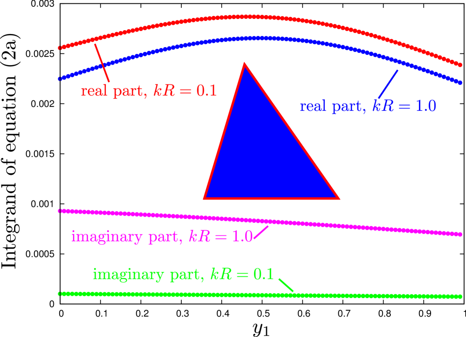
Figure 4: TDM integrand in the common-triangle case for a once-integrable kernel. Plotted is the integrand of equation (2a) with polynomial $P=P^{\hbox{\tiny{EFIE1}}}$ and kernel $K=K^{\hbox{\tiny{EFIE}}}$ (Section V) for two different values of the wavenumber $k$. The triangle lies in the $xy$ plane with vertices at the points $(x,y)=(0,0),(0.1,0),(0.03,0.1).$ The integrand is smooth and amenable to low-order numerical quadrature.

Figure 4 plots the integrand of equation (2a) for the choice of polynomial $P^{\hbox{\scriptsize{EFIE1}}}(\mathbf{x},\mathbf{x}^{\prime})\propto(\mathbf{x}-\mathbf{Q})\cdot(\mathbf{x}-\mathbf{Q}^{\prime})$ and kernel $K^{\hbox{\scriptsize{EFIE}}}(r)=\frac{e^{ikr}}{4\pi r}$, a combination which arises in the EFIE formulation with RWG functions (Section V). The triangle (inset) lies in the $xy$ plane with vertices at the points $(x,y)=\{(0,0),(0.1,0),(0.03,0.1)\}$ with RWG source/sink vertices $\mathbf{Q}=\mathbf{Q}^{\prime}=(0,0).$ The wavenumber parameter $k$ in the Helmholtz kernel is chosen such that $kR=0.1$ or $kR=1.0$, where $R$ is the radius of the triangle (the maximal distance from centroid to any vertex). Whereas the integrand of the original integral (1) exhibits both singularities and sinusoidal oscillations over its 4-dimensional domain, the integrand of the TDM-reduced integral (2a) is nonsingular and slowly varying and will clearly succumb readily to numerical quadrature; indeed, for both values of $k$ a simple 17-point Clenshaw-Curtis quadrature scheme [28] already suffices to evaluate the integrals to better than 11-digit accuracy. Note that, although the sinusoidal factor in the integrand of the original integral (1) exhibits 10$\times$ more rapid variation for $kR=1.0$ than for $kR=0.1$, the TDM reduction to the 1D integrand smooths this behavior to such an extent that the two cases are nearly indistinguishable in (4).

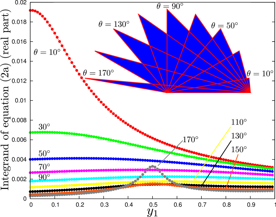
Figure 5: The real part of the integrand of equation (2a) for the case $=P^{\hbox{\tiny{EFIE1}}}$ and kernel $K=K^{\hbox{\tiny{EFIE}}}$ for a triangle in the $xy$ plane with vertices at $(x,y)=(0,0),(L,0),(L\sin\theta,L\cos\theta)$ for $L=0.1$ and 8 distinct values of $\theta$. In each case the wavenumber is $k=0.1/R$ with $R$ the triangle radius.

How are these results modified for triangles of less-regular shapes? Figure 5 plots the real part of the integral of equation (2a), again for the choices $\{P,K\}=\{P^{\hbox{\scriptsize{EFIE1}}},K^{\hbox{\scriptsize{EFIE}}}\},$ for a triangle in the $xy$ plane with vertices $(x,y)=(0,0),(L,0),(L\sin\theta,L\cos\theta)$ with $L=0.1$ and 8 distinct values of $\theta$.

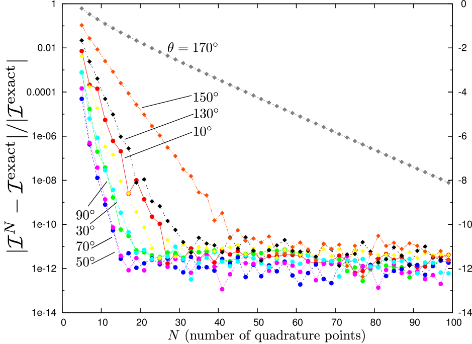
Figure 6: TDM convergence in the common-triangle case for a once-integrable kernel. Plotted is the error vs. number of Clenshaw-Curtis quadrature points incurred by numerical integration of the integrands plotted in Figure 5. ($\mathcal{I}^{N}$ is the $N-$point Clenshaw-Curtis approximant to the integral.)

The integrand exhibits slightly more rapid variation in the extreme cases $\theta=10^{\circ},170^{\circ},$ but remains sufficiently smooth to succumb readily to low-order quadrature. To quantify this, Figure 6 plots, versus $N$, the relative error incurred by numerical integration of the integrands of Figure 5 using $N$-point Clenshaw-Curtis quadrature. (The relative error is defined as $|\mathcal{I}^{N}-\mathcal{I}^{\hbox{\scriptsize{exact}}}|/|\mathcal{I}^{\hbox{\scriptsize{exact}}}|$ where $\mathcal{I}^{N}$ and $\mathcal{I}^{\hbox{\scriptsize{exact}}}$ are the $N$-point Clenshaw-Curtis quadrature approximations to the integral and the “exact” integral as evaluated by high-order Clenshaw-Curtis quadrature (with $N>100$ integrand samples per dimension). For almost all cases we obtain approximately $12$-digit accuracy with just 20 to 30 quadrature points, with only the most extreme-aspect-ratio triangles exhibiting slightly slower convergence. [Note that the $x$-axis quantity $N$ in Figure 6, as well as in Figures 8, 10, and 11, represents the total number of integrand samples required to evaluate the full four-dimensional integral (1), not any lower-dimensional portion of this integral (such as might be the case for other integration schemes that—unlike the method of this paper—divide the original integral into inner and outer “source” and “target” integrals which are handled separately). ]

It is instructive to compare Figures 5 and 6 to Figure 1 of Ref. 4, which applied Duffy-transformation techniques to the two-dimensional integral of $1/r$ over a single triangle (in contrast to the four-dimensional integrals over triangle pairs considered in this work). With the triangle assuming various distorted shapes similar to those in the inset of Figure (5), Ref. 4 observed a dramatic slowing of the convergence of numerical quadrature as the triangle aspect ratio worsened, presumably because the integrand exhibits increasingly rapid variations. In contrast, Figures 5 and 6 indicate that no such catastrophic degradation in integrand smoothness occurs in the four-dimensional case, perhaps because the analytical integrations effected by the TDM reduction from (1) to (2a) smooth the bad integrand behavior that degrades convergence in the two-dimensional case. (Techniques for improving the convergence of two-dimensional integrals over triangles with extreme aspect ratios were discussed in Ref. 29.)

VI-B Common-edge examples

As an example of a common-edge case, Figure 7 plots the two-dimensional integrand of equation (2b) for the choice of polynomial $P^{\hbox{\scriptsize{MFIE}}}=[(\mathbf{x}-\mathbf{Q})\cdot(\mathbf{x}^{\prime}-\mathbf{Q}^{\prime})]\cdot(\mathbf{x}-\mathbf{x}^{\prime})$ and kernel $K^{\hbox{\scriptsize{MFIE}}}(r)=(ikr-1)\frac{e^{ikr}}{4\pi r^{3}}$, a combination which arises in the MFIE formulation with RWG functions (Section V). The triangle pair (inset) is the right-angle pair $\mathcal{T}=\{(0,0,0),(L,0,0),(0,L,0)\}$ and $\mathcal{T}^{\prime}=\{(0,0,0),(L,0,0),(L/2,0,-L)\}$ with $L=0.1.$ The RWG source/sink vertices are indicated by black dots in the inset. The $k$ parameter in the Helmholtz kernel is chosen such that $kR=0.628$ where $R$ is the maximum panel radius. The integrand is smooth and is amenable to straightforward two-dimensional cubature. To quantify this, Figure 8 plots the error vs. number of cubature points incurred by numerical integration of the integrand plotted in Figure 9. The cubature scheme is simply nested two-dimensional Clenshaw-Curtis cubature, with the same number of quadrature points per dimension. Although the added dimension of integration inevitably necessitates the use of more integration points than were needed in the 1D cases examined above, nonetheless we achieve 12-digit accuracy with roughly 500 cubature points.

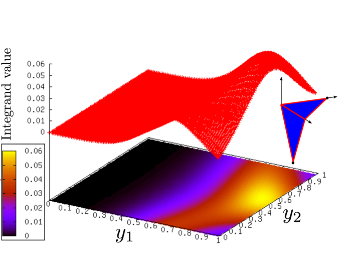
Figure 7: TDM integrand for a common-edge case with a once-integrable kernel. Plotted is the integrand of equation (2b) with polynomial $P=P^{\hbox{\scriptsize{MFIE}}}$ and kernel $K=K^{\hbox{\scriptsize{MFIE}}}$ for a right-angle common-edge panel pair (inset).

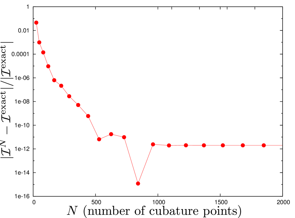
Figure 8: TDM convergence for a common-edge case with a once-integrable kernel. Plotted is the error vs. the total number of cubature points incurred by numerical integration of the integrand plotted in Figure 7. The cubature scheme is simple two-dimensional nested Clenshaw-Curtis quadrature with equal numbers of quadrature points in each dimension.

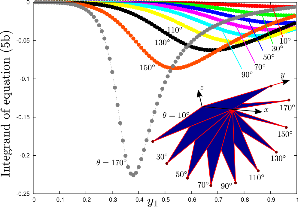
Figure 9: TDM integrand in a common-edge case with a twice-integrable kernel. Plotted is the integrand of equation (5b) with polynomial $P=P^{\hbox{\tiny{MFIE}}}$ and kernel $K(r)=\frac{1}{4\pi r^{3}}$ for common-edge panel pairs ranging from nearly coplanar ($\theta=10^{\circ}$) to right-angle ($\theta=90^{\circ}$) to nearly coincident ($\theta=170^{\circ}$). In all cases the integrand is well-behaved and amenable to low-order numerical quadrature (see Figure 10).

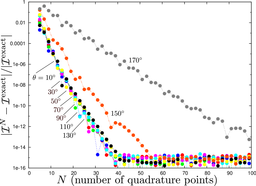
Figure 10: TDM convergence in a common-edge case for a twice-integrable kernel. Plotted is the error vs. number of quadrature points incurred by numerical integration of the integrands plotted in Figure 9. The cubature scheme is Clenshaw-Curtis quadrature. The convergence rate is essentially independent of the angle $\theta$ between the normals to the panels except for the near-singular case $\theta=170^{\circ}.$

The kernel $K^{\hbox{\scriptsize{MFIE}}}(r)$ approaches $-1/(4\pi r^{3})$ for small $r$. (As noted above, pairing with $P^{\hbox{\scriptsize{MFIE}}}$ reduces the singularity of the overall integrand due to the vanishing of $P^{\hbox{\scriptsize{MFIE}}}$ at $r=0$.) If we consider the integral of just this most singular contribution—that is, if in (1) we retain the polynomial $P=P^{\hbox{\scriptsize{MFIE}}}$ but now replace the kernel $K^{\hbox{\scriptsize{MFIE}}}(r)$ with $K(r)=1/(4\pi r^{3})$—then we have a twice-integrable kernel and the Taylor-Duffy reduction yields a one-dimensional integral, equation (5b), instead of the two-dimensional integrand (2b) plotted in (7). Figure 9 plots the 1-dimensional integrand obtained in this way for several common-edge panel pairs obtained by taking the unshared vertex of $\mathcal{T}^{\prime}$ to be the point $(L/2,-L\cos\theta,-L\sin\theta)$ with $\theta$ ranging from $\theta=10^{\circ}$ to $170^{\circ}$. (The inset of Figure 7 corresponds to $\theta=90^{\circ}.$) For all values of $\theta$ the integrand is smooth and readily amenable to numerical quadrature. Figure 10 plots the convergence vs. number of quadrature points for numerical integration by Clenshaw-Curtis quadrature of the integrands plotted in Figure 9. The convergence rate is essentially independent of $\theta$ throughout the entire range $\theta\in[0,130^{\circ}].$

VI-C Common-vertex example

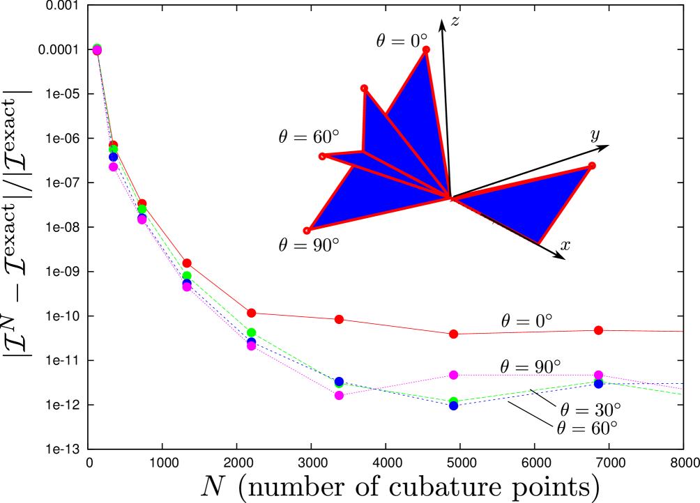
Figure 11: TDM convergence in a common-vertex case for a once-integrable kernel. Plotted is the error vs. number of cubature points incurred by numerical integration of Equation 2(c) for the common-vertex triangle pairs shown in the inset (see text) and polynomial/kernel pair $\{P,K\}$=$\{P^{\hbox{\tiny{EFIE1}}},K^{\hbox{\tiny{EFIE}}}\}$. The convergence rate is essentially independent of the angle $\theta$.

As an example of a common-vertex case, Figure 11 plots the convergence of equation (2c) for $\{P,K\}$=$\{P^{\hbox{\scriptsize{EFIE1}}},K^{\hbox{\scriptsize{EFIE}}}\}$, the same pair considered for the common-triangle example above. The triangle pair (inset) is $\mathcal{T}=\{(0,0,0),(L,0,0),(L^{\prime},L,0)\}$ and $\mathcal{T}^{\prime}=\{(0,0,0),(-L,0,0),(-L^{\prime}\sin\theta,L^{\prime}\cos\theta)\}$ with $\{L,L^{\prime}\}=\{0.1,0.02\}$ and various values of $\theta$. The $k$ parameter in the Helmholtz kernel is chosen such that $kR=0.628$ where $R$ is the maximum panel radius. RWG source/sink vertices are indicated by dots in the inset. The figure plots the error vs. number of cubature points incurred by numerical integration of the integrand plotted in Figure 9. The cubature scheme is simply nested three-dimensional Clenshaw-Curtis cubature, with the same number of quadrature points per dimension. This is probably not the most efficient cubature scheme for a three-dimensional integral, but the figure demonstrates that the error decreases steadily and rapidly with the number of cubature points. The convergence rate is essentially independent of $\theta$.

VII Application to Full-Wave BEM Solvers: Evaluation and Caching of Series-Expansion Terms

We now take up the question of how the generalized TDM may be most effectively deployed in practical implementations of full-wave BEM solvers using RWG basis functions. To assemble the BEM matrix for, say, the PMCHWT formulation at a single frequency for a geometry discretized into $N$ triangular surface panels, we must in general compute $\approx\,12N$ singular integrals of the form (1) with roughly $\{2N,4N,6N\}$ instances of the common-{triangle, edge, vertex} cases. [For each panel pair we must compute integrals involving two separate kernels ($K^{\hbox{\scriptsize{EFIE}}}$ and $K^{\hbox{\scriptsize{MFIE}}}$), and neither of these kernels is twice-integrable except in the short-wavelength limit.]

A first possibility is simply to evaluate all singular integrals using the basic TDM scheme outlined in Section II—that is, for an integral of the form (1) with polynomial $P(\mathbf{x},\mathbf{x}^{\prime})$ and kernel $K(r)$ we write simply

$$\mathcal{I}=\underbrace{\iint P(\mathbf{x},\mathbf{x}^{\prime})K(r)d\mathbf{x}^{\prime}d\mathbf{x}.}_{\text{evaluate by TDM}}$$ (17)

This method already suffices to evaluate all singular integrals and would consitute an adequate solution for a medium-performance solver appropriate for small-to-midsized problems. However, although the unadorned TDM successfully neutralizes singularities to yield integrals amenable to simple numerical cubature, we must still evaluate those 1D-, 2D-, and 3D cubatures, and this task, even given the non-singular integrands furnished by the TDM, remains too time-consuming for the online stage of a high-performance BEM code for large-scale probems.

Instead, we propose here to accelerate the bare TDM using singularity-subtraction (SS) techniques [4, 5, 6]. Subtracting from $K(r)$ the first $M$ terms in its small-$r$ series expansion, we write

$$K(r)=\sum_{m=0}^{M-1}C_{m}r^{m-L}+K^{\hbox{\scriptsize{NS}}}(r)$$ (18)

where $K^{\hbox{\scriptsize{NS}}}$ is nonsingular. Here $L$ is the most singular power of $1/r$ in the small-$r$ expansion of $K(r)$; for $\{K^{\hbox{\scriptsize{EFIE}}},K^{\hbox{\scriptsize{MFIE}}}\}$ we have $L=\{1,3\}$. (As noted below, we typically choose $M>L$, i.e. we subtract more than the minimal number of terms required to desingularize the kernel.) Equation (17) becomes

$$\mathcal{I} =\sum_{m=0}^{M-1}C_{m}\underbrace{\iint P(\mathbf{x},\mathbf{x}^{\prime})r^{m-L}d\mathbf{x}^{\prime}d\mathbf{x}}_{\text{evaluate by TDM}}$$ (19)

$$\qquad+\underbrace{\iint P(\mathbf{x},\mathbf{x}^{\prime})K^{\hbox{\scriptsize{NS}}}(r)d\mathbf{x}^{\prime}d\mathbf{x}}_{\text{evaluate by cubature}}$$

The first set of terms on the RHS of (19) involve integrals of the form (1) with kernels $r^{p}$, which we evaluate using the generalized TDM proposed in this paper. The last term is a nonsingular integral which we evaluate using simple low-order numerical cubature. Such a hybrid TDM-SS approach has several advantages. (a) The integrals involving the $r^{p}$ kernel are independent of frequency and material properties, even if $K(r)$ depends on these quantities through the wavenumber $k=\sqrt{\epsilon\mu}\cdot\omega$. [The $k$ dependence of the first set of terms in (19) is contained entirely in the constants $\{C_{m}\}$, which enter only as multiplicative prefactors outside the integral sign.] This means that we need only compute these integrals once for a given geometry, after which they may be stored and reused many times for computations at other frequencies or for scattering geometries involving the same shapes but different material properties. (The caching and reuse of frequency-independent contributions to BEM integrals has been proposed before [4].) (b) The $r^{p}$ kernels in the first set of integrals are twice-integrable. This means that the improved Taylor-Duffy scheme discussed in Section III is available, significantly accelerating the computation; for the common-triangle case these integrals maybe evaluated in closed analytical form. (c) The $M$ integrals in the first set all involve the same $P$ polynomial. This means that the computational overhead required to evaluate TDM integrals involving this polynomial need only be done once and may then be reused for all $M$ integrals. Indeed, all of the integrals on the first line of (19) may be evaluated simultaneously as the integral of an $M$-dimensional vector-valued integrand; in practice this means that the cost of evaluating all $M$ integrals is nearly independent of $M$. (d) Because $K^{\hbox{\scriptsize{NS}}}$ has been relieved of its most rapidly varying contributions, it may be integrated with good accuracy by a simple low-order cubature scheme. {We evaluate the 4-dimensional integral in the last term of (19) using a 36-point cubature rule [30].}

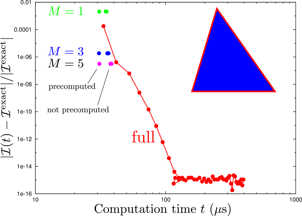
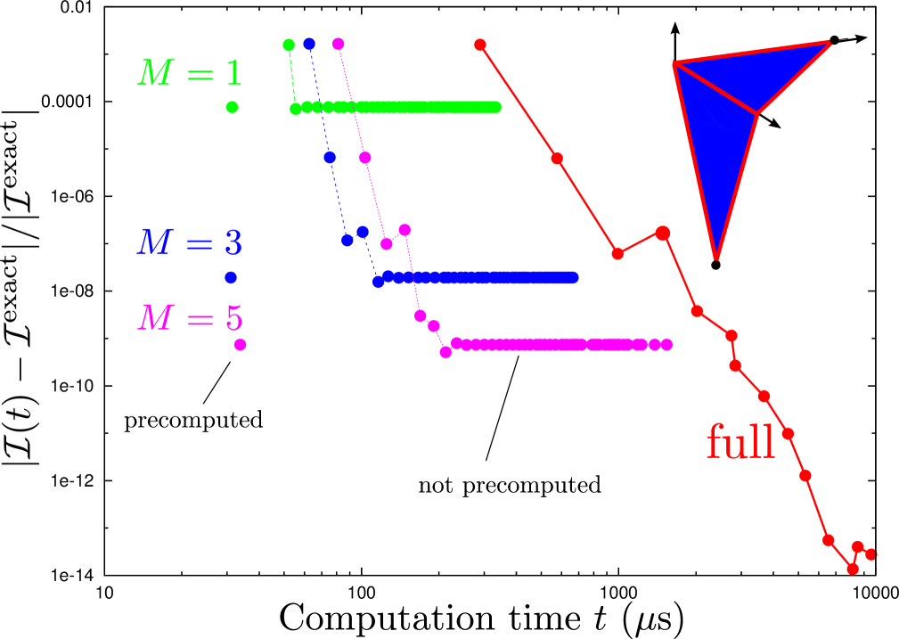
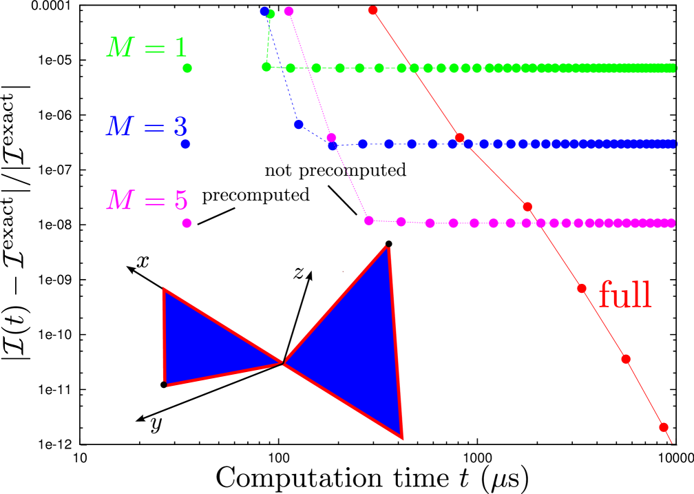
Figure 12: Accuracy vs. computation time for approaches to evaluating singular integrals. Top: Common-triangle case with the triangle of Figure 4. Center: Common-edge case with the triangle of Figure 7. Bottom: Common-vertex case with the $\theta=30^{\circ}$ triangle of Figure 11. In each case the integral considered is (1) with $\{P,K\}=\{P^{\hbox{\tiny{EFIE1}}},K^{\hbox{\tiny{EFIE}}}\}$ (Section V). The wavenumber $k$ is chosen such that $kR=0.628$ where $R$ is the maximum panel radius, i.e. the linear size of the panel is approximately 1/10 the wavelength. Curves marked “full” correspond to equation (17), i.e. numerical cubature of the 1, 2, or 3-dimensional integral in equation (2). Curves marked $M=\{1,3,5\}$ correspond to the singularity-subtraction scheme of equation (19); the singular integrals are evaluated by numerical cubature of the 0, 1, or 2-dimensional integral in equation (5), while the remaining (non-singular) integral is evaluated using a 36-point four-dimensional numerical cubature scheme. All TDM integrals are evaluated using Clenshaw-Curtis quadrature (nested for 2- and 3-dimensional integrals).

Figure 12 compares accuracy vs. computation time for the methods of equation (17) and equation (19) with $M=\{1,3,5\}$ subtracted terms. The {top, center, bottom} plots are for the {CT, CE, CV} cases using the triangle pairs of Figures {4, 7, 11} (we choose the $\theta=30^{\circ}$ triangle pair for the CV case). The integral computed is (1) with $\{P,K\}=\{P^{\hbox{\scriptsize{EFIE1}}},K^{\hbox{\scriptsize{EFIE}}}\}$. The wavenumber $k$ is chosen such that $kR=0.628$ where $R$ is the maximum panel radius, so that the linear size of the panels is approximately 1/10 the wavelength.

The curves marked “full” in each plot correspond to equation (17), i.e. full evaluation by numerical cubature of the (1,2,3)-dimensional integral of equation (2). The $M=\{1,3,5\}$ data correspond to equation (19). For each $M$ value, the data point furthest to the left is for the case in which we precompute the contributions of the singular integrals, so that the only computation time is the evaluation of the fixed-order cubature. The other data points for each $M$ value include the time incurred for numerical cubature of equation (5) for the subtracted (singular) terms at varying degrees of accuracy. Beyond a certain threshold computation time the integrals have converged to accurate values, whereupon further computation time does not improve the accuracy with which we compute the overall integral (because we use a fixed-order cubature for the nonsingular contribution). Of course, one could increase the cubature order for the fixed-order contribution at the expense of shifting all $M=\{1,3,5\}$ data points to the right.

In the common-triangle case, the integrals of the singular terms may be done in closed form [equation (5a)], so the data points marked “not precomputed” all correspond to roughly the same computation time. In the other cases, the “not precomputed” data points for various values of the computation time correspond to evaluation of the integrals (5b) or (5c) via numerical cubature with varying numbers of cubature points.

Absolute timing statistics are of course heavily hardware- and implementation-dependent (in this case they were obtained on a standard desktop workstation), but the picture of relative timing that emerges from Figure 12 is essentially hardware-independent. For a given accuracy, the singularity-subtracted scheme (19) is typically an order of magnitude faster than the full scheme (17), and this is true even if we include the time required to compute the integrals of the frequency-independent subtracted terms. If we precompute those integrals, the singularity-subtraction scheme is several orders of magnitude faster than the full scheme. For example, to achieve 8-digit accuracy in the common-vertex case takes over 2 ms for the full scheme but just 30 $\mu$s for the precomputed $M=5$ singularity-subtraction scheme.

The speedup effected by singularity subtraction is less pronounced in the common-triangle case. This is because the full TDM integral (17) is only 1-dimensional in that case and thus already quite efficient to evaluate.

VIII Helmholtz-Kernel Integrals in the Short-Wavelength Limit

The kernels $K^{\hbox{\scriptsize{EFIE}}}(r)=\frac{e^{ikr}}{4\pi r}$ and $K^{\hbox{\scriptsize{MFIE}}}(r)=(ikr-1)\frac{e^{ikr}}{4\pi r^{3}}$ become twice-integrable in the limit $\text{Im }k\to\infty.$ More specifically, as shown in Appendix B, the first integral [equation (3)] of these kernels takes the form $Q_{1}(r)+e^{ikX(r)}Q_{2}(r)$, where $Q_{1},Q_{2}$ are Laurent polynomials in $r$ and $X$ is a nonvanishing quantity bounded below by the linear size of the triangles. When $\text{Im }k$ is large, the exponential factor makes the second term negligible, and we are left with just $Q_{1}(r)$—which, as a sum of integer powers of $r$—is twice-integrable. This means that the TDM-reduced version of integral (1) involves one fewer dimension of integration than in the usual case, i.e. we have equations (5) instead of equations (2). In particular, for the common-triangle case the full integral may be evaluated in closed form [equation (5a)].

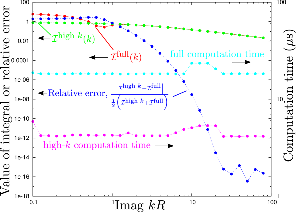
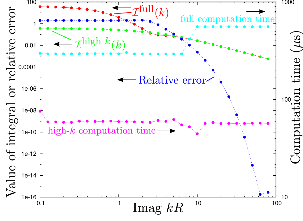
Figure 13: Accuracy and computation time for evaluation of integral (1) for $\{P,K\}=\{1,\frac{e^{ikr}}{4\pi r}\}$ via equations (2) and (5). Upper plot: Common-triangle case for the triangle of Figure 4. Lower plot: Common-edge case for the triangle pair of Figure 7. The $x$-axis measures the imaginary part of the wavenumber $k$ in the Helmholtz kernel. The real part of $k$ is fixed at Re $kR=0.628$ where $R$ is the maximum panel radius. In each case, the red curve is the value of the $\{1,2\}$-dimensional integral computed using the “full” equation (2), while the green curve is the value of the $\{0,1\}$-dimensional integral computed using the “high-$k$” approximation to the integral involving equation (5). The blue curve is the relative error between the two calculations (their difference divided by their average). The cyan and magenta curves, respectively plot the (wall-clock) time required to evaluate the integrals via the “full” and “high-$k$” schemes.

Figure 13 plots, for the common-triangle case of Figure 4 (upper plot) and the common-edge case of Figure 7 (lower plot), values and computation times for the integral $\iint\frac{e^{ikr}}{4\pi r}\,d^{4}r$—that is, equation (1) for the choices $\{P,K\}=\{1,K^{\hbox{\scriptsize{EFIE}}}\}$—as evaluated using the “full” scheme of equation (2) (red curves) and using the “high-$k$ approximation” of equation (5) (green curves), with the exponentially-decaying term in the first integral of the kernel neglected to yield a twice-integrable kernel. The blue curves are the relative errors between the two calculations. The cyan and magenta curves respectively plot the (wall-clock) time required to compute the integrals using the full and high-$k$ methods. The high-$k$ calculation is approximately one order of magnitude more rapid than the full calculation and yields results in good agreement with the full calculation for values of Imag $kR$ greater than 10 or so.

IX Conclusions

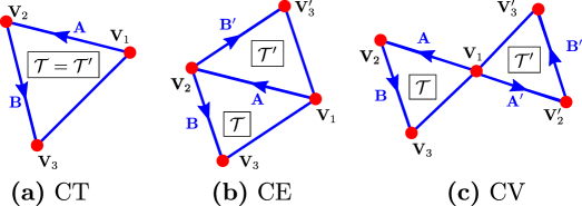
Figure 14: Labeling of triangle vertices and edges. (a) The common-triangle case. (b) The common-edge case. (c) The common-vertex case.

The generalized Taylor-Duffy method we have presented allows efficient evaluation of a broad family of singular and non-singular integrals over triangle-pair domains. The generality of the method allows a single implementation ($\sim$1,500 lines of C++ code) to handle all singular integrals arising in several different BEM formulations, including electrostatics with triangle-pulse basis functions and full-wave electromagnetism with RWG basis functions in the EFIE, MFIE, PMCHWT, and N-Müller formulations. In particular, for N-Müller integrals the method presented here offers an alternative to the line-integral scheme discussed in Ref. 4. In addition to deriving the method and discussing practical implementation details, we presented several computational examples to illustrate its efficacy.

Although the examples we considered here involved low-order basis functions (constant or linear variation over triangles), it would be straightforward to extend the method to higher-order basis functions. Indeed, switching to basis functions of quadratic or higher order would amount simply to choosing different $P$ polynomials in (1); the computer-algebra methods mentioned in Section IV could then be used to identify the corresponding $\mathcal{P}$ polynomials in equations (2) and (5). A less straightforward but potentially fruitful challenge would be to extend the method to the case of curved triangles, in which case the integrand of (1) may contain non-polynomial factors [31].

Although—as noted in the Introduction—the problem of evaluating singular BEM integrals has been studied for decades with dozens of algorithms published, the problem of choosing which of the myriad available schemes to use in a practical BEM solver must surely remain bewildering to implementors. A comprehensive comparative survey of available methods—including considerations such as numerical accuracy vs. computation time, the reuse of previous computations to accelerate calculations at new frequencies, the availability of open-source code implementations, and the complexity and length of codes versus their extendability and flexibility (i.e. the range of possible integrands they can handle)—would be an invaluable contribution to the literature.

A complete implementation of the method described in this paper is incorporated into scuff-em, a free, open-source software implementation of the boundary-element method [1].

Appendix A Expressions for subregion-dependent functions

The TDM formulas (2) refer to functions $X_{d}$ and $\mathcal{P}_{dn}$ indexed by the subregion $d$ of the original 4-dimensional integration domain. In this Appendix we give detailed expressions for these quantities. In what follows, the geometric parameters $\mathbf{A},\mathbf{B},\mathbf{A}^{\prime},\mathbf{B}^{\prime},\mathbf{V}_{i}$ refer to Figure 14, and the functions $\mathbf{x}(\xi_{1},\xi_{2})$ and $\mathbf{x}^{\prime}(\eta_{1},\eta_{2})$ map the standard triangle into $\mathcal{T},\mathcal{T}^{\prime}$ according to

$$\mathbf{x}(\xi_{1},\xi_{2})=\mathbf{V}_{1}+\xi_{1}\mathbf{A}+\mathbf{\xi}_{2}\mathbf{B},\quad\mathbf{x}^{\prime}(\eta_{1},\eta_{2})=\mathbf{V}_{1}+\eta_{1}\mathbf{A}^{\prime}+\eta_{2}\mathbf{B}^{\prime}.$$ (20)

with ranges $0\leq\xi_{1},\eta_{1}\leq 1$, $0\leq\xi_{2}\leq\xi_{1}$, $0\leq\eta_{2}\leq\eta_{1}.$

Common Triangle

$u$ functions

First define ancillary functions $u_{1}$ and $u_{2}$ depending on $y_{1}$:

$$\begin{array}[]{|c|c|c|}\hline\cr d&u_{1d}(y_{1})&u_{2d}(y_{1})\\ \hline\cr 1&1&y_{1}\\ \hline\cr 2&y_{1}&(y_{1}-1)\\ \hline\cr 3&y_{1}&1\\ \hline\cr\end{array}$$ (21)

Reduced distance function

The function $X^{\hbox{\tiny{CT}}}_{d}(y_{1})$ that enters formulas (2a) and (5a) is

$$\!\!X_{d}^{\hbox{\tiny{CT}}}(y_{1})$$

$$=\sqrt{|\mathbf{A}|^{2}u_{1d}^{2}(y_{1})+|\mathbf{B}|^{2}u_{2d}^{2}(y_{1})+2\mathbf{A}\cdot\mathbf{B}u_{1d}(y_{1})u_{2d}(y_{1})}.$$

$\mathcal{P}$ polynomials

First define polynomials obtained as definite integrals over the original $P$ polynomial in (1):

$$H_{d}(u_{1},u_{2})\equiv 4AA^{\prime}\int_{\xi_{1d}^{\hbox{\scriptsize{lower}}}}^{\xi_{1d}^{\hbox{\scriptsize{upper}}}}d\xi_{1}\int_{\xi_{2d}^{\hbox{\scriptsize{lower}}}}^{\xi_{2d}^{\hbox{\scriptsize{upper}}}}d\xi_{2}\,\bigg{\{}$$

$$P\Big{(}\mathbf{x}(\xi_{1},\xi_{2}),\mathbf{x}^{\prime}(u_{1}+\xi_{1},u_{2}+\xi_{2})\Big{)}$$

$$\,\,+P\Big{(}\mathbf{x}(u_{1}+\xi_{1},u_{2}+\xi_{2}),\mathbf{x}^{\prime}(\xi_{1},\xi_{2})\Big{)}\bigg{\}}$$ (22)

where $\mathbf{x}(\xi_{1},\xi_{2})$ and $\mathbf{x}^{\prime}(\eta_{1},\eta_{2})$ are as in (20) and where the limits of the $\xi_{1},\xi_{2}$ integrals are as follows:

$$\begin{array}[]{|c|c|c|c|c|}\hline\cr d&\xi_{1d}^{\hbox{\tiny{lower}}}&\xi_{1d}^{\hbox{\tiny{upper}}}&\xi_{2d}^{\hbox{\tiny{lower}}}&\xi_{2d}^{\hbox{\tiny{upper}}}\\ \hline\cr 1&0&1-u_{1}&0&\xi_{1}\\ \hline\cr 2&-u_{2}&1-u_{1}&-u_{2}&\xi_{1}\\ \hline\cr 3&u_{2}-u_{1}&1-u_{1}&0&\xi_{1}-(u_{2}-u_{1})\\ \hline\cr\end{array}$$ (23)

Now evaluate $H_{d}$ at $w,y_{1}$ dependent arguments and expand the result as a polynomial in $w$ to obtain the $\mathcal{P}_{dn}^{\hbox{\tiny{CT}}}$ functions:

$$H_{d}\Big{(}wu_{1d}(y_{1}),wu_{2d}(y_{1})\Big{)}\equiv\sum_{n}w^{n}\mathcal{P}_{dn}^{\hbox{\tiny{CT}}}(y_{1}).$$ (24)

Common Edge

$u,\xi$ functions

First define ancillary functions $u_{1},u_{2},\xi_{2}$ depending on $y_{1}$ and $y_{2}$:

$$\begin{array}[]{|c|c|c|c|}\hline\cr d&u_{1d}(y_{1},y_{2})&u_{2d}(y_{1},y_{2})&\xi_{2d}(y_{1},y_{2})\\ \hline\cr 1&-y_{1}&-y_{1}y_{2}&1-y_{1}+y_{1}y_{2}\\ \hline\cr 2&y_{1}&y_{1}y_{2}&1-y_{1}\\ \hline\cr 3&-y_{1}y_{2}&y_{1}(1-y_{2})&1-y_{1}\\ \hline\cr 4&y_{1}y_{2}&-y_{1}(1-y_{2})&1-y_{1}y_{2}\\ \hline\cr 5&-y_{1}y_{2}&-y_{1}&1\\ \hline\cr 6&y_{1}y_{2}&y_{1}&1-y_{1}\\ \hline\cr\end{array}$$ (25)

Reduced distance function

The function $X^{\hbox{\tiny{CE}}}_{d}(y_{1},y_{2})$ that enters formulas (2b) and (5b) is

$$X_{d}^{\hbox{\tiny{CE}}}(y_{1},y_{2})=\bigg{[}|\mathbf{A}|^{2}u_{1d}^{2}+|\mathbf{B}^{\prime}|^{2}u_{2d}^{2}+|\mathbf{L}|^{2}\xi_{2d}^{2}$$

$$\,\,\,+2\mathbf{A}\cdot\mathbf{B}^{\prime}u_{1d}u_{2d}+2\mathbf{A}\cdot\mathbf{L}u_{1d}\xi_{2d}+2\mathbf{B}^{\prime}\cdot\mathbf{L}u_{2d}\xi_{2d}\bigg{]}^{1/2}$$

where $u_{1d},u_{2d},\xi_{2d}$ are functions of $y_{1}$ and $y_{2}$ as in (25), and where $\mathbf{L}\equiv\mathbf{B}^{\prime}-\mathbf{B}$.

$\mathcal{P}$ polynomials

First define polynomials obtained as definite integrals over the original $P$ polynomial in (1):

$$\!\!H_{d}(u_{1},u_{2},\xi_{2})$$

$$\equiv 4AA^{\prime}\int_{\xi_{1d}^{\hbox{\scriptsize{lower}}}}^{\xi_{1d}^{\hbox{\scriptsize{upper}}}}d\xi_{1}\bigg{\{}P\Big{(}\mathbf{x}(\xi_{1},\xi_{2}),\mathbf{x}^{\prime}(u_{1}+\xi_{1},u_{2}+\xi_{2})\Big{)}\bigg{\}}$$

where $\mathbf{x}(\xi_{1},\xi_{2})$ and $\mathbf{x}^{\prime}(\eta_{1},\eta_{2})$ are as in (20) and where the limits of the $\xi_{1}$ integral are as follows:

$$\begin{array}[]{|c|c|c|c|c|}\hline\cr d&\xi_{1d}^{\hbox{\tiny{lower}}}&\xi_{1d}^{\hbox{\tiny{upper}}}\\ \hline\cr 1&\xi_{2}+(u_{2}-u_{1})&1\\ \hline\cr 2&\xi_{2}&1-u_{1}\\ \hline\cr 3&\xi_{2}+(u_{2}-u_{1})&1\\ \hline\cr 4&\xi_{2}&1-u_{1}\\ \hline\cr 5&\xi_{2}&1\\ \hline\cr 6&\xi_{2}+(u_{2}-u_{1})&1-u_{1}\\ \hline\cr\end{array}.$$

Now evaluate $H_{d}$ at $w,y_{1},y_{2}$-dependent arguments and expand the result as a polynomial in $w$ to obtain the $\mathcal{P}_{dn}^{\hbox{\tiny{CE}}}$ functions:

$$H_{d}\Big{(}wu_{1d}(y_{1},y_{2}),wu_{2d}(y_{1},y_{2}),w\xi_{2}(y_{1},y_{2})\Big{)}$$

$$\quad\equiv\sum_{n}w^{n}\mathcal{P}_{dn}^{\hbox{\tiny{CE}}}(y_{1},y_{2}).$$ (26)

Common Vertex

$\xi,\eta$ functions

First define ancillary functions $\xi_{1},\xi_{2},\eta_{1},\eta_{2}$ depending on $y_{1},y_{2},y_{3}$:

$$\begin{array}[]{|c|c|c|c|c|}\hline\cr d&\xi_{1d}(\mathbf{y})&\xi_{2d}(\mathbf{y})&\eta_{1d}(\mathbf{y})&\eta_{2d}(\mathbf{y})\\ \hline\cr 1&1&y_{1}&y_{2}&y_{2}y_{3}\\ \hline\cr 2&y_{2}&y_{2}y_{3}&1&y_{1}\\ \hline\cr\end{array}$$ (27)

Reduced distance function

The function $X^{\hbox{\tiny{CV}}}_{d}(y_{1},y_{2},y_{3})$ that enters formulas (2c) and (5c) is

$$X_{d}^{\hbox{\tiny{CV}}}(y_{1},y_{2},y_{3})$$

$$=\bigg{[} |\mathbf{A}|^{2}\xi_{1d}^{2}+|\mathbf{B}|^{2}\xi_{2d}^{2}+|\mathbf{A}^{\prime}|^{2}\eta_{1d}^{2}+|\mathbf{B}^{\prime}|^{2}\eta_{1d}^{2}$$

$$+2\big{(}\mathbf{A}\cdot\mathbf{B}\big{)}\xi_{1d}\xi_{2d}-2\big{(}\mathbf{A}\cdot\mathbf{A}^{\prime}\big{)}\xi_{1d}\eta_{1d}$$

$$-2\big{(}\mathbf{A}\cdot\mathbf{B}^{\prime}\big{)}\xi_{1d}\eta_{2d}-2\big{(}\mathbf{B}\cdot\mathbf{A}^{\prime}\big{)}\xi_{2d}\eta_{1d}$$

$$-2\big{(}\mathbf{B}\cdot\mathbf{B}^{\prime}\big{)}\xi_{2d}\eta_{2d}+2\big{(}\mathbf{A}^{\prime}\cdot\mathbf{B}^{\prime}\big{)}\eta_{1d}\eta_{2d}\bigg{]}^{1/2}$$

where $\xi$ and $\eta$ are functions of $y_{1},y_{2},$ and $y_{3}$ as in (27).

$\mathcal{P}$ polynomials

In contrast to the common-triangle and common-edge cases, in the common-vertex case there is no integration over the original $P$ polynomial; instead, we simply evaluate the original $P$ polynomial at $w$- and $\mathbf{y}$-dependent arguments, expand the result as a power series in $w$, and identify the coefficients of this power series as the $\mathcal{P}(\mathbf{y})$ polynomials:

$$P\Big{(}w\xi_{1d}(\mathbf{y}),w\xi_{2d}(\mathbf{y}),w\eta_{1d}(\mathbf{y}),w\eta_{2d}(\mathbf{y})\Big{)}\equiv\sum_{n}w^{n}\mathcal{P}_{dn}^{\hbox{\tiny{CV}}}(\mathbf{y}).$$ (28)

The $\alpha$, $\beta$, $\gamma$ Coefficients

For twice-integrable kernels, the master TDM formulas (5) refer to parameters $\alpha$, $\beta$, and $\gamma$ defined for the various cases and the various subregions. These parameters are defined by completing the square under the radical sign in the reduced-distance functions $X_{d}$:

$$X_{d}^{\hbox{\tiny{CT}}}(y_{1}) \equiv\sqrt{\alpha^{\hbox{\tiny{CT}}}_{d}(y_{1}+\beta^{\hbox{\tiny{CT}}}_{d})^{2}+\gamma^{\hbox{\tiny{CT}}}_{d}}$$

$$X_{d}^{\hbox{\tiny{CE}}}(y_{1},y_{2}) \equiv\sqrt{\alpha^{\hbox{\tiny{CE}}}_{d}(y_{2}+\beta^{\hbox{\tiny{CE}}}_{d})^{2}+\gamma^{\hbox{\tiny{CE}}}_{d}}$$

$$X_{d}^{\hbox{\tiny{CV}}}(y_{1},y_{2},y_{3}) \equiv\sqrt{\alpha^{\hbox{\tiny{CV}}}_{d}(y_{3}+\beta^{\hbox{\tiny{CV}}}_{d})^{2}+\gamma^{\hbox{\tiny{CV}}}_{d}}$$

In all cases, the $\{\alpha,\beta,\gamma\}$ coefficients depend on the geometric parameters ($\mathbf{A},\mathbf{B},$ etc.). In the CE case, they depend additionally on the variable $y_{1}$, and in the CV case they depend additionally on the variables $y_{1}$ and $y_{2}$.

Appendix B First and Second Kernel Integrals

In this Appendix we collect expressions for the first and second integrals of various commonly encountered kernel functions.

First Kernel Integrals

In Section II we defined the “first integral” of a kernel function $K(r)$ to be

$$\mathcal{K}_{n}(X)\equiv\int_{0}^{1}w^{n}K(wX)\,dw.$$

First integrals for some commonly encountered kernels are presented in Table I.

$$\begin{array}[]{|c|c|}\hline\cr\ K(r)&\mathcal{K}_{n}(X)\\ \hline\cr r^{p}&\displaystyle{\frac{X^{p}}{1+n+p}}\vphantom{\int_{\int}^{\int}}\\ \hline\cr\displaystyle{\frac{e^{ikr}}{4\pi r}}&\displaystyle{\frac{e^{ikX}}{4\pi nX}\text{ExpRel}(n,-ikX)}\\[5.0pt] \hline\cr\displaystyle{(ikr-1)\frac{e^{ikr}}{4\pi r^{3}}}&\parbox{130.08731pt}{ \@@amsalign&\displaystyle{\frac{e^{ikX}}{4\pi X}\bigg{[}\frac{ik}{(n-1)X}\text{ExpRel}(n-1,-ikX)}\\ &\qquad\qquad\displaystyle{-\frac{1}{(n-2)X^{2}}\text{ExpRel}(n-2,-ikX)\bigg{]}} }\vphantom{\int_{\int}^{\int}}\\ \hline\cr\end{array}$$

TABLE I: First integrals for some relevant kernel functions.

The function ExpRel$(n,z)$ in Table I is the $n$th “relative exponential” function, defined as the usual exponential function with the first $n$ terms of its power-series expansion subtracted and the result normalized to have value 1 at $z=0$:

$$\text{ExpRel}(n,z) \equiv\frac{n!}{z^{n}}\Big{[}e^{z}-1-z-\frac{z^{2}}{2}-\cdots-\frac{z^{n-1}}{(n-1)!}\Big{]}$$ (29a)

$$=1+\frac{z}{(n+1)}+\frac{z^{2}}{(n+1)(n+2)}+\cdots$$ (29b)

For $|z|$ small, the relative exponential function may be computed using the rapidly convergent series expansion (29b), and indeed for computational purposes at small $z$ it is important not to use the defining expression (29a), naïve use of which invites catastrophic loss of numerical precision. For example, at $z=10^{-4}$, each term subtracted from $e^{z}$ in the square brackets in (29a) eliminates 4 digits of precision, so that in standard 64-bit floating-point arithmetic a calculation of $\text{ExpRel}(3,z)$ would be accurate only to approximately 3 digits, while a calculation of $\text{ExpRel}(4,z)$ would yield pure numerical noise.

On the other hand, for values of $z$ with large negative real part—which arise in calculations involving lossy materials at short wavelengths—it is most convenient to evaluate ExpRel in a different way, as discussed below.

Second Kernel Integrals for the $r^{p}$ kernel

In Section III we defined the “second integrals” of a kernel function $K(r)$ to be the following definite integrals involving the first integral:

$$\mathcal{J}_{n}(\alpha,\beta,\gamma) \equiv\int_{0}^{1}\mathcal{K}_{n}\Big{(}\alpha\sqrt{(y+\beta)^{2}+\gamma^{2}}\Big{)}\,dy$$ (30)

$$\mathcal{L}_{n}(\alpha,\beta,\gamma) \equiv\int_{0}^{1}y\,\mathcal{K}_{n}\Big{(}\alpha\sqrt{(y+\beta)^{2}+\gamma^{2}}\Big{)}\,dy.$$ (31)

For the particular kernel function $K(r)=r^{p}$ with (positive or negative) integer power $p$, the second integrals are the following analytically-evaluatable integrals:

$$\mathcal{J}_{n}(\alpha,\beta,\gamma) =\frac{\alpha^{p}}{(1+p+n)}\underbrace{\int_{0}^{1}\Big{[}(y+\beta)^{2}+\gamma^{2}]^{p/2}\,dy}_{\equiv\overline{\mathcal{J}_{p}}(\beta,\gamma)}$$ (32)

$$\mathcal{L}_{n}(\alpha,\beta,\gamma) =\frac{\alpha^{p}}{(1+p+n)}\underbrace{\int_{0}^{1}y\Big{[}(y+\beta)^{2}+\gamma^{2}]^{p/2}\,dy}_{\equiv\overline{\mathcal{L}_{p}}(\beta,\gamma)}$$ (33)

The integral arising in the first line here is tabulated below for a few values of $p$. (The table is easily extended to arbitrary positive or negative values of $p$.) In this table, we have $S=\sqrt{\beta^{2}+\gamma^{2}},T=\sqrt{(\beta+1)^{2}+\gamma^{2}}.$

$$\begin{array}[]{|c|c|}\hline\cr p&\overline{\mathcal{J}_{p}}\equiv\int_{0}^{1}\Big{[}(y+\beta)^{2}+\gamma^{2}\Big{]}^{p/2}\,dy\\ \hline\cr-3&\frac{1}{\gamma^{2}}\Big{[}\frac{\beta+1}{T}-\frac{\beta}{S}\Big{]}\\ \hline\cr-2&\frac{1}{\gamma}\Big{[}\arctan\frac{\beta+1}{\gamma}-\arctan\frac{\beta}{\gamma}\Big{]}\\ \hline\cr-1&\ln\frac{\beta+1+T}{\beta+S}\\ \hline\cr 1&\frac{1}{2}\Big{[}\beta(T-S)+T+\gamma^{2}\overline{\mathcal{J}_{-1}}\Big{]}\\ \hline\cr 2&\frac{1}{2}\Big{[}T^{2}+S^{2}-\frac{1}{2}\Big{]}\\ \hline\cr\end{array}$$

The $\overline{\mathcal{L}}$ functions are related to the $\overline{\mathcal{J}}$ functions according to

$$\overline{\mathcal{L}_{p}}=\begin{cases}\displaystyle{-\beta\overline{\mathcal{J}_{p}}+\frac{1}{p+2}\left(T^{p+2}-S^{p+2}\right),}\qquad&p\neq-2\\[10.0pt] \displaystyle{-\beta\overline{\mathcal{J}_{p}}+\ln\left(\frac{T}{S}\right),}\qquad&p=-2.\end{cases}$$

Second kernel integrals for the Helmholtz kernel in the short-wavelength limit

For the EFIE kernel $K(r)=e^{ikr}/(4\pi r)$, the first integral $\mathcal{K}_{n}(X)$ (Table I) involves the quantity $e^{ikX}\text{ExpRel}(n,-ikX).$ As noted above, for small values of $|kX|$ the relative exponential function is well represented by the first few terms in the expansion (29b). However, for $|kX|$ large it is convenient instead to use the defining expression (29a), in terms of which we find

$$e^{ikX}\text{ExpRel}(n,-ikX)$$ (34)

$$\hskip 7.22743pt=\frac{n!}{(-ikX)^{n}}$$

$$\qquad-e^{ikX}\bigg{[}\frac{n^{!}}{(-ikX)^{n}}\Big{(}1-ikX+\cdots+\frac{(-ikX)^{n-1}}{(n-1)!}\Big{)}\bigg{]}.$$

For $k$ values with large positive imaginary part, the first term here decays algebraically with $|k|$, while the second term decays exponentially and hence makes negligible contribution to the sum when $|k|$ is sufficiently large. This suggests that, for $k$ values with large positive imaginary part, we may approximate the first kernel integrals in Table I by retaining only the first term in (34). This leads to the following approximate expressions for the first kernel integrals in Table (I):

$$\begin{array}[]{l}\displaystyle{K(r)=\frac{e^{ikr}}{4\pi r}}\\[6.0pt] \quad\quad\Longrightarrow\,\,\mathcal{K}_{n}(X)\,\,\xrightarrow{\text{Im k}\to\infty}\,\,\displaystyle{\frac{(n-1)!}{4\pi(-ik)^{n}X^{n+1}}}\\[12.0pt] \displaystyle{K(r)=(ikr-1)\frac{e^{ikr}}{4\pi r^{3}}}\\[6.0pt] \quad\quad\Longrightarrow\,\,\mathcal{K}_{n}(X)\,\,\xrightarrow{\text{Im k}\to\infty}\,\,\displaystyle{-\frac{(n-1)[(n-3)!]}{4\pi(-ik)^{n-2}X^{n+1}}}\end{array}$$

The important point here is that the simpler $X$ dependence of these $\mathcal{K}$ functions in the $\text{Im }k\to\infty$ limit renders these kernels twice integrable. This allows us to make use of the twice-integrable versions of the TDM formulas to compute integrals involving these kernels in this limit. In particular, we find the following second integrals:

For $K(r)=\frac{e^{ikr}}{4\pi r}$ as $\text{Im }k\to\infty$:

$$\mathcal{J}_{n}(\alpha,\beta,\gamma) \to\frac{(n-1)!}{4\pi(-ik)^{n}\alpha^{n+1}}\,\overline{\mathcal{J}}_{-(n+1)/2}(\beta,\gamma)$$

$$\mathcal{L}_{n}(\alpha,\beta,\gamma) \to\frac{(n-1)!}{4\pi(-ik)^{n}\alpha^{n+1}}\,\overline{\mathcal{L}}_{-(n+1)/2}(\beta,\gamma)$$

For $K(r)=(ikr-1)\frac{e^{ikr}}{4\pi r^{3}}$ as $\text{Im }k\to\infty$:

$$\mathcal{J}_{n}(\alpha,\beta,\gamma) \to-\frac{(n-1)[(n-3)!]}{4\pi(-ik)^{n-2}\alpha^{n+1}}\,\overline{\mathcal{J}}_{-(n+1)/2}(\beta,\gamma)$$

$$\mathcal{L}_{n}(\alpha,\beta,\gamma) \to-\frac{(n-1)[(n-3)!]}{4\pi(-ik)^{n-2}\alpha^{n+1}}\,\overline{\mathcal{L}}_{-(n+1)/2}(\beta,\gamma)$$

The $\overline{\mathcal{J}},\overline{\mathcal{L}}$ functions were evaluated above in the discussion of the $K(r)=r^{p}$ kernel.

References

- [1] http://homerreid.com/scuff-EM/SingularIntegrals.
- [2] D. Taylor, “Accurate and efficient numerical integration of weakly singular integrals in Galerkin EFIE solutions,” Antennas and Propagation, IEEE Transactions on, vol. 51, no. 7, pp. 1630–1637, 2003.
- [3] M. G. Duffy, “Quadrature over a pyramid or cube of integrands with a singularity at a vertex,” SIAM Journal on Numerical Analysis, vol. 19, no. 6, pp. 1260–1262, 1982.
- [4] P. Yla-Oijala and M. Taskinen, “Calculation of CFIE impedance matrix elements with RWG and nxRWG functions,” Antennas and Propagation, IEEE Transactions on, vol. 51, no. 8, pp. 1837–1846, 2003.
- [5] S. Jarvenpaa, M. Taskinen, and P. Yla-Oijala, “Singularity subtraction technique for high-order polynomial vector basis functions on planar triangles,” Antennas and Propagation, IEEE Transactions on, vol. 54, no. 1, pp. 42–49, 2006.
- [6] M. S. Tong and W. C. Chew, “Super-hyper singularity treatment for solving 3d electric field integral equations,” Microwave and Optical Technology Letters, vol. 49, no. 6, pp. 1383–1388, 2007. [Online]. Available: http://dx.doi.org/10.1002/mop.22443
- [7] R. Klees, “Numerical calculation of weakly singular surface integrals,” Journal of Geodesy, vol. 70, no. 11, pp. 781–797, 1996. [Online]. Available: http://dx.doi.org/10.1007/BF00867156
- [8] W. Cai, Y. Yu, and X. C. Yuan, “Singularity treatment and high-order RWG basis functions for integral equations of electromagnetic scattering,” International Journal for Numerical Methods in Engineering, vol. 53, no. 1, pp. 31–47, 2002. [Online]. Available: http://dx.doi.org/10.1002/nme.390
- [9] M. Khayat and D. Wilton, “Numerical evaluation of singular and near-singular potential integrals,” Antennas and Propagation, IEEE Transactions on, vol. 53, no. 10, pp. 3180–3190, 2005.
- [10] I. Ismatullah and T. Eibert, “Adaptive singularity cancellation for efficient treatment of near-singular and near-hypersingular integrals in surface integral equation formulations,” Antennas and Propagation, IEEE Transactions on, vol. 56, no. 1, pp. 274–278, 2008.
- [11] R. Graglia and G. Lombardi, “Machine precision evaluation of singular and nearly singular potential integrals by use of Gauss quadrature formulas for rational functions,” Antennas and Propagation, IEEE Transactions on, vol. 56, no. 4, pp. 981–998, 2008.
- [12] A. G. Polimeridis and J. R. Mosig, “Complete semi-analytical treatment of weakly singular integrals on planar triangles via the direct evaluation method,” International Journal for Numerical Methods in Engineering, vol. 83, no. 12, pp. 1625–1650, 2010. [Online]. Available: http://dx.doi.org/10.1002/nme.2877
- [13] A. Polimeridis, F. Vipiana, J. Mosig, and D. Wilton, “DIRECTFN: Fully numerical algorithms for high precision computation of singular integrals in Galerkin SIE methods,” Antennas and Propagation, IEEE Transactions on, vol. 61, no. 6, pp. 3112–3122, 2013.
- [14] H. Andrä and E. Schnack, “Integration of singular Galerkin-type boundary element integrals for 3d elasticity problems,” Numerische Mathematik, vol. 76, no. 2, pp. 143–165, 1997.
- [15] S. Sauter and C. Schwab, Boundary Element Methods, ser. Springer series in computational mathematics. Springer, 2010. [Online]. Available: http://books.google.com/books?id=yEFu7sVW3LEC
- [16] S. Erichsen and S. A. Sauter, “Efficient automatic quadrature in 3-d Galerkin BEM,” Computer Methods in Applied Mechanics and Engineering, vol. 157, no. 3–4, pp. 215 – 224, 1998, ¡ce:title¿Papers presented at the Seventh Conference on Numerical Methods and Computational Mechanics in Science and Engineering¡/ce:title¿. [Online]. Available: http://www.sciencedirect.com/science/article/pii/S0045782597002363
- [17] R. F. Harrington, Field Computation by Moment Methods. Wiley-IEEE Press, 1993.
- [18] W. Chew, M. Tong, and B. Hu, Integral Equation Methods for Electromagnetic and Elastic Waves, ser. Synthesis Lectures on Computational Electromagnetics Series. Morgan & Claypool Publishers, 2009. [Online]. Available: http://books.google.com/books?id=PJN9meadzT8C
- [19] M. Botha, “A family of augmented Duffy transformations for near-singularity cancellation quadrature,” Antennas and Propagation, IEEE Transactions on, vol. 61, no. 6, pp. 3123–3134, June 2013.
- [20] F. Vipiana, D. Wilton, and W. Johnson, “Advanced numerical schemes for the accurate evaluation of 4-d reaction integrals in the method of moments,” Antennas and Propagation, IEEE Transactions on, vol. PP, no. 99, pp. 1–1, 2013.
- [21] P. Caorsi, D. Moreno, and F. Sidoti, “Theoretical and numerical treatment of surface integrals involving the free-space Green’s function,” Antennas and Propagation, IEEE Transactions on, vol. 41, no. 9, pp. 1296–1301, 1993.
- [22] T. Eibert and V. Hansen, “On the calculation of potential integrals for linear source distributions on triangular domains,” Antennas and Propagation, IEEE Transactions on, vol. 43, no. 12, pp. 1499–1502, 1995.
- [23] T. Sarkar and R. Harrington, “The electrostatic field of conducting bodies in multiple dielectric media,” Microwave Theory and Techniques, IEEE Transactions on, vol. 32, no. 11, pp. 1441–1448, 1984.
- [24] S. Rao, D. Wilton, and A. Glisson, “Electromagnetic scattering by surfaces of arbitrary shape,” Antennas and Propagation, IEEE Transactions on, vol. 30, no. 3, pp. 409–418, May 1982.
- [25] J. Rius, E. Ubeda, and J. Parron, “On the testing of the magnetic field integral equation with RWG basis functions in method of moments,” Antennas and Propagation, IEEE Transactions on, vol. 49, no. 11, pp. 1550–1553, Nov 2001.
- [26] L. N. Medgyesi-Mitschang, J. M. Putnam, and M. B. Gedera, “Generalized method of moments for three-dimensional penetrable scatterers,” J. Opt. Soc. Am. A, vol. 11, no. 4, pp. 1383–1398, Apr 1994. [Online]. Available: http://josaa.osa.org/abstract.cfm?URI=josaa-11-4-1383
- [27] P. Yla-Oijala and M. Taskinen, “Well-conditioned Müller formulation for electromagnetic scattering by dielectric objects,” Antennas and Propagation, IEEE Transactions on, vol. 53, no. 10, pp. 3316–3323, 2005.
- [28] http://ab-initio.mit.edu/wiki/index.php/Cubature.
- [29] M. Khayat, D. Wilton, and P. Fink, “An improved transformation and optimized sampling scheme for the numerical evaluation of singular and near-singular potentials,” Antennas and Wireless Propagation Letters, IEEE, vol. 7, pp. 377–380, 2008.
- [30] R. Cools, “An encyclopaedia of cubature formulas,” Journal of Complexity, vol. 19, no. 3, pp. 445 – 453, 2003, oberwolfach Special Issue. [Online]. Available: http://www.sciencedirect.com/science/article/pii/S0885064X03000116
- [31] R. Graglia, D. Wilton, and A. Peterson, “Higher order interpolatory vector bases for computational electromagnetics,” Antennas and Propagation, IEEE Transactions on, vol. 45, no. 3, pp. 329–342, 1997.