An Emergent Universe with Dark Sector Fields in a Chiral Cosmological Model

We consider the emergent universe scenario supported by a chiral cosmological model with two interacting dark sector fields: phantom and canonical. We investigate the general properties of the evolution of the kinetic and potential energies as well as the development of the equation of state with time. We present three models based on asymptotic solutions and investigate the phantom part of the potential and chiral metric components. The exact solution corresponding to a global emergent universe scenario, starting from the infinite past and evolving to the infinite future, has been obtained for the first time for a chiral cosmological model. The behavior of the chiral metric components responsible for the kinetic interaction between the phantom and canonical scalar fields has been analyzed as well.

Keywords: Cosmology, Emergent Universe, Dark Energy, Phantom Field

1 Introduction

Roughly a decade has passed since the appearance of the emergent universe (EmU) scenario proposed by Ellis and Maartens [1]. The discussions on the viability of this model include such topics as the physical status of the emergent potential [2], existence and stability of such a model [3], confirmation of the existence of the EmU solution in a Starobinsky model [4], the influence of exotic matter on the EmU evolution [16], and constraints on exotic matter needed for an EmU [17]. An extension of the EmU scenario for generalized Einstein gravity containing an EmU in the brane world [5, 6] and chameleon, $f(R)$ and $f(T)$ gravity theories [19] has been carried out. Ellis and Maartens [1] had shown that the EmU is possible for closed Universe ($\epsilon=+1$) if one considers a scalar field. Debnath [18] showed that the EmU is possible for all values of $\epsilon=\{+1,-1,0\}$ if one considers a phantom or tachyonic field. An EmU supported by a nonlinear sigma model with the potential of (self)interactions (so-called chiral cosmological model) was proposed in the work [10].

It was shown in [10] that a nonlinear sigma model in its most simple version with two components can support the emergent universe scenario. From a logical point of view, it is very suitable when we have only two scalar fields during the time when the universe is undergoing slow expansion from the minimal radius to the small radius. Actually one can consider the self-interacting scalar field as a fluid of a special type with $\rho=\textsc{K}+V,~{}\textsc{K}:=\frac{1}{2}\dot{\phi}^{2}$ and $p=\textsc{K}-V$. But it is definitely not possible to suggest the presence of matter in the form of a fluid at this stage of the universe’s evolution: no particle, no fundamental forces.

Let us consider a single scalar field and a multiplet of them. It is clear that we can always consider a scalar singlet as an effective scalar field as the first stage of the phenomenon’s understanding. In the real situation, it is always a composition of a few scalar fields: the relation between a multiplet of scalar fields with geometrical (kinetic) interaction can be described by an effective singlet with the relation [12]:

$$h_{AB}\varphi_{,\mu}^{A}\varphi_{,\nu}^{B}=\phi_{,\mu}\phi_{,\nu}$$

Thus from the general relativity point of view, we have the same type of source of the gravitational field, but more complicated dynamics in the case of a multiplet of scalar fields. Therefore in the present situation, we do not need to add any additional matter to the single scalar field during the universe emerging period ($t\rightarrow-\infty$). We can state that a scalar field is decomposed into at least two chiral fields and they are supporting an EmU [10].

Let us consider the second feature of a chiral cosmological model. There are no ways generally speaking to present each scalar field as an additive contribution in the energy density $\rho_{\sigma}=\frac{1}{2}h_{AB}\varphi_{,\mu}^{A}\varphi_{,\nu}^{B}g^{\mu\nu}+V(\varphi^{C})$ because of the kinetic interaction. Indeed, e.g., in the case of a diagonal two-component chiral cosmological model (in gaussian coordinates) we have

$$\rho_{\sigma}=\frac{1}{2}\dot{\phi}^{2}+\frac{1}{2}h_{22}(\phi,\psi)\dot{\psi}^{2}+V(\phi,\psi)$$

Only in the case $h_{22}=h_{22}(\psi)$ and $V(\phi,\psi)=V_{1}(\phi)+V_{2}(\psi)$ after redefinition of $\psi:\dot{\tilde{\psi}}=\sqrt{h_{22}(\psi)}\dot{\psi}$ we arrive at the multicomponent scalar field model with

$$\rho_{\sigma}=\frac{1}{2}\dot{\phi}^{2}+V_{1}(\phi)+\frac{1}{2}\dot{\tilde{\psi}}^{2}+V_{2}(\tilde{\psi})=\rho_{\phi}+\rho_{\tilde{\psi}}$$

In the present article we will show that the model with two scalar (chiral) fields can describe an emergent universe in an asymptotic and exact solutions basis. One of the fields (phantom one!) can be considered as responsible for the evolution of the flat part of the universe while another field is responsible for the appearance of the curvature of the Universe.

2 Chiral cosmological model

We start from the action of a chiral cosmological model as the action of a self-gravitating nonlinear sigma model (NSM) with the potential of (self)-interaction $V(\varphi)$ [11, 8]:

$$S=\int\sqrt{-g}d^{4}x\left(\frac{R}{2\kappa}+\frac{1}{2}h_{AB}(\varphi)\varphi^{A}_{,\mu}\varphi^{B}_{,\nu}g^{\mu\nu}-V(\varphi)\right),$$ (1)

where $g_{\mu\nu}(x)$ is the metric of the space-time, $\varphi=(\varphi^{1},\ldots,\varphi^{N})$ is a multiplett of the chiral fields (we use a notation $\varphi^{A}_{,\mu}=\partial_{\mu}\varphi^{A}=\frac{\partial\varphi^{A}}{\partial x^{\mu}}$), and $h_{AB}$ is the metric of the target space (chiral space) with the line element

$$ds^{2}_{\sigma}=h_{AB}(\varphi)d\varphi^{A}d\varphi^{B}.$$ (2)

The energy-momentum tensor for the model (1) reads

$$T_{\mu\nu}=\varphi_{A,\mu}\varphi^{A}_{,\nu}-g_{\mu\nu}\left(\frac{1}{2}\varphi^{A}_{,\alpha}\varphi^{B}_{,\beta}g^{\alpha\beta}h_{AB}-V(\varphi)\right).$$ (3)

The Einstein equations can be reduced to the form

$$R_{\mu\nu}=\kappa(h_{AB}\varphi^{A}_{,\mu}\varphi^{B}_{,\nu}-g_{\mu\nu}V(\varphi))$$ (4)

Varying the action (1) with respect to $\varphi^{C}$, one can derive the dynamic equation of a chiral field

$$\frac{1}{\sqrt{-g}}\partial_{\mu}(\sqrt{-g}\varphi^{,\mu}_{A})-\frac{1}{2}\frac{\partial h_{BC}}{\partial\varphi^{A}}\varphi^{C}_{,\mu}\varphi^{B}_{,\nu}g^{\mu\nu}+V_{,A}=0,$$ (5)

where $V_{,A}=\frac{\partial V}{\partial\varphi^{A}}$. Considering the action (1) in the framework of a cosmological space, we arrive at a chiral cosmological model [13, 14].

Let us start from the case of a two component chiral cosmological model as a source of the gravitational field with the target space metric (2) in the form

$$ds^{2}_{\sigma}=h_{11}(\varphi,\psi)d\varphi^{2}+h_{22}(\varphi,\psi)d\psi^{2}$$ (6)

Let us remember that we always make the choice $h_{11}=\pm 1$ which implies the choice of gaussian coordinates with chosen signature. Henceforth we will consider $h_{11}$ only in the above-mentioned sense, i.e., as a sign control symbol and not as a function.

The energy-momentum tensor (3) for the chiral metric (6) takes the form

$$T_{\mu\nu}=h_{11}\varphi_{,\mu}\varphi_{,\nu}+h_{22}\psi_{,\mu}\psi_{,\nu}-g_{\mu\nu}\left[\frac{1}{2}h_{11}\varphi_{,\rho}\varphi^{,\rho}+\frac{1}{2}h_{22}\psi_{,\rho}\psi^{,\rho}-V(\varphi,\psi)\right].$$ (7)

The metric of a homogeneous and isotropic universe can be taken in the Friedman–Robertson–Walker (FRW) form as

$$ds^{2}=dt^{2}-a(t)^{2}\left(\frac{dr^{2}}{1-\epsilon r^{2}}+r^{2}d\theta^{2}+r^{2}\sin^{2}\theta d\varphi^{2}\right).$$ (8)

For the metric (8), the field equations of the two component chiral cosmological model (5) and Einstein’s equations (4) can be represented in the form:

$$h_{11}\ddot{\varphi}+3Hh_{11}\dot{\varphi}-\frac{1}{2}\frac{\partial h_{22}}{\partial\varphi}\dot{\psi}^{2}+\frac{\partial V}{\partial\varphi}=0,$$ (9)

$$3H(h_{22}\dot{\psi})+\partial_{t}(h_{22}\dot{\psi})-\frac{1}{2}\frac{\partial h_{22}}{\partial\psi}\dot{\psi}^{2}+\frac{\partial V}{\partial\psi}=0,$$ (10)

$$H^{2}=\frac{\kappa}{3}\left[\frac{1}{2}h_{11}\dot{\varphi}^{2}+\frac{1}{2}h_{22}\dot{\psi}^{2}+V\right]-\frac{\epsilon}{a^{2}},$$ (11)

$$\dot{H}=-\kappa\left[\frac{1}{2}h_{11}\dot{\varphi}^{2}+\frac{1}{2}h_{22}\dot{\psi}^{2}\right]+\frac{\epsilon}{a^{2}}.$$ (12)

This system of equations is the system of differential equations of second order with three unknown variables: two chiral fields $\varphi$ and $\psi$, and potential $V$. In accordance with the method of fine tuning of the potential [15], the law of evolution of the Universe $a=a(t)$ is specified. The metric of a target space is not fixed as it is traditionally accepted, giving us the freedom of adaptation to resolving the problem. Making a simple algebraic conversion of the Einstein equations (11)–(12), we find their useful implication:

$$\frac{1}{2}h_{11}\dot{\varphi}^{2}(t)+\frac{1}{2}h_{22}(t)\dot{\psi}^{2}(t)=\frac{1}{\kappa}\left[\frac{\epsilon}{a^{2}}-\dot{H}\right],$$ (13)

$$V(t)=\frac{3}{\kappa}\left(H^{2}+\frac{1}{3}\dot{H}+\frac{2}{3}\frac{\epsilon}{a^{2}}\right).$$ (14)

To obtain the exact solutions presented in the article, we demand that mappings $\psi(t),\varphi(t)$ and $t(\psi),t(\varphi)$ are single valued and simple (not transcendental).

It is convenient to search for solutions with the following form of metric components $h_{22}$ and total potential $V_{tot}$

$$h_{22}(\varphi,\psi)\equiv h_{22}(\varphi),\quad V_{tot}(\varphi,\psi)=V_{1}(\varphi)+e^{f(\varphi)}V_{2}(\psi)+V_{3}(\psi).$$ (15)

respectively.

Solving the equation (10) with the substitution (15) we have a problem. In this case equation (10) reads

$$\sqrt{h_{22}}\frac{\partial V_{2}}{\partial\psi}+\frac{\partial V_{3}}{\partial\psi}=-3Hh_{22}\dot{\psi}+\partial_{t}(h_{22}\dot{\psi}).$$ (16)

To avoid the problem of solving this equation, we shall consider the case when $h_{22}\rightarrow 0$ and $V_{3}\rightarrow 0$. In this situation equation (16) tends to zero.

3 Emergent Universe scenario with two dark sector fields

A nonlinear sigma model has already been considered as the source of the emergent universe [10]. Here we consider the 2-component NSM and we choose the scale factor in the most general form [16]

$$a(t)=A(\beta+e^{\alpha t})^{m},~{}~{}\alpha>0,~{}~{}\beta>0,~{}~{}m>0.$$ (17)

Let us carry out an analysis of the general evolution of the EmU and physical interpretation of the model’s parameters. The EmU started off from the radius $a_{i}>M_{P}^{-1}$ [1] in the infinite past $t\rightarrow-\infty$. Using this asymptote, we find that $A=\frac{a_{i}}{\beta^{m}}$. Starting from the radius $a_{i}$, the scale factor of the Universe then increases until the epoch $t=0$. Let us denote this radius as $a_{s}$. When we consider the evolution from $t\rightarrow-\infty$ to $t\rightarrow+\infty$ and there is no singularity for the $t=0$ epoch, we can choose the time that inflation starts. For example, we can choose $\dot{a}=0.001$ as the moment when the velocity of expansion of the Universe is about 1/1000-th part of the velocity of light. The number of e-folds to the $t=0$ moment can be estimated as

$$\textsc{N}_{s}=\ln\frac{a_{s}}{a_{i}}=m\ln\left(1+\frac{1}{\beta}\right)$$ (18)

From (18) we conclude that the parameter $m$ reduces of number of e-folds until the zero moment. Also we can express the parameter $\beta$ in terms of the e-fold number $\textsc{N}_{s}$ as:

$$\beta=\frac{1}{\exp\left({\textsc{N}_{s}}/{m}\right)-1}.$$

Obviously, until the end of inflation, if we will have the radius of the Universe being $a_{e}$, then the number of e-folds from inflation will be

$$\textsc{N}_{inf}=\ln\frac{a_{e}}{a_{s}}.$$

The total number of e-folds will thus be the sum of $\textsc{N}_{s}$ and $\textsc{N}_{inf}$. Note that for the EmU scenario, we have eternal inflation and exit from it may be considered in the standard inflationary scenario way: decay of scalar fields and creation of particles, reheating, etc [1].

3.1 Evolution of the total kinetic energy and the potential

Now let us turn to an analysis of the implications of Einstein’s equations (13), (14) which for the EmU scenario take the form:

$$\frac{1}{2}h_{11}\dot{\varphi}^{2}(t)+\frac{1}{2}h_{22}\dot{\psi}^{2}(t)=\frac{1}{\kappa}\left(-\frac{m\alpha^{2}\beta e^{\alpha t}}{(\beta+e^{\alpha t})^{2}}+\frac{\epsilon}{A^{2}(\beta+e^{\alpha t})^{2m}}\right),$$ (19)

$$V(t)=\frac{1}{\kappa}\left(\frac{m\alpha^{2}e^{\alpha t}(3me^{\alpha t}+\beta)}{(\beta+e^{\alpha t})^{2}}+\frac{2\epsilon}{A^{2}(\beta+e^{\alpha t})^{2m}}\right).$$ (20)

From these equations, we can find the general behavior for the evolution of the total kinetic energy K and total potential $V_{tot}$. To this end, let us consider asymptotes $t\rightarrow\pm\infty$ and zero time value (with $\kappa=1,~{}~{}\epsilon=1$) for the kinetic energy:

$$\textsc{K}_{(t=-\infty)}=\frac{1}{a_{i}^{2}}$$ (21)

$$\textsc{K}_{(t=0)}=-\frac{m\alpha^{2}\beta}{(\beta+1)^{2}}+\frac{1}{a_{i}^{2}\exp\left(\textsc{N}_{s}/2\right)}$$ (22)

$$\textsc{K}_{(t=+\infty)}=0$$ (23)

Let us mention that during evolution, the kinetic energy may be less then zero, because of the phantom character of one of the chiral fields. The graphs for special values of the parameters are displayed in Fig.1.

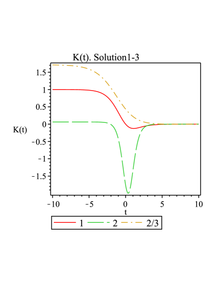
Figure 1: The total kinetic energy evolution

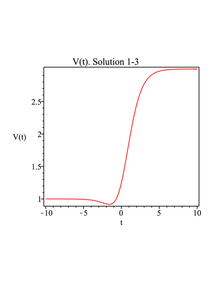
Figure 2: Evolution of the potential

For the total potential we have at the asymptotes $t\rightarrow\pm\infty$ and zero time value:

$${V_{tot}}_{(t=-\infty)}=2\textsc{K}_{(t=-\infty)}=\frac{2}{a_{i}^{2}}$$ (24)

$${V_{tot}}_{(t=0)}=\left(\frac{m\alpha^{2}(3m+\beta)}{(\beta+1)^{2}}+\frac{2\beta^{2m}}{a_{i}^{2}(\beta+1)^{2m}}\right)$$ (25)

$${V_{tot}}_{(t=+\infty)}=3m^{2}\alpha^{2}$$ (26)

For the special choice of parameters, we have a local minimum for negative time (Fig.2).

3.2 Evolution of the equation of state

Let us consider the general evolution of the EOS for the EmU scenario. With the definition of the scale factor (17), one can find

$$w_{tot}=\frac{p}{\rho}=\frac{\textsc{K}-V_{tot}}{\textsc{K}+V_{tot}}$$

Let us consider the asymptotes. At times when $t\rightarrow-\infty$ the EOS has the limiting form:

$$w_{tot}(-\infty)=-\frac{1}{3}$$ (27)

When $t\rightarrow 0$ one can easily obtain a general formula for the EOS. We will consider the result with the assumptions that $m=1$ and $\beta=1$. In this case we have:

$$w_{tot}(0)=-\frac{5\alpha^{2}a_{i}^{2}+1}{3\alpha^{2}a_{i}^{2}+3}.$$ (28)

This give us an EOS close to $-1$, if $\alpha^{2}a_{i}^{2}$ is of the order of unity.

The case $t\rightarrow+\infty$ gives us the direct answer that

$$w_{tot}(+\infty)=-1.$$

This means that at late times the Universe turns to the $\Lambda$ dark energy scenario.

This analysis confirms that it is the dark energy fields that give rise to the EmU scenario.

3.3 The number of e-foldings

In our work we have obtained exact solutions which gives us the possibility to use exact inflation techniques [21] instead of the slow-roll approximation.

Let us follow the prescription for the superpotential construction in the case of a canonical single scalar field [22]. If we choose the superpotential as the total energy potential in the form

$$\textsc{W}=V+\textsc{K}=V+\frac{1}{2}h_{11}\dot{\varphi}^{2}(t)+\frac{1}{2}h_{22}(t)\dot{\psi}^{2}(t)$$ (29)

then the linear combination of the equations for the chiral fields leads to the following relation

$$3H\left(h_{11}\dot{\varphi}^{2}(t)+h_{22}(t)\dot{\psi}^{2}(t)\right)=-\frac{d\textsc{W}}{dt}$$ (30)

This relation allows us to calculate the e-folding number for each exact solution with the formula

$$\textsc{N}=-\int_{t_{i}}^{t_{f}}\frac{\textsc{W}-\frac{\epsilon}{a^{2}}}{\frac{d\textsc{W}}{dt}}\left(2\textsc{K}\right)dt$$ (31)

As we have two fields depending on cosmic time $t$, it will be easier to integrate over $t$. Numerical integration in (31) may also be applied.

Let us mention here that for the power spectrum and spectral indexes analysis, the exact inflation approach [21] can be applied for the model under consideration as well.

Now we will present three models based on asymptotic solutions when $t\rightarrow\pm\infty$ and $V_{3}(\psi)$ tends to zero (15), and one exact solution describing the global evolution of the EmU. These solutions have been obtained with the use of the freedom in choice of the chiral metric component $h_{22}$, viz., we consider the case when the first chiral field $\varphi$ corresponds to the second term in eq. (13), i.e., we set

$$\frac{1}{2}h_{11}\dot{\varphi}^{2}(t)=-\frac{1}{\kappa}\dot{H}$$ (32)

From this relation it is easy to see that since $\dot{H}>0$ for the EmU scenario, we need $h_{11}<0$. Without loss of generality we can choose gaussian coordinates with $h_{11}=-1.$ This means that the first chiral field should be a phantom one. We connect the second chiral field with the curvature of the Universe, viz., we set

$$\frac{1}{2}h_{22}(t)\dot{\psi}^{2}(t)=\frac{1}{\kappa}\left[\frac{\epsilon}{a^{2}}\right].$$ (33)

In the case of the EmU, we obtain $h_{22}>0$, i.e., the second chiral field $\psi$ should be considered as an ordinary (canonical) field.

4 The Model  1

For simplicity, let us choose the Newton gravitational constant $\kappa=1$. Thus by integrating equation (32), we obtain for the first (phantom!) field the solution:

$$2\sqrt{2m}\tilde{\varphi}:=(\varphi(t)-\varphi_{i})=2\sqrt{-2mh_{11}}\arctan\left(\frac{e^{\frac{\alpha}{2}t}}{\sqrt{\beta}}\right)=2\sqrt{2m}\arctan\left(\frac{e^{\frac{\alpha}{2}t}}{\sqrt{\beta}}\right),$$ (34)

where $\varphi_{i}$ stands for the value of the scalar field at the time $-\infty$ . We will restrict our consideration to the period $-\frac{\pi}{2}<\tilde{\varphi}<\frac{\pi}{2}$ which allows for the time to run from $-\infty$ to $+\infty$. Let us remember that we can represent the parameter $A$ as the combination of $a_{i}$ (initial size of the EmU), and parameters $\beta$ and $m$ from the following relation: $A=\frac{a_{i}}{\beta^{m}}$. Let us note also that the solution (34) is valid for all four models.

The evolution of the second canonical field can be considered as given. Then we can calculate the chiral metric component $h_{22}$ from (33). For the first model we choose the dependence of $\psi$ on cosmic time as follows

$$\tilde{\psi}=\psi(t)-\psi_{i}=\frac{\sqrt{2}}{\zeta}e^{\zeta t},~{}~{}\zeta={\rm const},$$ (35)

Then the chiral metric component $h_{22}$ can be expressed in the form:

$$h_{22}(\tilde{\varphi})=\frac{1}{a_{i}^{2}}\left[\beta\tan^{2}\left(\frac{\varphi(t)-\varphi_{i}}{2\sqrt{2m}}\right)\right]^{-\frac{2\zeta}{\alpha}}\cos^{4m}\left(\frac{\varphi(t)-\varphi_{i}}{2\sqrt{2m}}\right)=\frac{1}{a_{i}^{2}}\left(\beta\tan^{2}(\tilde{\varphi})\right)^{-\frac{2\zeta}{\alpha}}\cos^{4m}(\tilde{\varphi}),$$ (36)

The $V_{1}$ part of the potential takes the form:

$$V_{1}(\varphi)=\frac{m\alpha^{2}}{4}\sin^{2}(2\tilde{\varphi})[3m\tan^{2}(\tilde{\varphi})+1].$$ (37)

It is worth stressing here that the solution for $V_{1}$ (37), as well as for $\tilde{\varphi}$ (34), are valid for all models below. The dependence of the shape of the potential $V_{1}$ vs $\tilde{\varphi}$ related to the parameter $m$ value is displayed in Fig. 3 and Fig. 4.

We will consider the $V_{2}$ part of the potential in the limiting case when $t\rightarrow\pm\infty$. Thus $V_{2}$ and its multiplier are:

$$f(\varphi)=\frac{1}{2}\ln\left(h_{22}(\varphi)\right),\quad$$ (38)

$$V_{2}(\psi)=\frac{2\beta^{m}}{a_{i}}\frac{\left(\frac{\zeta}{\sqrt{2}}\tilde{\psi}\right)}{\left[\beta+\left(\frac{\zeta}{\sqrt{2}}\tilde{\psi}\right)^{\frac{\alpha}{\zeta}}\right]^{m}},$$ (39)

Let us investigate the case of positive and negative $\zeta$. For the sake of simplicity let $\zeta=1$.

The general features of $h_{22}$ are as follow (see Fig.5). We consider $h_{22}$ as an even function to prevent a crossing of the phantom boundary (this case may be studied separately). During times when $t\rightarrow\pm\infty$, the chiral metric component $h_{22}\rightarrow 0$. This can be interpreted as the absence of influence from the second chiral field at the mentioned stages (as one can see in spite of the growth of the second field itself). Nevertheless during times close to zero, the value of $h_{22}$ tends to infinity. This means that the second field $\psi$ plays an important role during the inflationary period and acts as the inflaton.

The second possibility is $\zeta=-1$.

The situation in this case is different (see Fig. 6). During the inflationary stage, when time tends to zero, $h_{22}$ tends to zero and almost cancels the influence of the second field $\psi$ during times close to zero. This means that the first chiral field $\varphi$ acts as the inflaton. During the period when time tends to $\pm\infty$, the chiral metric component $h_{22}$ takes maximum values. This means that the second field $\psi$ plays an important role at infinite times.

There is one more possibility to have a solution with two maximums and one minimum by matching parameters of the model. Then $h_{22}$ tends to zero, when $t\rightarrow\pm\infty$ and $t\rightarrow\pm 0$. Thus the effect of the second field $\psi$ is cancelled during those times.

Let us turn our attention to the potential $V_{1}(\varphi)$. Its behavior looks like the case of $h_{22}$ with $\zeta=-1$ in Fig.6. The difference is in the amplitude.

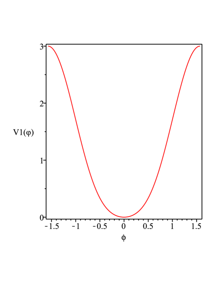
Figure 3: The potential vs the field $\varphi$, with parameters: m=1, $\alpha=1$

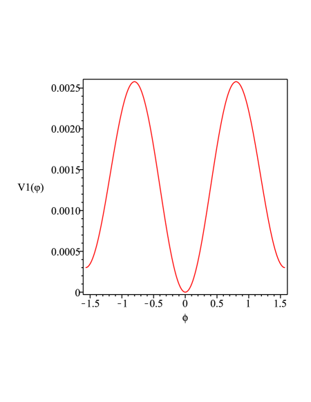
Figure 4: The potential vs the field $\varphi$, with parameters: m=0.01, $\alpha=1$

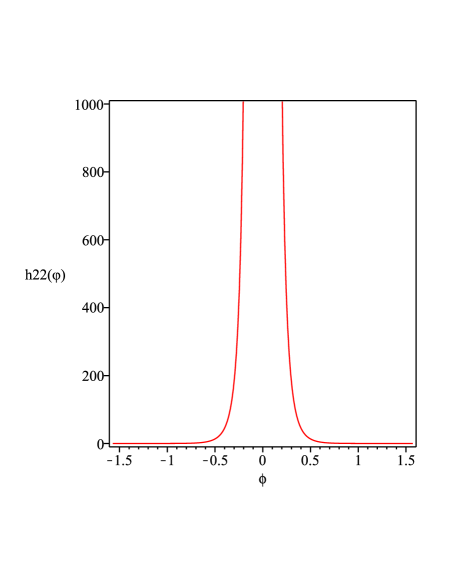
Figure 5: Model 1. The $h_{22}(\varphi)$ component vs the field $\varphi$ with parameters: A=1, m=1, $\alpha=1$, $\beta=1$, $\zeta=1$

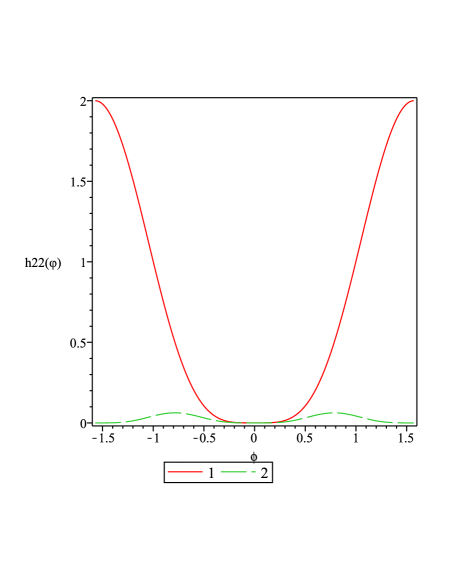
Figure 6: Model 1. The $h_{22}(\varphi)$ component vs the field $\varphi$ with $\zeta=-1$ and parameters changing

5 The Model  2

The model 1 obeys the property that the value for the second chiral field $\psi$ tends to infinity in the infinite future. From the point of view of background dark sector fields [20], it is preferable that the values of the fields are restricted. Therefore we are looking for the solution of a kink type for chiral fields. Model 2 gives us such a solution. We will keep the solution for the chiral field $\tilde{\varphi}$ in the same form as in eq. (34) as well as the solution for the $V_{1}$ part of the potential (37). This is possible because of our choice to keep for the first chiral field the responsibility for the spatially-flat part of the Universe. Let us mention once more that in the EmU, the first chiral field should be a phantom one because of relation $h_{11}\dot{\varphi}^{2}=-\dot{H}$ and the fact that $\dot{H}>0$ for the scale factor (17). We can also state that the $V_{1}$ part of the potential is determined by the spatially-flat part of the Universe. When the multiplier $e^{f(\varphi)}$ is fixed, we have a dependence of the $V_{2}$ part of the potential on the second field $\psi$.

The solutions obtained for model 2 are

$$K_{1}\tilde{\psi}:=\psi(t)-\psi_{i}=K_{1}\arctan\left(\lambda t\right)$$ (40)

$$h_{22}=\frac{2}{a_{i}^{2}K_{1}^{2}\lambda^{2}}\cos^{4m}(\tilde{\varphi})\left[1+\frac{\lambda^{2}}{\alpha^{2}}\ln^{2}(\beta\tan^{2}\tilde{\varphi})\right]^{2}$$ (41)

where $K_{1}$ is an arbitrary constant. The potential $V_{2}(\psi)$ once again in the limiting cases $t\rightarrow\pm\infty$, after some calculations, takes the form

$$V_{2}=\frac{\sqrt{2}\beta^{m}\lambda K_{1}}{a_{i}}\cos^{2}(\tilde{\psi})\left[\beta+\exp\left(\frac{\alpha}{\lambda}\tan\tilde{\psi}\right)\right]^{-m}$$ (42)

We can see from Fig. 7 and Fig. 8 the possible types of the $h_{22}$ evolution. The first possibility in Fig. 7 gives us a good example of a singularity-free solution. The influence of the second field at infinite times (past and future infinity) tends to zero, i.e., the dynamics of the Universe is determined by the first (phantom) field $\varphi$. During the inflationary period, the role of the second field $\psi$ became essential. The shape of the chiral metric component $h_{22}$ displayed in Fig. 8 provides us with some other information about the second field, viz., the field $\psi$ plays an important role at infinite times and during the inflationary period where $h_{22}$ tends to infinity.

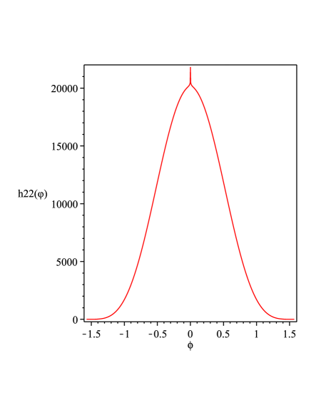
Figure 7: Model 2. The $h_{22}(\varphi)$ component vs the field $\varphi$ with parameters: A=1, K=1, m=1, $\alpha=1$, $\beta=1$, $\lambda=0.01$

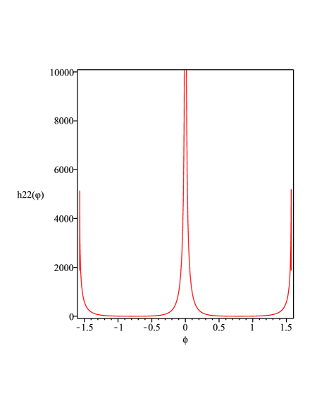
Figure 8: Model 2. The $h_{22}(\varphi)$ component vs the field $\varphi$ with parameters: A=1, K=1, m=0.1,$\alpha=1$, $\beta=1$, $\lambda=1$

6 The Model  3

As we mentioned earlier, model 1 allows infinite values for the second chiral field $\psi$. From the position of background dark sector fields [20], it would be more suitable if the values of the fields could be restricted. Therefore we seek solutions of the kink type for chiral fields. Model 2 gives us such a solution. Let us consider the solution for the chiral field $\tilde{\varphi}$ in the same form as in eq. (34)

$$2\sqrt{2m}\tilde{\varphi}:=\varphi(t)-\varphi_{i}=2\sqrt{2m}\arctan\left(\frac{e^{\frac{\alpha}{2}t}}{\sqrt{\beta}}\right),$$ (43)

The same result holds for the $V_{1}$ part of the potential, viz.,

$$V_{1}(\varphi)=\frac{m\alpha^{2}}{4}\sin^{2}(2\tilde{\varphi})[3m\tan^{2}(\tilde{\varphi})+1],$$ (44)

As a possible evolution of the second (canonical) chiral field we can consider a few possibilities, firstly, connected with the solution investigated in model 1. To avoid an infinite increase of the solution (35) when $t\rightarrow\pm\infty,$ let us choose

$$K_{1}\tilde{\psi}:=\psi(t)-\psi_{i}=K_{1}\arctan\left(\frac{\sqrt{2}}{\zeta}e^{\zeta t}\right)$$ (45)

where $K_{1}$ is arbitrary constant.

With the choice (45), the chiral metric component $h_{22}$ can be expressed in the form:

$$h_{22}(\tilde{\varphi})=\frac{1}{a_{i}^{2}K_{1}^{2}}\left[1+\frac{2}{\zeta^{2}}\left(\beta\tan^{2}\tilde{\varphi}\right)^{\frac{2\zeta}{\alpha}}\right]^{2}\left[\beta\tan^{2}\tilde{\varphi}\right]^{-\frac{2\zeta}{\alpha}}\cos^{4m}\tilde{\varphi},$$ (46)

After some calculations, we can find the $V_{2}$ part of the potential as

$$V_{2}=\frac{K_{1}\zeta\beta^{m}}{\sqrt{2}a_{i}}\sin 2\tilde{\psi}\left[\beta+\left(\frac{\zeta}{\sqrt{2}}\tan\tilde{\psi}\right)^{\frac{\alpha}{\zeta}}\right]^{-m}$$ (47)

The function $f(\varphi)$ is determined by the same relation (38):$f(\varphi)=\frac{1}{2}\ln\left(h_{22}(\varphi)\right).$

The component $h_{22}$ may have a very different shape depending on the parameters of the model. We can find shapes similar to that for model 2. But here we can find the chiral metric component $h_{22}$ in principally new forms, displayed in figures 9-10 which show the possible dependence on $\varphi$.

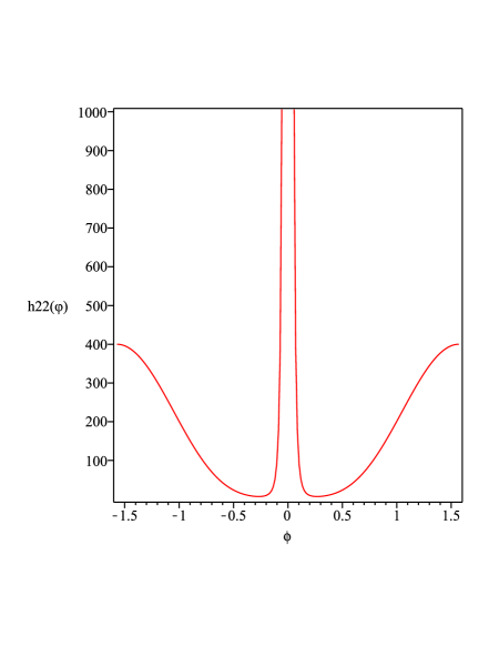
Figure 9: Model 3. The $h_{22}(\varphi)$ component vs the field $\varphi$ with parameters: A=1, K=1, m=1,$\alpha=1$, $\beta=10$, $\zeta=1$

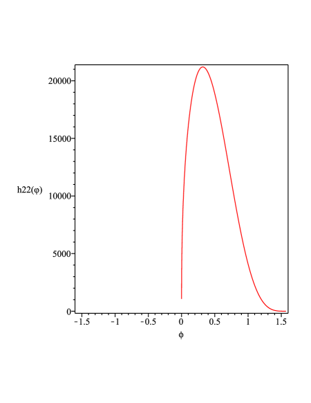
Figure 10: Model 3. The $h_{22}(\varphi)$ component vs the field $\varphi$ with parameters: A=1, K=1, m=1,$\alpha=1$, $\beta=1$, $\zeta=0.1$

7 The Model  4

We have considered solutions which are valid for times $t\rightarrow\pm\infty$. To connect the results with the entire evolution of the universe, we need an exact solution for the model. An example of such a solution can be found with the assumption that the second canonical field $\tilde{\psi}$ is proportional to the cosmic time $t$, viz., if we choose $\tilde{\psi}=\sqrt{2}t$, then we have the same solution for the first phantom field $\tilde{\varphi}$ (34) and the $V_{1}$ part of the potential (37). The $V_{3}$ part of the potential vanishes. Thus the exact solution which is valid for the entire evolution of the Universe reads

$$2\sqrt{2m}\tilde{\varphi}:=\varphi(t)-\varphi_{i}=2\sqrt{2m}\arctan\left(\frac{e^{\frac{\alpha}{2}t}}{\sqrt{\beta}}\right),$$ (48)

$$V_{1}(\varphi)=\frac{m\alpha^{2}}{4}\sin^{2}(2\tilde{\varphi})[3m\tan^{2}(\tilde{\varphi})+1],$$ (49)

$$\tilde{\psi}=\sqrt{2}t$$ (50)

$$h_{22}(\varphi)=\frac{[\cos^{2}(\tilde{\varphi})]^{2m}}{a_{i}^{2}}$$ (51)

$$V_{2}(\psi)=\frac{2}{A(\beta+e^{\frac{\alpha\tilde{\psi}}{\sqrt{2}}})^{m}},~{}~{}~{}V_{3}(\psi)=0$$ (52)

Let us compare the asymptotes of exact model 4 with the models 1-3. When $t\rightarrow+\infty$ we can state that for the exact model $h_{22}$ and $V_{2}$ tend to zero. We can find the same asymptote under special choices of parameters for the model 1 (see Fig. 5 and Fig. 6), for the model 2 (see Fig.7) and for the model 3 (see Fig. 10). As for the negative time asymptote $t\rightarrow-\infty$, we have $h_{22}\rightarrow 0$ which agrees with models 1-3, but for $V_{2}$ we have $V_{2}\rightarrow\frac{2}{a_{i}}$. The last asymptote does not exist for models 1-3. The potential part $V_{2}$ can tend to zero or to infinity.

8 Discussions

In this article, the ideas presented in the work [10] have been further developed. In [10], we considered the simplified equations for the two component nonlinear sigma model during the time when $t\rightarrow-\infty$ and also the simplified metric of the EmU during the inflationary period. Here we have presented models 1-3 with asymptotic solutions for positive and negative infinite times and model 4 which contains the exact solution with two chiral fields as some kind of dark sector fields. Model 4 describes the EmU from $t\rightarrow-\infty$ until the end of inflation, and coincides with the asymptotes of models 1-3 for those times.

If we compare the solutions obtained in the present article with those presented in [10], it becomes clear that asymptotically they may coincide under a suitable choice of the initial values for the first chiral field. But for the chiral metric component $h_{22}$ and for the second chiral field $\psi$ the results are very different. Component $h_{22}$ tends to a constant value when $t\rightarrow-\infty$, while $\psi\rightarrow-\infty$ as well. This is not very clear from a physical point of view: in the infinite past there exists a scalar field with the amplitude tending to minus infinity.

We can see another feature from the explicit solution presented in [2] for a scalar field singlet. We mention here that the exact solutions for the EmU obtained by the authors in [2] with the help of the fine turning method of the potential was suggested for the fist time in the work [24] and then developed in the works [23], [25]. Afterwards, this method was reopened in the work [26] and applied to tachyonic matter.

The solution in [2] consists of two parts: asymptotically a static Einstein Universe when $t\rightarrow-\infty$ and at late times the scale factor has exponential behavior $a(t)\propto\exp(\alpha t)$.

If we consider the solutions for the potential and the scalar field, we find an unpleasant situation with the scalar field: it tends to $-\infty$, and the potential tends to a constant value. We have the same situation with the $V_{1}$ part of the potential for the models 1-3 presented in this article. For the model 1, we have constant values for $t\rightarrow-\infty$ and an infinite increase of the second field for $t\rightarrow\infty$. But for model 2 and model 3 this unpleasant behavior was corrected. Thus we suggested models which are reasonable from a physical point of view: the chiral fields (the first is phantom one, while the second is canonical) are evaluated during the global evolution of the Universe and they are restricted in amplitudes. The kinetic interaction between these two fields has the feature that during the inflationary stage they may have infinite values. This fact may be interpreted as a dominant influence of the second canonical scalar field during the inflationary stage. Nevertheless, for a special choice of parameters, the amplitude of the second field may have a large but finite value.

Let us stress here that we have obtained for the first time an exact solution for the EmU supported by two chiral fields in model 4. When $t\rightarrow-\infty$ we have $\psi\rightarrow-\infty$, the chiral metric component $h_{22}\rightarrow 0$ and the $V_{2}$ part of the potential tends to the constant: $V_{2}\rightarrow\frac{2}{a_{i}}$. Nevertheless, if we take into account the multiplier $e^{f(\varphi)}=\sqrt{h_{22}}$ of the $V_{2}$ which tends to zero, effectively the situation will be as in the case of models 1-3. When $t\rightarrow+\infty$, we have $\psi\rightarrow+\infty$ and the chiral metric component $h_{22}$ and the $V_{2}$ part of the potential tend to zero which is in agreement with models 1-3.

Summing up the result of the article we can state that the exact solutions of the model 4 we found here can support the EmU during the entire evolution of the Universe, starting from the infinite past and evolving to the end of inflation with the necessary emergence from the inflationary stage in the usual way: decay of scalar fields, particle production, reheating etc. Moreover, we investigated the role of the chiral metric component $h_{22}$ responsible for the interaction of the first phantom chiral field and the second canonical field.

9 Acknowledgments

SC is thankful to the University of KwaZulu-Natal, the University of Zululand and the NRF for financial support and warm hospitality during his visit in 2011 to South Africa. SDM acknowledges that this work is based upon research supported by the South African Research Chair Initiative of the Department of Science and Technology and the National Research Foundation.

References

- [1] Ellis G F R and Maartens R 2002 The emergent universe: inflationary cosmology with no singularity Class. Quant Grav. 21, 223-232, arXiv: gr-qc/0211082
- [2] Ellis G F R, Murgan J and Tsagas C 2004 The emergent universe: an explisit construction Class.Quant.Grav. 21, 233-250, arXiv: gr-qc/0307112
- [3] Marylyne D J, Tavakol R, Lidsey J E and Ellis G R F 2005 An emergent universe from a loop arXiv: astro-ph/0502589
- [4] Mukherjee S, Paul B S, Maharaj S D and Beesham A 2005 Emergent universe in Starobinsky model arXiv: gr-qc/0505103
- [5] Banerjee A, Bandyopadhyay T and Chakraborty S 2007 Emergent universe in Brane World Scenario arXiv: 0705.3933 [gr-qc]
- [6] Banerjee A, Bandyopadhyay T and Chakraborty S 2007 Emergent universe in Brane World Scenario with Schwarzschild-de Sitter Bulk arXiv: 0711.4188 [gr-qc]
- [7] Liddle A R and Lyth D H 1993 Phys. Rep. 1, 231
- [8] Chervon S V 1995 Izv.Vyssh.Ucheb.Zaved. Fiz. 5, 114
- [9] Tsujikawa S 2010, Dark Energy: investigations and modelling, ArXiv:1004.1493
- [10] Beesham A, Chervon S V, Maharaj S D 2009, Emergent Universe supported by Non-linear Sigma Model Class. Quantum Grav. 26 075017
- [11] Chervon S V 1995, Chiral non-linear sigma models and cosmological inflation// Gravitation & Cosmology, Vol.1, No.2, p.91
- [12] Chervon S V 1997, Gravitational Field of the Early Universe I: Non-linear scalar field, Gravitation. & Cosmology 3, 145
- [13] Chervon S V 2002, A Global Evolution of the Universe Filled by Scalar or Chiral Fields// Gravitation & Cosmology. 3, 32
- [14] Chervon S V 2001, Exact solutions in standard and chiral inflationary models//Proceedings of 9th Marcell Grossman Conference, Roma, 2000. World Scientific, p.1909, Pt.C.
- [15] Chervon S V 1997, Non-Linear Fields in the Theory of Gravitation and Cosmology, Ulyanovsk State University, Ulyanovsk, 191
- [16] Mukherjee S, Paul B S, Dadhich N K , Maharaj S D and Beesham A 2006 Emtrgent universe with exotic matter Class.Quant.Grav., 23, 6927
- [17] Paul B C, Thakur P, Ghose S 2010 Constraint on exotic matter needed for an emergent universe, Mon. Not. Roy. Astron. Soc., arXiv: 1004.4256
- [18] Debnath U 2008 Emergent universe and phantom tachyon model, Class. Quant. Grav., 25, 205019 arXiv:0808.2379
- [19] Chattopadhay S, Debnath U, 2011 Emergent universe in chameleon, f(R) and f(T) gravity theories, Int.J.Mod.Phys.D20, 1135-1152 arXiv: 1105.1091
- [20] Chervon S V, Panina O G 2010 Effects of stiff influence dark sector fields on cosmological perturbations Journal ”Vestnik RUDN” ? 4. (In Russian).
- [21] Chervon S V, Fomin I V 2008 On Calculation of the Cosmological Parameters in Exact Models of Inflation. Gravitation & Cosmology, 14, 2, 163-167
- [22] Yurov A V, Yurov V A, Chervon S V, Sami M 2011 Potential of total energy as superpotential in integrable cosmological models. Theor. and Math. Phys. 166(2), 258-268
- [23] Chervon S V , Zhuravlev V M and Shchigolev V K 1997 Phys. Lett. B 398, 269.
- [24] Ellis G R F, Madsen M S 1991 Class. Quantum Grav. 8, 667
- [25] Zhuravlev V M, Chervon S V and Shchigolev V K 1990 JETF, 87, 223
- [26] Padmanabhan T. ArXiv:hep-th/0204415