First principles molecular dynamics without self-consistent field optimization

Abstract

We present a first principles molecular dynamics approach that is based on time-reversible extended Lagrangian Born-Oppenheimer molecular dynamics [Phys. Rev. Lett. 100, 123004 (2008)] in the limit of vanishing self-consistent field optimization. The optimization-free dynamics keeps the computational cost to a minimum and typically provides molecular trajectories that closely follow the exact Born-Oppenheimer potential energy surface. Only one single diagonalization and Hamiltonian (or Fockian) construction are required in each integration time step. The proposed dynamics is derived for a general free-energy potential surface valid at finite electronic temperatures within hybrid density functional theory. Even in the event of irregular functional behavior that may cause a dynamical instability, the optimization-free limit represents a natural starting guess for force calculations that may require a more elaborate iterative electronic ground state optimization. Our optimization-free dynamics thus represents a flexible theoretical framework for a broad and general class of ab initio molecular dynamics simulations.

I Introduction

The molecular dynamics simulation method based on first principles electronic structure theory is rapidly emerging as a powerful and almost universal tool in materials science, chemistry and molecular biology Marx and Hutter [2000], Kirchner [2012]. A few early applications of Born-Oppenheimer molecular dynamics date back four decades ago Wang and Karplus [1973], Leforestier [1978] and highly efficient density functional methods Hohenberg and Kohn [1964], Kohn and Sham [1965] using plane-wave pseudopotential techniques and the fast Fourier transform Cooley and Tukey [1965] appeared already in the mid 80’s and early 90’s Car and Parrinello [1985], Remler and Madden [1990], Vanderbilt [1990], Payne et al. [1992], Kresse [1993], Barnett [1993]

One of the major computational obstacles in first principles Born-Oppenheimer molecular dynamics simulations is the iterative, non-linear, self-consistent field optimization that is required prior to the force calculations Remler and Madden [1990], Pulay and Fogarasi [2004], Marx and Hutter [2000]. Many methods have been proposed to overcome this fundamental problem Car and Parrinello [1985], Payne et al. [1992], Arias et al. [1992], Hartke [1992], Schlegel [2001], Tuckerman [2002], Schlegel [2002], Herbert [1992], Pulay and Fogarasi [2004], Niklasson et al. [2006], Kühne et al. [2006], Alonso [2008], Jakowski [2009]. One of the more recent approaches is based on an extended Lagrangian formulation of a time-reversible Born-Oppenheimer molecular dynamics Niklasson [2008], Steneteg et al. [2010], Zheng et al. [2011], Hutter [2012], Lin et al. [2013], which reduces the computational cost of the self-consistent field optimization while keeping the dynamics stable with respect to long-term energy conservation. Extended Lagrangian Born-Oppenheimer molecular dynamics can be used both for metallic and non-metallic materials Steneteg et al. [2010], Lin et al. [2013], Niklasson et al. [2011], the integration time step is governed by the slower nuclear degrees of freedom, and it can be used in combination with fast (non-variational) linear scaling electronic structure solvers without causing a systematic drift in the energy Cawkwell and Niklasson [2012]. It has further been argued that extended Lagrangian Born-Oppenheimer molecular dynamics provides a general theoretical framework for alternative forms of first principles molecular dynamics methods Hutter [2012].

The purpose of this paper is to explore some limits of the extended Lagrangian formulation of Born-Oppenheimer molecular dynamics. Our main focus is a generalization in the limit of vanishing self-consistent field optimization. This generalization has previously been investigated within self-consistent-charge tight-binding and Hartree-Fock theory Niklasson and Cawkwell [2012], Souvatzis and Niklasson [2013]. In this paper we further extend and explore the optimization-free limit to free-energy potential surfaces valid also at finite electronic temperatures within a general hybrid density functional theory. Our proposed optimization-free dynamics requires only one diagonalization and in contrast to previous Hartree-Fock simulations Souvatzis and Niklasson [2013] also only one single effective Hamiltonian construction per time step. This is a significant improvement over the previous Hartree-Fock calculations, which is made possible by using a particular linearized expression for the potential free energy. This formulation also provides a computationally simple force expression that is fully compatible with the potential energy. For normal simulations that do not encounter irregular (non-convex) behavior in the functional form around the self-consistent ground state, the optimization-free dynamics yields trajectories that are practically indistinguishable from an ”exact” Born-Oppenheimer molecular dynamics simulation. However, in the event of anomalous behavior that may cause numerical instabilities, the optimization-free limit nevertheless also represents a natural and efficient starting guess for more elaborate force calculations that require an iterative and improved accuracy in the electronic ground state optimization or reduced integration time steps to recover stability Lin et al. [2013], Niklasson et al. [2009], Steneteg et al. [2010]. The proposed optimization-free limit of extended Lagrangian Born-Oppenheimer molecular dynamics therefore represents a flexible theoretical framework for a very broad and general class of materials simulations.

II Time-reversible Extended Lagrangian Born-Oppenheimer molecular dynamics

Extended Lagrangian Born-Oppenheimer molecular dynamics Niklasson [2008], Steneteg et al. [2010], Zheng et al. [2011] enables a time-reversible integration of the equations of motion that improves the long-term stability of a molecular dynamics simulation, while keeping the computational cost low by reducing the number of required self-consistent field iterations. In our presentation below we will use density matrices for the electronic degrees of freedom, which is a natural choice for hybrid functionals, i.e. that is easily applicable both in Hartree-Fock Roothaan [1951], McWeeny [1960] and density functional theory Parr and Yang [1989], Dreizler and Gross [1990]. However, the approach is quite general and should be straightforward to apply also to wavefunctions and the electron density Steneteg et al. [2010], Zheng et al. [2011].

In our discussion we will use the term “ground state” density matrix and “Born-Oppenheimer” molecular dynamics also for finite temperature ensembles with thermally excited states Parr and Yang [1989]. We use these terms since the self-consistent, fractionally occupied, (i.e. non-idempotent) density matrix minimizes a free energy functional that represents a straightforward generalization of regular Born-Oppenheimer molecular dynamics that is valid both at zero and finite electronic temperatures Niklasson et al. [2011].

The finite temperature generalization provides a useful tool for simulations of, for example, metals and warm dense matter, or simply as an ad hoc tool to avoid self-consistent field instabilities.

II.1 With self-consistent field optimization

In time-reversible extended Lagrangian Born-Oppenheimer molecular dynamics the regular dynamical variables for the nuclear degrees of freedom are extended with an auxiliary dynamical variable for the electronic degrees of freedom, $P$, that evolves close to the optimized self-consistent electronic ground state density matrix, $D$. The extended Lagrangian equations of motion for the nuclear coordinates, $\{R_{I}\}={\bf R}$, for a general free energy potential surface, $\Omega$, that are valid also at finite electronic temperatures are given by

$${\displaystyle M_{I}{\ddot{R}}_{I}=-\frac{\partial\Omega[{\bf R},D]}{\partial R_{I}}},$$ (1)

where the dots denote time derivatives. The equations of motion can be integrated, for example, with the regular velocity Verlet algorithm using Hellmann-Feynamn and Pulay forces Feynman [1939], Marx and Hutter [2000], Pulay [1969], Niklasson et al. [2011]. The extended Lagrangian equation of motion for the extended auxiliary electronic dynamical variable, $P$, is given by a harmonic oscillator centered around the self-consistent electronic ground state density matrix, $D$, where

$${\displaystyle{\ddot{P}}=\omega^{2}(D-P)}.$$ (2)

Since $P(t)$ evolves in a harmonic well that follows the ground state, $D(t)$, the dynamical variable $P(t)$ will stay close to the ground state for sufficiently large values of the frequency parameter $\omega$ or small integration time steps $\delta t$. Moreover, since $P(t)$ is a dynamical variable it can be integrated with a time-reversible or symplectic integration scheme Niklasson [2008], Niklasson et al. [2009], Odell et al. [2009, 2011]. In this way we can use $P(t+\delta t)$ as an accurate initial guess to the self-consistent-field (SCF) optimization procedure of the ground state density matrix, where

$$D(t+\delta t)={\rm SCF}[P(t+\delta t)],$$ (3)

without breaking time reversibility in the underlying electronic degrees of freedom. It is thanks to this time-reversibility that the long-term conservation of the total energy is stabilized in extended Lagrangian Born-Oppenheimer molecular dynamics even under approximate and incomplete self-consistent field convergence.

The free energy potential, $\Omega$ in Eq. (1), is here given by

$$\Omega[{\bf R},D]=E[D]-T_{e}{\cal S}[D]+U^{\rm pair}({\bf R}),$$ (4)

where $E-T_{e}{\cal S}$ is the electronic free energy at electronic temperature $T_{e}$ with an electronic energy, $E$, and an entropy term, ${\cal S}$. $U^{\rm pair}$ is a pair potential term including ion-ion repulsions and, for example, Van der Waals corrections. The electronic energy term, $E$, is here assumed to be described by a (restricted) general hybrid density functional expression, with

$$E[D]=2Tr[hD]+Tr[DG^{\alpha}(D)]+E^{xc}[2D].$$ (5)

The matrix $h$ corresponds to the one-electron integrals and $G^{\alpha}(D)$ are the regular Coulomb, $J$, and exchange, $K$, matrices in Hartree-Fock theory Roothaan [1951], McWeeny [1960], with the exchange matrix $K$ scaled by a factor $\alpha$ to account for hybrid functionals, i.e.

$$G^{\alpha}(D)=2J(D)-\alpha K(D).$$ (6)

The exchange correlation term $E^{xc}[2D]$ can be a gradient corrected expression PBE , a local density approximation LDA , or other mixed functional expressions B3LYP , with the electron density given by the (doubly occupied) density matrix, i.e. $2D$. The ground state density matrix, $D$, which determines the potential energy surfaces for the inverse temperature $\beta=1/(k_{B}T_{e}$), is given by the self-consistent condition

$$D^{\perp}=\left[e^{\beta\left(H^{\perp}(D)-\mu_{0}I\right)}+1\right]^{-1},$$ (7)

where the effective single particle Hamiltonian (or Fockian), $H$, is given by

$$H(D)=h+G^{\alpha}(D)+V^{xc}(2D).$$ (8)

The orthogonalized representation of the Hamiltonian, $H^{\perp}$, in Eq. (7) above, is calculated through the congruence transformation,

$$H^{\perp}=Z^{T}HZ,$$ (9)

where $Z$ and its transpose $Z^{T}$ are the inverse factors of the basis set overlap matrix $S$, i.e.

$$Z^{T}SZ=I,$$ (10)

and the density matrix in its non-orthogonal form is

$$D=ZD^{\perp}Z^{T}.$$ (11)

The chemical potential, $\mu_{0}$, is determined to give $D$ the correct occupation of electrons $N_{e}$, i.e. $\mu_{0}$ is set such that $N_{e}=2Tr[D^{\perp}]=2Tr[DS]$. $V^{xc}(2D)$ in Eq. (8) is the regular exchange correlation potential given through the functional derivative of the exchange correlation energy. $V^{xc}(2D)$ is a functional of the electron density given by the doubly occupied density matrix. The electronic entropy term ${\cal S}$ in Eq. (4) for the spin restricted case, i.e. with double occupation of each orbital, is

$$\begin{array}[]{l}{\cal S}[D]=-2k_{B}Tr\left[D^{\perp}\ln(D^{\perp})\right.\\ {}\\ ~{}~{}+\left.(I-D^{\perp})\ln(I-D^{\perp})\right],\end{array}$$ (12)

which makes the free energy functional variationally correct at the ground state Weinert and Davenport [1992], Wentzcovitch et al. [1992], Niklasson et al. [2011].

II.2 Without self-consistent field optimization

The major computational cost of a first principles Born-Oppenheimer molecular dynamics simulation is the iterative self-consistent field optimization that is required prior to the force calculations. If a sufficient degree of optimization is not fulfilled, the Hellmann-Feynman forces are no longer accurate Feynman [1939], Marx and Hutter [2000], Pulay [1969], Niklasson [2008b], which in regular Born-Oppenheimer molecular dynamics typically leads to a systematic drift in the total energy Remler and Madden [1990], Pulay and Fogarasi [2004], Niklasson et al. [2006]. Only by a computationally expensive increase in the number of self-consistent field iterations is it possible to reduce this drift, though it never fully disappears. This systematic error accumulation is very unfortunate since the error in each individual force calculation often is small compared to the local truncation error caused by the finite integration time step $\delta t$. The underlying time-reversibility enabled by the extended Lagrangian formulation in Eqs. (1) and (2) eliminates this problem with respect to the systematic long-term energy drift even for fairly approximate degrees of self-consistent field optimization.

In a regular leap-frog or Verlet based integration of the equations of motion, Eqs. (1) and (2), the local truncations error as measured by the amplitude of the oscillations in the total energy (kinetic + potential), scales with the square of the integration time step, i.e. as $\sim\delta t^{2}$. Without a global systematic error accumulation, the error in time-reversible extended Lagrangian based Born-Oppenheimer molecular dynamics is thus governed only by the local truncation error $\sim\delta t^{2}$. This gives us the opportunity to further relax the accuracy in the individual force calculations as long as any additional error is of the same order as the local truncation error. This would allow a reduction of the computational cost without any significant change in the level of accuracy. As in classical molecular dynamics simulations, the effect on the molecular trajectories should be no different than using a slightly longer (or shorter) integration time step. What we will demonstrate here, is that this is possible to achieve, at least under normal simulation conditions, even without any self-consistent field optimization at all prior to the force calculations. This optimization-free approach keeps the computational cost to a minimum. Only one single diagonalization and Hamiltonian construction per time step is required.

The equations of motion, Eqs. (1) and (2), provide the exact Born-Oppenheimer molecular dynamics only for the exact ground state (gs) density matrix, $D\equiv D_{\rm gs}$. Since the exact self-consistent ground state in practice never can be reached, even after multiple self-consistent field iterations, we always have some small deviation, $\delta D$, from the exact solution, i.e. in real calculations

$$D=Z\left[e^{\beta\left(H^{\perp}(D_{\rm gs}+\delta D)-\mu_{0}I\right)}+1\right]^{-1}Z^{T}.$$ (13)

Fortunately, the variational property of the electronic free energy leads to only a minor error and

$$\begin{array}[]{l}E[D]-T_{e}{\cal S}[D]=\\ {}{}\\ ~{}~{}E[D_{\rm gs}]-T_{e}{\cal S}[D_{\rm gs}]+{\cal O}((D-D_{\rm gs})^{2}).\end{array}$$ (14)

Nevertheless, because of the broken commutation between the approximate ground state density matrix $D$ and $H(D)$, the Hellmann-Feynman force expression is not valid, which in regular Born-Oppenheimer molecular dynamics leads to small but systematic errors in the forces and eventually to a significant loss of long-term accuracy. Within time-reversible extended Lagrangian Born-Oppenheimer molecular dynamic, it is possible to avoid this shortcoming, even without any self-consistent field optimization at all prior to the force calculations. We achieve this by using a particular linearized approximation of the electronic free energy, $E-T_{e}{\cal S}$. This linearization provides two important advantages compared to our previous Hartree-Fock simulations Souvatzis and Niklasson [2013]: (a) only one single Hamiltonian (or Fockian) construction is needed in each time step, and (b) the nuclear forces are computationally simple yet fully compatible with the linearlized energy expression.

Let the potential free energy be given by the linearized expression

$$\begin{array}[]{l}{\cal F}[P]=2Tr[hD]+Tr[(2D-P)G^{\alpha}(P)]\\ {}{}\\ ~{}~{}~{}~{}+E^{xc}[2D]-T_{e}{\cal S}[D],\end{array}$$ (15)

where

$$D\equiv D(P)=\left[e^{\beta\left(H^{\perp}(P)-\mu I\right)}+1\right]^{-1}.$$ (16)

It is then straightforward to show that

$$\begin{array}[]{l}{\cal F}[P]=E[D_{\rm gs}]-T_{e}{\cal S}[D_{\rm gs}]\\ {}{}\\ +{\cal O}[(D_{\rm gs}-D)^{2}]+{\cal O}[(D-P)^{2}].\\ \end{array}$$ (17)

Moreover, since $P$ is a dynamical variable, we can use a very simple “Hellmann-Feynman-like” expression for the forces including a basis-set dependent Pulay term that are given from the partial derivative of the electronic free energy (see Appendix),

$$\begin{array}[]{l}{\cal F}_{R}[P]=2Tr[h_{R}D]+Tr[(2D-P)G^{\alpha}_{R}(P)]\\ {}{}\\ ~{}~{}~{}~{}+E^{xc}_{R}[2D]+2Tr[S^{-1}H(P)DS_{R}].\end{array}$$ (18)

The last term is the basis-set dependent Pulay term, which here is generalized to finite electronic temperatures including the electronic entropy contribution Niklasson [2008b]. The main reason for this simple form of the force expression, which is valid without any self-consistent optimization of the density matrix $D$, is that the partial derivatives are with respect to a constant $P$, since it occurs as a dynamical variable. The subscript $R$ in $G^{\alpha}_{R}(P)$ and $E^{xc}_{R}[2D]$ denotes the $R_{I}$ derivatives with respect to the atomic centered underlying basis set. Only one single diagonalization and effective Hamiltonian (or Fockian) construction is needed in each time step.

The linearized expression of the general hybrid free-energy functional in Eq. (15) and the corresponding forces in Eq. (18) represent the underlying theory of this paper. A detailed derivation starting with Eq. (15) of the force expression in Eq. (18), which is valid to second order ${\cal O}[(D-P)^{2}]$, is given in the appendix.

II.3 Stability conditions for the electronic integration

In comparison to exact Born-Oppenheimer molecular dynamics, the error in both the forces and the total energy in Eqs. (15) and (18) should be no worse than of order ${\cal O}[(D_{\rm gs}-P)^{2}]={\cal O}[(D_{\rm gs}-D)^{2}]+{\cal O}[(D-P)^{2}]$, assuming ${\cal O}[(D_{\rm gs}-D)^{2}]\leq{\cal O}[(D-P)^{2}]$. The accuracy of the optimization-free dynamics above is thus governed by an error term ${\cal O}((D_{\rm gs}-P)^{2})$. It is therefore important to keep the auxiliary dynamical variable $P$ as close as possible to the ground state. Since $P$ only moves towards the exact ground state, $D_{\rm gs}$, through the harmonic oscillator centered around the approximate ground state $D$, the equation of motion for the electronic degrees of freedom, Eq. (2), which formally is derived within the extended Lagrangian framework for $D\equiv D_{\rm gs}$, will in general be unstable unless

$$\|D-D_{\rm gs}\|<\|P-D_{\rm gs}\|.$$ (19)

To enable stability in our pursued limit of only one single diagonalization per time step, we may use an approximate equations of motion for the electronic degrees of freedom,

$${\ddot{P}}=\omega^{2}({\widetilde{D}}-P),$$ (20)

where ${\widetilde{D}}$ is some improved approximation, compared to $D$, of the exact ground state, i.e.

$${\widetilde{D}}={\widetilde{D}}(D,P)\approx D_{\rm gs},$$ (21)

Possibly the simplest choice is a linear mixing where

$${\widetilde{D}}(D,P)=\gamma D+(1-\gamma)P.$$ (22)

This choice leads to the same form for the equations of motion as in (SCF-optimized) extended Lagrangian Born-Oppenheimer molecular dynamics,

$${\ddot{P}}=\gamma\omega^{2}(D-P),$$ (23)

but now with $\omega^{2}$ scaled by a constant $\gamma$. In this case, stability can be achieved whenever the functional form of ${\cal F}[P]$ is convex in the sense that there exist a constant $\gamma\in[0,1]$ such that

$${\cal F}[\gamma D+(1-\gamma)P]<\gamma{\cal F}(D)+(1-\gamma){\cal F}(P).$$ (24)

In this simple case of linear mixing, which we have used throughout all our calculations, we can therefore use the regular unoptimized equation of motion in Eq. (2), with $\Omega$ defined through ${\cal F}[P]$ in Eq. (15) and with $\omega^{2}$ rescaled by a factor $\gamma\in[0,1]$. This approach is simple and straightforward and works for normal convex functional forms. In the (rare) event of functional anomalies, for example, due to broken functional convexity with a self-consistent field instability, we may have to adjust the scaling factor $\gamma$, reduce the integration time step $\delta t$, use more advanced (preconditioned) approximations for ${\widetilde{D}}(D,P)$, introducing an ad hoc electronic thermal smearing or revert to a more costly iterative self-consistent field optimization procedure. The automatic “on-the-fly” detection and development of such adaptive integration methods is an area for future research.

An interesting analysis of stability and accuracy conditions of the equations of motion derived from extended Lagrangian Born-Oppenheimer molecular dynamics can be found in a recent paper by Lin et al. Lin et al. [2013]. This paper also includes a detailed comparison between time-reversible extended Lagrangian Born-Oppenheimer molecular dynamics and the more well-known method by Car and Parrinello Car and Parrinello [1985]. A key difference is their sensitivity to the electronic gap and thus the ability to simulate metallic systems, which is straightforward with extended Lagrangian Born-Oppenheimer molecular dynamics Steneteg et al. [2010]. Another difference is that the constant of motion in Car-Parrinello molecular dynamics includes the electronic kinetic energy. This is not the case in extended Lagrangian Born-Oppenheimer molecular dynamics, which is formally derived in the adiabatic limit of vanishing (zero) electron mass. A generalized presentation of both Car-Parrinello and extended Lagrangian Born-Oppenheimer molecular dynamics is also given in a recent paper by Hutter Hutter [2012].

II.4 Equations of motion for a fast quantum mechanical molecular dynamics

As a summary of the discussion above we have derived, based on extended Lagrangian Born-Oppenheimer molecular dynamics, a fast quantum mechanical molecular dynamics (fast-QMMD) scheme that requires only one single diagonalization and Hamiltonian construction per time step. The nuclear degrees of freedom is governed by

$${\displaystyle M_{I}{\ddot{R}}_{I}=-\left.\frac{\partial\Omega[{\bf R},P]}{\partial R_{I}}\right|_{P}},$$ (25)

and the electronic evolution by

$${\ddot{P}}=\omega^{2}\left({\widetilde{D}}-P\right)=\gamma\omega^{2}\left(D-P\right).$$ (26)

The nuclear forces in Eq. (25) are given for the partial derivatives of $\Omega$ with respect to nuclear coordinates $R_{I}$ under the condition of constant $P$. The potential energy is

$$\begin{array}[]{l}{\Omega}[{\bf R},P]=2Tr[hD]+Tr[(2D-P)G^{\alpha}(P)]\\ {}{}\\ ~{}~{}+E^{xc}[2D]-T_{e}{\cal S}[D]+U^{\rm pair}({\bf R}),\end{array}$$ (27)

with the corresponding forces

$$\begin{array}[]{l}{\Omega}_{R}[{\bf R},P]=2Tr[h_{R}D]+Tr[(2D-P)G^{\alpha}_{R}(P)]\\ {}{}\\ ~{}~{}+E^{xc}_{R}[2D]+2Tr[S^{-1}H(P)DS_{R}]+U^{\rm pair}_{R}({\bf R}).\end{array}$$ (28)

The density matrix $D$ at $T_{e}\geq 0$ is

$$D\equiv D(P)=Z\left[e^{\beta\left(H^{\perp}(P)-\mu I\right)}+1\right]^{-1}Z^{T},$$ (29)

where

$$H^{\perp}(P)=Z^{T}\left(h+G^{\alpha}(P)+V^{xc}(2P)\right)Z.$$ (30)

As above, the congruence factor $Z$ and its transpose $Z^{T}$ are determined by $Z^{T}SZ=I$, where $S$ is the basis-set overlap matrix. We integrate the nuclear degrees of freedom with a regular velocity-Verlet scheme. The electronic equation of motion, Eq. (26), is integrated with a modified Verlet scheme Niklasson et al. [2009], Steneteg et al. [2010], Zheng et al. [2011] that removes a possible accumulation numerical noise through a weak dissipation. For the linear mixing approximation of ${\widetilde{D}}$ in Eq. (22), this modified Verlet integration is

$$P_{n+1}=2P_{n}-P_{n-1}+\gamma\kappa(D_{n}-P_{n})+\alpha\sum_{k=0}^{K}c_{k}P_{n-k},$$ (31)

where the dimensionless variable $\kappa=\delta t^{2}\omega^{2}$ is rescaled by the constant $\gamma\in[0,1]$. Three material independent sets of optimized coefficients for $\alpha$ and $c_{k}$ are given in Tab. 1. Alternative higher-order symplectic integration schemes can also be applied Niklasson [2008], Odell et al. [2009, 2011], but have not been used in the present study.

Table 1: Coefficients for the Verlet integration scheme with the external dissipative force term in Eq. (31). The coefficients are derived in Ref. Niklasson et al. [2009], which contains a more complete set of coefficients.

$K$	$\delta t^{2}\omega^{2}$	​​$\alpha\!\times\!10^{-3}$​​	​$c_{0}$	$c_{1}$	$c_{2}$	$c_{3}$	$c_{4}$	$c_{5}$	$c_{6}$	$c_{7}$
5	1.82	​​18​​	-6	14	-8	-3	4	-1
6	1.84	​​5.5​​	-14	36	-27	-2	12	-6	1
7	1.86	​​1.6​​	-36	99	-88	11	32	-25	8	-1

III Examples and Analysis

The proposed fast-QMMD scheme, Eqs. (25 - 31), has been implemented in the Uppsala Quantum Chemistry code (UQuantChem) UQuantChem [2013], which is a freely available program package for ab initio electronic structure calculations using Gaussian basis set representations that can be obtained from the code’s homepage UQuantChem [2010]. The UQuantChem program includes Hartree-Fock theory, diffusion and variational Monte Carlo, configuration interaction, Moller-Plesset perturbation theory, density functional theory and hybrid functionals, finite temperature calculations, structural optimization and first principles molecular dynamics simulations. Our fast-QMMD implementation in the UQuantChem package has been carefully commented in reference to this paper in order to facilitate the implementation of the fast-QMMD scheme into a broader variety of electronic structure software. Notice, that details of the implementation are very important and it may not always be straightforward to implement the fast-QMMD scheme in a regular first principles electronic structure code.

All our “exact” Born-Oppenheimer molecular dynamics (BOMD) simulations were performed based on extended Lagrangian Born-Oppenheimer molecular dynamics, Eqs. (1) and (2), using 5 self-consistent-field optimization cycles per time step prior to the force calculations. This choice provides a convergence in the potential free energy of about $\sim 10^{-7}$ Hartree, which is 2-3 orders of magnitude smaller than the oscillations in the total energy that are used in the comparisons.

III.1 Comparison to Born-Oppenheimer molecular dynamics

In Fig. 1 we show a comparison between our fast-QMMD, Eqs. (25-31), and self-consistent Born-Oppenheimer molecular dynamics with respect to the fluctuations in the total energy (kinetic + potential), i.e. the local truncation error, for simulations of a single water molecule. We have used three different levels of density functional theory: a) the local density approximation (LDA) LDA , b) the gradient corrected approximation (PBE) PBE , and c) a hybrid functional (B3LYP) B3LYP . In all cases we find that the total energy fluctuations,

$$E_{\rm Tot}(t)=\frac{1}{2}\sum_{I}M_{I}{\dot{R}}^{2}_{I}(t)+\Omega({\bf R},t),$$ (32)

behave in a very similar way. For the fast-QMMD simulations we used the potential energy expression of $\Omega({\bf R},t)$ in Eq. (27) to estimate the total energy.

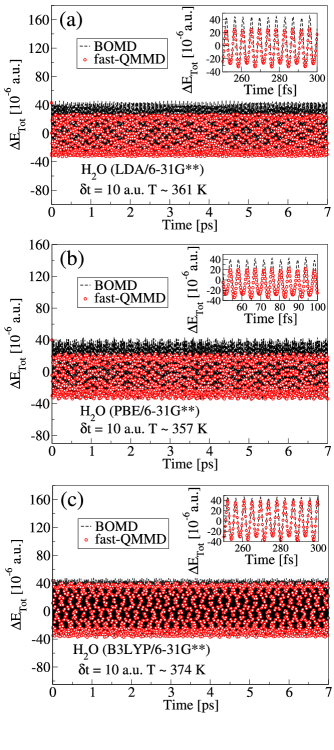
Figure 1: Total energy fluctuations (kinetic + potential) for water using self-consistent Born-Oppenheimer molecular dynamics (BOMD), and the first principles fast-QMMD, Eq. (25-31). For the fast-QMMD simulation we used the electronic free energy expression in Eq. (27) in the total energy estimates. All calculations were performed with the modified Verlet integration ($K$ = 7 in table 1) and rescaling of $\kappa=\delta t^{2}\omega^{2}$ with a factor $\gamma$ = 0.7. The time step used was 10 a.u.

In the next figure, Fig. 2 (a), we show interatomic distances between self-consistent Born-Oppenheimer molecular dynamics and our proposed fast-QMMD scheme for a C₂H₆ molecule using the local density approximation. The upper panel shows virtually no difference between the fast optimization-free scheme and the optimized “exact” Born-Oppenheimer simulation. The curves are essentially on top of each other even after 500 fs of simulation time. For any chaotic dynamical system like this, the curves will eventually diverge due to any infinitesimal perturbation. The lower panel, Fig. 2 (b), shows an example of the interatomic C-F distance in a CF₄ molecule. Here we use a four times longer integration time step, $\delta t$ = 40 a.u., and we find a small shift in the frequency that is visible after a few hundred time step. For the first 100-200 fs of simulation time the curves are very close.

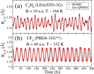
Figure 2: Interatomic distances calculated using self-consistent Born-Oppenheimer molecular dynamics (BOMD), and the first principles fast-QMMD, Eq. (25-31). In (a), the interatomic distance between the Carbon atoms , R_C-C, in a C₂H₆ molecule is displayed. In (b), the interatomic distance between the Carbon atom and one of the Fluorine atoms, R_C-F, in a CF₄ molecule is displayed. In (a) the LDA density functional LDA together with a STO-3G basis-set and a 10 a.u. time step was used. In (b) the PBE density functional PBE together with a 6-31G^∗∗ basis-set and a 40 a.u. time step was used. The ethan calculations were performed with a modified Verlet integration ($K$ = 7 in table 1 ) and rescaling of $\kappa=\delta t^{2}\omega^{2}$ with a factor $\gamma$ = 0.7. The CF₄ calculations were performed with a modified Verlet integration ($K$ = 7 in table 1 ) and rescaling of $\kappa=\delta t^{2}\omega^{2}$ with a factor $\gamma$ = 0.54.

Figure 3: Total energy including internal energy ($E$) and free energy ($E-TS$) for water using self-consistent Born-Oppenheimer molecular dynamics (BOMD), and the first principles fast-QMMD, Eq. (25-26). In (a) the LDA density functional LDA was used, in (b) the PBE PBE density functional was used and in (c) the hybrid B3LYP B3LYP density functional was used. All the calculation was performed with the modified Verlet integration (using $K$ = 7 in table 1 ) and a rescaling of $\kappa=\delta t^{2}\omega^{2}$ using a factor $\gamma$ = 0.7.

Figure 4: In (a) the total internal and free energy of a fast-QMMD calculation of a small Lithium cluster (Li₅) with a 0.62 eV energy band-gap using the LDA density functional LDA , here compared to the corresponding self-consistent Born-Oppenheimer molecular dynamics (BOMD) calculation. In (b), the distance between two Lithium atoms calculated with the fast-QMMD scheme is compared to the same distances obtained with the Born-Oppenheimer molecular dynamics (BOMD) calculation. The the integrations were performed with a time step of 10 a.u. using a modified Verlet scheme (with $K$ = 5 in table 1 ) and rescaling of a $\kappa=\delta t^{2}\omega^{2}$ with a factor $\gamma$ = 0.27.

Figure 5: Total energy fluctuations for C₂H₆ for rotational and vibrational dynamics in (a) and pure vibrational dynamics in (b), using self-consistent Born-Oppenheimer molecular dynamics (BOMD), and the first principles fast-QMMD, Eq. (25-26) utilizing the LDA density functional LDA . All calculations were The integrations were performed with a time step of 10 a.u. using the modified Verlet algorithm (with $K$ = 7 in table 1 ), and a rescaling of $\kappa=\delta t^{2}\omega^{2}$ with a factor $\gamma$ = 0.7.

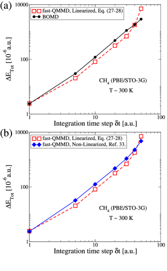
Figure 6: The local truncation error in a fast-QMMD calculation utilizing the linearized energy expression, Eq. (27), and force expression, Eq. (28), for vibrational motion of Methane for different time-steps. In (a) compared to the corresponding “exact” (5 SCF/step) Born-Oppenheimer molecular dynamics (BOMD) calculations, and in (b) compared to a fast-QMMD calculation using the corresponding “non-linearized” optimization-free energy and force expressions used in the previous study Souvatzis and Niklasson [2013]. Here the PBE functional PBE was used together with a STO-3G basis-set. All calculations were performed with a modified Verlet scheme (using $K$ = 7 in table 1 ) and a rescaling of $\kappa=\delta t^{2}\omega^{2}$ with a factor $\gamma$ = 0.7.

III.2 Finite electronic temperatures

Figure 3 illustrates the total energy conservation with ($E-T_{e}S$) and without ($E$) the electronic entropy contribution. At an electronic temperature of 10,000 K the fluctuations in total energy decrease by 1-2 orders of magnitude when the electronic entropy contribution is included. This high resolution could be critical in order to resolve small differences in the free energy between competing phases. Here it mainly illustrates that the constant of motion behaves as expected.

Because of the large HOMO-LUMO gap of the water system in Fig. 3, a fairly high temperature is needed to illustrate the electronic temperature effect. In Fig. 4 we show the corresponding finite temperature result for a small Lithium cluster (Li₅). In the restricted calculation of a system with an odd number of electrons, the highest occupied state has an occupation factor of $\sim 1/2$ and the entropy contribution is thus significant even at a fairly low electronic temperature ($T_{e}=1000$ K), as is seen in the upper panel (a). This example also illustrated the ability of the fast-QMMD scheme to simulate systems that may have significant problems to reach the self-consistent ground state. The lower panel shows the interatomic distance between two Li atoms. The fast-QMMD scheme provides molecular trajectories that are virtually on top of the Born-Oppenheimer result for over 4 ps of simulation time.

III.3 Translation, vibration, and rotation

It may appear that the fast-QMMD scheme is almost identical to an “exact” fully converged Born-Oppenheimer simulation. However, there is a subtle difference in the behavior of the local truncation error. Consider a pure translational motion of a molecular system. In this case there will be no transfer of energy from the kinetic to the potential energy. Given an atom centered basis set, the electronic ground state density matrix will remain constant and the local truncation error, i.e. the error in the ability to account for the correct energy transfer between kinetic and potential energy, will effectively be zero, both for a fast-QMMD and a Born-Oppenheimer simulation. This is not the case for a vibrational motion, where both fast-QMMD and Born-Oppenheimer simulations will have local truncation errors due to the finite integration time step and fail to exactly account for the balance in energy transfer between kinetic and potential energy. However, for rotational motion a difference appears between fast-QMMD and Born-Oppenheimer molecular dynamics simulations. As for a pure translational motion, a pure rotational mode has no energy transfer of kinetic energy. Nevertheless, since the matrix representation of the ground state density matrix change between time steps for a rotational motion, the fast-QMMD will show some small changes in the total energy due to the rotation, which will be absent in an “exact” Born-Oppenheimer simulation. Figure 5 illustrates this behavior. In the upper panel (a), which has a superposed vibrational and rotational motion, we find an additional oscillatory motion in the total energy of the fast-QMMD simulation compared to the Born-Oppenheimer simulation. This qualitative difference is not found in the lower panel (b), which only has a pure vibrational motion. For the general case of composite motion, we therefore expect fast-QMMD simulations to have a slightly increased local truncation error compared to an “exact” fully converged Born-Oppenheimer simulation.

III.4 Tunable accuracy

The sensitivity to the integration time step $\delta t$ could potentially be a limiting factor for the fast-QMMD scheme. Figure 6 (a) shows the local truncation error (measured by the amplitude of the oscillations of the total energy) as a function of the length of the time step $\delta t$ for fast-QMMD and Born-Oppenheimer simulations of a single Methane molecule at room temperature. The two curves both scale as $\sim\delta t^{2}$, where the fast-QMMD truncation errors are slightly smaller than the BOMD errors all the way up to $\delta t\approx 40$ a.u. (about 1 fs), where a small shift appears. Just as in a classical molecular dynamics simulation, the local truncation error is governed by the size of a tunable integration time step and not by the number of self-consistent field iterations. The general validity of this result is hard to judge, but the behavior in Fig. 6 (a) is consistent with what we have found so far in our simulations and can be expected to hold as long as there are no inherent self-consistent field instabilities or anomalous (non-convex) functional behavior.

III.5 Comparison to previous approach

In Fig. 6 (b) we show a comparison of the local truncation error as a function of the integration time step, $\delta t$, between our fast-QMMD using the linearized energy and force expression, Eqs. (25-31), and the corresponding fast-QMMD based on a “non-linearized” potential energy that was used in our previous Hartree-Fock simulations Souvatzis and Niklasson [2013]. Both methods require only one diagonalization per time step, but in contrast to the new linearized scheme, the previous method requires two full constructions of the effective Hamiltonian in each time step and the forces are approximate. The linearized version of the fast-QMMD scheme yields slightly smaller local truncation errors compared to the non-linearized version all the way up to a time-step, $\delta t\sim$ 40 a.u. ($\sim 1$ fs) above which the linearized formulation starts to diverge. We believe this improved behavior can be explained by the consistency between the forces and the potential energy for the linearized expression, which is valid as long as the linearization is sufficiently accurate, i.e. for $\delta t\lesssim$ 40 a.u. For normal simulations, with time steps of about 10-30 a.u., the stability and accuracy of the two approaches are comparable, but thanks to the lower complexity of the linearized approach, with only one Hamiltonian construction per time step, our new scheme represents a significant improvement.

III.6 Stability

The fast-QMMD scheme is robust to sudden perturbations. Figure 7 shows the total energy of a simulated water molecule. After about 2.4 ps of simulation time an abrupt significant change in the density matrix $D(P)$ is introduced. Despite this sudden large perturbation the energy relaxes and returns to a stable average value that is slightly shifted but close to the initial total energy. However, a fairly short integration temp step is required to account for the rapid change in density matrix. We believe this response to a sudden perturbation illustrates a key feature of the fast-QMMD scheme. Instead of optimizing the electronic structure in each individual time step prior to the force calculation, the electronic degrees of freedom is optimized dynamically as the trajectories propagate. The speed of the relaxation is slightly different for different choices of the scaling parameter $\gamma$. This difference indicates an interesting opportunity. It should be possible to dynamically update an optimal value of $\gamma$ in each time step. A time-dependent scaling factor, $\gamma(t)$, that is updated one-the-fly in a time-reversible way is an interesting opportunity for future developments.

Figure 7: Total energy of a fast-QMMD calculation of a single water molecule using the LDA density functional LDA . After $\sim$ 2400 fs the dynamics is perturbed by replacing the density matrix, $D$, with the initial density matrix, $D(t=0)$, calculated at the time, t = 0 s. The perturbation calculation was performed for three different $\kappa$-parameters (Eq. (31)). All calculations were performed with the modified Verlet integration ($K$ = 7 in table 1 ). Here rescaling of a $\kappa=\delta t^{2}\omega^{2}$ with a factor $\gamma$ = 0.7 was employed for the black curve, and $\gamma$ = 0.6 for the red curve.

IV Summary

The goal of this paper was to explore the extended Lagrangian formulation of Born-Oppenheimer molecular dynamics in the limit of vanishing self-consistent field optimization. In contrast to the most recent studies, Refs. Souvatzis and Niklasson [2013], we have generalized the first principles theory beyond the ground state Hartree-Fock method to include also free energy potential surfaces valid at finite electronic temperatures, density functional theory with hybrid functionals, as well as the requirement of only one single Hamiltonian construction per time step. This provides a very efficient and computational fast approach to first principles simulations that should be applicable to a broad class of materials. Under normal conditions the proposed fast-QMMD scheme yields trajectories that are practically indistinguishable from an ”exact” Born-Oppenheimer molecular dynamics simulation. However, even in the event of anomalous behavior that may cause numerical instabilities, the optimization-free limit represents an ideal framework for more elaborate force calculations that require an improved accuracy in the electronic ground state optimization or a reduced length of the integration time step to recover stability or to improve accuracy.

The optimization-free limit of extended Lagrangian Born-Oppenheimer molecular dynamics demonstrates some of the opportunities in the development of a new generation first principles molecular dynamics that avoids current problems and shortcomings and allows a wider range of applications. Our work presented in this article is a step in this direction.

V Acknowledgements

P. S. wants to thank L. C. for her eternal patience. A.M.N.N acknowledge support by the United States Department of Energy (U.S. DOE) Office of Basic Energy Sciences, discussions with M. Cawkwell, E. Chisolm, C.J. Tymczak, G. Zheng and stimulating contributions by T. Peery at the T-Division Ten Bar Java group. LANL is operated by Los Alamos National Security, LLC, for the NNSA of the U.S. DOE under Contract No. DE-AC52- 06NA25396. Support by the Göran Gustafsson research foundation is also gratefully acknowledged.

VI Appendix

VI.1 Forces without prior self-consistent field optimization

To derive the force expression in Eq. (18), which together with the energy expression in Eq. (15) is one of our key results, we start by noting that

$$\begin{array}[]{l}E^{xc}[2D]=E^{xc}[2P]+2Tr[(D-P)V^{xc}[2P]]\\ {}\\ +{\cal O}[(D-P)^{2}].\end{array}$$ (33)

Within the same order of accuracy, ${\cal O}((D-P)^{2})$, we can replace the expression in Eq. (15) by

$$\begin{array}[]{l}{\cal F}[P]=2Tr[hD]+Tr[(2D-P)G^{\alpha}(P)]\\ {}\\ +E^{xc}[2P]+2Tr[(D-P)V_{xc}[2P]]\\ {}\\ -T_{e}{\cal S}[D].\end{array}$$ (34)

Taking the partial derivative with respect to the nuclear coordinates (keeping $P$ constant) of the resulting free energy we get

$$\begin{array}[]{l}\left.\partial{\cal F}[P]/\partial R_{I}\right|_{P}={\cal F}_{R}=2Tr[h_{R}D+hD_{R}]\\ {}\\ ~{}+2Tr[D_{R}G^{\alpha}(P)]+Tr[(2D-P)G^{\alpha}_{R}(P)]\\ {}\\ ~{}+E^{xc}_{R}[2P]+2Tr[(D-P)V^{xc}_{R}(2P)]\\ {}\\ ~{}+2TR[D_{R}V^{xc}(2P)]-T_{e}\partial{\cal S}/\partial R_{I}\\ {}{}\\ =2Tr[h_{R}D]+Tr[(2D-P)G^{\alpha}_{R}(P)]\\ \\ ~{}+E^{xc}_{R}[2P]+2Tr[(D-P)V^{xc}_{R}(2P)]\\ {}\\ ~{}+2Tr[(h+G^{\alpha}(P)+V^{xc}(2P))D_{R}]-T_{e}{\cal S}_{R}\\ {}\\ =2Tr[h_{R}D]+Tr[(2D-P)G^{\alpha}_{R}(P)]\\ {}\\ ~{}+E^{xc}_{R}[2P]+2Tr[(D-P)V^{xc}_{R}(2P)]\\ {}\\ ~{}+2Tr[H(P)D_{R}]-T_{e}{\cal S}_{R}\\ \\ =2Tr[h_{R}D]+Tr[(2D-P)G^{\alpha}_{R}(P)]\\ {}\\ ~{}+E^{xc}_{R}[2D]+2Tr[H(P)D_{R}]-T_{e}{\cal S}_{R}\\ {}\\ ~{}+{\cal O}[(D-P)^{2}].\end{array}$$ (35)

In the last step we used a second order approximation of $E^{xc}_{R}[2D]$ expanded around $2P$, i.e. as in Eq. (33), where

$$\begin{array}[]{l}E^{xc}_{R}[2D]=E^{xc}_{R}[2P]+2Tr[(D-P)V^{xc}_{R}[2P]]\\ {}{}\\ +{\cal O}[(D-P)^{2}].\end{array}$$ (36)

Here the subscript $R$ in $V^{xc}_{R}(2P)$, $E^{xc}_{R}[2P]$, $E^{xc}_{R}[2D]$ and $G^{\alpha}_{R}(P)$ denotes a derivative with respect only to the underlying atom centered basis. We now need to simplify the last two terms of the derivative above. We start with

$$\begin{array}[]{l}2Tr[H(P)D_{R}]=2Tr[H(\partial D/\partial R)]\\ {}\\ =2Tr[H\partial(ZD^{\perp}Z^{T})/\partial R]\\ {}\\ =2Tr[H(Z_{R}D^{\perp}Z^{T}+ZD^{\perp}_{R}Z^{T}+ZD^{\perp}Z^{T}_{R})].\end{array}$$ (37)

By using the relation $Z_{R}=-(1/2)S^{-1}S_{R}Z$ proposed in Ref. Niklasson and Weber [2007] we get

$$\begin{array}[]{l}2Tr[H(P)D_{R}]=-Tr[HS^{-1}S_{R}D+HDS_{R}S^{-1}]\\ {}\\ ~{}+2Tr[H^{\perp}D^{\perp}_{R}]\\ {}\\ =-2Tr[S^{-1}HDS_{R}]+2Tr[H^{\perp}D^{\perp}_{R}],\\ \end{array}$$ (38)

where we in the first step used the cyclic invariance under the trace, and in the next step the commutation relation, $DH(P)S^{-1}-S^{-1}H(P)D=0$. The last term above, $2Tr[H^{\perp}D^{\perp}_{R}]$, vanish only for idempotent solutions at zero electronic temperatures. At finite temperatures, however, the $2Tr[H^{\perp}D^{\perp}_{R}]$ term is exactly cancelled by the entropy contribution, since

$$\begin{array}[]{l}{\displaystyle T_{e}{\cal S}_{R}=-2T_{e}k_{B}\frac{\partial}{\partial R}Tr\left[D^{\perp}\ln(D^{\perp})\right.}\\ {}\\ ~{}\left.+(I-D^{\perp})\ln(I-D^{\perp})\right]\\ {}\\ =-2\beta^{-1}Tr[D^{\perp}_{R}\ln(D^{\perp}/(I-D^{\perp})]\\ {}\\ =-2\beta^{-1}Tr[D^{\perp}_{R}\ln\left(e^{-\beta(H^{\perp}(P)-\mu I)}\right)]\\ {}\\ =2Tr[D^{\perp}_{R}H^{\perp}].\end{array}$$ (39)

In the last equation above we used the fact that $Tr[D^{\perp}_{R}]=0$, since we assume canonical, charge conserving, partial derivatives. Going back to the force derivation in Eq. (35) we now have that

$$\begin{array}[]{l}{\cal F}_{R}[P]=2Tr[h_{R}]+Tr[(2D-P)G^{\alpha}_{R}(P)]+E^{xc}_{R}[2D]\\ {}\\ ~{}-2Tr[S^{-1}HDS_{R}]+{\cal O}[(D-P)^{2}]\end{array}$$ (40)

which completes our derivation of Eq. (18).

References

- Marx and Hutter [2000] D. Marx and J. Hutter, Modern Methods and Algorithms of Quantum Chemistry (ed. J. Grotendorst, John von Neumann Institute for Computing, Jülich, Germany, 2000), 2nd ed.
- Kirchner [2012] B. Kirchner J. di Dio Philipp, and J. Hutter, Top. Curr. Chem. 307, 109 Springer Verlag, Berlin Heidelberg, (2012).
- Wang and Karplus [1973] I. S. Y. Wang and M. Karplus, J. Am. Chem. Soc. 95, 8160 (1973).
- Leforestier [1978] C. Leforestier, J. Chem. Phys. 68, 4406 (1978).
- Hohenberg and Kohn [1964] P. Hohenberg and W. Kohn, Phys. Rev. 136, B:864 (1964).
- Kohn and Sham [1965] W. Kohn and L. J. Sham, Phys. Rev. B 140, A1133 (1965).
- Cooley and Tukey [1965] J. W. Cooley and J. W. Tukey, Math. Comp. 19, 297 (1965).
- Car and Parrinello [1985] R. Car and M. Parrinello, Phys. Rev. Lett. 55, 2471 (1985).
- Remler and Madden [1990] D. K. Remler and P. A. Madden, Mol. Phys. 70, 921 (1990).
- Vanderbilt [1990] D. Vanderbilt, Phys. Rev. B 41, 7892 (1990).
- Payne et al. [1992] M. C. Payne, M. P. Teter, D. C. Allan, T. A. Arias, and J. D. Joannopoulos, Rev. Mod. Phys. 64, 1045 (1992).
- Kresse [1993] G. Kresse, and J. Hafner, Phys. Rev. B 47, 558 (1993).
- Barnett [1993] R. N. Barnett, and U. Landman, Phys. Rev. B 48, 2081 (1993).
- Pulay and Fogarasi [2004] P. Pulay and G. Fogarasi, Chem. Phys. Lett. 386, 272 (2004).
- Hartke [1992] B. Hartke, and E. A. Carter, Chem. Phys. Lett. 189, 358 (1992).
- Tuckerman [2002] M. Tuckerman, J. Phys.:Condens. Matter 50, 1297 (2002).
- Schlegel [2001] H. B. Schlegel, J. M. Millam, S. S. Iyengar, G. A. Voth, A. D. Daniels, G. Scusseria, and M. J. Frisch, J. Chem. Phys. 114, 9758 (2001).
- Herbert [1992] J. Herbert, and M. Head-Gordon, J. Chem. Phys. 121, 11542 (2004).
- Schlegel [2002] H. B. Schlegel, S. Srinivasan, S. S. Iyengar, X. Li, J. M. Millam, G. A. Voth, G. Scusseria, and M. J. Frisch, J. Chem. Phys. 117, 8694 (2002).
- Arias et al. [1992] T. Arias, M. Payne, and J. Joannopoulos, Phys. Rev. Lett. 69, 1077 (1992).
- Niklasson et al. [2006] A. M. N. Niklasson, C. J. Tymczak, and M. Challacombe, Phys. Rev. Lett. 97, 123001 (2006).
- Kühne et al. [2006] T. D. Kühne, M. Krack, F. R. Mohamed, and M. Parrinello, Phys. Rev. Lett. 98, 066401 (2006).
- Alonso [2008] J. L. Alonso, X. Andrade, P. Echenique, F. Falceto, D. Prada-Garcia, A. Rubio, Phys. Rev. Lett. 101, 096403 (2008).
- Jakowski [2009] J. Jakowski, and K. Morokuma, J. Chem. Phys. 130, 224106 (2009).
- Hutter [2012] J. Hutter, WIREs Comput. Mol. Sci. 2, 604 (2012).
- Niklasson [2008] A. M. N. Niklasson, Phys. Rev. Lett. 100, 123004 (2008).
- Zheng et al. [2011] G. Zheng, A. M. N. Niklasson, and M. Karplus, J. Chem. Phys. 135, 044122 (2011).
- Steneteg et al. [2010] P. Steneteg, I. A. Abrikosov, V. Weber, and A. M. N. Niklasson, Phys. Rev. B 82, 075110 (2010).
- Lin et al. [2013] L. Lin, J. Lu, and S. Shao, Entropy 16, 110 (2014). (http://arxiv.org/abs/1306.3016)
- Niklasson et al. [2011] A. M. N. Niklasson, P. Steneteg, and N. Bock, J. Chem. Phys. 135, 164111 (2011).
- Cawkwell and Niklasson [2012] M. J. Cawkwell, and A. M. N. Niklasson, J. Chem. Phys. 137, 134105 (2012).
- Niklasson and Cawkwell [2012] A. M. N. Niklasson, and M. J. Cawkwell, Phys. Rev. B 86, 174308 (2012).
- Souvatzis and Niklasson [2013] P. Souvatzis, and A. M. N. Niklasson, J. Chem. Phys. 139, 214102 (2013).
- Niklasson et al. [2009] A. M. N. Niklasson, P. Steneteg, A. Odell, N. Bock, M. Challacombe, C. J. Tymczak, E. Holmström, G. Zheng, and V. Weber, J. Chem. Phys. 130, 214109 (2009).
- McWeeny [1960] R. McWeeny, Rev. Mod. Phys. 32, 335 (1960).
- Roothaan [1951] C. C. J. Roothaan, Rev. Mod. Phys. 23, 69 (1951).
- Parr and Yang [1989] R. G. Parr and W. Yang, Density-functional theory of atoms and molecules (Oxford University Press, Oxford, 1989).
- Dreizler and Gross [1990] R. M. Dreizler and K. U. Gross, Density-functional theory (Springer Verlag, Berlin Heidelberg, 1990).
- Pulay [1969] P. Pulay, Mol. Phys. 17, 197 (1969).
- Feynman [1939] R. P. Feynman, Phys. Rev. 56, 367 (1939).
- Odell et al. [2009] A. Odell, A. Delin, B. Johansson, N. Bock, M. Challacombe, and A. M. N. Niklasson, J. Chem. Phys. 131, 244106 (2009).
- Odell et al. [2011] A. Odell, A. Delin, B. Johansson, M. Cawkwell, and A. M. N. Niklasson, J. Chem. Phys. 135, 224105 (2011).
- [43] Y. Zhang, W. Yang, Phys. Rev. Lett. 80 (1998) 890.
- [44] S. Vosko, L. Wilk, M. Nusair, Canad. J. Phys. 58 (1980) 1200.
- [45] P. J. Stephens, F. J. Devlin, C. F. Chabalowski, and M. J. Frisch, J. Phys. Chem. 98, 11623 (1994).
- Weinert and Davenport [1992] M. Weinert and J. W. Davenport, Phys. Rev. B 45, R13709 (1992).
- Wentzcovitch et al. [1992] R. M. Wentzcovitch, J. L. Martins, and P. B. Allen, Phys. Rev. B 45, R11372 (1992).
- Niklasson [2008b] A. M. N. Niklasson, J. Chem. Phys. 129, 244107 (2008b).
- UQuantChem [2013] P. Souvatzis, Comp. Phys. Comm. 185, 415-421 (2014).
- UQuantChem [2010] The UQuantChem code written by P. Souvatzis can be obtained from, http://www.anst.uu.se/pesou087/ UU-SITE/Webbplats_2/UQUANTCHEM.html or from https://github.com/petrossou/uquantchem
- Niklasson and Weber [2007] A. M. N. Niklasson, and W. Weber, J. Chem. Phys. 127, 064105 (2007).