Stellar Diameters and Temperatures V.
Eleven Newly Characterized Exoplanet Host Stars

Abstract

We use near-infrared interferometric data coupled with trigonometric parallax values and spectral energy distribution fitting to directly determine stellar radii, effective temperatures, and luminosities for the exoplanet host stars 61 Vir, $\rho$ CrB, GJ 176, GJ 614, GJ 649, GJ 876, HD 1461, HD 7924, HD 33564, HD 107383, and HD 210702. Three of these targets are M dwarfs. Statistical uncertainties in the stellar radii and effective temperatures range from 0.5% – 5% and from 0.2% – 2%, respectively. For eight of these targets, this work presents the first directly determined values of radius and temperature; for the other three, we provide updates to their properties. The stellar fundamental parameters are used to estimate stellar mass and calculate the location and extent of each system’s circumstellar habitable zone. Two of these systems have planets that spend at least parts of their respective orbits in the system habitable zone: two of GJ 876’s four planets and the planet that orbits HD 33564. We find that our value for GJ 876’s stellar radius is more than 20% larger than previous estimates and frequently used values in the astronomical literature.

1 Introduction

In the characterization of exoplanetary systems, knowledge of particularly the stellar radius and temperature are of paramount importance as they define the radiation environment in which the planets reside, and they enable the calculation of the circumstellar habitable zone’s (HZ) location and boundaries. Furthermore, the radii and densities of any transiting exoplanets, which provide the deepest insights into planet properties such as exoatmospheric studies or the studies of planetary interior structures, are direct functions of the radius and mass of the respective parent star. Recent advances in sensitivity and angular resolution in long-baseline interferometry at wavelengths in the near-infrared and optical range have made it possible to circumvent assumptions of stellar radius by enabling direct measurements of stellar radius and other astrophysical properties for nearby, bright stars (e.g., Baines et al., 2008b, a, 2009, 2010; van Belle & von Braun, 2009; von Braun et al., 2011a, b, 2012; Boyajian et al., 2012a, b, 2013; Huber et al., 2012, and references therein).

In this paper, we present interferometric observations (§2.1) that, in combination with trigonometric parallax values, produce directly determined stellar radii for eleven exoplanet host stars, along with estimates of their stellar effective temperatures based on literature photometry (§3). We use these empirical stellar parameters to calculate stellar masses/ages where possible, and the locations and boundaries of the system HZs (§3.2). We discuss the implications for all the individual systems in §4 and conclude in §5.

2 Data

In order to be as empirical as possible in the calculation of the stellar parameters of our targets, we rely on our interferometric observations to obtain angular diameters (§2.1), and we fit empirical spectral templates to literature photometry to obtain bolometric flux values (§2.2).

2.1 Interferometric Observations

Our observational methods and strategy are described in detail in §2.1 of Boyajian et al. (2013). We repeat aspects specific to the observations of the individual targets below.

The Georgia State University Center for High Angular Resolution Astronomy (CHARA) Array (ten Brummelaar et al., 2005) was used to collect our interferometric observations of exoplanet hosts in $J,H$, and $K^{\prime}$ bands with the CHARA Classic beam combiner in single-baseline mode. The data were taken between 2010 and 2013 in parallel with our interferometric survey of main-sequence stars (Boyajian et al., 2012b, 2013). Our requirement that any target be observed on at least two nights with at least two different baselines serves to eliminate or reduce systematic effects in the observational results (von Braun et al., 2012; Boyajian et al., 2013). We note that were not able to adhere this strategy for HD 107383, which was only observed during one night due to weather constraints during the observing run.

An additional measure to reduce the influence of systematics is the alternating between multiple interferometric calibrators during observations to eliminate effects of atmospheric and instrumental systematics. Calibrators, whose angular sizes are estimated using size estimates from the Jean-Marie Mariotti Center JMDC Catalog at http://www.jmmc.fr/searchcal (Bonneau et al., 2006, 2011; Lafrasse et al., 2010b, a), are chosen to be small sources of similar brightness as, and small angular distance to, the respective target. A log of the interferometric observations can be found in Table 1.

The uniform disk and limb-darkened angular diameters ($\theta_{\rm UD}$ and $\theta_{\rm LD}$, respectively; see Table 2) are found by fitting the calibrated visibility measurements (Fig. 1 and 2) to the respective functions for each relation. These functions may be described as $n^{th}$-order Bessel functions that are dependent on the angular diameter of the star, the projected distance between the two telescopes and the wavelength of observation (Hanbury Brown et al., 1974). The temperature-dependent limb-darkening coefficients, $\mu_{\lambda}$, used to convert from $\theta_{\rm UD}$ to $\theta_{\rm LD}$, are taken from Claret (2000) after we iterate based on the effective temperature value obtained from initial spectral energy distribution fitting (see §2.2). Limb-darkening coefficients are dependent on assumed stellar effective temperature, surface gravity, and weakly on metallicity. When we vary the input $T_{\rm eff}$ by 200 K and $\log g$ by 0.5 dex, the resulting variations are below 0.1% in $\theta_{\rm LD}$ and below 0.05% in $T_{\rm eff}$. Varying the assumed metallicity across the range of our target sample does not influence our final values of $\theta_{\rm LD}$ and $T_{\rm eff}$ at all.

The values for $\theta_{\rm UD}$ and $\theta_{\rm LD}$ for our targets are given in Table 2. The angular diameters and their respective uncertainties are computed using MPFIT, a non-linear least-squares fitting routine in IDL (Markwardt, 2009). Table 2 shows the empirical $\chi^{2}_{reduced}$ values of the fits shown in Figures 1 and 2 in column 3. These $\chi^{2}_{reduced}$ values are often calculated to be $<<1$ due to the difficulty of accurately defining uncertainties in the visibility measurements. Consequently, we assume a true $\chi^{2}_{reduced}$ = 1 when calculating the uncertainties for $\theta_{\rm UD}$ and $\theta_{\rm LD}$, based on a rescaling of the associated uncertainties in the visibility data points. That is, the estimates of our uncertainties in $\theta_{\rm UD}$ and $\theta_{\rm LD}$ are based on a $\chi^{2}_{reduced}$ fit, not on strictly analytical calculations.

Figure 1: Plots of calibrated interferometric visibilities and fits. The separated cluster of data points shown as open circles in the visibility fit for GJ 614 with a relatively large spread in visibility that is located at smaller spatial frequencies (lower numeric values in baseline / wavelength) is comprised of literature $K^{\prime}$ data from Baines et al. (2008b) – see §4.4 for details. The interferometric observations are described in §2.1.

Figure 2: Plots of calibrated interferometric visibilities and fits. See §2.1 for details on the interferometric observations.

Table 1: Log of Interferometric Observations

Star		# of
UT Date	Baseline	Obs (filter)	Calibrators
61 Vir
2012/04/09	W1/E1	13($H$)	HD 113289, HD 116928
2012/04/10	S1/E1	3($H$)	HD 113289, HD 116928
$\rho$ CrB
2013/05/03	S1/E1	4($H$)2($K^{\prime}$)	HD 139389, HD 149890
2013/08/18	S1/W1	3($H$)	HD 139389, HD 146946
GJ 176
2010/09/16	W1/E1	7($H$)	HD 29225, HD 27524
2010/09/17	W1/E1	2($H$)	HD 27534
2010/09/20	S1/E1	4($H$)	HD 29225
2010/11/10	W1/E1	3($H$)	HD 29225
GJ 614
2010/06/28	W1/E1	10($H$)	HD 144579, HD 142908
2010/06/29	W1/E1	6($H$)	HD 144579, HD 142908
2010/09/18	S1/E1	4($H$)	HD 144579
GJ 649
2010/06/29	W1/E1	5($H$)	HD 153897
2010/06/30	S1/E1	6($H$)	HD 153897, HD150205
2010/07/01	S1/E1	7($H$)	HD 153897, HD150205
GJ 876
2011/08/17	S1/E1	11($H$)	HD 215874, HD 217681
2011/08/18	S1/E1	10($H$)	HD 215874, HD 217681
2011/08/19	W1/E1	6($H$)	HD 215874, HD 216402
2011/08/20	W1/E1	6($H$)	HD 217861, HD 216402
HD 1461
2011/08/22	S1/E1	7($H$)	HD 966, HD 1100
2011/10/03	S1/E1	7($H$)	HD 966, HD 1100
2013/08/17	E1/W1	5($H$)	HD 966, HD 1100
HD 7924
2010/09/17	W1/E1	9($H$)	HD 9407, HD 6798
2011/08/21	W1/S1	6($H$)	HD 9407, HD 6798
HD 33564
2010/09/16	W1/E1	2($H$)	HD 29329
2010/09/17	W1/E1	1($H$)	HD 62613
2010/11/10	W1/E1	9($H$)	HD 36768, HD 46588
2013/08/16	S1/W1	3($H$)	HD 29329, HD 62613
2013/08/17	S1/W1	1($H$)	HD 29329, HD 36768, HD 46588
HD 107383
2013/05/06	E2/W2	3($H$)	HD 106661, HD 108468
2013/05/06	S2/W2	4($H$)	HD 106661, HD 104452
HD 210702
2013/08/18	S1/E1	5($H$)1($J$)	HD 210074, HD 206043
2013/08/19	E1/W1	2($H$)	HD 210074, HD 206043
2013/08/22	E1/W1	7($H$)	HD 210074, HD 207223
2013/08/22	S1/E1	1($J$)	HD 210074, HD 207223

Table 2: Stellar Angular Diameters

Star	# of	Reduced	$\theta_{\rm UD}\pm\sigma$		$\theta_{\rm LD}\pm\sigma$	$\theta_{\rm LD}$
Name	Obs.	$\chi^{2}$	(mas)	$\mu_{\lambda}$	(mas)	% err
61 Vir	16	0.31	$1.037\pm 0.005$	0.367	$1.073\pm 0.005$	0.4
$\rho$ CrB	9	0.46	$0.714\pm 0.013$	0.342	$0.735\pm 0.014$	1.9
GJ 176	14	0.18	$0.441\pm 0.020$	0.210	$0.448\pm 0.021$	4.6
GJ 614	28	1.16	$0.449\pm 0.017$	0.284	$0.459\pm 0.017$	3.7
GJ 649	18	1.02	$0.472\pm 0.012$	0.327	$0.484\pm 0.012$	2.5
GJ 876	33	0.32	$0.721\pm 0.009$	0.398	$0.746\pm 0.009$	1.2
HD 1461	16	0.19	$0.483\pm 0.010$	0.369	$0.498\pm 0.011$	2.1
HD 7924	15	0.19	$0.424\pm 0.014$	0.281	$0.433\pm 0.014$	3.2
HD 33564	16	1.08	$0.629\pm 0.010$	0.225	$0.640\pm 0.010$	1.6
HD 107383	7	0.16	$1.590\pm 0.015$	0.417	$1.651\pm 0.016$	1.0
HD 210702	16	1.57	$0.845\pm 0.005$	0.484	$0.886\pm 0.006$	0.6

2.2 Bolometric Fluxes

In this Section, we report on stellar spectral energy distributions (SEDs) fits of our targets. We augment literature broad-band photometry data by using spectrophotometric data whenever available. The purpose of these SED fits is to obtain direct estimates of stellar $T_{\rm eff}$ and $L$, as described in §3.1. Our procedure is analogous to the ones performed in van Belle & von Braun (2009); von Braun et al. (2011a, b, 2012); Boyajian et al. (2012a, b, 2013).

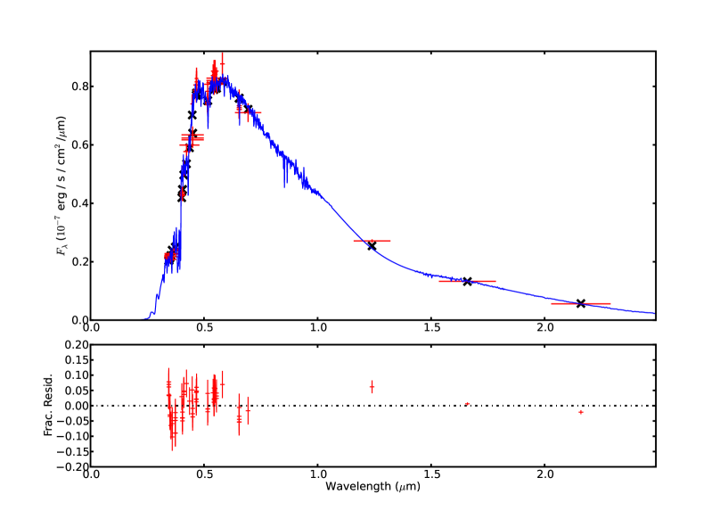
Figure 3: SED Fit of GJ 614 to illustrate our fitting routine. In the top panel, the (blue) spectrum is a G9 IV spectral template from the Pickles (1998) library. The (red) crosses indicate photometry values from the literature. “Error bars” in x-direction represent the bandwidths of the photometric filters. The (black) X-shaped symbols indicate the flux value of the spectral template averaged over the filter transmission range in wavelength. The lower panel shows the residuals around the fit in fractional flux units of photometric uncertainty. The uncertainties in y-direction in the lower plot represent the photometric uncertainties in the literature data scaled by the corresponding flux values. For more details, see §2.2.

Our SED fitting is based on a $\chi^{2}$-minimization of input SED templates from the Pickles (1998) to literature photometry of the star under investigation. If the literature photometry values are in magnitudes, they are converted to absolute fluxes by application of published or calculated zero points. The filters of the literature photometry data are assumed to have a top-hat shape. That is, during the calculation of $\chi^{2}$, only the central filter wavelengths are correlated with the SED template’s flux value averaged over the filter transmission range in wavelength. Literature spectrophometry data are very useful for SED fitting since multiple individual photometry data points, instead of being integrated into a single wavelength, trace out the shape of the SED in great detail. The SED template is scaled to minimize $\chi^{2}$ and then integrated over wavelength to obtain the bolometric flux. The code additionally produces an estimated angular diameter, which we only use as a sanity check to avoid systematic problems like the choice of wrong spectral template. Figure 3 illustrates our procedure for the example of GJ 614.

We note that our quoted uncertainties on the bolometric flux values are statistical only. We do not (and indeed cannot) account for possible systematics such as saturation or correlated errors in the photometry, filter errors due to problems with transmission curves, or other non-random error sources. The only systematics that we can control are (1) the choice of spectral template for the SED fit, (2) the choice of which photometry data to include in the fit, and (3) whether to let the interstellar reddening float during the fit or whether to set it to zero. In order to be consistent as possible, we take the following approach:

• All photometry data are included in the fit in principle, except when they present clear outliers in the SED. This way, we attempt to reduce systematics. In general, there are tens to hundreds of photometric measurements per target (see Table 3), and at most, we remove 1–2 data points, mostly in the $U$ band or $RI$ bands.

• Interstellar extinction is set to zero for all targets, due to the small distances to the stars (see Table 4), which are adopted from van Leeuwen (2007). We cross-checked results with the ones using variable reddening, and in almost no case was there any difference. The ones for which the variable reddening produced results that are not consistent with $A_{V}=0$ at the $\sim$1-$\sigma$ level are discussed below. For all others, letting $A_{V}$ vary produced $A_{V}=0$.

• Whenever a literature photometry datum has no quoted uncertainty associated with it, we assign it a 5% random uncertainty. This is only the case for some older data sets.

• The choice of spectral template is based on minimization of $\chi_{reduced}^{2}$ only. For about half of our targets, we linearly interpolate between the relatively coarse grid of the Pickles (1998) spectral templates to obtain a better fit and thus a more accurate value for the numerical integration to calculate the bolometric flux (indicated in Table 3). Linear interpolation never spans more than three tenths in spectral type range (e.g., G5 to G8).

• Despite the fact that spectrophotometry often increases the fit’s $\chi_{reduced}^{2}$, we include these data whenever available (indicated in Table 3) in order to reduce the systematics in the choice of spectral template, which is determined more accurately via spectrophotometry.

Notes on individual systems with respect to SED fitting:

• 61 Vir: Despite the fact that we find $A_{V}=0$ when letting $A_{V}$ float, we note that dust excess for this system was reported in Trilling et al. (2008); Tanner et al. (2009); Bryden et al. (2009); Lawler et al. (2009). Photometry sources: Johnson et al. (1966); Johnson & Mitchell (1975); Golay (1972); Dean (1981); Haggkvist & Oja (1987); Olsen (1994); Oja (1996); spectrophotometry from Burnashev (1985).

• $\rho$ CrB: Photometry sources: Argue (1963); Golay (1972); Clark & McClure (1979); Haggkvist & Oja (1987); Beichman et al. (1988); Jasevicius et al. (1990); Kornilov et al. (1991); Skiff (1994); Glushneva et al. (1998); Gezari et al. (1999); Cutri et al. (2003); spectrophotometry from Burnashev (1985).

• GJ 176: Photometry sources: Weis (1984); Stauffer & Hartmann (1986); Weis (1986, 1987, 1993, 1996); Gezari et al. (1999); Bessell (2000); Cutri et al. (2003).

• GJ 614: Photometry sources: Argue (1963); Golay (1972); Beichman et al. (1988); Kornilov et al. (1991); Cutri et al. (2003); Kazlauskas et al. (2005).

• GJ 649: Photometry sources: Mumford (1956); Jones et al. (1981); Mermilliod (1986); Stauffer & Hartmann (1986); Beichman et al. (1988); Weis (1993, 1996); Cutri et al. (2003); Kazlauskas et al. (2005).

• GJ 876: With a variable $A_{V}$, the SED fit for GJ 876 produces slightly different results compared to the ones given in Table 3, where it was set to zero: $\chi^{2}_{red}$ = 4.86, $F_{\rm BOL}=(1.95\pm 0.001)\times 10^{-8}$ erg $\rm s^{-1}\rm cm^{-2}$ with an $A_{V}=0.111\pm 0.007$. Photometry sources: Erro (1971); Iriarte (1971); Golay (1972); Mould & Hyland (1976); Persson et al. (1977); Jones et al. (1981); Weis & Upgren (1982); The et al. (1984); Kozok (1985); Weis (1986, 1987); Bessel (1990); Weis (1996); Bessell (2000); Koen et al. (2002); Cutri et al. (2003); Kilkenny et al. (2007); Koen et al. (2010).

• HD 1461: Photometry sources: Cousins & Stoy (1962); Golay (1972); Sperauskas et al. (1981); Haggkvist & Oja (1987); Kornilov et al. (1991); Cutri et al. (2003); Kazlauskas et al. (2005).

• HD 7924: Photometry sources: Sanders (1966); Golay (1972); Kornilov et al. (1991); Cutri et al. (2003).

• HD 33564: With a variable $A_{V}$, the SED fit for HD 33564 produces slightly different results compared to the ones given in Table 3: $\chi^{2}_{red}$ = 3.81, $F_{\rm BOL}=(25.05\pm 0.19)\times 10^{-8}$ erg $\rm s^{-1}\rm cm^{-2}$ with an $A_{V}=0.076\pm 0.007$. Photometry sources: Häggkvist & Oja (1966); Golay (1972); Beichman et al. (1988); Cernis et al. (1989); Gezari et al. (1999); Kornilov et al. (1991); Cutri et al. (2003); spectrophotometry from Kharitonov et al. (1988).

• HD 107383: Photometry sources: Johnson et al. (1966); Häggkvist & Oja (1970); Straizys (1970); Golay (1972); Johnson & Mitchell (1975); Beichman et al. (1988); Kornilov et al. (1991); Yoss & Griffin (1997); Cutri et al. (2003).

• HD 210702: With a variable $A_{V}$, the SED fit for HD 210702 produces marginally different results compared to the ones given in Table 3: $\chi^{2}_{red}$ = 0.77, $F_{\rm BOL}=(14.24\pm 0.05)\times 10^{-8}$ erg $\rm s^{-1}\rm cm^{-2}$ with an $A_{V}=0.037\pm 0.029$. Photometry sources: Johnson & Knuckles (1957); Johnson et al. (1966); Golay (1972); Olson (1974); McClure & Forrester (1981); Kornilov et al. (1991); Cutri et al. (2003).

Table 3: $F_{\rm BOL}$ Values from SED Fitting

	Template	Degrees of		$F_{\rm BOL}\pm\sigma$
Star	Sp. Type	Freedom	$\chi^{2}_{red}$	($10^{-8}$ erg $\rm s^{-1}\rm cm^{-2}$)
61 Vir	G6.5V	233	2.81	36.06 $\pm$ 0.05
$\rho$ CrB	G0V	369	8.74	18.03 $\pm$ 0.02
GJ 176	M2.5V	36	5.95	1.26 $\pm$ 0.005
GJ 614	G9IV	69	1.28	6.50 $\pm$ 0.02
GJ 649	M2V	32	8.90	1.30 $\pm$ 0.005
GJ 876	M3.5V	109	7.18	1.78 $\pm$ 0.004
HD 1461	G2IV	91	0.63	6.95 $\pm$ 0.03
HD 7924	K0.5V	16	2.37	4.14 $\pm$ 0.03
HD 33564	F6V	119	4.88	23.17 $\pm$ 0.04
HD 107383	K0.5III	68	1.60	44.49 $\pm$ 0.25
HD 210702	G9III	47	0.79	13.65 $\pm$ 0.09

3 Stellar Astrophysical Parameters

In this Section, we report on our direct measurements of stellar diameters, $T_{\rm eff}$, and luminosities, based on our interferometric measurements (§2.1) and SED fitting to literature photometry (§2.2). We furthermore present calculated values wherever sensible for our targets, such as the location and extent of the respective system’s circumstellar habitable zone (HZ) and stellar mass and age. Results are summarized in Table 4.

3.1 Direct: Stellar Radii, Effective Temperatures, and Luminosities

We use our measured, limb-darkening corrected, angular diameters $\theta_{\rm LD}$, corresponding to the angular diameter of the Rosseland, or mean, radiating surface of the star (§2.1, Table 2), coupled with trigonometric parallax values from van Leeuwen (2007) to determine the linear stellar diameters. Uncertainties in the physical stellar radii are typically dominated by the uncertainties in the angular diameters, not the distance.

From the SED fitting (§2.2, Table 3), we calculate the value of the stellar bolometric flux, $F_{\rm BOL}$ by numerically integration of the scaled spectral template across all wavelengths. Wherever the empirical spectral template does not contain any data, it is interpolated and extrapolated along a blackbody curve. Combination with the rewritten version of the Stefan-Boltzmann Law

$$T_{\rm eff}({\rm K})=2341(F_{\rm BOL}/\theta_{\rm LD}^{2})^{\frac{1}{4}},$$ (1)

where $F_{\rm BOL}$ is in units of $10^{-8}$ erg cm^-2 s^-1 and $\theta_{\rm LD}$ is in units of mas, produces the effective stellar temperatures $T_{\rm eff}$.

3.2 Calculated: Habitable Zones, Stellar Masses and Ages

To first order, the habitable zone of a planetary system is described as the range of distances in which a planet with a surface and an atmosphere containing a modest amount of greenhouse gases would be able to host liquid water on its surface, first characterized in Kasting et al. (1993). The HZ boundaries in this paper are calculated based on the updated formalism of Kopparapu et al. (2013a, b). Kopparapu et al. (2013b) define the boundaries based on a runaway greenhouse effect or a runaway snowball effect as a function of stellar luminosity and effective temperature, plus water absorption by the planetary atmosphere. Whichever assumption is made of how long Venus and Mars were able to retain liquid water on their respective surfaces defines the choice of HZ (conservative or optimistic). These conditions are described in more detail in Kopparapu et al. (2013b) and section 3 of Kane et al. (2013). The boundaries quoted in Table 4 are the ones for both the conservative and optimistic HZ.

For stellar mass and age estimates of the early stars in our sample, we use the Yonsei-Yale ($Y^{2}$) isochrones (Yi et al., 2001; Kim et al., 2002; Demarque et al., 2004). Input data are our directly determined stellar radii and temperatures, along with the literature metallicity values from Table 4, and zero $\alpha$-element enhancement: [$\alpha$/Fe] $=0$. We follow the arguments in section 2.4 in Boyajian et al. (2013) and conservatively estimate mass and age uncertainties of 5% and 5 Gyr, respectively.

The ages of low-mass stars, however, are not sensitive to model isochrone fitting. Thus, in order to estimate the stellar masses of the KM dwarfs in our sample, we use the formalism described in §5.4 in Boyajian et al. (2012b). We use the data from Table 6 in Boyajian et al. (2012b) to derive the following equation for KM dwarfs:

$$M = -0.0460(\pm 0.0251)+1.0930(\pm 0.1481)R+$$ (2)

$$0.0064(\pm 0.1722)R^{2},$$

where $R$ and $M$ are the stellar radius and mass in Solar units, respectively. This essentially represents the inverted form of equation 10 in Boyajian et al. (2012b) for single dwarf stars. We note that the statistical errors in the determined masses using Equation 2 are dominated by the uncertainties in the coefficients and are of order $\sim 30$%.

Table 4: Stellar Astrophysical Parameters

	Radius	$T_{\rm eff}$	$L$	Spectral	Distance	Metallicity	$\rm HZ_{cons}$	$\rm HZ_{opt}$	Age	Mass
Star	($R_{\odot}$ )	(K)	($L_{\odot}$ )	Type	(pc)	[Fe/H]	(AU)	(AU)	(Gyr)	($M_{\odot}$)
61 Vir	$0.9867\pm 0.0048$	$5538\pm 13$	$0.8222\pm 0.0033$	G7 V	8.56	0.01	0.91 – 1.56	0.69 – 1.63	8.6	0.93
$\rho$ CrB	$1.3617\pm 0.0262$	$5627\pm 54$	$1.7059\pm 0.0423$	G0 V	17.43	-0.22	1.30 – 2.23	0.98 – 2.33	12.9	0.91
GJ 176	$0.4525\pm 0.0221$	$3679\pm 77$	$0.0337\pm 0.0018$	M2	9.27	0.15	0.20 – 0.37	0.15 – 0.38	–	0.45
GJ 614	$0.8668\pm 0.0324$	$5518\pm 102$	$0.6256\pm 0.0077$	K0 IV-V	15.57	0.44	0.79 – 1.37	0.60 – 1.43	–	0.91
GJ 649	$0.5387\pm 0.0157$	$3590\pm 45$	$0.0432\pm 0.0013$	M0.5	10.34	-0.04	0.22 – 0.42	0.17 – 0.44	–	0.54
GJ 876	$0.3761\pm 0.0059$	$3129\pm 19$	$0.0122\pm 0.0002$	M4	4.69	0.19	0.12 – 0.23	0.09 – 0.24	–	0.37
HD 1461	$1.2441\pm 0.0305$	$5386\pm 60$	$1.1893\pm 0.0476$	G3 V	23.44	0.16	1.10 – 1.89	0.83 – 1.98	13.8	0.94
HD 7924	$0.7821\pm 0.0258$	$5075\pm 83$	$0.3648\pm 0.0077$	K0 V	16.82	-0.14	0.62 – 1.08	0.47 – 1.13	–	0.81
HD 33564	$1.4367\pm 0.0238$	$6420\pm 50$	$3.1777\pm 0.0696$	F7 V	20.98	0.08	1.73 – 2.88	1.31 – 3.00	2.2	1.31
HD 107383	$15.781\pm 0.3444$	$4705\pm 24$	$109.51\pm 4.3256$	K0 III	88.89	-0.30	10.8 – 19.4	8.19 – 20.3	–	–
HD 210702	$5.2314\pm 0.1171$	$4780\pm 18$	$12.838\pm 0.5569$	K1 III	54.95	0.03	3.70 – 6.59	2.80 – 6.90	5.0	1.29

4 Discussion

In this Section, we briefly discuss our results on the individual systems. We compare our directly determined stellar parameters (§3.1 and Table 4) to quoted literature values. Statistical differences between values are calculated by adding our uncertainties and those from the literature, when available, in quadrature.

4.1 61 Vir (= HD 115617)

61 Vir hosts three planets with periods ranging from 4.2 to 124 days and minimum masses between 5.1 and 24 $M_{\earth}$ (Vogt et al., 2010). Since the orbital distances of all three planets are less than 0.5 AU from the parent star, and since the inner edge of the optimistic/conservative HZ is located at 0.69 AU / 0.91 AU, none of the known three planets reside within the system’s HZ.

The stellar radius for 61 Vir quoted in Takeda et al. (2007, $0.98\pm 0.03R_{\odot}$) is statistically identical with ours. When compared to Valenti & Fischer (2005), our radius measurement is $\sim 2\sigma$ larger than their estimate ($0.963\pm 0.011R_{\odot}$), while our temperature value is consistent with their value ($5571\pm 44$ K). Similarly good agreement exists with the $T_{\rm eff}$ value quoted in Ecuvillon et al. (2006, $5577\pm 33$ K).

To estimate 61 Vir’s mass and age, we use the $Y^{2}$ isochrones with our values from Table 4 as input, generated with a $0.1$ Gyr step size, and a fixed metallicity of [Fe/H] $=+0.01$ (Table 4). Interpolation within the best fitting isochrone gives an age of $8.6$ Gyr and mass of $0.93M_{\odot}$.

4.2 $\rho$ CrB (= HD 143761)

$\rho$ CrB has a Jupiter-mass planet in a 40-day orbit (Noyes et al., 1997) whose orbital semi-major axis (0.22 AU; Butler et al., 2006) is located well inside the system’s optimistic/conservative HZ’s inner boundary at 0.98 AU / 1.3 AU.

$\rho$ CrB’s radius was interferometrically observed in $K^{\prime}$-band by Baines et al. (2008b) who calculate a radius of $1.284\pm 0.082R_{\odot}$, well within $1\sigma$ of our value of $1.3424R_{\odot}$. $\rho$ CrB’s stellar radius from Fuhrmann et al. (1998), $1.34\pm 0.05R_{\odot}$, also agrees very well ($<<1\sigma$) with our directly determined value. The spectroscopically determined $T_{\rm eff}$ values of Fuhrmann et al. (1998, $5821\pm 80$ K) and Valenti & Fischer (2005, $5822\pm 44$ K), however, come in at $1.8\sigma$ and $2.7\sigma$ above our estimate of 5665 K.

Using the same procedure as for 61 Vir (§4.1), we solve for best-fit $Y^{2}$ isochrone properties for $\rho$ CrB using a metallicity of [Fe/H] $=-0.22$ (Table 4). This produces estimates for stellar age of 12.9 Gyr and stellar mass of $0.91M_{\odot}$.

4.3 GJ 176 (= HD 285968)

The 8.8 Earth-mass planet in a 10.24 day, circular orbit around GJ 176 (Endl et al., 2008; Forveille et al., 2009) is at a projected semi-major axis of less than 0.07 AU from its parent star, well inside the inner boundary of the system optimistic/conservative HZ at 0.15 AU / 0.2 AU.

Takeda (2007) estimate GJ 176’s stellar radius to be $0.46^{+0.01}_{-0.02}R_{\odot}$, statistically identical to our directly determined value of $0.4525R_{\odot}$. The $T_{\rm eff}$ estimate in Morales et al. (2008, 3520 K) is around $2\sigma$ below our value, in part due to the fact, however, that no uncertainties in $T_{\rm eff}$ are provided. Finally, our values are in agreement with $T_{\rm eff}=3754$ K and $R=0.40R_{\odot}$ from Wright et al. (2011b).

We estimate the mass of GJ 176 to be $0.45M_{\odot}$ via Equation 2. It is possible, but extremely unreliable, to estimate isochronal ages for low-mass stars, as stated earlier in §3.2.

4.4 GJ 614 (= HD 145675 = 14 Her)

The planet in orbit around GJ 614 was first announced by M. Mayor in 1998 (see http://obswww.unige.ch/$\sim$udry/planet/14her.html). Butler et al. (2003) provide system characterization, including the period of around 4.7 years with an eccentricity of 0.37 and a planet minimum mass of about 4.9 Jupiter masses. At a projected semi-major axis of 2.82 AU, this planet is actually located outside the system optimistic/conservative HZ’s outer edge at 1.43 AU / 1.37 AU, even at periastron distance $r_{peri}=(1-e)a=1.78$ AU.

Baines et al. (2008b) interferometrically determine GJ 614’s physical radius to be $0.708\pm 0.85R_{\odot}$, which is around 1.9$\sigma$ below our value. Those data are taken in the $K^{\prime}$ band, where GJ 614’s small angular diameter is only marginally resolved. Since the Baines et al. (2008b) $K^{\prime}$ band data alone thus do not constrain the angular diameter fit as well as our $H$ data, we combine the Baines et al. (2008b) visibilities along with our own to determine GJ 614’s angular diameter in Table 2 and linear radius in Table 4. Our $H$-band data enable increased resolution due to the shorter wavelengths (see Figure 1, where the Baines et al. 2008b calibrated visibilities are represented by the cluster of data points with relatively large scatter at shorter effective baseline values).

There are a large number (many tens on Vizier) of $T_{\rm eff}$ values in the literature with estimates between 4965 K and 5735 K, which average slightly over 5300 K. The catalog in Soubiran et al. (2010) alone contains 19 values between 5129 K (Ramírez & Meléndez, 2005) and 5600 K (Heiter & Luck, 2003). Our value of $5518\pm 102$ K falls toward the upper tier of the literature range.

Using Equation 2, we derive the stellar mass for GJ 614 to be $0.91M_{\odot}$.

4.5 GJ 649

GJ 649 hosts a 0.33 $M_{Jup}$ planet in an eccentric 598.3-day orbit with a semi-major axis of 1.135 AU (Johnson et al., 2010). We calculate GJ 649’s circumstellar optimistic/conservative HZ’s outer boundary to be 0.44 AU / 0.42 AU, putting the planet well beyond the outer edge of the system HZ, even at periastron.

Our estimate for GJ 649’s radius is $0.5387\pm 0.0157R_{\odot}$, which falls in the middle between the values in Takeda (2007, $0.46^{+0.01}_{-0.02}R_{\odot}$), Zakhozhaj (1979, $0.49R_{\odot}$), and Houdebine (2010, $0.616\pm 0.026R_{\odot}$).

Our effective temperature for GJ 649 is $3590\pm 45$ K, which also falls in the middle of a fairly large range in literature values: Lafrasse et al. (2010a, $3370$ K), Ammons et al. (2006, $4185^{+161}_{-334}$ K), Soubiran et al. (2010, $3717,3782\pm 58$ K), Morales et al. (2008, $3670$ K), and Houdebine (2010, $3503\pm 50$ K).

Applying Equation 2 to our radius value produces a mass value for GJ 649 of $0.54M_{\odot}$.

4.6 GJ 876

The late-type, multiplanet host GJ 876 has been studied extensively. There are four planets in orbit around the star (Correia et al., 2010; Rivera et al., 2010b) at an inclination angle with respect to the plane of the system of $59.5^{\circ}$. The planet masses range from 6.83 $M_{\earth}$ to 2.28 $M_{Jup}$ in orbital distances that range from 0.02 to 0.33 AU with periods between 1.94 days and 124.26 days (Rivera et al., 2010b). Based on our optimistic / conservative HZ boundaries of 0.09–0.24 AU / 0.12–0.23 AU in Table 4, two of the planets (b and c) are located within the system HZ. For an image of the system architecture, see Fig. 4.

We use the methods outlined in section 4 and equation 2 in von Braun et al. (2011a), based on the work of Selsis et al. (2007), to calculate the equilibrium temperatures $T_{eq}$ for the GJ 876 planets via the equation

$$T_{eq}^{4}=\frac{S(1-A)}{f\sigma},$$ (3)

where $S$ is the stellar energy flux received by the planet, $A$ is the Bond albedo, and $\sigma$ is the Stefan-Boltzmann constant (Selsis et al., 2007)

We differentiate between two scenarios, which are dependent on the efficiency of the heat distribution across the planet by means of winds, circulation patterns, streams, etc. The energy redistribution factor $f$ is set to 2 and 4 for low and high energy redistribution efficiency, respectively. Assuming a Bond albedo value of 0.3 the planetary equilibrium temperatures for $f$ = 4 are 587 K (planet d), 235 K (planet c), 186 K (planet b), and 147 K (planet e). The $T_{eq}$ values for $f$ = 2 are 698 K (d), 280 K (c), 221 K (b), and 174 K (e). These values scale as $(1-A)^{\frac{1}{4}}$ for other Bond albedo values (Equation 3).

Previously estimated values for GJ 876’s stellar radius are significantly below our directly determined value of $0.3761\pm 0.0059R_{\odot}$: $0.24R_{\odot}$ (Zakhozhaj, 1979) and $0.3R_{\odot}$ (Laughlin et al., 2005; Rivera et al., 2010b), the latter of which is the one that is frequently used in the exoplanet literature about GJ 876. In comparison to our value of $T_{\rm eff}=3129\pm 19$ K, literature temperatures for GJ 876 include a seemingly bimodal distribution of values: $3130$ K (Dodson-Robinson et al., 2011), $3165\pm 50$ K (Houdebine, 2012), 3172 K (Jenkins et al., 2009), $3765^{+477}_{-650}$ K (Ammons et al., 2006), and 3787 K (Butler et al., 2006).

Finally, we derive a mass for GJ 876 of $M=0.37M_{\odot}$ using Equation 2.

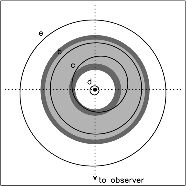
Figure 4: Architecture of the GJ 876 system. The conservative HZ is shown in light grey, the optimistic HZ comprises both the light grey and dark grey regions. Planets b and c spend their entire orbits in the optimistic HZ. Planet b spends its entire orbit in the conservative HZ, whereas planet c spends 68.5% of its orbital period in it. For details, see §3, §4.6, and Table 4. Orbital parameters for the planets are taken from Rivera et al. (2010b). For scale: the size of the box is 0.8 AU $\times$ 0.8 AU.

4.7 HD 1461

HD 1461 hosts two super-Earths in close proximity to both the star and each other: a 7.6 Earth-mass planet in a 5.8-day orbit (Rivera et al., 2010a) and a 5.9 Earth-mass planet in a 13.5-day orbit (Mayor et al., 2011, both are minimum masses). Their semi-major axes are 0.063 and 0.112 AU, respectively, all well inside HD 1461’s HZ, whose inner optimistic/conservative boundary is at 0.83 AU / 1.10 AU.

Our radius estimate of $1.1987\pm 0.0275R_{\odot}$ is larger at the $>2\sigma$ level than both radius estimates in the literature: $1.11\pm 0.04R_{\odot}$ (Takeda, 2007) and $1.0950\pm 0.0260R_{\odot}$ (Valenti & Fischer, 2005).

We measure an effective temperature for HD 1461 to be $5486\pm 52$ K, which falls below all of the many temperature estimates in the literature for HD 1461 – a sensible consequence given that our radius is larger than literature estimates. The Soubiran et al. (2010) catalog alone has 13 different $T_{\rm eff}$ values, ranging from 5683 to 5929 K. Additionally, we find temperature estimates of 5688 K (Holmberg et al., 2009), $5666\pm 42$ K (Prugniel et al., 2011), and $5588\pm 64$ K (Koleva & Vazdekis, 2012) .

We use the $Y^{2}$ isochrones following the method described in Section 3.2 to derive and age and mass of HD 1461. We obtain a mass of $0.94M_{\odot}$ and an age of 13.8 Gyr.

4.8 HD 7924

The super-Earth ($M\sin i=9.26M_{\earth}$) orbits HD 7924 at a period of 5.4 days and at a semi-major axis of 0.057 AU (Howard et al., 2009). The inner boundary of the optimistic/conservative HD 7924 system is at 0.47 AU / 0.62 AU from the star, well beyond the planetary orbit.

The radius of HD 7924 has been estimated to be $R=0.78\pm 0.02R_{\odot}$ (Takeda, 2007), which is identical to our direct measurement of $R=0.7821R_{\odot}$. The radius estimate of $R=0.754R_{\odot}$ (Valenti & Fischer, 2005) is slightly below but consistent with our value.

Our effective temperature measurement $T_{\rm eff}=5075$ K falls into the middle of a large effective temperature range present in the literature for HD 7924: $4550$ K (Lafrasse et al., 2010a), 4750 K (Wright et al., 2003), $5111^{+113}_{-128}$ K (Ammons et al., 2006), 5121 to 5177 K (6 entries; Soubiran et al. 2010), 5177 K (Petigura & Marcy, 2011), 5177 K (Valenti & Fischer, 2005), $5153\pm 5.8$ K (Kovtyukh et al., 2004), 5165 K (Mishenina et al., 2008, 2012).

Our derived mass from Equation 2 is $M=0.81M_{\odot}$.

4.9 HD 33564

HD 33564 hosts a $M\sin i=9.1M_{Jup}$ planet in an eccentric 388-day orbit (Galland et al., 2005) and an orbital semi-major axis of 1.1 AU. Since the orbital eccentricity is 0.34, its apastron distance is $r_{ap}=(1+e)a=1.47$ AU. While the conservative HZ is located beyond HD 33564b’s orbit, the planet spends around 43% of its orbital duration inside the optimistic HZ, whose inner edge is at 1.31 AU. HD 33564’s system architecture is shown in Figure 5.

We measure HD 33564’s radius to be $1.4712\pm 0.0219R_{\odot}$. This is consistent with the previous estimate based on SED fitting by van Belle & von Braun (2009) of $R=1.45\pm 0.03R_{\odot}$.

Our value for the effective temperature of HD 33564 is $6346\pm 44$ K, which is largely consistent with the considerable number of estimates available in the literature: $T_{\rm eff}=6440$ K (Wright et al., 2003), 6302 K (Marsakov & Shevelev, 1995), $6597^{+17}_{-708}$ K (Ammons et al., 2006), $6307-6554$ K (3 entries; Soubiran et al. 2010), $6250\pm 150$ K (Butler et al., 2006), $6531\pm 70$ K (van Belle & von Braun, 2009), 6456 K (Allende Prieto & Lambert, 1999), 6233 K (Schröder et al., 2009), $6379\pm 80$ K (Casagrande et al., 2011), 6307 K (Eiroa et al., 2013), 6394 K (Gray et al., 2003), 6250 K (Dodson-Robinson et al., 2011), and $6554\pm 93$ K (Gonzalez et al., 2010).

We estimate a mass of HD 33564 to be $1.31M_{\odot}$ at an isochronal age of $2.2$ Gyr.

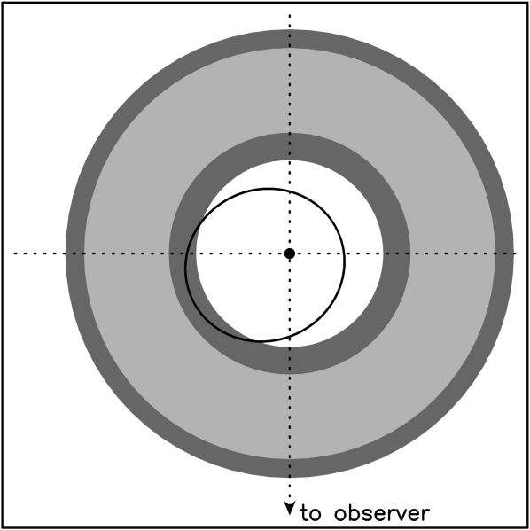
Figure 5: Architecture of the HD 33564 system. The conservative HZ is shown in light grey, the optimistic HZ comprises both the light grey and dark grey regions. The planet in orbit around HD 33564 spends $\sim$ 43% of its orbital period in the optimistic HZ. For details, see §3, §4.9, and Table 4. Orbital parameters are from Galland et al. (2005). The size of the box is 7 AU $\times$ 7 AU.

4.10 HD 107383 (= 11 Com)

The giant star HD 107383 has a substellar-mass companion in an eccentric 328-day orbit at a semi-major axis of 1.29 AU (Liu et al., 2008). Since HD 107383’s luminosity is more than 100 times that of the sun, however, its optimistic/conservative HZ’s inner boundary is at 8.19 AU / 10.83 AU, well beyond even the apastron of the known companion.

Our radius estimate for the giant star HD 107383 is $15.78\pm 0.34R_{\odot}$ – no previous radius estimates appear in the literature for this star. We measure an effective temperature for HD 107383 to be $4705\pm 24$ K, which falls into the middle of previously published values: 4900 K (Wright et al., 2003), $4717^{+381}_{-283}$ K (Ammons et al., 2006), 4690 K (McWilliam, 1990), 4880 K (Hekker & Meléndez, 2007), 4690 K, (Valdes et al., 2004), 4804 K (Schiavon, 2007), $4806\pm 34$ K (Wu et al., 2011), 4690 K (Manteiga et al., 2009), and 4873 K (Luck & Heiter, 2007).

The evolutionary status and consequently the luminosity of this K0 giant are located outside of the range of the $Y^{2}$ isochrones. In addition, the star is evolved, and thus, Equation 2 is not applicable. We therefore cannot calculate its age or mass.

4.11 HD 210702

HD 210702 hosts a $M\sin i=1.9M_{Jup}$ planet in a low-eccentricity, 355-day orbit (Johnson et al., 2007). With a semi-major axis of 1.2 AU, the planet does not enter the system conservative or optimistic HZs, even at apastron.

We measure HD 210702’s radius and $T_{\rm eff}$ to be $5.2314\pm 0.1171R_{\odot}$ and $4780\pm 18$ K, respectively, which is consistent with the interferometric (CHARA $K^{\prime}$-band) values published in Baines et al. (2009, $5.17\pm 0.15R_{\odot}$ and $4859\pm 62$ K), as well as the radius estimated in the XO-Rad catalog of van Belle & von Braun (2009, $5.20\pm 0.31R_{\odot}$). Allende Prieto & Lambert (1999) quote 5.13 $R_{\odot}$ and 4897 K (with error estimates for all stars in their catalog of 6% in radius and 2% in $T_{\rm eff}$) – also consistent with our direct values. Other estimates from Johnson et al. (2007, $4.45\pm 0.07R_{\odot}$ and $5510\pm 44$ K) and Maldonado et al. (2013, $4.7R_{\odot}$ and 4993 K) are lower in radius and higher in effective temperature than our directly determined values.

Application of the $Y^{2}$ isochrones with input values from Table 4 for HD 210702 returns a stellar age of 5 Gyr and a mass of 1.29 $M_{\odot}$.

5 Summary and Conclusion

A very large fraction of the information on extrasolar planets that has been gathered over the course of the last 20 years is purely due to the study of the effects that the planets have on their respective parent stars. That is, the star’s light is used to characterize the planetary system. In addition, the parent star dominates any exoplanet system as the principal energy source and mass repository. Finally, physical parameters of planets are almost always direct functions of their stellar counterparts. These aspects assign a substantial importance to studying the stars themselves: one at best only understands the planet as well as one understands the parent star.

In this paper, we characterize eleven exoplanet host star systems with a wide range in radius and effective temperature, based on a 3.5-year long observing survey with CHARA’s Classic beam combiner. For the systems with previously published direct diameters ($\rho$ CrB, GJ 614, and HD 210702), we provide updates based on increased data quantity and improved performance by the array. For the rest of the systems, only indirectly determined values for radius and effective temperature are present in the literature (if any exist at all). Our thus determined stellar astrophysical parameters make it possible to place our sample of exoplanet host stars onto an empirical Hertzsprung-Russell (H-R) Diagram. In Figure 6, we show our targets along with interferometrically determined parameters of previously published exoplanet hosts and other main-sequence stars with diameter uncertainties of less than 5%.

Due to the relatively low number of stars per spectral type in our sample, and due to the large variance among radius and temperature values quoted in the literature, it is impossible to quantify trends in terms of how indirectly determined values compare with direct counterparts as a function of spectral type, such as the ones documented in Boyajian et al. (2013). For the latest spectral type in our sample, and arguably the most interesting system in terms of exoplanet science, GJ 876, our directly determined stellar radius is significantly ($>20\%$) larger than commonly used literature equivalents (§4.6).

We use our directly determined stellar properties to calculate stellar mass and age wherever possible, though the associated uncertainties are large for the KM dwarfs (§3.2). Calculations of system HZ locations and boundaries, based on stellar luminosity and effective temperature, show that (1) GJ 876 hosts two planets who spend all or large parts of their orbital duration in the system HZ, whereas (2) the planet orbiting HD 33564 spends a small part of its period in the stellar HZ as its elliptical orbit causes it to periodically dip into it around apastron passage.

CHARA’s continously improving performance in both sensitivity and spatial resolution increasingly enables the direct measurements of stellar radii and effective temperatures further and further into the low-mass regime to provide comparison to stellar parameters derived by indirect methods, and indeed calibration of these methods themselves.

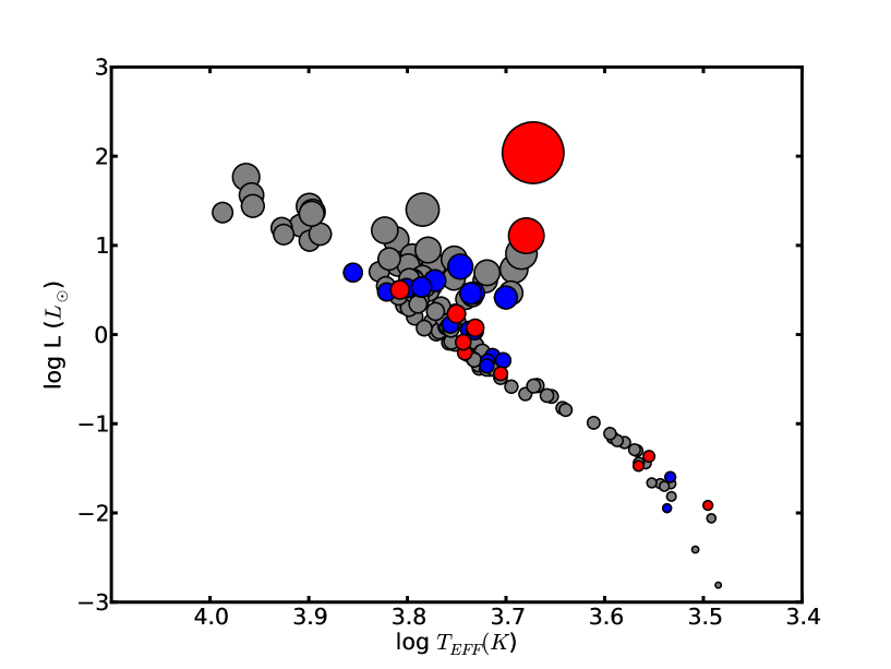
Figure 6: Empirical H-R Diagram for all main-sequence stars with interferometrically determined radii whose random uncertainties are smaller than 5%, as published and compiled in Boyajian et al. (2012b, 2013). The diameter of each data point is representative of the respective stellar radius. Error bars in effective temperature and luminosity are smaller than the size of the data points. Previously published exoplanet host stars are identified in blue (Kervella et al., 2003; Baines et al., 2008b, 2009; van Belle & von Braun, 2009; von Braun et al., 2011a, b, 2012; Boyajian et al., 2013; Henry et al., 2013). The exoplanet host stars that are presented in this work are shown in red. Stars that do not host any published exoplanets are shown in grey.

References

- Akeson et al. (2013) Akeson R. L. et al., 2013, PASP, 125, 989
- Allende Prieto & Lambert (1999) Allende Prieto C., Lambert D. L., 1999, A&A, 352, 555
- Ammons et al. (2006) Ammons S. M., Robinson S. E., Strader J., Laughlin G., Fischer D., Wolf A., 2006, ApJ, 638, 1004
- Anderson & Francis (2011) Anderson E., Francis C., 2011, VizieR Online Data Catalog, 5137, 0
- Anderson & Francis (2012) Anderson E., Francis C., 2012, Astronomy Letters, 38, 331
- Argue (1963) Argue A. N., 1963, MNRAS, 125, 557
- Baines et al. (2008a) Baines E. K., McAlister H. A., ten Brummelaar T. A., Turner N. H., Sturmann J., Sturmann L., Ridgway S. T., 2008a, ApJ, 682, 577
- Baines et al. (2009) Baines E. K., McAlister H. A., ten Brummelaar T. A., Sturmann J., Sturmann L., Turner N. H., Ridgway S. T., 2009, ApJ, 701, 154
- Baines et al. (2008b) Baines E. K., McAlister H. A., ten Brummelaar T. A., Turner N. H., Sturmann J., Sturmann L., Goldfinger P. J., Ridgway S. T., 2008b, ApJ, 680, 728
- Baines et al. (2010) Baines E. K. et al., 2010, AJ, 140, 167
- Beichman et al. (1988) Beichman C. A., Neugebauer G., Habing H. J., Clegg P. E., Chester T. J., eds, 1988, Infrared astronomical satellite (IRAS) catalogs and atlases. Volume 1: Explanatory supplement, Vol. 1
- Bessel (1990) Bessel M. S., 1990, A&AS, 83, 357
- Bessell (2000) Bessell M. S., 2000, PASP, 112, 961
- Bonneau et al. (2006) Bonneau D. et al., 2006, A&A, 456, 789
- Bonneau et al. (2011) Bonneau D., Delfosse X., Mourard D., Lafrasse S., Mella G., Cetre S., Clausse J. M., Zins G., 2011, A&A, 535, A53
- Boyajian et al. (2012a) Boyajian T. S. et al., 2012a, ApJ, 746, 101
- Boyajian et al. (2012b) Boyajian T. S. et al., 2012b, ApJ, 757, 112
- Boyajian et al. (2013) Boyajian T. S. et al., 2013, ApJ, 771, 40
- Bryden et al. (2009) Bryden G. et al., 2009, ApJ, 705, 1226
- Burnashev (1985) Burnashev B. I., 1985, Bulletin Crimean Astrophysical Observatory, 66, 152
- Butler et al. (2003) Butler R. P., Marcy G. W., Vogt S. S., Fischer D. A., Henry G. W., Laughlin G., Wright J. T., 2003, ApJ, 582, 455
- Butler et al. (2006) Butler R. P. et al., 2006, ApJ, 646, 505
- Casagrande et al. (2011) Casagrande L., Schönrich R., Asplund M., Cassisi S., Ramírez I., Meléndez J., Bensby T., Feltzing S., 2011, A&A, 530, A138
- Cernis et al. (1989) Cernis K., Meistas E., Straizys V., Jasevicius V., 1989, Vilnius Astronomijos Observatorijos Biuletenis, 84, 9
- Claret (2000) Claret A., 2000, A&A, 363, 1081
- Clark & McClure (1979) Clark J. P. A., McClure R. D., 1979, PASP, 91, 507
- Correia et al. (2010) Correia A. C. M. et al., 2010, A&A, 511, A21
- Cousins & Stoy (1962) Cousins A. W. J., Stoy R. H., 1962, Royal Greenwich Observatory Bulletins, 64, 103
- Cutri et al. (2003) Cutri R. M. et al., 2003, The 2MASS All Sky Catalog of Point Sources. Pasadena: IPAC
- Dean (1981) Dean J. F., 1981, South African Astronomical Observatory Circular, 6, 10
- Demarque et al. (2004) Demarque P., Woo J. H., Kim Y. C., Yi S. K., 2004, ApJS, 155, 667
- Dodson-Robinson et al. (2011) Dodson-Robinson S. E., Beichman C. A., Carpenter J. M., Bryden G., 2011, AJ, 141, 11
- Ecuvillon et al. (2006) Ecuvillon A., Israelian G., Santos N. C., Shchukina N. G., Mayor M., Rebolo R., 2006, A&A, 445, 633
- Eiroa et al. (2013) Eiroa C. et al., 2013, A&A, 555, A11
- Endl et al. (2008) Endl M., Cochran W. D., Wittenmyer R. A., Boss A. P., 2008, ApJ, 673, 1165
- Erro (1971) Erro B. I., 1971, Boletin del Instituto de Tonantzintla, 6, 143
- Forveille et al. (2009) Forveille T. et al., 2009, A&A, 493, 645
- Fuhrmann et al. (1998) Fuhrmann K., Pfeiffer M. J., Bernkopf J., 1998, A&A, 336, 942
- Galland et al. (2005) Galland F., Lagrange A. M., Udry S., Chelli A., Pepe F., Beuzit J. L., Mayor M., 2005, A&A, 444, L21
- Gezari et al. (1999) Gezari D. Y., Pitts P. S., Schmitz M., 1999, VizieR Online Data Catalog, 2225, 0
- Glushneva et al. (1998) Glushneva I. N. et al., 1998, VizieR Online Data Catalog, 3207, 0
- Golay (1972) Golay M., 1972, Vistas in Astronomy, 14, 13
- Gonzalez et al. (2010) Gonzalez G., Carlson M. K., Tobin R. W., 2010, MNRAS, 403, 1368
- Gray et al. (2003) Gray R. O., Corbally C. J., Garrison R. F., McFadden M. T., Robinson P. E., 2003, AJ, 126, 2048
- Häggkvist & Oja (1966) Häggkvist L., Oja T., 1966, Arkiv for Astronomi, 4, 137
- Häggkvist & Oja (1970) Häggkvist L., Oja T., 1970, A&AS, 1, 199
- Haggkvist & Oja (1987) Haggkvist L., Oja T., 1987, A&AS, 68, 259
- Hanbury Brown et al. (1974) Hanbury Brown R., Davis J., Lake R. J. W., Thompson R. J., 1974, MNRAS, 167, 475
- Heiter & Luck (2003) Heiter U., Luck R. E., 2003, AJ, 126, 2015
- Hekker & Meléndez (2007) Hekker S., Meléndez J., 2007, A&A, 475, 1003
- Henry et al. (2013) Henry G. W. et al., 2013, ApJ, 768, 155
- Holmberg et al. (2009) Holmberg J., Nordström B., Andersen J., 2009, A&A, 501, 941
- Houdebine (2010) Houdebine E. R., 2010, MNRAS, 407, 1657
- Houdebine (2012) Houdebine E. R., 2012, MNRAS, 421, 3189
- Howard et al. (2009) Howard A. W. et al., 2009, ApJ, 696, 75
- Huber et al. (2012) Huber D. et al., 2012, ApJ, 760, 32
- Iriarte (1971) Iriarte B., 1971, Boletin de los Observatorios Tonantzintla y Tacubaya, 6, 143
- Jasevicius et al. (1990) Jasevicius V., Kuriliene G., Strazdaite V., Kazlauskas A., Sleivyte J., Cernis K., 1990, Vilnius Astronomijos Observatorijos Biuletenis, 85, 50
- Jenkins et al. (2009) Jenkins J. S., Ramsey L. W., Jones H. R. A., Pavlenko Y., Gallardo J., Barnes J. R., Pinfield D. J., 2009, ApJ, 704, 975
- Johnson & Knuckles (1957) Johnson H. L., Knuckles C. F., 1957, ApJ, 126, 113
- Johnson & Mitchell (1975) Johnson H. L., Mitchell R. I., 1975, Rev. Mexicana Astron. Astrofis., 1, 299
- Johnson et al. (1966) Johnson H. L., Mitchell R. I., Iriarte B., Wisniewski W. Z., 1966, Communications of the Lunar and Planetary Laboratory, 4, 99
- Johnson et al. (2007) Johnson J. A. et al., 2007, ApJ, 665, 785
- Johnson et al. (2010) Johnson J. A. et al., 2010, PASP, 122, 149
- Jones et al. (1981) Jones D. H. P., Sinclair J. E., Alexander J. B., 1981, MNRAS, 194, 403
- Kane & Gelino (2012) Kane S. R., Gelino D. M., 2012, PASP, 124, 323
- Kane et al. (2013) Kane S. R., Barclay T., Gelino D. M., 2013, ApJ, 770, L20
- Kasting et al. (1993) Kasting J. F., Whitmire D. P., Reynolds R. T., 1993, Icarus, 101, 108
- Kazlauskas et al. (2005) Kazlauskas A., Boyle R. P., Philip A. G. D., Straižys V., Laugalys V., Černis K., Bartašiūtė S., Sperauskas J., 2005, Baltic Astronomy, 14, 465
- Kervella et al. (2003) Kervella P., Thévenin F., Morel P., Bordé P., Di Folco E., 2003, A&A, 408, 681
- Kharitonov et al. (1988) Kharitonov A. V., Tereshchenko V. M., Knjazeva L. N., 1988, The spectrophotometric catalogue of stars
- Kilkenny et al. (2007) Kilkenny D., Koen C., van Wyk F., Marang F., Cooper D., 2007, MNRAS, 380, 1261
- Kim et al. (2002) Kim Y. C., Demarque P., Yi S. K., Alexander D. R., 2002, ApJS, 143, 499
- Koen et al. (2002) Koen C., Kilkenny D., van Wyk F., Cooper D., Marang F., 2002, MNRAS, 334, 20
- Koen et al. (2010) Koen C., Kilkenny D., van Wyk F., Marang F., 2010, MNRAS, 403, 1949
- Koleva & Vazdekis (2012) Koleva M., Vazdekis A., 2012, A&A, 538, A143
- Kopparapu et al. (2013a) Kopparapu R. K. et al., 2013a, ApJ, 770, 82
- Kopparapu et al. (2013b) Kopparapu R. K. et al., 2013b, ApJ, 765, 131
- Kornilov et al. (1991) Kornilov V. G., Volkov I. M., Zakharov A. I., Kozyreva L. N., Kornilova L. N., et al., 1991, Trudy Gosudarstvennogo Astronomicheskogo Instituta, 63, 4
- Kovtyukh et al. (2004) Kovtyukh V. V., Soubiran C., Belik S. I., 2004, A&A, 427, 933
- Kozok (1985) Kozok J. R., 1985, A&AS, 61, 387
- Lafrasse et al. (2010a) Lafrasse S., Mella G., Bonneau D., Duvert G., Delfosse X., Chelli A., 2010a, VizieR Online Data Catalog, 2300, 0
- Lafrasse et al. (2010b) Lafrasse S., Mella G., Bonneau D., Duvert G., Delfosse X., Chesneau O., Chelli A., 2010b, in Society of Photo-Optical Instrumentation Engineers (SPIE) Conference Series. Society of Photo-Optical Instrumentation Engineers (SPIE) Conference Series, Vol. 7734
- Laughlin et al. (2005) Laughlin G., Butler R. P., Fischer D. A., Marcy G. W., Vogt S. S., Wolf A. S., 2005, ApJ, 622, 1182
- Lawler et al. (2009) Lawler S. M. et al., 2009, ApJ, 705, 89
- Liu et al. (2008) Liu Y. J. et al., 2008, ApJ, 672, 553
- Luck & Heiter (2007) Luck R. E., Heiter U., 2007, AJ, 133, 2464
- Maldonado et al. (2013) Maldonado J., Villaver E., Eiroa C., 2013, A&A, 554, A84
- Manteiga et al. (2009) Manteiga M., Carricajo I., Rodríguez A., Dafonte C., Arcay B., 2009, AJ, 137, 3245
- Markwardt (2009) Markwardt C. B., 2009, in D. A. Bohlender, D. Durand, & P. Dowler, ed., Astronomical Society of the Pacific Conference Series. Astronomical Society of the Pacific Conference Series, Vol. 411, pp. 251–+
- Marsakov & Shevelev (1995) Marsakov V. A., Shevelev Y. G., 1995, Bulletin d’Information du Centre de Donnees Stellaires, 47, 13
- Mayor et al. (2011) Mayor M. et al., 2011, ArXiv e-prints
- McClure & Forrester (1981) McClure R. D., Forrester W. T., 1981, Publications of the Dominion Astrophysical Observatory Victoria, 15, 439
- McWilliam (1990) McWilliam A., 1990, ApJS, 74, 1075
- Mermilliod (1986) Mermilliod J. C., 1986, Catalogue of Eggen’s UBV data., 0 (1986), 0
- Mishenina et al. (2008) Mishenina T. V., Soubiran C., Bienaymé O., Korotin S. A., Belik S. I., Usenko I. A., Kovtyukh V. V., 2008, A&A, 489, 923
- Mishenina et al. (2012) Mishenina T. V., Soubiran C., Kovtyukh V. V., Katsova M. M., Livshits M. A., 2012, A&A, 547, A106
- Morales et al. (2008) Morales J. C., Ribas I., Jordi C., 2008, A&A, 478, 507
- Mould & Hyland (1976) Mould J. R., Hyland A. R., 1976, ApJ, 208, 399
- Mumford (1956) Mumford G. S., 1956, AJ, 61, 213
- Noyes et al. (1997) Noyes R. W., Jha S., Korzennik S. G., Krockenberger M., Nisenson P., Brown T. M., Kennelly E. J., Horner S. D., 1997, ApJ, 483, L111
- Oja (1996) Oja T., 1996, Baltic Astronomy, 5, 103
- Olsen (1994) Olsen E. H., 1994, A&AS, 106, 257
- Olson (1974) Olson E. C., 1974, AJ, 79, 1424
- Persson et al. (1977) Persson S. E., Aaronson M., Frogel J. A., 1977, AJ, 82, 729
- Petigura & Marcy (2011) Petigura E. A., Marcy G. W., 2011, ApJ, 735, 41
- Pickles (1998) Pickles A. J., 1998, PASP, 110, 863
- Prugniel et al. (2011) Prugniel P., Vauglin I., Koleva M., 2011, A&A, 531, A165
- Ramírez & Meléndez (2005) Ramírez I., Meléndez J., 2005, ApJ, 626, 465
- Rivera et al. (2010a) Rivera E. J., Butler R. P., Vogt S. S., Laughlin G., Henry G. W., Meschiari S., 2010a, ApJ, 708, 1492
- Rivera et al. (2010b) Rivera E. J., Laughlin G., Butler R. P., Vogt S. S., Haghighipour N., Meschiari S., 2010b, ApJ, 719, 890
- Rojas-Ayala et al. (2012) Rojas-Ayala B., Covey K. R., Muirhead P. S., Lloyd J. P., 2012, ApJ, 748, 93
- Sanders (1966) Sanders W. L., 1966, AJ, 71, 719
- Schiavon (2007) Schiavon R. P., 2007, ApJS, 171, 146
- Schneider et al. (2011) Schneider J., Dedieu C., Le Sidaner P., Savalle R., Zolotukhin I., 2011, A&A, 532, A79
- Schröder et al. (2009) Schröder C., Reiners A., Schmitt J. H. M. M., 2009, A&A, 493, 1099
- Selsis et al. (2007) Selsis F., Kasting J. F., Levrard B., Paillet J., Ribas I., Delfosse X., 2007, A&A, 476, 1373
- Skiff (1994) Skiff B. A., 1994, Information Bulletin on Variable Stars, 3984, 1
- Soubiran et al. (2010) Soubiran C., Le Campion J. F., Cayrel de Strobel G., Caillo A., 2010, A&A, 515, A111
- Sperauskas et al. (1981) Sperauskas J., Bartkevicius A., Zdanavicius K., 1981, Vilnius Astronomijos Observatorijos Biuletenis, 58, 3
- Stauffer & Hartmann (1986) Stauffer J. R., Hartmann L. W., 1986, ApJS, 61, 531
- Straizys (1970) Straizys V., 1970, Dissertation Thesis
- Takeda et al. (2007) Takeda G., Ford E. B., Sills A., Rasio F. A., Fischer D. A., Valenti J. A., 2007, ApJS, 168, 297
- Takeda (2007) Takeda Y., 2007, Publications of the Astronomical Society of Japan, 59, 335
- Tanner et al. (2009) Tanner A., Beichman C., Bryden G., Lisse C., Lawler S., 2009, ApJ, 704, 109
- ten Brummelaar et al. (2005) ten Brummelaar T. A. et al., 2005, ApJ, 628, 453
- The et al. (1984) The P. S., Steenman H. C., Alcaino G., 1984, A&A, 132, 385
- Trilling et al. (2008) Trilling D. E. et al., 2008, ApJ, 674, 1086
- Valdes et al. (2004) Valdes F., Gupta R., Rose J. A., Singh H. P., Bell D. J., 2004, ApJS, 152, 251
- Valenti & Fischer (2005) Valenti J. A., Fischer D. A., 2005, ApJS, 159, 141
- van Belle & van Belle (2005) van Belle G. T., van Belle G., 2005, PASP, 117, 1263
- van Belle & von Braun (2009) van Belle G. T., von Braun K., 2009, ApJ, 694, 1085
- van Leeuwen (2007) van Leeuwen F., 2007, Hipparcos, the New Reduction of the Raw Data. Hipparcos, the New Reduction of the Raw Data. By Floor van Leeuwen, Institute of Astronomy, Cambridge University, Cambridge, UK Series: Astrophysics and Space Science Library, Vol. 350 20 Springer Dordrecht
- Vogt et al. (2010) Vogt S. S. et al., 2010, ApJ, 708, 1366
- von Braun et al. (2011a) von Braun K. et al., 2011a, ApJ, 740, 49
- von Braun et al. (2011b) von Braun K. et al., 2011b, ApJ, 729, L26+
- von Braun et al. (2012) von Braun K. et al., 2012, ApJ, 753, 171
- Weis (1984) Weis E. W., 1984, ApJS, 55, 289
- Weis (1986) Weis E. W., 1986, AJ, 91, 626
- Weis (1987) Weis E. W., 1987, AJ, 93, 451
- Weis (1993) Weis E. W., 1993, AJ, 105, 1962
- Weis (1996) Weis E. W., 1996, AJ, 112, 2300
- Weis & Upgren (1982) Weis E. W., Upgren A. R., 1982, PASP, 94, 821
- Wright et al. (2003) Wright C. O., Egan M. P., Kraemer K. E., Price S. D., 2003, AJ, 125, 359
- Wright et al. (2011a) Wright J. T. et al., 2011a, PASP, 123, 412
- Wright et al. (2011b) Wright N. J., Drake J. J., Mamajek E. E., Henry G. W., 2011b, ApJ, 743, 48
- Wu et al. (2011) Wu Y., Singh H. P., Prugniel P., Gupta R., Koleva M., 2011, A&A, 525, A71
- Yi et al. (2001) Yi S., Demarque P., Kim Y. C., Lee Y. W., Ree C. H., Lejeune T., Barnes S., 2001, ApJS, 136, 417
- Yoss & Griffin (1997) Yoss K. M., Griffin R. F., 1997, Journal of Astrophysics and Astronomy, 18, 161
- Zakhozhaj (1979) Zakhozhaj V. A., 1979, Vestnik Khar’kovskogo Universiteta, 190, 52