Modeling association between DNA copy number and gene expression with constrained piecewise linear regression splines

Abstract

DNA copy number and mRNA expression are widely used data types in cancer studies, which combined provide more insight than separately. Whereas in existing literature the form of the relationship between these two types of markers is fixed a priori, in this paper we model their association. We employ piecewise linear regression splines (PLRS), which combine good interpretation with sufficient flexibility to identify any plausible type of relationship. The specification of the model leads to estimation and model selection in a constrained, nonstandard setting. We provide methodology for testing the effect of DNA on mRNA and choosing the appropriate model. Furthermore, we present a novel approach to obtain reliable confidence bands for constrained PLRS, which incorporates model uncertainty. The procedures are applied to colorectal and breast cancer data. Common assumptions are found to be potentially misleading for biologically relevant genes. More flexible models may bring more insight in the interaction between the two markers.

, , and

t1Supported by the Center for Medical Systems Biology (CMSB), established by the Netherlands Genomics Initiative/Netherlands Organization for Scientific Research (NGI/NWO).

1 Introduction

The genetic material of the human cancer cells often exhibits abnormalities, of which DNA copy number aberrations are a prime example. These aberrations comprise gains and losses of chromosome pieces that are highly variable in size. Thereby, all or parts of a chromosome may have more or less than the two copies received from the parents. Abnormal DNA copy numbers (different from two) may alter expression levels of mRNA transcripts (encoding for functional proteins) that map to the aberration’s genomic location. Apart from being concordant (copy number tends to correlate positively with expression level), the form of this association is not established and may even vary per gene. In this paper we use high-throughput data available for tissue-specific samples from unrelated patients to study the relationship between copy number (DNA) and gene expression (mRNA). We employ a wide class of interpretable models to reflect the biological mechanism operating between these two molecular levels and identify relevant markers that may serve as therapeutic targets.

DNA copy number aberrations are often measured by array comparative genomic hybridization (aCGH) [Pinkel and Albertson (2005)]. This measuring device is similar to expression microarrays, which measure expression levels of thousands of genes simultaneously but interrogate DNA rather than RNA. Thereby, both profiling experiments produce a continuous value for every element/probe on the array: a $\log_{2}$-value of optical fluorescence intensity. As experiments appear similar, types of information differ and so are their subsequent treatment. To understand the specific nature of these data, we include a description of their processing.

Normalization of mRNA expression profiles [Quackenbush (2002)] consists in removing experimental artifacts (such as array differences, means, scales) and yields, for every gene on each array, a continuous value (normalized $\log_{2}$-value) which represents the amount of the gene’s transcript present in the sample. Preprocessing of copy number/aCGH profiles aims to characterize the genomic instability of each tumor sample and show deleted/duplicated pieces of chromosomes. Three successive steps (illustrated in Figure 1) are typically executed to recover the aberration states of all probes [van de Wiel et al. (2011)]. Through these steps, the size, genomic position and type of copy number aberrations are determined for all samples. In the first preprocessing step, the normalization of $\log_{2}$-values removes technical or biological artifacts (such as tumor sample contamination, GC content) and makes the data comparable across samples. Next, segmentation partitions the genome of each sample into segments of constant $\log_{2}$-values. These segments are considered a smoothed (and thus de-noised) version of their normalized counterparts. Segmentation is motivated by the biological breakpoint process on the DNA that may cause differential copy number between neighboring locations. Finally, calling assigns an aberration state to each segment. Probabilistic calling, usually based on mixture models, results in a probability distribution over a set of ordered possible types of genomic aberrations (which we will refer to as states), typically comprising “loss” ($<$2 copies), “normal” ($=$2 copies), “gain” (3–4 copies) and “amplification” ($>$4 copies). A state is attributed to each probe using a classification rule on the membership probabilities. Nonprobabilistic calling directly assigns states to segmented values, for example, by using a threshold. Note that larger segmented values almost always correspond to a larger or equal called copy number (see Figure 1). All in all, the three steps of the preprocessing procedure provide distinct, but strongly related, data sets: (1) the normalized, (2) segmented and (3) called aCGH data. While most down-stream analyses use either segmented or called data, we use them jointly.

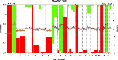
Figure 1: Plot of a copy number/aCGH profile from the breast cancer data set [Neve et al. (2006)] showing the different preprocessing steps. Probes on the array are genomically ordered on the x-axis (only the chromosome number is displayed). Black dots and orange segments indicate the normalized and segmented $\log_{2}$-values (right y-axis), respectively. Bars represent “loss” (red) and “gain” (green and reversed) membership probabilities (left y-axis). Amplifications are indicated by tick marks on the top axis.

Current methodology for integrative genomic studies assumes rather than explores the mathematical form of the relationship between copy number and expression level. The relationship is said to be either linear or stepwise (see examples in Figure 2). A linear relationship is often assumed in combination with segmented aCGH data. For instance, the strength of the DNA-mRNA association is measured by a (modified) correlation coefficient [Salari, Tibshirani and Pollack (2010), Schäfer et al. (2009), Lee, Kong and Park (2008), Lipson et al. (2004)]. Alternatively, a linear regression approach is entertained [Asimit, Andrulis and Bull (2011), Menezes et al. (2009), Gu, Choi and Ghosh (2008)]. Recently published multivariate methods [Jörnsten et al. (2011), Peng et al. (2010), Soneson et al. (2010), van Wieringen, Berkhof and van de Wiel (2010)] also assume linearity. A piecewise DNA-mRNA relationship is considered when using the called aCGH data for integrative analysis. van Wieringen and van de Wiel (2009) and Bicciato et al. (2009) have proposed stepwise methods.

Figure 2: Illustration of the association between DNA and mRNA for three genes in the breast cancer data set [Neve et al. (2006)] used in this study. Segmented copy number is on the x-axis, while gene expression is on the y-axis. Symbols indicate the different states, namely, loss ($\bigtriangledown$), normal ($\bigcirc$) and gain ($\bigtriangleup$). The dashed and “continuous” lines give the fitted linear and stepwise models, respectively.

In this paper we develop model selection for piecewise linear regression splines (PLRS) to decipher how DNA copy number abnormalities alter the mRNA gene expression level. In addition, we propose a statistical test that accounts for model uncertainty in the PLRS context to detect those genes that drive important shifts. The PLRS framework encompasses the linear and stepwise relationships, but provides flexibility, while maintaining good interpretability. In particular, it accommodates differential DNA-mRNA relationships across states. This is biologically plausible, because the cell has various post-transcriptional mechanisms to undo the effects of DNA aberrations. For a given gene, the efficacy of such mechanisms is likely to differ between gains and losses. For example, a gain can directly be compensated by regulatory mechanisms that cause mRNA degradation, such as methylation. On the other hand, a complete loss of both DNA copies (which is more rare than partial loss) cannot be compensated at all.

Segmented and called data are incorporated into the analysis, and biologically motivated constraints are imposed on the model parameters. As this makes model selection and inference nonstandard, we provide methodology for testing the effect of DNA on mRNA within the context of PLRS and for selecting the appropriate model. We also present a novel and computationally inexpensive method for obtaining uniform confidence bands. We apply the proposed methodology to colorectal and breast cancer data sets, where we identify many genes exhibiting nonstandard behavior.

2 Methods

We model the association between DNA copy number and mRNA expression by piecewise linear regression splines (PLRS), with biologically motivated constraints on the coefficients. In this section we address model selection and describe a modified Akaike criterion in this context. Further, we present a method for determining uniform confidence bands, along with a statistical test for the effect of copy number on mRNA expression.

2.1 Model

Consider gene expression and aCGH profiling of $n$ independent tumor samples where for a given gene $\{y_{i},x_{i},s_{i}\}_{i=1}^{n}$ are available, with $y_{i}$ being the normalized mRNA expression ($\log_{2}$ scale), $x_{i}$ the segmented copy number ($\log_{2}$ scale) and $s_{i}$ the copy number state (“loss,” “normal,” “gain” and “amplification,” coded by $-1$, 0, 1 and 2) value of the $i$th observation, respectively. Then, the “full” model with $S$ states (or parts) takes the form

$${y_{i}=f_{\alpha}(x_{i};\theta)+\varepsilon_{i}=\theta_{0}+\theta_{1}x_{i}+\sum_{j=1}^{S-1}{\sum_{d=0}^{1}{\theta_{j,d}(x_{i}-\alpha_{j})_{+}^{d}}}+\varepsilon_{i}}.$$ (1)

Here $\theta=\{\theta_{0},\theta_{1},\theta_{1,0},\ldots,\theta_{S-1,0},\theta_{1,1},\ldots,\theta_{S-1,1}\}$ is a vector of $2\times S$ unknown parameters, the $\varepsilon_{i}$ are independent random variables each normally distributed with mean $0$ and variance $\sigma^{2}$, and $\{\alpha_{j}\}$ are $S-1$ known knots. The quantity $(a)_{+}^{d}$ represents the positive part $\max(a,0)$ of $a$ raised to the power $d$. The number of aberration states $S$ varies across genes. In this study no more than four different aberration states are considered ($S\leq 4$). Below, for the purpose of discussing model (1) we consider the general case $S=4$.

Knots $\{\alpha_{j}\}$ are obtained using data from the calling preprocessing step. Depending on the type of calling, two possibilities present themselves. First, consider nonprobabilistic calling which renders states $\{s_{i}\}_{i=1}^{n}$. Then, $\alpha_{j}$ is taken to be the midpoint of the interval between segmented values $x_{i}$ belonging to consecutive states (method I). This makes the (natural) supposition that the calling values respect the ordering of the segmented values $x_{i}$ and should be reasonably precise if the between-state intervals are small, which is typical (see Figure 2). Second, consider probabilistic calling, which renders membership (or call) probabilities: $(p_{i,-1},p_{i,0},p_{i,1},p_{i,2})$. These reflect the plausibility of the segmented value $x_{i}$ to belong to the states $s_{i}\in\{-1,0,1,2\}$ [van de Wiel et al. (2007)]. Then for $j\in\{1,2,3\}$, we estimate $\alpha_{j}$ (method II) by

$${\hat{\alpha}_{j}=\mathop{\operatorname{arg\,max}}_{\alpha\in\mathbb{R}}\sum_{i=1}^{n}{p_{i,j(i,\alpha)}}},\qquad j(i,\alpha)=\cases{j-2,&\quad$\mbox{if $x_{i}\leq\alpha$},$\vspace*{2pt}\cr j-1,&\quad$\mbox{if $x_{i}>\alpha$}$.}$$ (2)

For instance, $\alpha_{2}$ is the knot between states 0 and 1. To determine its position, we select for each sample its plausibility $p_{i,0}$ of belonging to state 0 (when $x_{i}\leq\alpha_{2}$) or $p_{i,1}$ of belonging to state 1 (when $x_{i}>\alpha_{2}$), and add over all samples. We select $\alpha_{2}$ to maximize the sum. The maximum may not be unique but described by a small interval; in such a case, we use the corresponding midpoint. This method may be preferable as it accounts for the uncertainty of the calling states. The two methods taken here use data as provided by available calling algorithms. Proposed models for this preprocessing step typically depend on data from all samples, which stabilizes the estimation of $\alpha_{j}$. Furthermore, knots are to be interpreted as boundaries between the (ordered) states $\{-1,0,1,2\}$, which gives us strong a priori knowledge as to their placing (see Figure 2). Together, these two arguments support our approach to consider knots in model (1) as being known. In Section 3 of the supplementary material (SM) [Leday et al. (2013)], a simulation shows that standard deviations of $\hat{\alpha}_{j}$ are indeed very small.

Model (1) contains seven basis functions besides the intercept $\theta_{0}$ and hence is quite flexible. Our approach is to select appropriate basis functions ($2^{7}=128$ possible models) and estimate the parameters. The basis functions of degree zero $x\mapsto(x-\alpha)_{+}^{0}$ model discontinuities, and hence allow for a different effect of copy number on expression for each state.

This framework is a natural fundament to test meaningful hypotheses. For example, the hypothesis that for a given state there is an effect of copy number on mRNA can be expressed in terms of a linear function of the parameters being zero ($\sum_{j}{\theta_{j,1}}=0$); a difference between the effects of two adjacent states corresponds to knot deletion. The submodel consisting of piecewise constant functions [without the functions $x\mapsto x$ and $x\mapsto(x-\alpha)_{+}^{1}$] allows testing the difference in expression between states based on discrete genomic information.

To increase biological plausibility, aid interpretation and increase the stability of estimation, we impose a set of linear constraints on the parameters. As it is generally believed that direct causal effects of DNA on mRNA should be positive, we constrain all slopes to be nonnegative. More exactly, we constrain the slope corresponding to the “normal” state to be nonnegative ($\theta_{1}+\theta_{1,1}\geq 0$), while others are forced to be at least equal to the latter (implied by $\theta_{1,1}\leq 0$ for losses, $\theta_{2,1}\geq 0$ for gains and $\theta_{2,1}+\theta_{3,1}\geq 0$ for amplifications). For the same reason we constrain jumps $\theta_{j,0}$ from state to state to be nonnegative. Note that the restrictions adopted here force the slope of the “normal” state to be small or null and make the natural assumption that a normal copy number is not expected to affect (at least severely) gene expression.

The maximum likelihood estimator of the unknown vector of coefficients $\theta$ solves the following convex optimization problem:

$$\mathop{\mathrm{minimize}}_{\theta}(y-\mathbf{X}\theta)^{T}(y-\mathbf{X}\theta)\qquad\mbox{subject to }\mathbf{C}\theta\geq 0.$$ (3)

This can be solved by quadratic programming [Boyd and Vandenberghe (2004)]. The vector $y=\{y_{1},\ldots,y_{n}\}$ denotes the expression signature of a given gene and $\mathbf{X}$ the associated matrix of covariates designed according to (1). The full row-rank matrix $\mathbf{C}$ expresses the constraints that are imposed on the parameters. For the 4-state full model we define $\mathbf{C}$ as the matrix in

$$\pmatrix{0&1&0&1&0&0&0&0\vspace*{2pt}\cr 0&0&0&0&0&1&0&0\vspace*{2pt}\cr 0&0&0&0&0&1&0&1\vspace*{2pt}\cr 0&0&0&-1&0&0&0&0\vspace*{2pt}\cr 0&0&1&0&0&0&0&0\vspace*{2pt}\cr 0&0&0&0&1&0&0&0\vspace*{2pt}\cr 0&0&0&0&0&0&1&0}\pmatrix{\theta_{0}\vspace*{2pt}\cr\theta_{1}\vspace*{2pt}\cr\theta_{1,0}\vspace*{2pt}\cr\theta_{1,1}\vspace*{2pt}\cr\theta_{2,0}\vspace*{2pt}\cr\theta_{2,1}\vspace*{2pt}\cr\theta_{3,0}\vspace*{2pt}\cr\theta_{3,1}}\geq 0.$$ (4)

2.2 Model selection

Given $R$ competing statistical models, with log-likelihoods $\mathcal{L}_{r}(\theta_{r})$ based on a $k_{r}\times 1$ parameter vector $\theta_{r}$ and with corresponding maximum likelihood estimators (MLE) $\hat{\theta}_{r}$, the Akaike information criterion (AIC) selects as best the model that minimizes

$$\mathrm{AIC}_{r}=-\mathcal{L}_{r}(\hat{\theta}_{r})+k_{r}.$$ (5)

This information criterion consists of two parts: the negative maximized log-likelihood, which measures the lack of model fit, and a penalty for model complexity. Although AIC has found wide application, it is less suitable for models that include parameter constraints, as in our situation. It can be adapted as follows.

The original motivation for the criterion [Akaike (1973)] is to choose the model that minimizes the Kullback–Leibler (KL) divergence to the true distribution of the data. Indeed, the criterion $\mathrm{AIC}_{r}$ is (under some conditions) an asymptotically unbiased estimator of this KL divergence. The likelihood at a given parameter is an unbiased estimate of the KL divergence at this parameter, but evaluating it at the maximum likelihood estimator introduces a bias caused by “using the data twice,” which is compensated by the penalty $k_{r}$ [Bozdogan (1987)]. In the constrained case (i.e., subject to $\mathbf{C}\theta\geq 0$) we can follow the same motivation, but must account for a different behavior of the maximum likelihood estimator and the resulting bias. Intuitively, the penalty adjusts for an expected increase in the maximized log-likelihood when variables are added to the model, which is less likely under constraints. The likelihood of violation of the constraints must be taken into account.

Hughes and King (2003) adapted the AIC criterion using the asymptotic distribution of the Wald test statistic. In the constrained situation this statistic is not distributed as a chi-squared random variable anymore, but as a probability weighted mixture of chi-squared random variables [see Chernoff (1954), Gouriéroux, Holly and Monfort (1982), Kodde and Palm (1986) or van der Vaart (1998), Theorem 16.7]. It is of the form (partially inequality constrained Wald statistic)

$${\sum_{h=0}^{p_{r}}{w(p_{r},h)}\chi^{2}(k_{r}-p_{r}+h)},$$ (6)

where $p_{r}$ is the number of inequality constraints and $w(p_{r},h)$ are weights [with $\sum_{h}w(p_{r},h)=1$], which can be interpreted as the probabilities under the null hypothesis that the constrained maximum likelihood estimator $\widetilde{\theta}_{r}$ satisfies $h$ out of $p_{r}$ constraints.

Hughes and King (2003) propose to use the one-sided AIC (OSAIC), which is an asymptotically unbiased estimator of the KL divergence in the presence of one-sided information:

$$\mathrm{OSAIC}_{r}=-\mathcal{L}_{r}(\widetilde{\theta}_{r})+{\sum_{h=0}^{p_{r}}{w(p_{r},h)(k_{r}-p_{r}+h)}}.$$ (7)

Calculating the weights is a combinatorial problem, which aims to determine the probability that the vector $\widetilde{\theta}_{r}$ lies in any face of dimension $h$ [Kudô (1963), Shapiro (1988), Grömping (2010)]. This can be computationally intensive as the number of variables, $k_{r}$, increases [Grömping (2010)]. However, in this study the largest model has eight free parameters (because $S\leq 4$). Therefore, the model selection procedure is still very fast (a couple of seconds).

2.3 Testing

To evaluate the effect of DNA copy number on expression, we test the hypothesis $H_{0}\dvtx\mathbf{C}\theta=0$ against the alternative $H_{1}\dvtx\mathbf{C}\theta\neq 0,\mathbf{C}\theta\geq 0$, that is, we test that all inequality constraints are satisfied as equalities against the possibility that at least one of them is strict. From (4) we observe that all parameters except the intercept $\theta_{0}$ are subject to inequality constraints and that the null hypothesis reduces the model to the intercept.

We employ the likelihood ratio statistic $\mathrm{LR}=2(\mathcal{L}_{1}-\mathcal{L}_{0})$, where $\mathcal{L}_{0}$ and $\mathcal{L}_{1}$ are the maximized log-likelihood under the null and alternative hypotheses, respectively. The test rejects the null hypothesis for large values of

$$\mathop{\operatorname{min}}_{\mathrm{C}\theta\geq 0}(y-\mathbf{X}\theta)^{T}(y-\mathbf{X}\theta)-\mathop{\operatorname{min}}_{\mathrm{C}\theta=0}(y-\mathbf{X}\theta)^{T}(y-\mathbf{X}\theta).$$ (8)

This can be shown [Robertson, Wright and Dykstra (1988)] to be equivalent to rejecting for large values of

$$\overline{\chi}^{2}=(\widetilde{\theta}-\widetilde{\theta}_{=})^{T}\Sigma^{-1}_{\mathbf{X}}(\widetilde{\theta}-\widetilde{\theta}_{=}),$$ (9)

where $\widetilde{\theta}$ and $\widetilde{\theta}_{=}$ are the maximum likelihood estimators under the inequality and the equality constraints, respectively, and $\Sigma_{\mathbf{X}}=\sigma^{2}(\mathbf{X}^{T}\mathbf{X})^{-1}$ is the covariance matrix of the unconstrained least squares estimator. For known error variance $\sigma^{2}$ the chi-bar-squared statistic $\overline{\chi}^{2}$ may be employed with null distribution approximated by a weighted mixture of $\chi^{2}$ distributions [Chernoff (1954), Gouriéroux, Holly and Monfort (1982)]. As $\sigma^{2}$ is typically unknown, we use instead the so-called E-bar-squared statistic [Robertson, Wright and Dykstra (1988), Shapiro (1988), Grömping (2010), Silvapulle and Sen (2005)]

$$\overline{E}^{2}=\frac{(\widetilde{\theta}-\widetilde{\theta}_{=})^{T}\Omega_{\mathbf{X}}^{-1}(\widetilde{\theta}-\widetilde{\theta}_{=})}{(\widetilde{\theta}-\widetilde{\theta}_{=})^{T}\Omega_{\mathbf{X}}^{-1}(\widetilde{\theta}-\widetilde{\theta}_{=})+(y-\mathbf{X}\hat{\theta})^{T}(y-\mathbf{X}\hat{\theta})}.$$ (10)

Here $\Omega_{\mathbf{X}}=\mathbf{X}^{T}\mathbf{X}$. The null distribution of this statistic is a weighted mixture of Beta distributions of the form

$${\sum_{h=0}^{p}{w(p,h)}\mathcal{B}\bigl{(}h/2,(n-p)/2\bigr{)}},$$ (11)

where $p$ is the number of parameters and $\mathcal{B}(a,b)$ refers to a beta distribution with shape parameters $a$ and $b$. The mixing weights are the same as in (6) (applied to the full model); unknown parameters are estimated by their MLEs.

Further details on these test statistics can be found in Shapiro (1988), Robertson, Wright and Dykstra (1988), Silvapulle and Sen (2005).

2.4 Confidence bands

Confidence bands (CBs) for the (spline) function $\mathbf{x}\mapsto f_{\alpha}(\mathbf{x};\theta)$ in equation (1) should take both the model selection procedure [Buckland, Burnham and Augustin (1997)] and the constraints into account.

Initially we implemented a bootstrap procedure [Grömping (2010)], accounting for model uncertainty along the lines of Burnham and Anderson (2002), who propose the construction of so-called unconditional confidence intervals where only the selected model is considered for each bootstrap sample. Unfortunately, simulated coverage probabilities were below (and sometimes far below, e.g., 0.6 instead of 0.95) the nominal level, probably due to the presence of the inequality constraints in our model [Andrews (2000)]. We therefore developed an “exact” alternative based on the E-bar-squared statistic (10), using semidefinite programming to achieve computational efficiency. A simulation study reported in Section 3.2 shows that this approach yields accurate uniform CBs.

2.4.1 Problem formulation

We start by the construction of a joint confidence region for all parameters $\theta$ in the full model, including the intercept $\theta_{0}$, by inverting the likelihood ratio test described previously. Analogously to equation (10), define

$${\overline{E}^{2}(\theta)=\frac{(\widetilde{\theta}-\theta)^{T}\Omega_{\mathbf{X}}^{-1}(\widetilde{\theta}-\theta)}{(\widetilde{\theta}-\theta)^{T}\Omega_{\mathbf{X}}^{-1}(\widetilde{\theta}-\theta)+(y-\mathbf{X}\hat{\theta})^{T}(y-\mathbf{X}\hat{\theta})}}.$$

Then a $(1-\alpha)\%$ confidence region $\mathcal{R}$ for $\theta$ is

$$\mathcal{R}=\bigl{\{}\theta\dvtx\overline{E}^{2}(\theta)\leq\mathcal{Q}_{1-\alpha},\mathbf{C}\theta\geq 0\bigr{\}},$$ (12)

where $\mathcal{Q}_{1-\alpha}$ denotes the $(1-\alpha)$-quantile of the beta mixture distribution in (11). Here we increment the first parameter of the Beta distributions to $(h+1)/2$, because presently we include the intercept as a parameter, whereas before it was free under the null hypothesis. Interval estimation based on inversion of a likelihood ratio statistic is known to possess good properties [Meeker and Escobar (1995), Arnold and Shavelle (1998), Brown, Cai and DasGupta (2003)].

Given the confidence region $\mathcal{R}$, we compute a confidence band by determining for each $\mathbf{x}$ the minimum and maximum values $f_{\alpha}(\mathbf{x};\theta)=\mathbf{x}^{T}\theta$. This means determining

$$\inf_{\theta\in\mathcal{R}}\mathbf{x}^{T}\theta\quad\mbox{and}\quad\sup_{\theta\in\mathcal{R}}\mathbf{x}^{T}\theta.$$

Thus, a simple linear function must be minimized (or maximized) subject to linear and ellipsoidal inequality constraints. In the following section, we show that this (convex) problem can be solved efficiently by semidefinite programming.

2.4.2 Semidefinite programming

A semidefinite program [Vandenberghe and Boyd (1996)] is concerned with the minimization of a linear objective function under the constraint that a linear combination of symmetric matrices is positive semidefinite:

$$\mathop{\mathrm{minimize}}_{y\in\mathbb{R}^{m}}b^{T}y\qquad\mbox{subject to }F(y)=F_{0}+\sum_{i=1}^{m}{y_{i}F_{i}}\succeq 0.$$ (13)

The vector $b\in\mathbb{R}^{m}$ and the symmetric $(n\times n)$ matrices $F_{0},\ldots,F_{m}$ are fixed, and the expression $F(y)\succeq 0$ means that the matrix $F(y)$ is positive semidefinite [i.e., $z^{T}F(y)z\geq 0$, $\forall z\in\mathbb{R}^{n}$]. Because a linear matrix inequality constraint $F(y)\succeq 0$ is convex, the program can be solved efficiently using interior-point methods [Vandenberghe and Boyd (1996)].

We may express the optimization problem of the previous section as a semidefinite program, based on two equivalences, given by Vandenberghe and Boyd (1996) and provided in Appendix B. For convenience, we replace the ellipsoidal constraint $\overline{E}^{2}(\theta)\leq\mathcal{Q}_{1-\alpha}$ by $(M\theta-M\widetilde{\theta})^{T}(M\theta-M\widetilde{\theta})\leq\lambda$, where ${\lambda=(y-\mathbf{X}\hat{\theta})^{T}(y-\mathbf{X}\hat{\theta})\mathcal{Q}_{1-\alpha}/(1-\mathcal{Q}_{1-\alpha})}$ and $\Omega_{\mathbf{X}}^{-1}=M^{T}M$. Given this, the semidefinite program is

$$\mathop{\mathrm{minimize}}_{\theta}\mathbf{x}^{T}\theta\qquad\mbox{subject to }F(\theta)=F_{0}+\sum_{i=1}^{p}{\theta_{i}F_{i}}\succeq 0,$$ (14)

where

$$F_{0}=\pmatrix{0&0\vspace*{2pt}\cr 0&F^{(2)}_{0}},\qquad F_{i}=\pmatrix{F^{(1)}_{i}&0\vspace*{2pt}\cr 0&F^{(2)}_{i}},\qquad i=1,\ldots,p,$$

with the submatrices defined as

$$F^{(1)}_{i}=\operatorname{diag}(c_{i}),\qquad F^{(2)}_{0}=\pmatrix{I&-M\widetilde{\theta}\vspace*{2pt}\cr(-M\widetilde{\theta})^{T}&\lambda}\quad\mbox{and}\quad F^{(2)}_{i}=\pmatrix{0&m_{i}\vspace*{2pt}\cr m_{i}^{T}&0}.$$

Here $m_{i}$ and $c_{i}$ denote the $i$th column vector of the matrices $M$ and $\mathbf{C}$ [the matrix of linear restrictions expressed in (3)], respectively.

The optimization procedure needs to be repeated twice in order to determine the lower and upper bounds on $\mathbf{x}^{T}\theta$. Even though this must next be repeated for every new instance $\mathbf{x}$ to obtain a confidence band, the overall procedure is fast. For instance, for 100 new instances computation on a 2.66 GHz Intel quad-core took less than 12 s (without parallel computing).

3 Simulation

We conducted simulation experiments to: (1) determine the accuracy of estimates as provided by PLRS (Section 3.1); (2) examine the coverage probabilities of the method proposed in Section 2.4 (Section 3.2); and (3) evaluate the performance of the PLRS screening test in detecting associations of various functional forms (Section 3.3).

3.1 Point estimation

The simulation study examined the accuracy of the estimates obtained by fitting piecewise splines or a simple linear model. For simplicity, we consider a two-state model (normal and gain) and the knot was fixed to 0.5. Data were generated according to the following:

• model 1: $y=1+a_{2}(x-0.5)^{1}_{+}$, $a_{2}\in\{0,0.5,1,2,5\}$

• model 2: $y=1+0.5x+(a_{2}-0.5)(x-0.5)^{1}_{+}$, $a_{2}\in\{0,0.5,1,2,5\}$.

The first state (normal) has no or little effect on expression. The linear function is contained in both models, and is found for $a_{2}=0$ and $a_{2}=0.5$, respectively. We generated errors from a normal distribution $\mathcal{N}(0,\sigma^{2})$ where $\sigma\in\{0.1,0.25,0.5,0.75,1\}$. This resulted in 25 cases for each of the two models (5 values of $a_{2}$ times 5 values of $\sigma$). The sample size was set to 80, and the 80 values of $x$ were generated from a uniform distribution $\mathcal{U}(0,1)$.

We were interested in comparing the precision of the estimates of the slope $a_{2}$ when fitting a linear or a piecewise linear model (the latter with a single knot placed at $0.5$; 4 parameters). For each of the 25 cases we repeated the simulation experiment 1000 times and computed the estimator of the slope for both models. Table 1 reports the empirical squared bias and variance over the 1000 repetitions. For clarity only the results for $\sigma=0.25$ and $\sigma=0.75$ are displayed. Complementary results can be found in Section 2 of SM.

Not surprisingly, the piecewise model can capture the relationship well in all cases: the squared bias is small, and the variance never unduly large. On the other hand, the estimate of the slope given by the linear model is strongly biased for larger values of the slope $a_{2}$. As expected, the variance of the PLRS estimate is usually somewhat larger than that of the linear model estimate. However, this difference is much less prominent than for the squared bias. When the data generating process is linear, that is, when $a_{2}=0$ in model 1 and $a_{2}=0.5$ in model 2, the difference between the estimates from the linear and PLRS models is smaller than in the other cases.

The study suggests that, when estimating or testing the effect of DNA copy number on mRNA expression, there is potentially more to lose than to gain (due to misspecification versus overspecification of the model) by applying the linear instead of the piecewise linear spline model.

Table 1: Squared bias and variance (in parentheses) of the slope estimates of the linear and piecewise spline models as a function of the true slope $a_{2}$, noise $\sigma$ and model. In bold: setting for which the true model is linear

		$\bolds{\sigma=0.25}$		$\bolds{\sigma=0.75}$
Model	$\bolds{a_{2}}$	linear	piecewise	linear	piecewise
1	00.	0.002 (0.004)	0.007 (0.012)	0.015 (0.033)	0.047 (0.090)
	0.5	0.070 (0.011)	0.002 (0.039)	0.050 (0.060)	0.000 (0.193)
	10.	0.282 (0.011)	0.004 (0.045)	0.270 (0.081)	0.008 (0.271)
	20.	1.114 (0.011)	0.003 (0.045)	1.124 (0.094)	0.027 (0.339)
	50.	6.962 (0.011)	0.003 (0.042)	6.908 (0.103)	0.022 (0.393)
2	00.	0.060 (0.008)	0.063 (0.009)	0.075 (0.053)	0.124 (0.097)
	0.5	0.000 (0.009)	0.005 (0.019)	0.000 (0.066)	0.030 (0.146)
	10.	0.058 (0.008)	0.000 (0.036)	0.055 (0.070)	0.006 (0.180)
	20.	0.545 (0.008)	0.000 (0.041)	0.521 (0.075)	0.000 (0.289)
	50.	4.782 (0.008)	0.000 (0.046)	4.857 (0.073)	0.004 (0.320)

3.2 Uniform CBs

To study the coverage probabilities of the method proposed in Section 2.4, we simulated data according to the model $y=1+(x-0.5)^{0}_{+}+(x-0.5)^{1}_{+}$, with $x$-values drawn from a uniform distribution $\mathcal{U}(0,1)$. Gaussian errors of standard deviation $\sigma\in\{0.5,1\}$, and three sample sizes $n\in\{20,40,80\}$. For a given data set we computed the confidence band on a grid of 10 equidistant values, for two different significance levels $\alpha\in\{0.05,0.1\}$, and checked whether the 10 corresponding values of the function in the display fall simultaneously into the estimated confidence band. (For computational reasons the simulation was limited to 10 values; we believe that using the continuous range would not have altered the findings.) Table 2 shows the empirical coverage probabilities over 10,000 data sets for each situation.

The simulated coverage probabilities are close to their corresponding nominal values. Even though the coverage procedure is motivated by asymptotic approximations, this is true even when the sample size is small, in agreement with previous literature on likelihood-based interval estimation.

=250pt $\bolds{\sigma=0.5}$ $\bolds{\sigma=1}$ $\bolds{\alpha=0.05}$ $\bolds{\alpha=0.1}$ $\bolds{\alpha=0.05}$ $\bolds{\alpha=0.1}$ $n=20$ 0.953 0.898 0.968 0.922 $n=40$ 0.952 0.883 0.967 0.926 $n=80$ 0.939 0.863 0.960 0.915

Table 2: Simulated coverage probability for different sample sizes, noise levels and significance levels

3.3 PLRS screening test

We evaluated the performance of the PLRS testing procedure in detecting associations of various functional shapes. PLRS was compared to the LM test (see Section 4.2), Spearman’s correlation test and the test proposed by van Wieringen and van de Wiel (2009). SM Figures 2 to 11 show partial ROC curves (sensitivity versus type I error $\alpha$, where $\alpha\leq 0.2$) and partial AUC. Details are provided in SM Section 4. Here, we summarize the results.

The PLRS test yielded good performance in detecting various types of associations. It achieved the highest AUC in 68 out of the 90 simulation cases (against 23 for LM). When the true effect is linear, PLRS performed reasonably well. In other cases, it always produced a high, if not the highest, AUC. In particular, PLRS presented a clear advantage over others in detecting partial effects on gene expression, that is, when only one abnormal state (among others) affects expression. In all, results suggest that PLRS accommodates well both continuous and discrete genomic information and, unlike others, is able to detect various types of association.

4 Application

The proposed framework was applied to two data sets. The first data set [Carvalho et al. (2009); available at ncbi.nlm.nih.gov/geo; accession number GSE8067] consists of copy number and gene expression values for 57 samples of colorectal cancer tissue. These were generated with BAC/PAC and Human Release 2.0 oligonucleotide arrays, respectively. Normalization is as in Carvalho et al. (2009). aCGH data were segmented with the CBS algorithm of Olshen et al. (2004) and discretized with CGHcall [van de Wiel et al. (2007)]. Matching of mRNA and aCGH features was based on minimizing the distance between the midpoints of the genomic locations of the array elements. The final data set comprises 25,869 matched features. The second data set [Neve et al. (2006); available from Bioconductor] consists of copy number and expression data for 50 samples (cell lines) of breast cancer, profiled with OncoBAC and Affymetrix HG-U133A arrays. Preprocessing of mRNA expression is described in Neve et al. (2006). aCGH data were segmented and called as above. The resulting data set contains 19,224 matched features. For the colorectal and breast cancer data sets, knots of the PLRS model were estimated using methods I and II, respectively.

We first present some global results on model selection, and next consider testing the association between DNA and mRNA. Finally, some relevant relationships are illustrated.

4.1 Model selection with the OSAIC procedure

Table 3 reports the number of genes for which our procedure (column OSAIC) selects a certain type of model, for both data sets. Clearly, both the piecewise linear model and the piecewise level model are selected a large number of times. Different procedures such as AIC and BIC, $\mathrm{BIC}_{r}=-2\cdot\mathcal{L}_{r}(\widetilde{\theta}_{r})+\log(n)\cdot k_{r}$, which put bigger penalities on larger models (too large given the constraints), still often prefer piecewise splines. This gives strong evidence on the inadequacy of both the simple linear and piecewise constant models for many genes. In Section 1 of SM, an overlap comparison of the three procedures shows differences induced by the different penalty functions.

Table 3: The number of times a model is selected by type of model, by three model selection procedures, for the two data sets

	Carvalho et al. (2009)			Neve et al. (2006)
Type of model	OSAIC	AIC	BIC	OSAIC	AIC	BIC
Intercept	14,720	18,083	21,700	5081	6968	9379
Simple linear	0.4916	0.3674	0.2043	5262	6689	6345
Piecewise level	0.2667	0.1977	00.992	2761	2477	1608
Piecewise linear	0.3566	0.2135	0.1134	6120	3090	1892

4.2 Testing the effect of DNA on mRNA

The hypothesis that DNA copy number has no effect on mRNA expression corresponds to model (1) with only the intercept parameter $\theta_{0}$ nonzero. We tested this as the null model both versus the full model (1) (test “PLRS”) and versus the linear submodel (test “LM”), with the purpose to compare these two screening models in their effectiveness to detect an association. A third possibility would be to test the null model versus the model selected by the OSAIC procedure. However, because this would naively suggest that the form of the relationship is known a priori, we did not pursue this option. For the PLRS test a minimum number of five observations (the default being three) per state was imposed.

Table 4: Number of associations with an estimated false discovery rate below 0.1 for different model comparisons

$\bolds{H_{0}}$	$\bolds{H_{a}}$	Carvalho et al. (2009)	Neve et al. (2006)
Intercept	linear	1726	9783
Intercept	full	1554	9105

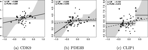
Figure 3: Association between DNA and mRNA for different genes in the breast cancer data set [Neve et al. (2006)]. Segmented copy number is on the x-axis, while gene expression is on the y-axis. Symbols indicate the different states, namely, loss ($\bigtriangledown$), normal ($\bigcirc$) and gain ($\bigtriangleup$). Grey surfaces correspond to 95% uniform CBs. The top left values correspond to $q$-values of tests LM and PLRS, respectively. The dashed line gives the fitted LM model; the “continuous” spline is the fitted PLRS model.

Table 4 gives the number of associations with a $q$-value below 0.1 [based on the Benjamini and Hochberg (1995) FDR]. The LM test is seen to detect slightly more associations as being significant than the PLRS test. This may be a consequence of the fact that the linear model involves fewer parameters. However, closer inspection shows that the sets of detected genes are not nested, and the PLRS test is able to detect biologically meaningful genes that are not detected by the LM test. To illustrate, three DNA-mRNA relationships are plotted in Figure 3. The first corresponds to an association detected as significant with the LM test, but not with the PLRS test. Reciprocally, the last two associations (genes PDE3B and CLIP1) are detected with the PLRS test but not with the LM test. The figure shows that the PLRS test is able to detect relationships for which an effect is present for only a few samples (but at least five). Identifying the last two genes may be more important than the first, as they are more interesting potential targets for studying individual effects.

The first gene in Figure 3 also illustrates that the testing procedures may differ considerably in $q$-values, even though the estimated regression function found by the two models is the same. This is partly explained by the difference in complexity between the alternative models. However, we note that $q$-values for a single gene are not directly comparable, since they also depend on $p$-values of other genes. In Appendix A, we provide, for selected genes, $p$- and $q$-values for the different types of tests.

4.3 Results for selected genes

In this section we show the estimated relationships for selected genes. The selection is based on the Cancer Gene Census list (available at www.sanger.ac.uk/genetics/CGP/Census/) and on our observation that some associations are atypical. Also, we show results for genes C20orf24, TCFL5 and TH1L, which were reported in Carvalho et al. (2009) as important for colorectal cancer progression.

Figures 4 and 5 show nine DNA-mRNA associations for each of the two data sets. Each plot displays the fit of the linear model and of the PLRS model chosen by the OSAIC criterion. Uniform 95% confidence bands (that account for model selection uncertainty) are also plotted. (Some curious shapes result from the fact that pointwise variation bursts near the boundaries and around knots.)

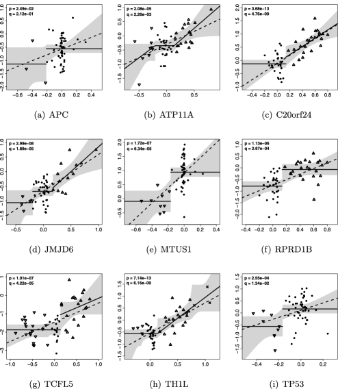
Figure 4: Association between DNA and mRNA for different genes in the colorectal cancer data set. Segmented copy number is on the x-axis, while gene expression is on the y-axis. States are indicated by different symbols: loss ($\bigtriangledown$), normal ($\bigcirc$), gain ($\bigtriangleup$) and amplification ($\times$). Grey surfaces correspond to 95% uniform CBs. In all cases the piecewise linear model is preferred to the simple linear one (dashed line). The top left values correspond to the $p$- and $q$-values of the PLRS test.

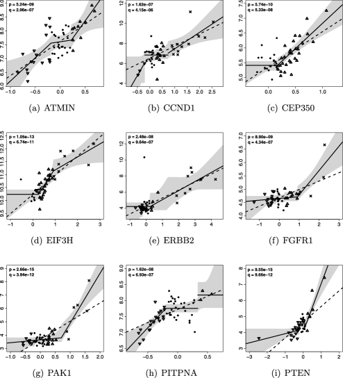
Figure 5: Association between DNA and mRNA for different genes in the breast cancer data set. Segmented copy number is on the x-axis, while gene expression is on the y-axis. States are indicated by different symbols: loss ($\bigtriangledown$), normal ($\bigcirc$), gain ($\bigtriangleup$) and amplification ($\times$). Grey surfaces correspond to 95% uniform CBs. In all cases the piecewise linear model is preferred to the simple linear one (dashed line). The top left values correspond to the $p$- and $q$-values of the PLRS test.

Both figures show a diverse set of forms of associations. Fitted models with jumps reveal that discrete copy number states can, by themselves, explain variation in expression. This is even more true when a piecewise level relationship is identified (as for genes APC and MTUS1 in Figure 4). More generally, piecewise linear models capture effects that differ for losses, gains and/or amplifications. Statistically speaking, this has the advantage of giving more accurate estimates of slope(s), as is clearly observed for genes ATMIN, PITPNA and PTEN in Figure 5. Having a better estimator, we may expect a better test. From a biological point of view, the ability to distinguish effects between states may help the detection of onco and tumor-suppressor genes. Moreover, genes for which these effects concern only a few samples may also be interesting to biologists for studying individual effects.

The simple linear model is observed to be a tight template for modeling. As a matter of fact, it is potentially misleading when the relationship really depends on the underlying copy number state. This happens to be the case for known cancer genes (see FGFR1, PAK1 and PTEN in Figure 5). As a result, when testing the effect of DNA on mRNA with the LM and PLRS tests (see Section 4.2), one may obtain a considerable difference between the $p$-values, and hence $q$-values (see Appendix A). For this reason the proposed framework may improve the detection of (highly) significant associations and their ranking.

Finally, we dwell on the notion of effect in itself. The notion of “association” is broad, and can be expressed both by an intercept and a slope. This can imply a clear difference in interpretation with respect to the linear model. Consider the simple example of gene MTUS1 in Figure 4, where a piecewise level model is preferable. Here intuition clearly tells us that one is more interested in assessing the difference in expression level between samples presenting loss and normal aberrations than an overall trend. Therefore, a linear model may focus on the wrong quantity of interest, whereas the PLRS procedure may yield meaningful interpretation.

We concentrated on comparing our results with those of the linear model. However, it is clear from Figures 4 and 5 that also the other alternative, the piecewise level model (which allows only horizontal lines per state), is often not adequate (see TH1L and PITPNA).

5 Conclusion

We proposed a statistical framework for the integrative analysis of DNA copy number and mRNA expression, which incorporates segmented and called aCGH data. By using discrete aCGH data we improved model flexibility and interpretability. The form of the relationship is allowed to vary per gene. Model interpretation is ameliorated with biologically motivated constraints on the parameters. This complicates the statistical procedures for identifying and inferring the relationship between the markers, but we provided methods for model selection, interval estimation and testing the strength of the association. We applied the methodology to two real data sets. Many (reported) genes exhibited interesting behavior.

A novelty of this work is the combined use of segmented and called aCGH data. Which of the two data types is more suitable is a matter of debate in the aCGH community, and may depend on the type of downstream analysis [van Wieringen, van de Wiel and Ylstra (2007)]. Our method provides a compromise that uses both characteristics of the data.

The form of association between copy number and expression in breast cancer is also explored in the recent paper Solvang et al. (2011) (which we received after completion of this paper). This interesting paper distinguishes (only) between linear and quadratic types of effect and uses (only) two types of aberrations, without distinguishing gains from amplifications. The interpretation of the coefficients in our model seems to be simpler.

The proposed methodology is also applicable to the joint analysis of copy number and microRNA expression. This class of noncoding RNA was shown to play an important role in tumor development. Our method may be particularly suitable for these data, because microRNA transcripts are often expressed in part of the samples only.

Next generation sequencing data will impose new challenges, which will be taken up in future work. This type of data provides higher resolution than microarrays, while reducing biases, in particular, at the lower end of the spectrum. Because expression levels are measured as counts rather than intensities, the distribution of the response variable cannot be assumed to be Gaussian and, hence, a different noise model is needed.

In short, we provide methodology for statistical inference and model selection in the framework of constrained PLRS, and show that this is able to reveal interesting DNA-mRNA relationships for cancer genes. The method is implemented in R and available as a package from www.few.vu.nl/~mavdwiel/ software.html.

Appendix A Testing

See Table 5.

Table 5: $p$ and $q$-values of the test when under the alternative hypothesis H_a the linear, OSAIC-selected and the full models are successively considered. The top and bottom parts correspond, respectively, to the selected genes from the colorectal and breast data

	Linear		OSAIC00.		Full
	$\bolds{p}$	$\bolds{q}$	$\bolds{p}\phantom{00.}$	$\bolds{q}\phantom{00.}$	$\bolds{p}$	$\bolds{q}$
APC	2.49e-02	2.04e-01	2.26e-02	6.38e-02	2.49e-02	2.12e-01
ATP11A	7.34e-06	9.79e-04	5.88e-06	2.98e-04	2.08e-05	2.26e-03
C20orf24	1.71e-12	2.21e-08	3.06e-13	1.14e-09	3.68e-13	4.76e-09
JMJD6	5.44e-09	4.85e-06	1.78e-08	4.31e-06	2.99e-08	1.89e-05
MTUS1	6.83e-07	1.77e-04	6.38e-08	1.06e-05	1.72e-07	6.34e-05
RPRD1B	3.18e-06	5.45e-04	5.17e-07	5.02e-05	1.13e-06	2.67e-04
TCFL5	6.49e-06	8.88e-04	1.75e-08	4.31e-06	1.01e-07	4.22e-05
TH1L	1.06e-10	3.25e-07	2.72e-13	1.14e-09	7.14e-13	6.16e-09
TP53	6.54e-03	9.87e-02	9.42e-05	2.25e-03	2.55e-04	1.34e-02
ATMIN	1.12e-09	6.45e-08	1.13e-09	4.56e-08	5.24e-09	2.96e-07
CCND1	1.91e-08	5.71e-07	3.56e-08	6.88e-07	1.62e-07	4.15e-06
CEP350	8.55e-08	1.93e-06	3.07e-10	1.69e-08	5.74e-10	5.33e-08
EIF3H	1.70e-12	4.88e-10	8.22e-15	3.75e-12	1.05e-13	6.74e-11
ERBB2	4.46e-10	3.18e-08	4.34e-10	2.15e-08	2.48e-08	9.64e-07
FGFR1	1.62e-06	2.03e-05	3.99e-10	2.02e-08	8.90e-09	4.34e-07
PAK1	1.15e-10	1.21e-08	$<$2.2e-1600.	$<$2.2e-1600.	2.66e-15	3.94e-12
PITPNA	1.85e-06	2.25e-05	8.40e-10	3.66e-08	1.62e-08	6.93e-07
PTEN	7.27e-09	2.64e-07	9.10e-15	4.02e-12	9.55e-15	9.66e-12

Appendix B Semidefinite programming

Here, we provide the two equivalence relationships from Vandenberghe and Boyd (1996) that are necessary to express the semidefinite program. We recall that a linear matrix inequality (LMI) type of constraint includes, among others, linear and convex quadratic inequalities. These are the two types of constraints we are interested in. To express them as two LMIs, we make use of the following equivalences.

A linear inequality constraint $Ax+b\geq 0$, where $A=[a_{1}\cdots a_{k}]$ and $x\in\mathbb{R}^{n}$, is equivalent to the following LMI:

$$F(x)=F_{0}+\sum_{i=1}^{k}{x_{i}F_{i}}\succeq 0,$$

where $F_{0}=\operatorname{diag}(b)$, $F_{i}=\operatorname{diag}(a_{i})$, $i=1,\ldots,k$. $\operatorname{diag}(v)$ represents the diagonal matrix with the vector $v$ on its diagonal.

A convex quadratic constraint $(Ax+b)^{T}(Ax+b)-c^{T}x-d\leq 0$, where $A=[a_{1}\cdots a_{k}]$ and $x\in\mathbb{R}^{n}$, is equivalent to the following LMI:

$$F(x)=F_{0}+\sum_{i=1}^{k}{x_{i}F_{i}}\succeq 0,$$

where

$$F_{0}=\pmatrix{I&b\vspace*{2pt}\cr b^{T}&d},\qquad F_{i}=\pmatrix{0&a_{i}\vspace*{2pt}\cr a_{i}^{T}&c_{i}},\qquad i=1,\ldots,k.$$

Multiple LMIs can be expressed as a single one using block diagonal matrices [VanAntwerp (2000)].

References

- Akaike (1973) {bincollection}[mr] \bauthor\bsnmAkaike, \bfnmH.\binitsH. (\byear1973). \btitleInformation theory and an extension of the maximum likelihood principle. In \bbooktitleSecond International Symposium on Information Theory (Tsahkadsor, 1971) (\beditor\bfnmB. N.\binitsB. N. \bsnmPetrov and \beditor\bfnmF.\binitsF. \bsnmCsaki, eds.) \bpages267–281. \bpublisherAkadémiai Kiadó, \blocationBudapest. \bidmr=0483125 \bptokimsref \endbibitem
- Andrews (2000) {barticle}[mr] \bauthor\bsnmAndrews, \bfnmDonald W. K.\binitsD. W. K. (\byear2000). \btitleInconsistency of the bootstrap when a parameter is on the boundary of the parameter space. \bjournalEconometrica \bvolume68 \bpages399–405. \biddoi=10.1111/1468-0262.00114, issn=0012-9682, mr=1748009 \bptokimsref \endbibitem
- Arnold and Shavelle (1998) {barticle}[mr] \bauthor\bsnmArnold, \bfnmBarry C.\binitsB. C. and \bauthor\bsnmShavelle, \bfnmRobert M.\binitsR. M. (\byear1998). \btitleJoint confidence sets for the mean and variance of a normal distribution. \bjournalAmer. Statist. \bvolume52 \bpages133–140. \biddoi=10.2307/2685471, issn=0003-1305, mr=1628439 \bptokimsref \endbibitem
- Asimit, Andrulis and Bull (2011) {barticle}[mr] \bauthor\bsnmAsimit, \bfnmJennifer L.\binitsJ. L., \bauthor\bsnmAndrulis, \bfnmIrene L.\binitsI. L. and \bauthor\bsnmBull, \bfnmShelley B.\binitsS. B. (\byear2011). \btitleRegression models, scan statistics and reappearance probabilities to detect regions of association between gene expression and copy number. \bjournalStat. Med. \bvolume30 \bpages1157–1178. \biddoi=10.1002/sim.4193, issn=0277-6715, mr=2767848 \bptokimsref \endbibitem
- Benjamini and Hochberg (1995) {barticle}[mr] \bauthor\bsnmBenjamini, \bfnmYoav\binitsY. and \bauthor\bsnmHochberg, \bfnmYosef\binitsY. (\byear1995). \btitleControlling the false discovery rate: A practical and powerful approach to multiple testing. \bjournalJ. Roy. Statist. Soc. Ser. B \bvolume57 \bpages289–300. \bidissn=0035-9246, mr=1325392 \bptokimsref \endbibitem
- Bicciato et al. (2009) {barticle}[pbm] \bauthor\bsnmBicciato, \bfnmSilvio\binitsS., \bauthor\bsnmSpinelli, \bfnmRoberta\binitsR., \bauthor\bsnmZampieri, \bfnmMattia\binitsM., \bauthor\bsnmMangano, \bfnmEleonora\binitsE., \bauthor\bsnmFerrari, \bfnmFrancesco\binitsF., \bauthor\bsnmBeltrame, \bfnmLuca\binitsL., \bauthor\bsnmCifola, \bfnmIngrid\binitsI., \bauthor\bsnmPeano, \bfnmClelia\binitsC., \bauthor\bsnmSolari, \bfnmAldo\binitsA. and \bauthor\bsnmBattaglia, \bfnmCristina\binitsC. (\byear2009). \btitleA computational procedure to identify significant overlap of differentially expressed and genomic imbalanced regions in cancer datasets. \bjournalNucleic Acids Res. \bvolume37 \bpages5057–5070. \biddoi=10.1093/nar/gkp520, issn=1362-4962, pii=gkp520, pmcid=2731905, pmid=19542187 \bptokimsref \endbibitem
- Boyd and Vandenberghe (2004) {bbook}[mr] \bauthor\bsnmBoyd, \bfnmStephen\binitsS. and \bauthor\bsnmVandenberghe, \bfnmLieven\binitsL. (\byear2004). \btitleConvex Optimization. \bpublisherCambridge Univ. Press, \blocationCambridge. \bidmr=2061575 \bptokimsref \endbibitem
- Bozdogan (1987) {barticle}[mr] \bauthor\bsnmBozdogan, \bfnmHamparsum\binitsH. (\byear1987). \btitleModel selection and Akaike’s information criterion (AIC): The general theory and its analytical extensions. \bjournalPsychometrika \bvolume52 \bpages345–370. \biddoi=10.1007/BF02294361, issn=0033-3123, mr=0914460 \bptokimsref \endbibitem
- Brown, Cai and DasGupta (2003) {barticle}[mr] \bauthor\bsnmBrown, \bfnmLawrence D.\binitsL. D., \bauthor\bsnmCai, \bfnmT. Tony\binitsT. T. and \bauthor\bsnmDasGupta, \bfnmAnirban\binitsA. (\byear2003). \btitleInterval estimation in exponential families. \bjournalStatist. Sinica \bvolume13 \bpages19–49. \bidissn=1017-0405, mr=1963918 \bptokimsref \endbibitem
- Buckland, Burnham and Augustin (1997) {barticle}[author] \bauthor\bsnmBuckland, \bfnmS. T.\binitsS. T., \bauthor\bsnmBurnham, \bfnmK. P.\binitsK. P. and \bauthor\bsnmAugustin, \bfnmN. H.\binitsN. H. (\byear1997). \btitleModel selection: An integral part of inference. \bjournalBiometrics \bvolume53 \bpages603–618. \bptokimsref \endbibitem
- Burnham and Anderson (2002) {bbook}[mr] \bauthor\bsnmBurnham, \bfnmKenneth P.\binitsK. P. and \bauthor\bsnmAnderson, \bfnmDavid R.\binitsD. R. (\byear2002). \btitleModel Selection and Multimodel Inference: A Practical Information-Theoretic Approach, \bedition2nd ed. \bpublisherSpringer, \blocationNew York. \bidmr=1919620 \bptokimsref \endbibitem
- Carvalho et al. (2009) {barticle}[pbm] \bauthor\bsnmCarvalho, \bfnmB.\binitsB., \bauthor\bsnmPostma, \bfnmC.\binitsC., \bauthor\bsnmMongera, \bfnmS.\binitsS., \bauthor\bsnmHopmans, \bfnmE.\binitsE., \bauthor\bsnmDiskin, \bfnmS.\binitsS., \bauthor\bparticlevan de \bsnmWiel, \bfnmM. A.\binitsM. A., \bauthor\bparticlevan \bsnmCriekinge, \bfnmW.\binitsW., \bauthor\bsnmThas, \bfnmO.\binitsO., \bauthor\bsnmMatthäi, \bfnmA.\binitsA., \bauthor\bsnmCuesta, \bfnmM. A.\binitsM. A., \bauthor\bsnmDroste, \bfnmJ. S. Terhaar Sive\binitsJ. S. T. S., \bauthor\bsnmCraanen, \bfnmM.\binitsM., \bauthor\bsnmSchröck, \bfnmE.\binitsE., \bauthor\bsnmYlstra, \bfnmB.\binitsB. and \bauthor\bsnmMeijer, \bfnmG. A.\binitsG. A. (\byear2009). \btitleMultiple putative oncogenes at the chromosome 20q amplicon contribute to colorectal adenoma to carcinoma progression. \bjournalGut \bvolume58 \bpages79–89. \biddoi=10.1136/gut.2007.143065, issn=1468-3288, pii=gut.2007.143065, pmid=18829976 \bptokimsref \endbibitem
- Chernoff (1954) {barticle}[mr] \bauthor\bsnmChernoff, \bfnmHerman\binitsH. (\byear1954). \btitleOn the distribution of the likelihood ratio. \bjournalAnn. Math. Statistics \bvolume25 \bpages573–578. \bidissn=0003-4851, mr=0065087 \bptokimsref \endbibitem
- Gouriéroux, Holly and Monfort (1982) {barticle}[mr] \bauthor\bsnmGouriéroux, \bfnmChristian\binitsC., \bauthor\bsnmHolly, \bfnmAlberto\binitsA. and \bauthor\bsnmMonfort, \bfnmAlain\binitsA. (\byear1982). \btitleLikelihood ratio test, Wald test, and Kuhn–Tucker test in linear models with inequality constraints on the regression parameters. \bjournalEconometrica \bvolume50 \bpages63–80. \biddoi=10.2307/1912529, issn=0012-9682, mr=0640166 \bptokimsref \endbibitem
- Grömping (2010) {barticle}[author] \bauthor\bsnmGrömping, \bfnmUlrike\binitsU. (\byear2010). \btitleInference with linear equality and inequality constraints using R: The package ic.infer. \bjournalJ. Stat. Softw. \bvolume33 \bpages1–31. \bptokimsref \endbibitem
- Gu, Choi and Ghosh (2008) {barticle}[pbm] \bauthor\bsnmGu, \bfnmWenjuan\binitsW., \bauthor\bsnmChoi, \bfnmHyungwon\binitsH. and \bauthor\bsnmGhosh, \bfnmDebashis\binitsD. (\byear2008). \btitleGlobal associations between copy number and transcript mRNA microarray data: An empirical study. \bjournalCancer Inform. \bvolume6 \bpages17–23. \bidissn=1176-9351, pmcid=2623285, pmid=19259399 \bptokimsref \endbibitem
- Hughes and King (2003) {barticle}[mr] \bauthor\bsnmHughes, \bfnmAnthony W.\binitsA. W. and \bauthor\bsnmKing, \bfnmMaxwell L.\binitsM. L. (\byear2003). \btitleModel selection using AIC in the presence of one-sided information. \bjournalJ. Statist. Plann. Inference \bvolume115 \bpages397–411. \biddoi=10.1016/S0378-3758(02)00159-3, issn=0378-3758, mr=1985874 \bptokimsref \endbibitem
- Jörnsten et al. (2011) {barticle}[pbm] \bauthor\bsnmJörnsten, \bfnmRebecka\binitsR., \bauthor\bsnmAbenius, \bfnmTobias\binitsT., \bauthor\bsnmKling, \bfnmTeresia\binitsT., \bauthor\bsnmSchmidt, \bfnmLinnéa\binitsL., \bauthor\bsnmJohansson, \bfnmErik\binitsE., \bauthor\bsnmNordling, \bfnmTorbjörn E. M.\binitsT. E. M., \bauthor\bsnmNordlander, \bfnmBodil\binitsB., \bauthor\bsnmSander, \bfnmChris\binitsC., \bauthor\bsnmGennemark, \bfnmPeter\binitsP., \bauthor\bsnmFuna, \bfnmKeiko\binitsK., \bauthor\bsnmNilsson, \bfnmBjörn\binitsB., \bauthor\bsnmLindahl, \bfnmLinda\binitsL. and \bauthor\bsnmNelander, \bfnmSven\binitsS. (\byear2011). \btitleNetwork modeling of the transcriptional effects of copy number aberrations in glioblastoma. \bjournalMol. Syst. Biol. \bvolume7 \bpages486. \biddoi=10.1038/msb.2011.17, issn=1744-4292, pii=msb201117, pmcid=3101951, pmid=21525872 \bptokimsref \endbibitem
- Kodde and Palm (1986) {barticle}[mr] \bauthor\bsnmKodde, \bfnmDavid A.\binitsD. A. and \bauthor\bsnmPalm, \bfnmFranz C.\binitsF. C. (\byear1986). \btitleWald criteria for jointly testing equality and inequality restrictions. \bjournalEconometrica \bvolume54 \bpages1243–1248. \biddoi=10.2307/1912331, issn=0012-9682, mr=0859464 \bptokimsref \endbibitem
- Kudô (1963) {barticle}[mr] \bauthor\bsnmKudô, \bfnmAkio\binitsA. (\byear1963). \btitleA multivariate analogue of the one-sided test. \bjournalBiometrika \bvolume50 \bpages403–418. \bidissn=0006-3444, mr=0163386 \bptokimsref \endbibitem
- Leday et al. (2013) {bmisc}[author] \bauthor\bsnmLeday, \bfnmGwenaël G. R.\binitsG. G. R., \bauthor\bparticlevan der \bsnmVaart, \bfnmAad W.\binitsA. W., \bauthor\bparticlevan \bsnmWieringen, \bfnmWessel N.\binitsW. N. and \bauthor\bparticlevan de \bsnmWiel, \bfnmMark A.\binitsM. A. (\byear2013). \bhowpublishedSupplement to “Modeling association between DNA copy number and gene expression with constrained piecewise linear regression splines.” DOI:\doiurl10.1214/12-AOAS605SUPP. \bptokimsref \endbibitem
- Lee, Kong and Park (2008) {barticle}[author] \bauthor\bsnmLee, \bfnmHyunju\binitsH., \bauthor\bsnmKong, \bfnmSek W.\binitsS. W. and \bauthor\bsnmPark, \bfnmPeter J.\binitsP. J. (\byear2008). \btitleIntegrative analysis reveals the direct and indirect interactions between DNA copy number aberrations and gene expression changes. \bjournalBioinformatics \bvolume24 \bpages889–896. \bptokimsref \endbibitem
- Lipson et al. (2004) {bincollection}[mr] \bauthor\bsnmLipson, \bfnmDoron\binitsD., \bauthor\bsnmBen-Dor, \bfnmAmir\binitsA., \bauthor\bsnmDehan, \bfnmElinor\binitsE. and \bauthor\bsnmYakhini, \bfnmZohar\binitsZ. (\byear2004). \btitleJoint analysis of DNA copy numbers and gene expression levels. In \bbooktitleAlgorithms in Bioinformatics. \bseriesLecture Notes in Computer Science \bvolume3240 \bpages135–146. \bpublisherSpringer, \blocationBerlin. \biddoi=10.1007/978-3-540-30219-3_12, mr=2155600 \bptokimsref \endbibitem
- Meeker and Escobar (1995) {barticle}[author] \bauthor\bsnmMeeker, \bfnmWilliam Q.\binitsW. Q. and \bauthor\bsnmEscobar, \bfnmLuis A.\binitsL. A. (\byear1995). \btitleTeaching about approximate confidence regions based on maximum likelihood estimation. \bjournalAmer. Statist. \bvolume49 \bpages48–53. \bptokimsref \endbibitem
- Menezes et al. (2009) {barticle}[author] \bauthor\bsnmMenezes, \bfnmRenee\binitsR., \bauthor\bsnmBoetzer, \bfnmMarten\binitsM., \bauthor\bsnmSieswerda, \bfnmMelle\binitsM., \bauthor\bparticlevan \bsnmOmmen, \bfnmGert J.\binitsG. J. and \bauthor\bsnmBoer, \bfnmJudith\binitsJ. (\byear2009). \btitleIntegrated analysis of DNA copy number and gene expression microarray data using gene sets. \bjournalBMC Bioinformatics \bvolume10 \bpages203+. \bptokimsref \endbibitem
- Neve et al. (2006) {barticle}[author] \bauthor\bsnmNeve, \bfnmRichard M.\binitsR. M., \bauthor\bsnmChin, \bfnmKoei\binitsK., \bauthor\bsnmFridlyand, \bfnmJane\binitsJ., \bauthor\bsnmYeh, \bfnmJennifer\binitsJ., \bauthor\bsnmBaehner, \bfnmFrederick L.\binitsF. L., \bauthor\bsnmFevr, \bfnmTea\binitsT., \bauthor\bsnmClark, \bfnmLaura\binitsL., \bauthor\bsnmBayani, \bfnmNora\binitsN., \bauthor\bsnmCoppe, \bfnmJean-Philippe P.\binitsJ.-P. P., \bauthor\bsnmTong, \bfnmFrances\binitsF., \bauthor\bsnmSpeed, \bfnmTerry\binitsT., \bauthor\bsnmSpellman, \bfnmPaul T.\binitsP. T., \bauthor\bsnmDeVries, \bfnmSandy\binitsS., \bauthor\bsnmLapuk, \bfnmAnna\binitsA., \bauthor\bsnmWang, \bfnmNick J.\binitsN. J., \bauthor\bsnmKuo, \bfnmWen-Lin L.\binitsW.-L. L., \bauthor\bsnmStilwell, \bfnmJackie L.\binitsJ. L., \bauthor\bsnmPinkel, \bfnmDaniel\binitsD., \bauthor\bsnmAlbertson, \bfnmDonna G.\binitsD. G., \bauthor\bsnmWaldman, \bfnmFrederic M.\binitsF. M., \bauthor\bsnmMcCormick, \bfnmFrank\binitsF., \bauthor\bsnmDickson, \bfnmRobert B.\binitsR. B., \bauthor\bsnmJohnson, \bfnmMichael D.\binitsM. D., \bauthor\bsnmLippman, \bfnmMarc\binitsM., \bauthor\bsnmEthier, \bfnmStephen\binitsS., \bauthor\bsnmGazdar, \bfnmAdi\binitsA. and \bauthor\bsnmGray, \bfnmJoe W.\binitsJ. W. (\byear2006). \btitleA collection of breast cancer cell lines for the study of functionally distinct cancer subtypes. \bjournalCancer Cell. \bvolume10 \bpages515–527. \bptokimsref \endbibitem
- Olshen et al. (2004) {barticle}[pbm] \bauthor\bsnmOlshen, \bfnmAdam B.\binitsA. B., \bauthor\bsnmVenkatraman, \bfnmE. S.\binitsE. S., \bauthor\bsnmLucito, \bfnmRobert\binitsR. and \bauthor\bsnmWigler, \bfnmMichael\binitsM. (\byear2004). \btitleCircular binary segmentation for the analysis of array-based DNA copy number data. \bjournalBiostatistics \bvolume5 \bpages557–572. \biddoi=10.1093/biostatistics/kxh008, issn=1465-4644, pii=5/4/557, pmid=15475419 \bptokimsref \endbibitem
- Peng et al. (2010) {barticle}[mr] \bauthor\bsnmPeng, \bfnmJie\binitsJ., \bauthor\bsnmZhu, \bfnmJi\binitsJ., \bauthor\bsnmBergamaschi, \bfnmAnna\binitsA., \bauthor\bsnmHan, \bfnmWonshik\binitsW., \bauthor\bsnmNoh, \bfnmDong-Young\binitsD.-Y., \bauthor\bsnmPollack, \bfnmJonathan R.\binitsJ. R. and \bauthor\bsnmWang, \bfnmPei\binitsP. (\byear2010). \btitleRegularized multivariate regression for identifying master predictors with application to integrative genomics study of breast cancer. \bjournalAnn. Appl. Stat. \bvolume4 \bpages53–77. \biddoi=10.1214/09-AOAS271, issn=1932-6157, mr=2758084 \bptokimsref \endbibitem
- Pinkel and Albertson (2005) {barticle}[pbm] \bauthor\bsnmPinkel, \bfnmDaniel\binitsD. and \bauthor\bsnmAlbertson, \bfnmDonna G.\binitsD. G. (\byear2005). \btitleArray comparative genomic hybridization and its applications in cancer. \bjournalNat. Genet. \bvolume37 Suppl. \bpagesS11–S17. \biddoi=10.1038/ng1569, issn=1061-4036, pii=ng1569, pmid=15920524 \bptokimsref \endbibitem
- Quackenbush (2002) {barticle}[pbm] \bauthor\bsnmQuackenbush, \bfnmJohn\binitsJ. (\byear2002). \btitleMicroarray data normalization and transformation. \bjournalNat. Genet. \bvolume32 Suppl. \bpages496–501. \biddoi=10.1038/ng1032, issn=1061-4036, pii=ng1032, pmid=12454644 \bptokimsref \endbibitem
- Robertson, Wright and Dykstra (1988) {bbook}[mr] \bauthor\bsnmRobertson, \bfnmTim\binitsT., \bauthor\bsnmWright, \bfnmF. T.\binitsF. T. and \bauthor\bsnmDykstra, \bfnmR. L.\binitsR. L. (\byear1988). \btitleOrder Restricted Statistical Inference. \bpublisherWiley, \blocationChichester. \bidmr=0961262 \bptokimsref \endbibitem
- Salari, Tibshirani and Pollack (2010) {barticle}[pbm] \bauthor\bsnmSalari, \bfnmKeyan\binitsK., \bauthor\bsnmTibshirani, \bfnmRobert\binitsR. and \bauthor\bsnmPollack, \bfnmJonathan R.\binitsJ. R. (\byear2010). \btitleDR-Integrator: A new analytic tool for integrating DNA copy number and gene expression data. \bjournalBioinformatics \bvolume26 \bpages414–416. \biddoi=10.1093/bioinformatics/btp702, issn=1367-4811, pii=btp702, pmcid=2815664, pmid=20031972 \bptokimsref \endbibitem
- Schäfer et al. (2009) {barticle}[pbm] \bauthor\bsnmSchäfer, \bfnmMartin\binitsM., \bauthor\bsnmSchwender, \bfnmHolger\binitsH., \bauthor\bsnmMerk, \bfnmSylvia\binitsS., \bauthor\bsnmHaferlach, \bfnmClaudia\binitsC., \bauthor\bsnmIckstadt, \bfnmKatja\binitsK. and \bauthor\bsnmDugas, \bfnmMartin\binitsM. (\byear2009). \btitleIntegrated analysis of copy number alterations and gene expression: A bivariate assessment of equally directed abnormalities. \bjournalBioinformatics \bvolume25 \bpages3228–3235. \biddoi=10.1093/bioinformatics/btp592, issn=1367-4811, pii=btp592, pmid=19828576 \bptokimsref \endbibitem
- Shapiro (1988) {barticle}[mr] \bauthor\bsnmShapiro, \bfnmA.\binitsA. (\byear1988). \btitleTowards a unified theory of inequality constrained testing in multivariate analysis. \bjournalInternat. Statist. Rev. \bvolume56 \bpages49–62. \biddoi=10.2307/1403361, issn=0306-7734, mr=0963140 \bptokimsref \endbibitem
- Silvapulle and Sen (2005) {bbook}[mr] \bauthor\bsnmSilvapulle, \bfnmMervyn J.\binitsM. J. and \bauthor\bsnmSen, \bfnmPranab K.\binitsP. K. (\byear2005). \btitleConstrained Statistical Inference: Inequality, Order, and Shape Restrictions. \bpublisherWiley, \blocationHoboken, NJ. \bidmr=2099529 \bptnotecheck year\bptokimsref \endbibitem
- Solvang et al. (2011) {barticle}[pbm] \bauthor\bsnmSolvang, \bfnmHiroko K.\binitsH. K., \bauthor\bsnmLingjærde, \bfnmOle Christian\binitsO. C., \bauthor\bsnmFrigessi, \bfnmArnoldo\binitsA., \bauthor\bsnmBørresen-Dale, \bfnmAnne-Lise\binitsA.-L. and \bauthor\bsnmKristensen, \bfnmVessela N.\binitsV. N. (\byear2011). \btitleLinear and non-linear dependencies between copy number aberrations and mRNA expression reveal distinct molecular pathways in breast cancer. \bjournalBMC Bioinformatics \bvolume12 \bpages197. \biddoi=10.1186/1471-2105-12-197, issn=1471-2105, pii=1471-2105-12-197, pmcid=3128865, pmid=21609452 \bptokimsref \endbibitem
- Soneson et al. (2010) {barticle}[pbm] \bauthor\bsnmSoneson, \bfnmCharlotte\binitsC., \bauthor\bsnmLilljebjörn, \bfnmHenrik\binitsH., \bauthor\bsnmFioretos, \bfnmThoas\binitsT. and \bauthor\bsnmFontes, \bfnmMagnus\binitsM. (\byear2010). \btitleIntegrative analysis of gene expression and copy number alterations using canonical correlation analysis. \bjournalBMC Bioinformatics \bvolume11 \bpages191. \biddoi=10.1186/1471-2105-11-191, issn=1471-2105, pii=1471-2105-11-191, pmcid=2873536, pmid=20398334 \bptokimsref \endbibitem
- van de Wiel et al. (2007) {barticle}[author] \bauthor\bparticlevan de \bsnmWiel, \bfnmMark A.\binitsM. A., \bauthor\bsnmKim, \bfnmKyung I.\binitsK. I., \bauthor\bsnmVosse, \bfnmSjoerd J.\binitsS. J., \bauthor\bparticlevan \bsnmWieringen, \bfnmWessel N.\binitsW. N., \bauthor\bsnmWilting, \bfnmSaskia M.\binitsS. M. and \bauthor\bsnmYlstra, \bfnmBauke\binitsB. (\byear2007). \btitleCGHcall: Calling aberrations for array CGH tumor profiles. \bjournalBioinformatics \bvolume23 \bpages892–894. \bptokimsref \endbibitem
- van de Wiel et al. (2011) {barticle}[pbm] \bauthor\bparticlevan de \bsnmWiel, \bfnmMark A.\binitsM. A., \bauthor\bsnmPicard, \bfnmFranck\binitsF., \bauthor\bparticlevan \bsnmWieringen, \bfnmWessel N.\binitsW. N. and \bauthor\bsnmYlstra, \bfnmBauke\binitsB. (\byear2011). \btitlePreprocessing and downstream analysis of microarray DNA copy number profiles. \bjournalBrief. Bioinformatics \bvolume12 \bpages10–21. \biddoi=10.1093/bib/bbq004, issn=1477-4054, pii=bbq004, pmid=20172948 \bptnotecheck year\bptokimsref \endbibitem
- van der Vaart (1998) {bbook}[mr] \bauthor\bparticlevan der \bsnmVaart, \bfnmA. W.\binitsA. W. (\byear1998). \btitleAsymptotic Statistics. \bseriesCambridge Series in Statistical and Probabilistic Mathematics \bvolume3. \bpublisherCambridge Univ. Press, \blocationCambridge. \bidmr=1652247 \bptokimsref \endbibitem
- van Wieringen, Berkhof and van de Wiel (2010) {barticle}[mr] \bauthor\bparticlevan \bsnmWieringen, \bfnmWessel N.\binitsW. N., \bauthor\bsnmBerkhof, \bfnmJohannes\binitsJ. and \bauthor\bparticlevan de \bsnmWiel, \bfnmMark A.\binitsM. A. (\byear2010). \btitleA random coefficients model for regional co-expression associated with DNA copy number. \bjournalStat. Appl. Genet. Mol. Biol. \bvolume9 \bpages30. \biddoi=10.2202/1544-6115.1531, issn=1544-6115, mr=2721705 \bptokimsref \endbibitem
- van Wieringen, van de Wiel and Ylstra (2007) {barticle}[author] \bauthor\bparticlevan \bsnmWieringen, \bfnmWessel N.\binitsW. N., \bauthor\bparticlevan de \bsnmWiel, \bfnmMark A.\binitsM. A. and \bauthor\bsnmYlstra, \bfnmBauke\binitsB. (\byear2007). \btitleNormalized, segmented or called aCGH data? \bjournalCancer Inform. \bvolume3 \bpages321–327. \bptokimsref \endbibitem
- van Wieringen and van de Wiel (2009) {barticle}[mr] \bauthor\bparticlevan \bsnmWieringen, \bfnmWessel N.\binitsW. N. and \bauthor\bparticlevan de \bsnmWiel, \bfnmMark A.\binitsM. A. (\byear2009). \btitleNonparametric testing for DNA copy number induced differential mRNA gene expression. \bjournalBiometrics \bvolume65 \bpages19–29. \biddoi=10.1111/j.1541-0420.2008.01052.x, issn=0006-341X, mr=2665842 \bptokimsref \endbibitem
- VanAntwerp (2000) {barticle}[author] \bauthor\bsnmVanAntwerp, \bfnmJ.\binitsJ. (\byear2000). \btitleA tutorial on linear and bilinear matrix inequalities. \bjournalJ. Process Contr. \bvolume10 \bpages363–385. \bptokimsref \endbibitem
- Vandenberghe and Boyd (1996) {barticle}[mr] \bauthor\bsnmVandenberghe, \bfnmLieven\binitsL. and \bauthor\bsnmBoyd, \bfnmStephen\binitsS. (\byear1996). \btitleSemidefinite programming. \bjournalSIAM Rev. \bvolume38 \bpages49–95. \biddoi=10.1137/1038003, issn=0036-1445, mr=1379041 \bptokimsref \endbibitem