Vacuum structure in $3d$ supersymmetric gauge theories

A. V. Smilga

SUBATECH, Université de Nantes,

4 rue Alfred Kastler, BP 20722, Nantes 44307, France

E-mail: smilga@subatech.in2p3.fr

Based on a talk given at the Pomeranchuk memorial conference in ITEP in June 2013, we review the vacuum dynamics in $3d$ supersymmetric Yang-Mills-Chern-Simons theories with and without extra matter multiplets. By analyzing the effective Born-Oppenheimer Hamiltonian in a small spatial box, we calculate the number of vacuum states (the Witten index) and examine their structure for these theories. The results are identical to those obtained by other methods.

1 Introduction

Probably, the best known scientific achievement of Isaak Yakovlich Pomeranchuk was the concept of the vacuum Regge pole that is nowadays called the pomeron. I did not have a chance to meet Pomeranchuk personally — I came to ITEP when he was already gone. But I heard many times from his colleagues and collaborators that Isaak Yakovlich atrributed a great significance to studying properties of the vacuum, and even used to joke about an urgent need for the ITEP theory group to buy a powerful pump for that purpose.

Pomeranchuk did not know that, with the advent of supersymmetry, the issues of vacuum structure and vacuum counting would acquire a special interest. The existence of supersymmetric vacua (ground states of the Hamiltonian annihilated by the action of supercharges and having zero energy) shows that supersymmetry is unbroken, while the absence of such states signals spontaneous breaking of supersymmetry. The crucial quantity to be studied in this respect is the Witten index, the difference between the numbers of bosonic and fermionic vacuum states, which also can be represented as

$$I\ =\ {\rm Tr}\{(-1)^{F}e^{-\beta H}\}$$ (1.1)

where $H$ is the Hamiltonian and $F$ is the fermion charge operator. Due to supersymmetry, nonvacuum contributions in the trace cancel. It is important that the quantity (1.1) represents an index, a close relative of the Atiyah-Singer index and other topological invariants, which is invariant under smooth Hamiltonian deformations. The latter circumstance allows one to evaluate the Witten index for rather complicated theories: it is sufficient to find out a proper simplifying deformation.

My talk (based on three recent studies [1, 2, 3] ) is devoted exactly to that. I will study the vacuum dynamics in a particular class of theories — supersymmetric 3-dimensional gauge theories involving the Chern-Simons term. Such theories have recently attracted a considerable attention in view of newly discovered dualities between certain ${\cal N}=8$ and ${\cal N}=6$ versions of these theories and the respective string theories on $AdS_{4}\times S^{7}$ or $AdS_{4}\times\mathbb{C}\mathbb{P}^{3}$ backgrounds [4, 5]. Note, however, that the field theories dual to string theories are conformal and do not involve a mass gap. In such theories, the conventional Witten (alias, toroidal) index we are interested in here is not well defined, and the proper tool to study them is the so called superconformal (alias, spherical) index [9, 10].

We calculate the index by deforming the theory, putting it in a small spatial box and studying the dynamics of the Hamiltonian thus obtained in the framework of the Born–Oppenheimer (BO) approximation. The results coincide with those obtained by other methods.

Let us discuss first the simplest such theory, the ${\cal N}=1$ supersymmetric Yang-Mills-Chern-Simons theory with the Lagrangian

$${\cal L}\ =\ \frac{1}{g^{2}}\left\langle-\frac{1}{2}F_{\mu\nu}^{2}+i\bar{\lambda}/\!\!\!\!D\lambda\right\rangle+\kappa\left\langle\epsilon^{\mu\nu\rho}\left(A_{\mu}\partial_{\nu}A_{\rho}-\frac{2i}{3}A_{\mu}A_{\nu}A_{\rho}\right)-\bar{\lambda}\lambda\right\rangle\,.$$ (1.2)

The conventions are: $\epsilon^{012}=1,\ D_{\mu}{\cal O}=\partial_{\mu}{\cal O}-i[A_{\mu},{\cal O}]$ (such that $A_{\mu}$ is Hermitian), $\lambda_{\alpha}$ is a 2-component Majorana $3d$ spinor belonging to the adjoint representation of the gauge group, and $\langle\ldots\rangle$ stands for the color trace. We choose

$$\gamma^{0}\ =\ \sigma^{2},\ \ \ \gamma^{1}=i\sigma^{1},\ \ \ \gamma^{2}=i\sigma^{3}\ .$$ (1.3)

This is a $3d$ theory and the gauge coupling constant $g^{2}$ carries the dimension of mass. The physical boson and fermion degrees of freedom in this theory are massive,

$$m=\kappa g^{2}\ .$$ (1.4)

In three dimensions, a nonzero mass brings about parity breaking. The requirement for $e^{iS}$ to be invariant under certain large (noncontractible) gauge transformations (see e.g. Ref.[11] for a nice review) leads to the quantization condition

$$\kappa=\frac{k}{4\pi}\ .$$ (1.5)

with integer or sometimes (see below) half-integer level $k$.

The index (1.1) was evaluated in [12] with the result

$$I(k,N)\ =\ [{\rm sgn}(k)]^{N-1}\left(\begin{array}[]{c}|k|+N/2-1\\ N-1\end{array}\right)\ .$$ (1.8)

for $SU(N)$ gauge group. This is valid for $|k|\geq N/2$. For $|k|<N/2$, the index vanishes and supersymmetry is broken. In the simplest $SU(2)$ case, the index is just

$$I(k,2)\ =\ k\ .$$ (1.9)

For $SU(3)$, it is

$$I(k,3)\ =\ \frac{k^{2}-1/4}{2}\,.$$ (1.10)

We can now notice that, for the index to be integer, the level $k$ should be a half-integer rather than an integer for $SU(3)$ and for all unitary groups with odd $N$. The explanation is that in these cases, the large gauge transformation mentioned above not only shifts the classical action, but also contributes the extra factor $(-1)$ due to the modification of the fermion determinant [13, 14].

The result (1.8) was derived in [12] by the following reasoning. Consider the theory in a large spatial volume, $g^{2}L\gg 1$. Consider then the functional integral for the index (1.1) and mentally perform a Gaussian integration over fermionic variables. This gives an effective bosonic action that involves the CS term, the Yang-Mills term and other higher-derivative gauge-invariant terms. After that, the coefficient of the CS term is renormalized ,

$$k\ \to\ k-\frac{N}{2}\,.$$ (1.11)

At large $\beta$, the sum (1.1) is saturated by the vacuum states of the theory and hence depends on the low-energy dynamics of the corresponding effective Hamiltonian. The vacuum states are determined by the term with the lowest number of derivatives, i.e. the Chern-Simons term; the effects due to the YM term and still higher derivative terms are suppressed at small energies and a large spatial volume. Basically, the spectrum of vacuum states coincides with the full spectrum in the topological pure CS theory. The latter was determined some time ago

• by establishing a relationship between the pure $3d$ CS theories and $2d$ WZNW theories [15]

• by canonical quantization of the CS theory and direct determination of the wave functions annihilated by the Gauss law constraints [16, 17].

The index (1.8) is then determined as the number of states in pure CS theory with the shift (1.11). For example, in the $SU(2)$ case, the number of CS states is $k+1$, which gives (1.9) after the shift.

In Sections 2 and 3, we will rederive the result (1.8) using another method. We choose the spatial box to be small rather than large, $g^{2}L\ll 1$, and study the dynamics of the corresponding BO Hamiltonian. This method was developped in [18] and applied there to $4d$ SYM theories. We now explain how it works.

Take the simplest $SU(2)$ theory. With periodic boundary conditions for all fields , the slow variables in the effective BO Hamiltonian are just the zero Fourier modes of the spatial components of the Abelian vector potential and its superpartners,

$$C_{j}\ =\ A_{j}^{({\bf 0})3},\ \ \ \ \ \ \ \ \ \ \lambda_{\alpha}\ =\ \lambda_{\alpha}^{({\bf 0})3}\,.$$ (1.12)

(In the $4d$ case, the spatial index $j$ takes three values, $j=1,2,3$; $\lambda_{\alpha}$ is the Weyl 2-component spinor describing the gluino field.). The motion in the field space $\{C_{j}\}$ is actually finite because the shift

$$C_{j}\to C_{j}+4\pi n_{j}/L$$ (1.13)

with an integer $n_{j}$ amounts to a contractible (this is a non-Abelian specifics) gauge transformation, under which the wave functions are invariant. To the leading BO order, the effective Hamiltonian is nothing but the Laplacian

$$H^{\rm eff}\ =\ \frac{g^{2}}{2L^{2}}P_{j}^{2}\,,$$ (1.14)

where $P_{j}$ is the momentum conjugate to $C_{j}$. The vacuum wave function is thus just a constant which can be multiplied by a function of holomorphic fermionic variables $\lambda_{\alpha}$. We seem to have obtained four vacuum wave functions of fermion charges 0,1, and 2:

$$\Psi^{F=0}\ =\ 1\,,\ \ \ \ \ \Psi^{F=1}_{\alpha}\ =\ \lambda_{\alpha}\,,\ \ \ \ \ \Psi^{F=2}=\epsilon^{\alpha\beta}\lambda_{\alpha}\lambda_{\beta}\,.$$ (1.15)

However, the fermion wave functions are not allowed in this case. The matter is that the wave functions in the original theory should be invariant under gauge transformations. For the effective wave functions, this translates into invariance under Weyl reflections. In the $SU(2)$ case, these are just a sign flip,

$$C_{j}\to-C_{j},\ \ \ \ \ \ \ \lambda_{\alpha}\to-\lambda_{\alpha}\,.$$ (1.16)

The functions $\Psi^{F=1}$ in (1.15) are not invariant under (1.16) and therefore are not allowed. We are left with 2 bosonic vacuum functions giving the value $I=2$ for the index. A somewhat more complicated analysis (which is especially nontrivial for orthogonal and exceptional groups [20, 21, 22]) allows evaluating the index for other groups. It coincides with the adjoint Casimir eigenvalue $c_{V}$ (another name for it is the dual Coxeter number $h^{\vee}$). For $SU(N)$, $I=N$.

The analysis of the $3d$ SYMCS theories along the same lines turns out to be more complicated:

• the tree level effective Hamiltonian is not just a free Laplacian, but involves an extra homogeneous magnetic field;

• the effective wave functions are not invariant with respect to the shifts (1.13), but are multiplied by certain phase factors [23];

• it is not enough to analyze the effective Hamiltonian to the leading BO order, but one-loop corrections should also be taken into account.

In Section 2, we will perform an accurate BO analysis at the tree level. In Section 3, we discuss the loop corrections. Section 4 is devoted to the SYMCS theories with matter. We discuss both ${\cal N}=1$ theories and ${\cal N}=2$ theories. For the latter, we reproduce the results of [24], but derive them in a more transparent and simple way.

2 Pure ${\cal N}=1$ SYMCS theory: the leading BO analysis.

2.1 $SU(2)$.

We consider $SU(2)$ theory first. As was explained above, we impose the periodic boundary conditions on all fields. In the $3d$ case, we are left with two bosonic slow variables $C_{j=1,2}=A_{j}^{({\bf 0})3}$ and one holomorphic fermion slow variable $\lambda=\lambda^{({\bf 0})3}_{1}-i\lambda^{({\bf 0})3}_{2}$. The tree-level effective BO supercharges and Hamiltonian describe the motion in a homogeneous magnetic field proportional to the Chern-Simons coupling and take the form

$$Q^{\rm eff} = \frac{g}{L}\lambda(P_{-}+{\cal A}_{-})$$

$$\bar{Q}^{\rm eff} = \frac{g}{L}\bar{\lambda}(P_{+}+{\cal A}_{+})\,,$$ (2.1)

$$H^{\rm eff}\ =\ \frac{g^{2}}{2L^{2}}\left[\left(P_{j}+{\cal A}_{j}\right)^{2}+{\cal B}(\lambda\bar{\lambda}-\bar{\lambda}\lambda)\right]\,,$$ (2.2)

where

$${\cal A}_{j}=\ -\frac{\kappa L^{2}}{2}\epsilon_{jk}C_{k}\,,$$ (2.3)

$P_{\pm}=P_{1}\pm iP_{2}$, ${\cal A}_{\pm}={\cal A}_{1}\pm i{\cal A}_{2}$, and ${\cal B}=\frac{\partial{\cal A}_{2}}{\partial C_{1}}-\frac{\partial{\cal A}_{1}}{\partial C_{2}}$.

The effective vector potential (2.3) depends on the field variables $\{C_{1},C_{2}\}$ and has nothing to do, of course, with $A^{a}_{j}(\vec{x})$. It is defined up to a gauge transformation

$${\cal A}_{j}\ \to\ {\cal A}_{j}+\partial_{j}f(\vec{C})\,.$$ (2.4)

Indeed, the particular form (2.3) follows from the CS terms $\sim\epsilon_{jk}A_{j}\dot{A}_{k}$ in the Lagrangian (1.2), but one can always add a total time derivative to the Lagrangian, which adds a gradient to the canonical momentum $P_{j}$ and to the effective vector potential.

Similarly to what we had in the $4d$ case, the motion in the space $\{C_{1},C_{2}\}$ is finite. However, as was already mentioned, the wave functions are not invariant under the shifts along the cycles of the dual torus, but acquire extra phase factors,

$$\Psi(X+1,Y) = e^{-2\pi ikY}\Psi(X,Y)\,,$$

$$\Psi(X,Y+1) = e^{2\pi ikX}\Psi(X,Y)\,,$$ (2.5)

where $X=C_{1}L/(4\pi)$ and $Y=C_{2}L/(4\pi)$.

We explain where these factors come from. As was mentioned, the shifts $X\to X+1$ and $Y\to Y+1$ represent contractible gauge transformations. In the $4d$ theories, wave functions are invariant under such transformations. But the YMCS theory is special in this respect. Indeed, the Gauss law constraint in the YMCS theory (and in SYMCS theories) is not just $D_{j}\Pi_{j}^{a}$, but has the form

$$G^{a}=\frac{\delta{\cal L}}{\delta A_{0}^{a}}=D_{j}\Pi_{j}^{a}+\frac{\kappa}{2}\epsilon_{jk}\partial_{j}A^{a}_{k}\ ,$$

where $\Pi_{j}^{a}=F_{0j}^{a}/g^{2}+(\kappa/2)\epsilon_{jk}A^{a}_{k}$ are the canonical momenta. The second term gives rise to the phase factor associated with an infinitesimal gauge transformation $\delta A^{a}_{j}(\vec{x})=D_{j}\alpha^{a}(\vec{x})$ (the spatial coordinates $\vec{x}$ are not to be confused with the rescaled vector potentials $X,Y$),

$$\Psi[A^{a}_{j}+D_{j}\alpha^{a}]\ =\ \exp\left\{-\frac{i\kappa}{2}\int d\vec{x}\,\epsilon_{kl}\,\partial_{k}\alpha^{a}A^{a}_{l}\right\}\Psi[A^{a}_{j}]\ .$$ (2.6)

This property holds also for the finite contractible gauge transformations $\alpha^{a}=(4\pi x/L)\delta^{a3}$ or $\alpha^{a}=(4\pi y/L)\delta^{a3}$ implementing the shifts $C_{1,2}\to C_{1,2}+4\pi/L$. The phase factors ${\cal E}_{1,2}(X,Y)$ thus obtained coincide with those in Eq. (2.1); they are nothing but the holonomies ${\cal E}_{1}=\exp\left\{i\int_{\gamma_{1}}{\cal A}_{1}dC_{1}\right\}$ and ${\cal E}_{2}=\exp\left\{i\int_{\gamma_{2}}{\cal A}_{2}dC_{2}\right\}$, with $\gamma_{1,2}$ being two cycles of the torus attached to the point $(X,Y)$. The factors ${\cal E}_{1,2}$ satisfy the property

$${\cal E}_{1}(X,Y){\cal E}_{2}(X+1,Y){\cal E}_{1}^{-1}(X,Y+1){\cal E}_{2}^{-1}(X,Y)\ =\ e^{4\pi ik}=1\,.$$ (2.7)

The phase $4\pi k$ that one acquires going around the sequence of two direct and two inverse cycles is nothing that $2\pi\Phi$, with $\Phi$ being the magnetic flux. For the wave functions to be uniquely defined, the latter must be quantized.

We note that if another gauge for ${\cal A}_{j}$ were chosen, the holonomies ${\cal E}_{1,2}$ would be different, but the property (2.7) would of course be preserved.

The eigenfunctions of the Hamiltonian (2.2) satisfying the boundary conditions (2.1) are given by elliptic functions — a variety of theta functions. There are $2k$ ground state wave functions. For $k>0$, their explicit form is

$$\Psi^{\rm eff}_{\rm tree}(X,Y)\ \propto e^{-\pi k\bar{z}z}e^{\pi k\bar{z}^{2}}Q^{2k}_{m}(\bar{z}),$$ (2.8)

where $z=X+iY$, $m=0,\ldots,2k-1$, and the functions $Q^{q}_{m}$ are defined in the Appendix. For negative $k$, the functions have the same form, but with $z$ and $\bar{z}$ interchanged and with the extra fermionic factor $\lambda$.

The index $I=2k$ of the effective Hamiltonian (2.2) coincides with the flux of the effective magnetic field on the dual torus divided by $2\pi$ [25, 26].

We next note now that not all $2|k|$ states are admissible. We have to impose the additional Weyl invariance condition (following from the gauge invariance of the original theory). For $SU(2)$, this amounts to $\Psi^{\rm eff}(-C_{j})=\Psi^{\rm eff}(C_{j})$ , which singles out $|k|+1$ vacuum states, bosonic for $k>0$ and fermionic for $k<0$.

When $k=0$, the effective Hamiltonian (2.2) describes free motion on the dual torus. There are two zero energy ground states, $\Psi^{\rm eff}={\rm const}$ and $\Psi^{\rm eff}={\rm const}\cdot\lambda$ (we need not bother about the Weyl oddness of the factor $\lambda$ by the same reason as above). The index is zero. We thus derive

$$I^{\rm tree}_{SU(2)}\ =\ (|k|+1){\rm sgn}(k)\,.$$ (2.9)

2.2 Higher-rank unitary groups.

The effective Hamiltonian for the group $SU(N)$ involves $2r=2(N-1)$ slow bosonic and $r=N-1$ slow fermionic variables $\{C^{a}_{j},\lambda^{a}\}$ belonging to the Cartan subalgebra of $su(N)$ ($r$ is the rank of the group). It has the form

$$H\ =\ \frac{g^{2}}{2L^{2}}\left[{(P_{j}^{a}+{\cal A}_{j}^{a})^{2}}+{\cal B}^{ab}(\lambda^{a}\bar{\lambda}^{b}-\bar{\lambda}^{b}\lambda^{a})\right]\ ,$$ (2.10)

where

$${\cal A}_{j}^{a} = -\frac{\kappa L^{2}}{2}\epsilon_{jk}C_{k}^{a}\ ,$$

$${\cal B}^{ab} = \kappa L^{2}\delta^{ab}\ ,$$ (2.11)

$a=1,\ldots,r$. By the same token as in the $SU(2)$ case, the motion is finite and extends over the manifold $T\times T$, with $T$ being the maximal torus of the group. For $SU(3)$, the latter is depicted in Fig. 1. Each point in Fig. 1 is a coweight $\{w^{3},w^{8}\}$ such that the group element mapped on the maximal torus is $g^{\rm torus}=\exp\{4\pi i(w^{3}t^{3}+w^{8}t^{8})\}$. The meaning of the dashed lines and of special points marked by the box and triangle is to be explained shortly.

Figure 1: Maximal torus and Weyl alcove for $SU(3)$. ${\bf a}$ and ${\bf b}$ are the simple coroots. The points $\Box$ and $\triangle$ are fundamental coweights.

The index of the effective Hamiltonian can be evaluated semiclassically by reducing the functional integral for (1.1) to an ordinary one [27]. The latter represents a generalized magnetic flux (this is nothing but that the r-th Chern class of the $U(1)$ bundle over $T\times T$ with the connection ${\cal A}_{j}^{a}$),

$$I=\frac{1}{(2\pi)^{r}}\int_{T\times T}\prod_{ja}dC_{j}^{a}\ {\rm det}\|{\cal B}^{ab}\|\ .$$ (2.12)

For $SU(N)$,

$$I^{SU(N)}\ =\ Nk^{N-1}\ .$$ (2.13)

We find the explicit expressions for the $3k^{2}$ ground state wave functions in the case of $SU(3)$. They are given by generalized theta functions defined on the coroot lattice of $SU(3)$. They satisfy the boundary conditions

$$\Psi({\bf X}+{\bf a},{\bf Y}) = e^{-2\pi ik{\bf a}{\bf Y}}\Psi({\bf X},{\bf Y})\ ,$$

$$\Psi({\bf X}+{\bf b},{\bf Y}) = e^{-2\pi ik{\bf b}{\bf Y}}\Psi({\bf X},{\bf Y})\ ,$$

$$\Psi({\bf X},{\bf Y}+{\bf a}) = e^{2\pi ik{\bf a}{\bf X}}\Psi({\bf X},{\bf Y})\ ,$$

$$\Psi({\bf X},{\bf Y}+{\bf b}) = e^{2\pi ik{\bf b}{\bf X}}\Psi({\bf X},{\bf Y})\ ,$$ (2.14)

where ${\bf X}=4\pi{\bf C}_{1}/L$, ${\bf Y}=4\pi{\bf C}_{2}/L$ and ${\bf a}=(1,0),\ {\bf b}=(-1/2,\sqrt{3}/2)$ are the simple coroots. When $k=1$, there are 3 such states:

$$\Psi_{0} = \sum_{{\bf n}}\exp\left\{-2\pi({\bf n}+{\bf Y})^{2}-2\pi i{\bf X}{\bf Y}-4\pi i{\bf X}{\bf n}\right\}\ ,$$

$$\Psi_{\triangle} = \sum_{{\bf n}}\exp\left\{-2\pi({\bf n}+{\bf Y}+{\triangle\!\!\!\!\!\triangle})^{2}-2\pi i{\bf X}{\bf Y}-4\pi i{\bf X}({\bf n}+{\triangle\!\!\!\!\!\triangle})\right\}\ ,$$

$$\Psi_{\Box} = \sum_{{\bf n}}\exp\left\{-2\pi({\bf n}+{\bf Y}+{\Box\!\!\!\!\!\Box})^{2}-2\pi i{\bf X}{\bf Y}-4\pi i{\bf X}({\bf n}+{\Box\!\!\!\!\!\Box})\right\}\ ,$$ (2.15)

where the sums range over the coroot lattice, ${\bf n}=m_{a}{\bf a}+m_{b}{\bf b}$ with integer $m_{a,b}$. Here, ${\triangle\!\!\!\!\!\triangle},\ {\Box\!\!\!\!\!\Box}$ are certain special points on the maximal torus ( fundamental coweights), such that

$${\triangle\!\!\!\!\!\triangle}{\bf a}={\Box\!\!\!\!\!\Box}{\bf b}=1/2,\ \ \ \ {\Box\!\!\!\!\!\Box}{\bf a}={\triangle\!\!\!\!\!\triangle}{\bf b}=0\ .$$

The group elements that correspond to the points $0,\triangle$, and $\Box$ belong to the center of the group,

$$U_{0} = {\rm diag}(1,1,1)\ ,$$

$$U_{\Box} = {\rm diag}(e^{2i\pi/3},e^{2i\pi/3},e^{2i\pi/3})\ ,$$

$$U_{\triangle} = {\rm diag}(e^{4i\pi/3},e^{4i\pi/3},e^{4i\pi/3})\ .$$ (2.16)

They are obviously invariant with respect to Weyl symmetry, which permutes the eigenvalues. Thus, all three states (2.2) at the level $k=1$ are Weyl invariant. But for $k>1$, the number of invariant states is less than $3k^{2}$. For an arbitrary $k$, the wave functions of all $3k^{2}$ eigenstates can be written in the same way as in (2.2),

$$\Psi_{n}\ =\ \sum_{{\bf n}}\exp\left\{-2\pi({\bf n}+{\bf Y}+{\bf w}_{n})^{2}-2\pi i{\bf X}{\bf Y}-4\pi i{\bf X}({\bf n}+{\bf w}_{n})\right\}\ ,$$ (2.17)

where ${\bf w}_{n}$ are coweights whose projections on the simple coroots ${\bf a},\ {\bf b}$ represent integer multiples of $1/(2k)$. Only the functions (2.17) with ${\bf w}_{n}$ lying in the vertices of the Weyl alcove are Weyl invariant. For all other ${\bf w}_{n}$, one should construct Weyl invariant combinations

$$\Psi\ =\ \sum_{\hat{x}\in W}\hat{x}\Psi_{{\bf w}_{n}}\ .$$ (2.18)

As a result, the number of Weyl invariant states is equal to the number of the coweights ${\bf w}_{n}$ lying within the Weyl alcove (including the boundaries). For example, in the case $k=4$, there are 15 such coweights shown in Fig. 2 and, accordingly, 15 vacuum states.

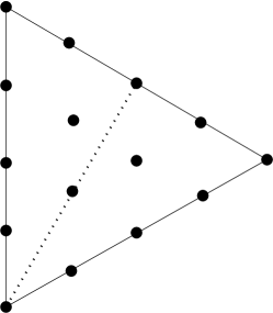
Figure 2: $SU(3)$: 15 vacuum states for $k=4$. The dotted line marks the boundary of the Weyl alcove for $G_{2}$.

For a generic $k$, the number of the states is

$$I^{\rm tree}_{SU(3)}(k>0)\ =\ \sum_{m=1}^{k+1}m\ =\ \frac{(k+1)(k+2)}{2}\ .$$ (2.19)

The analysis for $SU(4)$ is similar. The Weyl alcove is the tetrahedron with the vertices corresponding to cenral elements of $SU(4)$. A pure geometric computation gives

$$I^{\rm tree}_{SU(4)}(k>0)\ =\ \sum_{m=1}^{k+1}\sum_{p=1}^{m}p\ =\ \frac{(k+1)(k+2)(k+3)}{6}\ .$$ (2.20)

The generalization for an arbitrary $N$ is obvious. It gives the result

$$I^{\rm tree}(k,N)\ =\ \left(\begin{array}[]{c}k+N-1\\ N-1\end{array}\right)\$$ (2.23)

We also performed a similar analysis for the symplectic groups and for $G_{2}$. Let us dwell on $G_{2}$. The simple coroots for $G_{2}$ are ${\bf a}=(1,0)$ and ${\bf b}=(-3/2,\sqrt{3}/2)$. The lattice of coroots and the maximal torus look exactly in the same way as for $SU(3)$ (Fig. 3). Hence, before Weyl-invariance requirement is imposed, the index is equal to $3k^{2}$, as for $SU(3)$. The difference is that the Weyl group involves now 12 rather than 6 elements, and the Weyl alcove is half size of that for $SU(3)$. As a result, for $k=4$, we have only 9 (rather than 15) Weyl-invariant states (see Fig.2). The general formula is

$$I^{\rm tree}_{G_{2}}(k)\ =\ \left\{\begin{array}[]{c}\frac{(|k|+2)^{2}}{4}\ \ \ \ \ \ \ \ \ {\rm for\ even}\ k\\ \frac{(|k|+1)(|k|+3)}{4}\ \ \ \ \ \ \ \ {\rm for\ odd}\ k\end{array}\right\}\ .$$ (2.26)

Figure 3: Coroot lattice and Weyl alcove for $G_{2}$.

3 Loop corrections.

We will mostly discuss in this section the $SU(2)$ theory. For a generalization of all arguments to higher-rank groups, we refer the reader to [28].

3.1 Infinite volume.

It has been known since [29] that the CS coupling $\kappa$ in the pure YMCS theory is renormalized at the 1-loop level. For ${\cal N}=1,2,3$  SYMCS theories, the corresponding calculations have been performed in [30]. The effect can be best understood by considering the fermion loop contribution to the renormalization of the structure $\propto A\partial A$ in the Chern-Simons term ( Fig.4). Recalling that $\kappa$ and $k$ are assumed to be positive by default, we obtain

Figure 4: Renormalization of the structure $\propto\epsilon_{\mu\nu\rho}{\rm Tr}\{A_{\mu}\partial_{\nu}A_{\rho}\}$ by a fermion loop.

$$\Delta\kappa\ =\ -mc_{V}\int\frac{d^{3}p_{E}}{(2\pi)^{3}}\frac{1}{(p_{E}^{2}+m^{2})^{2}}\ =\ -\frac{c_{V}}{8\pi}\,.$$ (3.1)

There is also a contribution coming from the gluon loop. It is convenient [2] to choose the Hamilton gauge $A_{0}=0$, in which case the gluon propagator

$$D_{jk}^{ab}(\omega,\vec{p})\ =\frac{ig^{2}\delta^{ab}}{\omega^{2}-\vec{p}^{2}-m^{2}}\left[\delta_{jk}-\frac{p_{j}p_{k}}{\omega^{2}}-\frac{im}{\omega}\epsilon_{jk}\right]$$ (3.2)

involves only transverse degrees of freedom and there are no ghosts.

An accurate calculation gives

$$k_{\rm ren}\ =\ k+c_{V}-\frac{c_{V}}{2}\,,$$ (3.3)

where the first term comes from the gluon loop and the second term from the fermion loop.

A legitimate question is whether the second and higher loops also bring about a renormalization of the level $k$. The answer is negative. The proof is simple. We consider the case $k\gg c_{V}$. This is the perturbative regime where the loop corrections are ordered such that $\Delta k^{\rm(1\ loop)}\sim O(1),\ \ \Delta k^{\rm(2\ loops)}\sim O(1/k)$, etc. But corrections to $k$ of the order $\sim 1/k$ are not allowed. To ensure gauge invariance, $k_{\rm ren}$ must be an integer. Hence, all higher loop contributions in $k_{\rm ren}$ must vanish, and they do.

Note finally that the renormalization (3.3) refers to supersymmetric Yang-Mills-Chern-Simons theory — dynamical theory with nontrivial interactions. There is no such renormalization in the topological pure supersymmetric Chern-Simons theory where the fermions decouple. The number of states in this theory is the same as in the pure CS theory.

3.2 Finite volume.

As was mentioned above, the coefficient $\kappa$ (with the factor $L^{2}$) has the meaning of the magnetic field on the dual torus for the effective finite-volume BO Hamiltonian. The renormalization of $\kappa$ translates into a renormalization of this magnetic field. At the tree level, the magnetic field was constant. The renormalized field is not constant, however, but depends on the slow variables $C_{j}$. To find this dependence, we have to evaluate the effective Lagrangian in the slow Abelian background $C_{j}(t)$. The effective vector potential is extracted from the term $\sim{\cal A}_{j}(\vec{C})\dot{C}_{j}$ in this Lagrangian. This term can be evaluated in the background field approach. Up to certain fine technical points [1, 2] that we will not discuss here, the result can be obtained by taking the same Feynman graphs that determined renormalization of $\kappa$ in the infinite volume and replacing

$$p_{j}\to\frac{2\pi n_{j}}{L}-C_{j}\,,\ \ \ \ \ \ \ \ \ \ \int\frac{d^{2}p}{(2\pi)^{2}}\to\frac{1}{L^{2}}\sum_{n_{j}}$$ (3.4)

in the spatial integrals there. The shift $-\vec{C}$ in the momentum is due to replacing the usual derivative by the covariant one.

For the effective vector-potentials induced by the fermion and the gluon loop, we derive

$${\cal A}_{j}^{F}\ =\ \frac{\epsilon_{jk}}{2}\sum_{n_{j}}\frac{\left(C-\frac{2\pi n}{L}\right)_{k}}{\left(\vec{C}-\frac{2\pi\vec{n}}{L}\right)^{2}}\left[1-\frac{m}{\sqrt{\left(\vec{C}-\frac{2\pi\vec{n}}{L}\right)^{2}+m^{2}}}\right]\ \stackrel{{\scriptstyle m\to 0}}{{\longrightarrow}}$$

$$\frac{\epsilon_{jk}}{2}\sum_{n_{j}}\frac{\left(C-\frac{2\pi n}{L}\right)_{k}}{\left(\vec{C}-\frac{2\pi\vec{n}}{L}\right)^{2}}$$ (3.5)

and

$${\cal A}_{j}^{B}\ =\ -\frac{\epsilon_{jk}}{2}\sum_{n_{j}}\frac{\left(C-\frac{2\pi n}{L}\right)_{k}}{\left(\vec{C}-\frac{2\pi\vec{n}}{L}\right)^{2}}\left[2-\frac{3m}{\sqrt{\left(\vec{C}-\frac{2\pi\vec{n}}{L}\right)^{2}+m^{2}}}\right.$$

$$\left.+\frac{m^{3}}{\left[\left(\vec{C}-\frac{2\pi\vec{n}}{L}\right)^{2}+m^{2}\right]^{3/2}}\right]\ \stackrel{{\scriptstyle m\to 0}}{{\longrightarrow}}\ -\epsilon_{jk}\sum_{n_{j}}\frac{\left(C-\frac{2\pi n}{L}\right)_{k}}{\left(\vec{C}-\frac{2\pi\vec{n}}{L}\right)^{2}}$$ (3.6)

The corresponding induced magnetic fields are

$$\Delta{\cal B}^{F}(\vec{C}) = -\frac{m}{2}\sum_{n_{j}}\frac{1}{\left[\left(\vec{C}-\frac{2\pi\vec{n}}{L}\right)^{2}+m^{2}\right]^{3/2}}\ ,$$ (3.7)

and

$$\Delta{\cal B}^{B}(\vec{C}) = \frac{3m}{2}\sum_{n_{j}}\frac{\left(\vec{C}-\frac{2\pi\vec{n}}{L}\right)^{2}}{\left[\left(\vec{C}-\frac{2\pi\vec{n}}{L}\right)^{2}+m^{2}\right]^{5/2}}\,.$$ (3.8)

For most values of $C_{j}$, the corrections (3.7), (3.8) are of order $\sim mL^{3}=\kappa g^{2}L^{3}$, which is small compared to ${\cal B}^{\rm tree}\sim\kappa L^{2}$ if $g^{2}L\ll 1$, which we assume. There are, however, four special points (the “corners” of the torus)

$$C_{j}=0,\ C_{j}=(2\pi/L,0),\ C_{j}=(0,2\pi/L),\ C_{j}=(2\pi/L,2\pi/L)\,,$$ (3.9)

at the vicinity of which the loop-induced magnetic field is much larger than the tree-level magnetic field. This actually means that the “Abelian” BO approximation, with an assumption that the energy scale associated with the slow variables $\{C_{j},\lambda\}$ is small compared to the energy scale of the non-Abelian components and higher Fourier modes, breaks down in this region.

Disregarding this for a while, one can observe that the loop corrections bring about effective flux lines similar to Abrikosov vortices located at the corners. The width of these vortices is of the order of $m$. Gluon corrections generate the lines of unite flux $\Phi^{B}=\frac{1}{2\pi}\int\Delta{\cal B}^{B}(\vec{C})\,d^{2}C\,=1$, while the fermion loops generate the lines of flux $\Phi^{F}=-1/2$. In total, we have a line of the flux $\Phi_{\rm line}=1/2$ in each corner.

Adding the induced fluxes to the tree-level flux, one obtains the total flux

$$\Phi^{\rm tot}=2k+4\cdot 1-4\cdot\frac{1}{2}=2k+2$$ (3.10)

suggesting the presence of $2k+2$ vacuum states in the effective BO Hamiltonian (before the Weyl invariance requirement is imposed).

Not all these states are admissible, however. The wave functions of four such states turn out to be singular at the corners, and they should be dismissed.

Indeed, we find the effective wave functions of all $2k+2$ states in the Abelian valley far enough from the corners (3.9). The effective vector potential corresponding to one of the loop-induced flux lines can be chosen in the form

$${\cal A}_{j}\ =\ -\frac{\epsilon_{jk}C_{k}}{2\vec{C}^{2}}F(m^{2},\vec{C}^{2})\,.$$ (3.11)

where the core profile function deduced from (3.2) and (3.2),

$$F(m^{2},\vec{C}^{2})\ =\ 1-\frac{2m}{\sqrt{\vec{C}^{2}+m^{2}}}+\frac{m^{3}}{\left(\vec{C}^{2}+m^{2}\right)^{3/2}}$$ (3.12)

vanishes at $C_{j}=0$ and tends to 1 for large $C_{j}$.

We consider the effective supercharge $Q^{\rm eff}$ given by (2.1) at the vicinity of the origin, but outside the core of the vortex (3.11),

$$m\ll C_{j}\ll 4\pi/L\,.$$ (3.13)

We can then set $F(m^{2},\vec{C}^{2})=1$, neglect the contribution of other flux lines as well as the homogeneous field contribution (2.3). The equation $Q^{\rm eff}\chi^{\rm eff}=0$ for a vacuum effective wave function acquires the form

$$\left(\frac{\partial}{\partial z}+\frac{1}{4z}\right)\chi^{\rm eff}\ =\ 0$$ (3.14)

(we recall that $z=\frac{C_{+}L}{4\pi}$). Its solution is

$$\chi^{\rm eff}(z,\bar{z})\sim\frac{F(\bar{z})}{z^{1/4}}\,.$$ (3.15)

The effective wave function on the entire torus can be restored from two conditions:

• it must behave as in (3.15) at the vicinity of each corner;

• it must satisfy the boundary conditions with the twist (2.7) corresponding to the total flux (3.10).

This gives the structure

$$\chi^{\rm eff}_{m}(z,\bar{z})\ \propto\frac{Q^{2k+2}_{m}(\bar{z})}{[\Pi(z)\Pi(\bar{z})]^{1/4}}\,,$$ (3.16)

where

$$\Pi(\bar{z})=Q^{4}_{3}(\bar{z})-Q_{1}^{4}(\bar{z})\,.$$ (3.17)

is a $\theta$ function of level 4 having zeros at the corners (3.9).

We can return now to the sums in (3.2), (3.2). The divergences can be regularized by subtracting from ${\cal A}_{j}$ a certain infinite pure gauge part $\sim\partial_{j}f(\vec{C})$ [as a side remark, this regularization breaks the apparent periodicity of (3.2), (3.2)]. After that, the massless limits of ${\cal A}_{+}^{F,B}$ and ${\cal A}_{-}^{F,B}$ represent meromorphic toric functions $P(\bar{z}),P(z)$ having simple poles at the corners (3.9). They are obviously expressed via $\Pi^{-1}(\bar{z})$ and $\Pi^{-1}(z)$.

The full wave function is the product of the effective wave function (3.16) and the ground state wave function of the fast Hamiltonian. Near the corner ${\bf C}=0$ in the region (3.13), the latter behaves as $\Psi^{\rm fast}\ \sim 1/\sqrt{|z|}$ [see Eq.(3.16) in Ref. [2]], which is extended to the behavior

$$\Psi^{\rm fast}\ \sim\frac{1}{\sqrt{|\Pi(z)|}}\,.$$ (3.18)

in the whole Abelian valley. Therefore, generically, the full wave function thus obtained is singular at the corners,

$$\Psi^{\rm fast}\chi^{\rm eff}_{m}(z,\bar{z})\ \sim\ \frac{1}{|\Pi(z)|}\,.$$ (3.19)

The singularity in ${\cal A}_{j}$ smears out when taking into account the finite core size suggesting that the singularity in the effective wave function smears out too. However, we do not actually have a right to go inside the core in the Abelian BO framework: this approximation breaks down there, as we mentioned.

An accurate corner analysis (which is again a Born-Oppenheimer analysis, where we have to treat as slow all zero Fourier modes of the fields, both the Abelian and non-Abelian) that involves the matching of the corner wave function to the wave function in the Abelian valley far from the corners was performed in [2]. The result is rather natural. It turns out that the singularity is not smeared out when going into the vortex core. In other words, the states whose Abelian BO wave functions exhibit a singularity at the corners in the massless limit, as in (3.19), stay singular there in the exact analysis with finite mass. Such states are not admissible and should be disregarded.

The admissible wave functions still have the structure (3.16), but theta functions $Q^{2k+2}_{m}(\bar{z})$ should have zeros at the corners. In other words, they can be presented as $\Pi(\bar{z})$ times a theta function of level $2k-2$. This gives

$$\chi^{\rm eff}_{m}(z,\bar{z})\ \propto{Q^{2k-2}_{m}}(\bar{z})\,\Pi^{3/4}(\bar{z})\,\Pi^{-1/4}(z)\,,$$ (3.20)

The parameter $m$ takes now $2k-2$ values, which gives $2k-2$ [rather than $2k+2$ as would follow naively from (3.16)] “pre-Weyl” vacuum states. After imposing the Weyl-invariance condition, we obtain $k$ states in agreement with (1.9).

The following important remark is of order here. We have obtained $2k-2$ pre-Weyl states by selecting $2k-2$ nonsingular states out of $2k+2$ states in Eq. (3.16). This equation was obtained by taking both gluon-induced and fermion-induced flux lines into account. However, it is possible to eliminate the gluon flux lines altogether.

In the region outside the vortex core where the BO approximation works, one can translate the effective Lagrangian analysis leading to (3.7) and (3.8) to the effective Hamiltonian analysis. The induced vector-potentials are then obtained as Pancharatnam-Berry phases [32, 33],

$${\cal A}_{j}^{\rm PB}=-i\frac{\int(\Psi^{\rm fast})^{*}\frac{\partial}{\partial C_{j}}\Psi^{\rm fast}\,dx^{\rm fast}}{\int(\Psi^{\rm fast})^{*}\Psi^{\rm fast}\,dx^{\rm fast}}$$ (3.21)

The potentials leading to (3.7) and (3.8) correspond to a particular choice of $\Psi^{\rm fast}$.

But we can as well modify the definition of the fast wave function by mutiplying it by any function of slow variables. In particular, we can multiply it by a factor that is singular at the origin ( the BO approximation is not applicable there anyway) and define

$$\tilde{\Psi}^{\rm fast}\ =\ \Psi^{\rm fast}\sqrt{\frac{\Pi(\bar{z})}{\Pi(z)}}\,.$$ (3.22)

One cannot decide between $\Psi^{\rm fast}$ and $\tilde{\Psi}^{\rm fast}$ in the Abelian BO framework. Evaluating (3.21) with $\tilde{\Psi}^{\rm fast}$ brings about an extra gradient term [cf. (2.4)] giving a negative unit flux line in each corner. It annihilates the fluxes induced by gluon loops. Now, the equation $Q^{\rm eff}\tilde{\chi}^{\rm eff}=0$ reads

$$\left(\frac{\partial}{\partial z}-\frac{1}{4z}\right)\chi^{\rm eff}\ =\ 0$$ (3.23)

with the solution $\chi^{\rm eff}\sim z^{1/4}F(\bar{z})$. Its extension to the entire torus is

$$\tilde{\chi}^{\rm eff}_{m}(z,\bar{z})\ \propto{Q^{2k-2}_{m}}(\bar{z})\,\sqrt{|\Pi(z)|}\,,$$ (3.24)

When multiplying by $\tilde{\Psi}^{\rm fast}$, these functions (all of which should be taken into account now) give exactly the same full wave functions as before. One can thus say that gluon-induced flux lines (more generally, any flux line with integer flux) should be disregarded in counting vacua. Such flux lines (kinds of Dirac strings) are simply not observable. On the other hand, vortices with fractional fluxes affect vacuum counting. Heuristically, four half-integer flux lines in a sense “disturb” this counting making it “more difficult” for the toric vacuum wave functions to stay uniquely defined (a single half-integer flux line would make it just impossible) such that the number of states is decreased.

For all other groups, the gluon loops should also be disregarded (which was recently proved in [28]) and the index is obtained by substituting the value of $k$ renormalized by exclusively fermion loops, $k\to k-c_{V}/2$ in the tree-level result. We arrive at the result (1.8) for $SU(N)$. For $G_{2}$, we obtain

$$I^{\rm SYMCS}_{{\cal N}=1}[G_{2}]\ =\ \left\{\begin{array}[]{c}\frac{k^{2}}{4}\ \ \ \ \ \ \ \ \ {\rm for\ even\ }k\\ \frac{k^{2}-1}{4}\ \ \ \ \ \ \ \ \ {\rm for\ odd\ }k\end{array}\right.\ .$$ (3.27)

For completeness, we also give here the result for the index for the symplectic groups. For positive $k$,

$$I^{\rm SYMCS}_{{\cal N}=1}[Sp(2r)]\ =\ \left(\begin{array}[]{c}k+\frac{r-1}{2}\\ r\end{array}\right)\,.$$ (3.30)

For negative $k$, the index is restored via $I(k)=(-1)^{r}I(-k)$.

4 Theories with matter.

In theories with matter, the index is modified compared to the pure SYMCS theories due to two effects:

• an extra matter-induced renormalization of $k$;

• the appearance of extra Higgs vacua due to nontrivial Yukawa interactions.

The first effect seems to be rather transparent: extra fermion loops bring about extra renormalization. There are, however, subtleties to be discussed later. As regards the extra Higgs vacua, their appearance is not limited to three dimensions, they also appear (and modify the index) in $4d$ supersymmetric gauge theories. We discuss this first.

4.1 $4d$ theories.

Historically, it was argued in Ref. [18] that adding nonchiral matter to a theory does not change the estimate for the index. Indeed, nonchiral fermions (and their scalar superpartners) can be given a mass. For large masses, they seem to decouple and the index seems to be the same as in the pure SYM theory .

However, it was realized later that, in some cases, massive matter can affect the index. The latter may change when in addition to the mass term, Yukawa terms that couple different matter multiplets are added. The simplest example is the ${\cal N}=1$ $SU(2)$ theory involving a couple of fundamental matter multiplets $Q^{j}_{f}$ ($j=1,2$ being the color and $f=1,2$ the subflavor index; the indices are raised and lowered with $\epsilon^{jk}=-\epsilon_{jk}$ and $\epsilon^{fg}=-\epsilon_{fg}$) and an adjoint multiplet $\Phi_{j}^{k}=\Phi^{a}(t^{a})_{j}^{k}$.

Let the tree superpotential be

$${\cal W}^{\rm tree}=\mu\Phi^{j}_{k}\Phi^{k}_{j}+\frac{m}{2}Q^{j}_{f}Q^{f}_{j}+\frac{h}{\sqrt{2}}Q_{jf}\Phi^{j}_{k}Q^{kf}\,,$$ (4.1)

where $\mu$ and $m$ are adjoint and fundamental masses, and $h$ is the Yukawa constant.

There is also the instanton-generated superpotential [38],

$${\cal W}^{\rm inst}\ =\ \frac{\Lambda^{5}}{V}\,,$$ (4.2)

where $\Lambda$ is a constant with the dimension of mass and $V=Q^{j}_{f}Q^{f}_{j}/2$ is the gauge-invariant moduli. Eliminating $\Phi$, we obtain the effective superpotential

$${\cal W}^{\rm eff}\ =\ mV-\frac{h^{2}V^{2}}{4\mu}+\frac{\Lambda^{5}}{V}\,.$$ (4.3)

The vacua are given by the solutions to the equation $\partial{\cal W}^{\rm eff}/\partial V=0$. This equation is cubic, and hence there are three roots and three vacua.

We now note that, when $h$ is very small, one of these vacua is characterized by a very large value, $\langle V\rangle\approx 2\mu m/h^{2}$ (and the instanton term in the superpotential plays no role here). In the limit $h\to 0$, it runs to infinity and we are left with only two vacua, the same number as in the pure SYM $SU(2)$ theory. Another way to see it is to observe that the equation $\partial{\cal W}^{\rm eff}/\partial V=0$ becomes quadratic for $h=0$ having only two solutions.

The same phenomenon shows up in the theory with the $G_{2}$ gauge group studied in [40]. This theory involves three 7-plets $S^{j}_{f}$. The index of a pure SYM with $G_{2}$ group is known to coincide with the adjoint Casimir eigenvalue $c_{V}$ of $G_{2}$. It is equal to 4. However, if we include the Yukawa term,

$${\cal W}^{\rm Yukawa}\ =\ h\,\epsilon^{fgh}f^{jkl}S_{fj}S_{gk}S_{hl}$$ (4.4)

in the superpotential ($f^{jkl}$ being the Fano antisymmetric tensor), two new vacua appear. They tend to infinity in the limit $h\to 0$.

The appearance of new vacua when Yukawa terms are added should by no means come as a surprise. This basically occurs because the Yukawa term has a higher dimension than the mass term.

4.2 $3d$ superspace.

We use a variant of the ${\cal N}=1$ $3d$ superspace formalism developped in [41]. The superspace $(x^{\mu},\theta^{\alpha})$ involves a real 2-component spinor $\theta^{\alpha}$. Indices are lowered and raised with antisymmetric $\epsilon_{\alpha\beta},\epsilon^{\alpha\beta}$, $\theta^{2}\equiv\theta^{\alpha}\theta_{\alpha}$, $\int\,d^{2}\theta\,\theta^{2}=-2$. The $3d$ $\gamma$-matrices $(\gamma^{\mu})^{\alpha}_{\ \beta}$ chosen as in (1.3) satisfy the identity

$$\gamma^{\mu}\gamma^{\nu}\ =\ g^{\mu\nu}+i\epsilon^{\mu\nu\rho}\gamma_{\rho},\,.$$ (4.5)

Note that $(\gamma^{\mu})_{\alpha\beta}$ are all imaginary and symmetric.

Gauge theories are described in terms of the real spinorial superfield $\Gamma_{\alpha}$. For non-Abelian theories, the $\Gamma_{\alpha}$ are Hermitian matrices. As in $4d$, one can choose the Wess-Zumino gauge reducing the number of components of $\Gamma_{\alpha}$. In this gauge,

$$\Gamma_{\alpha}=i(\gamma^{\mu})_{\alpha\beta}\theta^{\beta}A_{\mu}+i\theta^{2}\lambda_{\alpha}\,,$$ (4.6)

The covariant superfield strength is then

$$W_{\alpha}\ =\ \frac{1}{2}{\cal D}^{\beta}{\cal D}_{\alpha}\Gamma_{\beta}-\frac{1}{2}[\Gamma^{\beta},{\cal D}_{\beta}\Gamma_{\alpha}]$$

$$=-i\lambda_{\alpha}+\frac{1}{2}\epsilon^{\mu\nu\rho}F_{\mu\nu}(\gamma_{\rho})_{\alpha\beta}\theta^{\beta}+\frac{i\theta^{2}}{2}(\gamma^{\mu})^{\beta}_{\ \alpha}\nabla_{\mu}\lambda_{\beta}\,,$$ (4.7)

In the superfield language, the Lagrangian (1.2) is written as

$${\cal L}\ =\ \int d^{2}\theta\left\langle\frac{1}{2g^{2}}W_{\alpha}W^{\alpha}+\ \frac{i\kappa}{2}\left(W_{\alpha}\Gamma^{\alpha}+\frac{1}{3}\{\Gamma^{\alpha},\Gamma^{\beta}\}{\cal D}_{\beta}\Gamma_{\alpha}\right)\right\rangle\,.$$ (4.8)

We now add matter multiplets. In this talk, we will consider only real adjoint multiplets. (In Ref.[3], we also treat the theories with complex fundamental multiplets.) Let there be only one such multiplet,

$$\Sigma=\sigma+i\psi_{\alpha}\theta^{\alpha}+i\theta^{2}D\,.$$ (4.9)

The gauge invariant kinetic term has the form

$${\cal L}^{\rm kin}=-\frac{1}{2g^{2}}\int d^{2}\theta\left\langle\nabla_{\alpha}\Sigma\,\nabla^{\alpha}\Sigma\right\rangle\,,$$ (4.10)

where $\nabla_{\alpha}\Sigma={\cal D}_{\alpha}\Sigma-[\Gamma_{\alpha},\Sigma]$. One can add also the mass term ,

$${\cal L}_{M}\ =\ -i\zeta\int d^{2}\theta\langle\Sigma^{2}\rangle\,.$$ (4.11)

Adding (4.8), (4.10), (4.11), expressing the Lagrangian in components, and eliminating the auxiliary field $D$, we obtain

$${\cal L}\ =\ \frac{1}{g^{2}}\left\langle-\frac{1}{2}F_{\mu\nu}^{2}+\nabla_{\mu}\sigma\nabla^{\mu}\sigma+\lambda/\!\!\!\!\nabla\lambda+\psi/\!\!\!\!\nabla\psi\right\rangle$$

$$+\kappa\left\langle\epsilon^{\mu\nu\rho}\left(A_{\mu}\partial_{\nu}A_{\rho}-\frac{2i}{3}A_{\mu}A_{\nu}A_{\rho}\right)+i\lambda^{2}\right\rangle+i\zeta\langle\psi^{2}\rangle-\zeta^{2}g^{2}\langle\sigma^{2}\rangle\,.$$ (4.12)

Besides the gauge field, the Lagrangian involves the adjoint fermion $\lambda$ with the mass $m_{\lambda}=\kappa g^{2}$, the adjoint fermion $\psi$ with the mass $m_{\psi}=\zeta g^{2}$ and the adjoint scalar $\sigma$ with the same mass. The point $\zeta=\kappa$ is special. In this case, the Lagrangian (4.2) enjoys ${\cal N}=2$ supersymmetry.

4.3 Index calculations

We consider the theory defined by (4.2). First, let $\zeta>0$. Then the mass of the matter fermions is positive. To be more precise, it has the same sign as the gluino mass for $k>0$. The matter loops lead to an extra renormalization of $k$.

We note that the status of this renormalization is different from the one due to the gluino loop. We have seen that for the latter, the induced magnetic field on the dual torus is concentrated at the corners (3.9), which follows from the equality $m_{\lambda}L\ll 1$. On the other hand, the mass of the matter fields $m_{\psi}=\zeta g^{2}$ is an independent parameter. It is convenient to make it large, $m_{\psi}L\gg 1$. For a finite mass, the induced magnetic field has the form as in Eq.(3.7). For small $m_{\psi}L$, it is concentrated at the corners. But in the opposite limit, the induced flux density becomes constant, as the tree flux density is.

Thus, massive enough matter brings about a true renormalization of $k$ without any qualifications (sine sale if you will).

For positive $\zeta$, the renormalization is negative, $k\to\ k-1$. The index coincides with the index of the ${\cal N}=1$ SYMCS theory with a renormalized $k$,

$$I_{\zeta>0}=k-1\,.$$ (4.13)

For $k=1$, the index is zero and supersymmetry is spontaneously broken.

For negative $\zeta$, two things happen.

• First, the fermion matter mass has the opposite sign and so does the renormalization of $k$ due to the matter loop. We seem to obtain $I_{\zeta<0}=k+1$.

• This is wrong, however, due to another effect. For a positive $\zeta$, the ground state wave function in the matter sector is bosonic. But for a negative $\zeta$, it is fermionic, $\Psi\propto\prod_{a}\psi^{a}$, changing the sign of the index.

We obtain

$$I_{\zeta<0}=-k-1\,.$$ (4.14)

Supersymmetry is broken here for $k=-1$.

As was mentioned, the Lagrangian (4.2) with $\zeta=\kappa$ enjoys the extended ${\cal N}=2$ supersymmetry. That means, in particular, that $\zeta$ changes a sign together with $\kappa$ and the result is given by

$$I^{\rm SYMCS}_{{\cal N}=2}\ =\ |k|-1$$ (4.15)

in agreement with [45, 46]. In contrast to (4.13) and (4.14), this expression is not analytic at $k=0$, the nonanalyticity being due just to the sign flip of the matter fermion mass.

Strictly speaking, formula (4.15) does not work for $k=0$. In this case, we should also keep $\zeta=0$, the matter is massless, massless scalars make the motion infinite, and the index is ill-defined. However, bearing in mind that the regularized theory with $\zeta\neq 0$ gives the result $I^{\rm SYMCS}_{{\cal N}=2\ {\rm deformed}}(0)=-1$, irrespectively of the sign of $\zeta$, one can attribute this value for the index also to $I^{\rm SYMCS}_{{\cal N}=2}(0)$.

The three index formulas (4.13), (4.14), and (4.15) are represented together in Fig. 5.

Figure 5: The indices in the theory (4.2) with $\zeta>0$, $\zeta<0$, and $\zeta=\kappa$ (bold lines).

We next consider the theory involving a gauge multiplet (4.6) and three ${\cal N}=1$ real adjoint matter multiplets (4.9). If all the masses are equal, the theory has the extended ${\cal N}=2$ supersymmetry provided an extra Yukawa term is added in the Lagrangian [47]. If we call one of the matter multiplets (the one that forms together with (4.6) a ${\cal N}=2$ superfield) $\Sigma$ and combine two other real multiplets into the complex ${\cal N}=2$ multiplet $\Phi$, then the Yukawa term acquires the form

$${\cal L}_{\rm Yukawa}\ =-\frac{2i}{g^{2}}\int d^{2}\theta\,\langle\Sigma\Phi\bar{\Phi}\rangle\,.$$ (4.16)

To calculate the index, however, we will consider the deformed ${\cal N}=1$ Lagrangian with different masses $M$ (the mass of the field $\Sigma$) and $m$ (the mass of the complex field $\Phi$). We assume $M$ to be large, but, to make the transition to the ${\cal N}=2$ theory smooth, its sign to coincide with the sign of $k$.

There are four different cases:

1. $m>0,\ \ k>0\Rightarrow M>0$.

   $$k\to k-1_{\Sigma}-2_{\Phi}=k-3\,.$$ (4.17)

   This contributes $k-3$ to the index. Note that, for $k=1,2$, this contribution is negative.

2. $m>0,\ \ k,M<0$.

   $$k\to k+1_{\Sigma}-2_{\Phi}=k-1$$ (4.18)

   Multiplying it by -1 due to the fermionic nature of the wave function [ in this case, it involves a fermionic factor associated with the real adjoint matter multiplet $\Sigma$; see the discussion before Eq.(4.14)], we obtain $I=-k+1$.

3. $m<0,\ \ k,M>0$.

   $$k\to k-1_{\Sigma}+2_{\Phi}=k+1\,,$$ (4.19)

   giving the contribution $I=k+1$.

4. $m<0,\ \ k,M<0$.

   $$k\to k+1_{\Sigma}+2_{\Phi}=k+3\,.$$ (4.20)

   The contribution to the index is $-k-3$.

In contrast to the model with only one real adjoint multiplet, this is not the full answer yet. There are also additional states on the Higgs branch that contribute to the index. Indeed, the superpotential is

$${\cal W}\ =\ \frac{-i}{g^{2}}\left(\frac{M}{2}\Sigma^{a}\Sigma^{a}+m\bar{\Phi}^{a}\Phi^{a}+i\epsilon^{abc}\Sigma^{a}\Phi^{b}\bar{\Phi}^{c}\right)\,.$$ (4.21)

The bosonic potential vanishes provided

$$m\phi^{b}\ =\ i\epsilon^{abc}\sigma^{a}\phi^{c}\,,$$

$$M\sigma^{a}\ =\ i\epsilon^{abc}\bar{\phi}^{b}\phi^{c}\,.$$ (4.22)

These equations have nontrivial solutions when both $M$ and $m$ are positive or when both $M$ and $m$ are negative. Let them be positive. Then (4.3) has a unique solution up to a gauge rotation.

$$\sigma^{a}\ =\ m\left(\begin{array}[]{c}0\\ 0\\ 1\end{array}\right),\ \ \ \ \ \ \phi^{a}=\sqrt{\frac{Mm}{2}}\left(\begin{array}[]{c}1\\ -i\\ 0\end{array}\right)\,.$$ (4.29)

The corresponding contribution to the index is not just equal to 1, however, due to a new important effect that did not take place in $4d$ theory with superpotential (4.1) considered above and would also be absent in a $3d$ theory with a fundamental ${\cal N}=2$ matter multiplet.

Indeed, besides the solution (4.29), there are also the solutions obtained from that by gauge transformations. The latter are not necessarily global, they might depend on the spatial coordinates $x,y$. We note that, for the theory defined on a torus, certain transformations can be applied to (4.29) that look like gauge transformations, but are not contractible due to the nontrivial $\pi_{1}[SO(3)]=Z_{2}$. (Here, $SO(3)$ should be understood not as the orthogonal group itself, but rather as the adjoint representation space; cf. the discussion of higher isospins below.) An example of such a quasi-gauge transformation is

$$\Omega_{1}:O^{ab}(x)\ =\ \left(\begin{array}[]{ccc}\cos\left(\frac{2\pi x}{L}\right)&\sin\left(\frac{2\pi x}{L}\right)&0\\ -\sin\left(\frac{2\pi x}{L}\right)&\cos\left(\frac{2\pi x}{L}\right)&0\\ 0&0&1\end{array}\right)\,,$$ (4.33)

where $L$ is the length of our box. The transformation (4.33) does not affect $\sigma^{a}=\sigma\delta^{a3}$ and keeps the fields $\phi^{a}(\vec{x})$ periodic. There is a similar transformation $\Omega_{2}$ along the second cycle of the torus.

In $4d$ theories, wave functions are invariant under contractible gauge transformations. In $3d$ SYMCS theories, they are invariant up to a possible phase factor, as in (2.1). But nothing dictates the behaviour of the wave functions under the transformations $\Omega_{1,2}$ which are actually not gauge symmetries, but rather some global symmetries of the theory living on a torus. We thus obtain four different wave functions, even or odd under the action of $\Omega_{1,2}$. The final result for the index of this theory is

$$I^{{\cal N}=2}_{\rm adjoint\ matter}\ =\ |k|+1\,.$$ (4.34)

universally for positive and negative $k$. Extra Higgs states contribute only for positive $k$.

The result (4.34) was derived among others in [24] following a different logic. Intriligator and Seiberg did not deform ${\cal N}=2\ \to{\cal N}=1$, but kept the fields in the real adjoint matter multiplet $\Sigma$ light. Then the light matter fields $\{\sigma,\psi\}$ enter the effective BO Hamiltonian at the same ground as the Abelian components of the gluon and gluino fields. As was mentioned, the fluxes induced by the light fields are not homogeneous being concentrated at the corners. This makes an accurate analysis substantially more difficult. The index (4.34) was obtained in [24] as a sum of three rather than just two contributions and it is still not quite clear how this works in the particular case $k=2$ where $k_{\rm eff}$ as defined in Ref.[24] and including only renormalizations due to complex matter multiplet, $k_{\rm eff}=k-2$, vanishes.

Our method is simpler.

We can also add the ${\cal N}=2$ multiplets with higher isospins. Then the counting of Higgs vacuum states becomes more complicated. For example, for $I=3/2$, there are 10 such states. This number is obtained as a sum of the single state with the isospin projection $1/2$ and $3^{2}=9$ states with the isospin projection $3/2$ (in the latter case, there is a constant solution supplemented by eight $\vec{x}$-dependent quasi-gauge copies). The generic result for the index in the theory involving several ${\cal N}=2$ matter multiplets with different isospins is

$$I=|k|-1+\frac{1}{2}\sum_{f}T_{2}(I_{f})\,,$$ (4.35)

where

$$T_{2}(I)\ =\frac{2I(I+1)(2I+1)}{3}$$ (4.36)

is the Dynkin index of the corresponding representation normalized to $T_{2}({\rm fund})=1$.

When deriving (4.35), it was assumed that the matter-induced shift of the index is the sum of the individual shifts due to individual multiplets. This is true if the Lagrangian does not involve extra cubic ${\cal N}=2$ invariant superpotentials which can bring about extra Higgs vacuum states.

We can observe that the index does not depend on the sign of $k$, although this universal result is obtained by adding the contributions that look completely different for $k>0$ and $k<0$. For an individual multiplet contribution, the Higgs states contribute only for one sign of $k$ (positive or negative depending on the sign of the mass). An interesting explanation of the symmetry under the mass sign flip with a given $k$ (and hence under the sign flip of $k$ with a given $m$) was suggested in [24]. Basically, the authors argued that one can add to the mass the size of one of the dual torus cycles times $i$ to obtain a complex holomorphic parameter on which the index of an ${\cal N}=2$ theory should not depend. Hence, it should not depend on the real part of this parameter (the mass). We believe that it is still dangerous to pass the point $m=0$ where the index is not defined and this argument therefore lacks rigour. Anyway, an explicit $SU(2)$ calculation shows that the symmetry with respect to mass sign flip is indeed maintained.

The reasoning above can be generalized to higher-rank unitary groups. Intriligator and Seiberg conjectured the following generalization of (4.35),

$$I^{SU(N)} = \frac{1}{(N-1)!}\prod_{j=-\frac{N}{2}+1}^{\frac{N}{2}-1}\left(|k|+\frac{1}{2}\sum_{f}T_{2}(R_{f})-\frac{N}{2}-j\right)\,,$$ (4.37)

implying that the overall shift of $k$ is represented as the sum of individual shifts due to indivudual multiplets. For an individual contribution to the shift, this formula can be derived for different signs of $k$ and $m$ when the extra Higgs states do not contribute. It can be extended to $k,m$ of the same sign using the symmetry discussed above.

We checked that this works for all $SU(N)$ groups with fundamental matter and for $SU(3)$ with adjoint matter. It would be interesting to construct a rigourous proof of this fact.

Appendix A. Theta functions.

We here recall certain mathematical facts concerning the properties of analytical functions on a torus. They are mostly taken from the textbook [49], but we are using a different notation, which we find clearer and more appropriate for our purposes.

Theta functions play the same role for the torus as ordinary polynomials for the Riemann sphere. They are analytic, but satisfy certain nontrivial quasiperiodic boundary conditions with respect to shifts along the cycles of the torus. A generic torus is characterized by a complex modular parameter $\tau$, but we will stick to the simplest choice $\tau=i$ so that the torus represents a square $x,y\in[0,1]$ ( $z=x+iy$) glued around.

The simplest $\theta$-function satisfies the boundary conditions

$$\theta(z+1) = \theta(z)\,,$$

$$\theta(z+i) = e^{\pi(1-2iz)}\theta(z)\,.$$ (A.1)

This defines a unique (up to a constant complex factor) analytic function. Its explicit form is

$$\theta(z)\ =\ \sum_{n=-\infty}^{\infty}\,\exp\{-\pi n^{2}+2\pi inz\}\,.$$ (A.2)

This function (call it theta function of level 1 and introduce an alternative notation $\theta(z)\equiv Q^{1}(z)$) has only one zero in the square $x,y\in[0,1]$, exactly in its middle, $\theta(\frac{1+i}{2})=0$.

For any integer $q>0$, theta functions of level $q$ can be defined such that

$$Q^{q}(z+1) = Q^{q}(z)\,,$$

$$Q^{q}(z+i) = e^{q\pi(1-2iz)}Q^{q}(z)\,.$$ (A.3)

The boundary conditions (Appendix A. Theta functions.) involve the twist [the exponent in the R.H.S. of Eq. (2.7)] $-2\pi q$ corresponding to the negative magnetic flux. The functions $Q^{q}(\bar{z})$ have positive fluxes $2\pi q$. Multiplying $Q^{2k}(\bar{z})$ and $Q^{2k}(z)$ by proper exponentials, yields the functions (2.8) (no longer analytic) satisfying the boundary conditions (2.1).

The functions satisfying (Appendix A. Theta functions.) lie in a vector space of dimension $q$. The basis in this vector space can be chosen as

$$Q^{q}_{m}(z)\ =\ \sum_{n=-\infty}^{\infty}\,\exp\left\{-\pi q\left(n+\frac{m}{q}\right)^{2}+2\pi iqz\left(n+\frac{m}{q}\right)\right\}\,,$$

$$m=0,\ldots,q-1\,.$$ (A.4)

In Mumford’s notation [49], $Q^{q}_{m}(z)$ can be expressed as

$$Q^{q}_{m}(z)\ =\ \theta_{m/q,0}(qz,iq)\ ,$$ (A.5)

where $\theta_{a,b}(z,\tau)$ are theta functions of rational characteristics.

$Q^{q}_{m}(z)$ can be called “elliptic polynomials” of degree $q$. Indeed, each $Q^{q}_{m}(z)$ has $q$ simple zeros at

$$z_{s}^{(m)}\ =\ \frac{2s+1}{2q}+i\left(\frac{1}{2}-\frac{m}{q}\right)\,,\ \ \ \ \ \ \ s=0,\ldots,q-1$$ (A.6)

(add $i$ to bring it onto the fundamental domain $x,y\in[0,1]$ when necessary). A product $Q^{q}(z)Q^{q^{\prime}}(z)$ of two such “polynomials” of degrees $q,q^{\prime}$ gives a polynomial of degree $q+q^{\prime}$. There are many relations between the theta functions of different level and their products, which follow. We can amuse the reader with a relation

$$\frac{Q^{6}_{5}(z)-Q^{6}_{1}(z)}{(Q^{4}_{3}(z)-Q^{4}_{1}(z))Q^{2}_{0}(z)}\ =\ \frac{1}{\eta(i)}=\frac{2\pi^{3/4}}{\Gamma(1/4)}\,.$$ (A.7)

The ratios of different elliptic functions of the same level give double periodic meromorphic elliptic functions. For example, the ratio of a properly chosen linear combination $\alpha Q^{2}_{1}(z)+\beta Q^{2}_{2}(z)$ and $[\theta(z)]^{2}$ is the Weierstrass function.

References

- [1] A.V. Smilga, JHEP 1001 086 (2010) [ arXiv:0910.0803, hep-th].
- [2] A.V. Smilga, JHEP 1205 103 (2012) [arXiv:1202.6566, hep-th].
- [3] A.V. Smilga, arXiv:1308.5951, hep-th.
- [4] J. Bagger and N. Lambert, Phys. Rev. D 77:065008 (2008) [arXiv: 0711.0955, hep-th].
- [5] O. Aharony, O. Bergman, D.L. Jafferis and J. Maldacena, JHEP 0810:091 (2008), [arXiv:0806.1218, hep-th].
- [6] J.M. Maldacena, Adv. Theor. Math. Phys. 2 231 (1998).
- [7] S.S. Gubser, I.R. Klebanov, and A.M. Polyakov, Phys. Lett. B428 105 (1998).
- [8] A. Gorsky, Phys.Usp. 48 (2005) 1093-1108.
- [9] G. Romelsberger, Nucl. Phys. B 747 329 (2006) [hep-th/0510060].
- [10] V.P. Spiridonov and G.S. Vartanov, Nucl. Phys. B 824 192 (2010) [arXiv:0811.1909, hep-th].
- [11] G.V. Dunne, hep-th/9902115.
- [12] E. Witten, in: [Shifman, M.A. (ed.) The many faces of the superworld p.156] [ hep-th/9903005].
- [13] A.J. Niemi and G.W. Semenoff, Phys. Rev. Lett. 51 (1983) 2077.
- [14] N. Redlich, Phys. Rev. D29 (1984) 2366.
- [15] E. Witten, Commun. Math. Phys. 121 351 (1989).
- [16] S. Elitzur, G. Moore, A. Schwimmer, and N. Seiberg, Nucl. Phys. B 326 108 (1989).
- [17] J.M.F. Labastida and A.V. Ramallo, Phys. Lett. B 227 92 (1989).
- [18] E. Witten, Nucl. Phys. B 202 253 (1982).
- [19] M. Henningson, JHEP 1211 013 (2012) [arXiv: 1209.1798, hep-th].
- [20] V.G. Kac and A.V. Smilga, in: [Shifman, M.A. (ed.) The many faces of the superworld p.185] [ hep-th/9902029].
- [21] A. Keurentjes, JHEP 9905 (1999) 001 [hep-th/9901154].
- [22] A. Keurentjes, JHEP 9905 (1999) 014 [hep-th/9902186].
- [23] S. Deser, R. Jackiw, and S. Templeton, Ann. Phys. (NY) 140 372 (1982).
- [24] K. Intriligator and N. Seiberg, arXiv:1305.1633 [hep-th].
- [25] B.A. Dubrovin, I.M. Kričever, and S.P. Novikov, Soviet Math Dokl. 229 15 (1976).
- [26] B.A. Dubrovin and S.P. Novikov, Soviet Phys. JETP 79 1006 (1980).
- [27] S. Cecotti and L. Girardello, Phys.Lett. B 110 39 (1982).
- [28] A.V. Smilga, arXiv: 1404.2779.
- [29] R.D. Pisarski and S. Rao, Phys. Rev. D 32 2081 (1985).
- [30] H.-S. Kao, K. Lee, and T. Lee, Phys.Lett. B 373 94 (1996) [hep-th/9506170].
- [31] K. Gawedzki and A. Kupiainen, Nucl. Phys. B 320 625 (1989).
- [32] S. Pancharatnam, Proc. Indian Acad. Sci. A44 (1956) 247.
- [33] M. Berry, Proc. R. Soc. Lond. A392 (1984) 45.
- [34] A.V. Smilga, Soviet Phys. JETP 64 8 (1986).
- [35] B.Yu. Blok and A.V. Smilga, Nucl. Phys. B 287 589 (1987).
- [36] K. Intriligator and N. Seiberg, Nucl. Phys. B 431 551 (1994) [hep-th/9408155].
- [37] A. Gorsky, A. Vainshtein, and A. Yung, Nucl. Phys. B 584 197 (2000) [hep-th/0004087].
- [38] I. Affleck, M. Dine, and N. Seiberg, Phys. Lett. B 137 187 (1984).
- [39] N. Seiberg and E. Witten, Nucl. Phys. B 431 484 (1994) [hep-th/9408099].
- [40] A. Smilga, Phys. Rev. D 58 105014 (1998) [hep-th/9801078].
- [41] S.J. Gates, M.T. Grisaru, M. Rocek, and W. Siegel, Front. Phys. 58 1-548 (1983) [hep-th/0108200].
- [42] H. Nishino and S.J. Gates, Int. J. Mod. Phys. A 8 3371 (1993).
- [43] O. Aharony et al., Nucl. Phys. B 499 67 (1997) [hep-th/9703110].
- [44] J. de Boer, K. Hori, and Y. Oz, Nucl. Phys. B 500 (1997) [hep-th/9703100].
- [45] K. Ohta, JHEP 9910 006 (1999) [hep-th/9908120].
- [46] O. Bergman, A. Hanany, A. Karch, and B. Kol JHEP 9910 036 (1999) [hep-th/9908075].
- [47] E.A. Ivanov, Phys. Lett. B 268 203 (1991).
- [48] G. ’t Hooft, Nucl. Phys. B 153 141 (1979).
- [49] D. Mumford, Tata Lectures on Theta (Birkhäuser Boston, 1983).