Sparse latent factor models with interactions: Analysis of gene expression data

Abstract

Sparse latent multi-factor models have been used in many exploratory and predictive problems with high-dimensional multivariate observations. Because of concerns with identifiability, the latent factors are almost always assumed to be linearly related to measured feature variables. Here we explore the analysis of multi-factor models with different structures of interactions between latent factors, including multiplicative effects as well as a more general framework for nonlinear interactions introduced via the Gaussian Process. We utilize sparsity priors to test whether the factors and interaction terms have significant effect. The performance of the models is evaluated through simulated and real data applications in genomics. Variation in the number of copies of regions of the genome is a well-known and important feature of most cancers. We examine interactions between factors directly associated with different chromosomal regions detected with copy number alteration in breast cancer data. In this context, significant interaction effects for specific genes suggest synergies between duplications and deletions in different regions of the chromosome.

T0Supported by Award Number U54CA112952 from the National Cancer Institute, by funding from the Measurement to Understand Re-Classification of Disease of Cabarrus and Kannapolis (MURDOCK) Study and by a grant from the NIH CTSA (Clinical and Translational Science Award) 1UL1RR024128-01 to Duke University.

and

t1This study was developed in the Ph.D. program of the Department of Statistical Science at Duke University where the first author received his Ph.D. degree.

1 Introduction

In recent years, numerous studies have applied factor models combined with the Bayesian framework to analyze gene expression data, and their results often show an improvement in the identification and estimation of metagene groups and patterns related to the underlying biology; see, for example, West (2003), Lucas et al. (2006) and Carvalho et al. (2008). The usual formulation for factor models assumes additive effects of latent factors across the samples. This assumption leads to very tractable model fitting and computation, but may not represent the reality in some applications. The structure of dependence between genes in biological pathways motivates the idea of a model with nonlinear interactions between latent factors. The presence of interactions can have important implications for the interpretation of the underlying biology.

The study of nonlinear interactions between observed variables has been the focus of many publications in the context of regression problems. In many cases, the proposed model introduces the nonlinearity through the specification of Gaussian Process (GP) priors. Henao and Winther (2010) consider sparse and identifiable linear latent variable (factor) and linear Bayesian network models for parsimonious analysis of multivariate data. The framework consists of a fully Bayesian hierarchy for sparse models using spike and slab priors, non-Gaussian latent factors and a stochastic search over the ordering of the variables. The authors argue that the model is flexible in the sense that it can be extended by only changing the prior distribution of a set of latent variables to allow for nonlinearities between observed variables through GP priors.

The nonlinear relationship between a set of observed variables is also the topic of Hoyer et al. (2009) in the context of Directed Acyclic Graphs (DAG). Each observed variable (node in a DAG) is obtained as a function of its parents plus independent additive noise. An arbitrary function is chosen to define linear/nonlinear relationships between the observed values. The paper evaluates whether a DAG is consistent with the data by constructing a nonlinear regression of each variable on its parents, and subsequently testing whether the resulting residuals are mutually independent. GP regression and kernelized independence tests are used in the paper.

Associations between observed and latent variables is another interesting topic. Arminger and Muthen (1998) consider latent variable models including polynomial terms and interactions of latent regressor variables. Two groups of observed variables are used: the response vector y, and the vector of covariates x. Their model specifies two equations; the first one expresses y as a linear combination of polynomial terms and/or interactions of elements in the latent vector $\xi$. The second equation defines a factor model without interaction terms, where $\xi$ is the factor score and x is the target data. Because the model includes components representing functions of latent variables in the first equation, the authors denote the formulation as nonlinear. They use the Bayesian framework with conjugate priors to estimate the parameters; sparsity priors are not considered in their analysis. In the spirit of factor analysis, Teh, Seeger and Jordan (2005) model the relationships among components of a response vector y using linear (or generalized linear) mixing of underlying latent variables indexed by a covariate vector x (observed values). The authors assume that each latent variable is conditionally independently distributed according to a GP, with x being the (common) index set. The mean of the response y is then a function of a linear combination of the conditionally independent GP.

Most applications of GP models involve learning tasks where both output and input data are assumed to be given at training time. Lawrence (2004) and Lawrence (2005) have proposed a multiple-output GP regression model assuming observed output data and latent variables as inputs. The approach explores nonlinear interactions between the latent factors. The authors introduce a probabilistic interpretation of principal component analysis (PCA) named dual probabilistic PCA (DPPCA). The DPPCA model has the advantage that the linear mappings from the latent-space to the data-space can be easily nonlinearized through Gaussian processes (DPPCA with a GP introducing nonlinearity is then called GP Latent Variable Model or GP-LVM). The GP (assumed for latent variables) with an inner product kernel in the covariance function defines a linear association, and it has an interpretation as a probabilistic PCA model. GP-LVM can be obtained by replacing this inner product kernel with a nonlinear covariance function. The nonlinear mappings are designed to address the weaknesses in visualizing data sets that arise when using statistical tools that rely on linear mappings, such as PCA and standard factor models. The analyses are based on optimization via maximum likelihood estimation; no MCMC algorithm is applied and no sparsity prior is assumed.

In GP models, inference is analytically tractable for regression problems, and deterministic approximate inference algorithms are widely used for classification problems. The use of MCMC methods to sample from posterior distributions in a model assuming GP prior has been explored in the literature only for cases with observed input data. As an example, Titsias, Lawrence and Rattray (2009) describe an MCMC algorithm which constructs proposal distributions by utilizing the GP prior. At each iteration, the algorithm generates control variables and samples the target function from the conditional GP prior. The control variables are auxiliary points associated with observed input variables defined in the model. An advantage of MCMC over deterministic approximate inference is that the sampling scheme will often not depend on details of the likelihood function, and is therefore very generally applicable. In addition, the development of deterministic approximations is difficult since the likelihood can be highly complex. Chen et al. (2010) have considered inference based on Variational Bayesian (VB) approximation and Gibbs sampling to examined distinct ways of inferring the number of factors in factor models applied to gene expression data. The study indicates that while the cost of each VB iteration is larger than that of MCMC, the total number of VB iterations is much smaller. However, the CPU cost of MCMC appears to be worthwhile, as they found that for a large-scale data set the MCMC results were significantly more reliable than VB; the VB approximation has difficulties with local-optimal solutions, and the factorized form of the VB posterior may not be as accurate for large-scale problems.

Different latent class models have been proposed in the literature to analyze the DNA Copy Number Alteration (CNA) problem. For example, Lucas, Kung and Chi (2010) use sparse latent factor analysis to identify CNA associated with the hypoxia and lactic acidosis response in human cancers. Specifically, they fit a latent factor model of the gene signatures in one data set of 251 breast tumors [Miller et al. (2005)] to generate 56 latent factors. These factors then allow for connections to be made between a number of different data sets, which can be used to generate biological hypotheses regarding the basis for the variation in the gene signatures. They have identified variation in the expression of several factors which are highly associated with CNAs in similar or distinct chromosomal regions. DeSantis et al. (2009) developed a supervised Bayesian latent class approach to evaluate CNA on array CGH data. The authors assume that tumors arise from subpopulations (latent classes) sharing similar patterns of alteration across the genome. The methodology relies on a Hidden Markov Model (HMM) to account for the dependence structure involving neighboring clones within each latent class. In particular, the approach provides posterior distributions that are used to make inferences about gains and losses in copy number. Fridlyand et al. (2004) proposed a discrete-state homogeneous HMM where underlying states are considered segments of a common mean. One of the goals of the procedure is to identify copy number transitions. Marioni et al. (2006) extended this approach by developing the method BioHMM for segmenting array CGH data into states with the same underlying copy number. They use a heterogeneous HMM with probability of transitioning between states depending on the distance between adjacent clones.

We are interested in the study of multi-factor models developed for the analysis of matrices representing gene expression patterns. Our goal is to investigate the existence of interaction effects involving latent factors. In order to test the significance of the interaction terms, the mixture prior with a point mass at zero and a Gaussian component (sometimes referred to as the “spike and slab” prior) is assumed. This type of prior has been used effectively to define the sparse structure in West (2003), Lucas et al. (2006), Carvalho et al. (2008) and others. The outline of this paper is as follows. In Section 2 we propose a factor model with multiplicative interactions between latent factors. Our approach for this problem has not yet been considered in the literature. Two strategies are used to introduce the interactions. Section 3 explores nonlinear structure of interactions between factors; the formulation is more general. In short, we introduce nonlinearities through the specification of a GP prior for a set of latent variables. Five different versions of the model are investigated; they differ in terms of prior formulations for probability parameters and the assumption regarding the similarity of the interaction effects for distinct features. In Section 4 a simulated study is developed to evaluate and compare the models from Sections 2 and 3. Additional synthetic data analyses to assess the performance of the models are presented in Mayrink and Lucas (2013). Sections 5 and 6 show real data applications where we examine interaction effects related to chromosomal regions detected with CNA in breast cancer data. Finally, Section 7 indicates the main conclusions and future work.

The algorithms required to fit the proposed models are implemented using the MATLAB programming language (http://www.mathworks.com).

2 Factor model with multiplicative interactions

Assume $X$ is an ($m\times n$) matrix with $X_{ij}$ representing gene $i$ and sample $j$. We propose the model

$$X=\alpha\lambda+\theta\eta+\varepsilon,$$ (1)

where $\alpha$ is an ($m\times L$) matrix of loadings, $\lambda$ is an ($L\times n$) matrix of factor scores, $\theta$ is an ($m\times T$) matrix of loadings, $\eta$ is a ($T\times n$) matrix of interaction effects, and $\varepsilon$ is an ($m\times n$) noise matrix with $\varepsilon_{ij}\sim N(0,\sigma_{i}^{2})$; let $\sigma^{2}=(\sigma_{1}^{2},\ldots,\sigma_{m}^{2})^{\prime}$. With this formulation, we are separating the linear and nonlinear effects. One could add the term $\mu 1_{n}$ in this model to estimate the mean expression of the genes; $\mu$ is an $m$-dimensional column vector and $1_{n}$ is an $n$-dimensional row vector of ones. We prefer the parsimonious version where the rows of $X$ are standardized and $\mu=\mathbf{0}$ is assumed.

The multiplicative interactions are defined in $\eta$ with the following assumption: $\eta_{1j}=\lambda_{1j}\lambda_{2j}$, $\eta_{2j}=\lambda_{1j}\lambda_{3j},\ldots,\eta_{Tj}=\lambda_{(L-1)j}\lambda_{Lj}$. Note that $T=L!/[(L-2)!2!]$.

In terms of prior distributions, we consider the conjugate specifications $\lambda_{lj}\sim N(0,1)$ and $\sigma_{i}^{2}\sim\mathit{IG}(a,b)$. In our study, the bimodal sparsity promoting priors are key elements in the structure of the model. This form of prior originated in the context of Bayesian variable selection, and it has been the subject of substantial research; see George and McCulloch (1993, 1997) and Geweke (1996). The spike and slab mixture prior is defined for the factor loadings to allow for sparsity and to test whether the factors/interactions have significant effect on each gene. Assume

$$\alpha_{il} \sim (1-h_{il})\delta_{0}(\alpha_{il})+h_{il}N(0,\omega_{\alpha}),$$

$$h_{il} \sim \operatorname{Bernoulli}(q_{il})\quad\mbox{and}\quad q_{il}\sim\operatorname{Beta}(\gamma_{1},\gamma_{2}),$$

$$\theta_{it} \sim (1-z_{it})\delta_{0}(\theta_{it})+z_{it}N(0,\omega_{\theta}),$$

$$z_{it} \sim \operatorname{Bernoulli}(\rho_{it})\quad\mbox{and}\quad\rho_{it}\sim\operatorname{Beta}(\beta_{1},\beta_{2}).$$

We consider two approaches to introduce the corresponding multiplicative interaction term; they are enumerated below: [(2)]

Introduce the interaction via Gaussian prior: $\eta_{tj}\sim N(\lambda_{l_{1}j}\lambda_{l_{2}j},\nu)$.

Assume the product with probability 1: $\eta_{tj}=\lambda_{l_{1}j}\lambda_{l_{2}j}$. In the cases above, let $l_{1}<l_{2}\in\{1,\ldots,L\}$ be the indices of factors involved in the product term related to $\eta_{tj}$ where $t\in\{1,\ldots,T\}$.

In the first version, we specify the product $\lambda_{l_{1}j}\lambda_{l_{2}j}$ as the mean parameter of the Gaussian distribution. This approach can be generalized with the specification of any function $f(\lambda_{l_{1}j},\lambda_{l_{2}j})$, which makes it possible to investigate other types of relationships between factors. The variance $\nu$ must have a small value; otherwise, we are indicating a weak association between $\eta_{tj}$ and $\lambda_{l_{1}j}\lambda_{l_{2}j}$. In this case, the multiplicative effect is lost and the interaction factor is just another factor in the model. If the number of genes is large, the variability in the posterior distribution can be very small due to the large amount of data. In this case, $\nu$ is difficult to set and only extremely small values will ensure that $\eta_{tj}$ is associated with $\lambda_{l_{1}j}\lambda_{l_{2}j}$. The target posterior in approach 1 is $p(\alpha,\lambda,\theta,\eta,\sigma^{2}|X)$.

In the second approach, we force the perfect association between the interaction factor and the corresponding product term; this strategy is convenient to deal with large data sets. Here, $p(\alpha,\lambda,\theta,\sigma^{2}|X)$ is the target posterior distribution. Note that $\eta_{tj}$ is regarded as fixed variables; $\eta_{tj}=\lambda_{l_{1}j}\lambda_{l_{2}j}$.

A Gibbs Sampler algorithm is implemented to generate observations from the target posterior distributions; see Section A in Mayrink and Lucas (2013) to identify the full conditional distributions. A simulated study has been developed to investigate the performance of the proposed model; Section B in Mayrink and Lucas (2013) shows the results and the associated discussion.

3 Factor model with general nonlinear interactions

Assume the model

$$X=\alpha\lambda+F+\varepsilon,$$ (4)

where $\alpha$ is an ($m\times L$) matrix of loadings, $\lambda$ is an ($L\times n$) matrix of factor scores, and $\varepsilon$ is an ($m\times n$) matrix with idiosyncratic noise terms $\varepsilon_{ij}\sim N(0,\sigma_{i}^{2})$. Here, we replace the term $\theta\eta$ with $F$, which is an ($m\times n$) matrix of interaction effects. This model is defined with $L$ factors, $m$ features and $n$ samples. Again, we chose to work without the genes’ mean expression parameter $\mu$. This parsimonious configuration reduces the computational cost to fit large real data sets. In all applications, the rows of $X$ are standardized to define $\mu=\mathbf{0}$.

If no constraint is imposed to $\alpha\lambda$ and $F$, the model will experience identifiability issues. As an example, consider the $i$th row of $\alpha\lambda+F$ and note that $\alpha_{i\cdot}\lambda+F_{i\cdot}=C\alpha_{i\cdot}\lambda+F^{*}_{i\cdot}$, where $F^{*}_{i\cdot}=(1-C)\alpha_{i\cdot}\lambda+F_{i\cdot}$ and $C$ is any real number. This paper is focused on the analysis of gene expression data; however, one should not restrict the application to this context only. The methodology can be applied to any data set satisfying the following aspects: (i) the data matrix $X$ can be specified with rows${}={}$features/variables and columns${}={}$samples, (ii) at least two factors can be well defined, (iii) for each factor “$l$” there is a subset of features $G_{l}$ in $X$ which are linearly related to that factor with no interaction effects. Our goal is to identify interactions between factors and identify the features in the data that are affected by such interactions. We take advantage of the known feature–factor relationship involving the elements in $G_{l}$ to impose, via prior distributions, a specific configuration for $\alpha$ and $F$ in (4); see Section D in Mayrink and Lucas (2013). In particular, we assume that most features are not affected by interactions; therefore, prior distributions favoring $F_{i\cdot}=\mathbf{0}$ can be applied. According to this assumption, $F_{i\cdot}=\mathbf{0}$ for most rows $i$.

Different versions of the factor model will be explored in our analysis. These versions differ in terms of prior formulations for $\alpha_{il}$ and $F_{i\cdot}$. In all cases, we set the specifications $\sigma_{i}^{2}\sim\mathit{IG}(a,b)$ and $\lambda_{\cdot j}\sim N_{L}(\mathbf{0},I_{L})$. Consider $\alpha_{il}\sim(1-h_{il})\delta_{0}(\alpha_{il})+h_{il}N(0,\omega)$ where $h_{il}$ is a binary indicator variable. We explore two different forms of expressing our prior uncertainty for the probability that $h_{il}=1$: [(2)]

$h_{il}\sim\operatorname{Bernoulli}(q_{il})$ and $q_{il}\sim\operatorname{Beta}(\gamma_{1},\gamma_{2})$;

$h_{il}\sim\operatorname{Bernoulli}(q_{R})$, $R\in\{R_{1},R_{2},R_{3}\}$, and $q_{R}\sim\operatorname{Beta}(\gamma_{1,R},\gamma_{2,R})$. Let $R=R_{1}$ if we suspect that feature $i$ and factor $l$ are associated, $R=R_{2}$ if no association is expected, and $R=R_{3}$ if the relationship is unknown. According to specification (1), $q_{il}$ is updated using a single observation $h_{il}$, and this strategy can be useful in applications involving large data sets. In specification (2), $q_{R}$ is updated based on the group of $h_{il}$ such that $(i,l)\in R$. If the group of indices $R_{3}$ contains a large number of elements and $\alpha_{il}\neq 0$ for most $(i,l)\in R_{3}$, the probability $q_{R_{3}}$ tends to be large which favors $h_{il}=1$. As a result, very few or none of the $\alpha_{il}$ related to $R_{3}$ will be zero, that is, the level of sparsity is lower than it should be. If $m$ is small, the model performs well with both specifications for $h_{il}$; see Section D in Mayrink and Lucas (2013) which presents a simulated study to evaluate the performance of the models proposed in this section.

Assume a mixture prior with two components for the interaction effect vector $F_{i\cdot}$. One of the components is the degenerated distribution at 0, which allows for the possibility of having $F_{i\cdot}=\mathbf{0}$, that is, no interaction effect for feature $i$. We will explore two versions of this mixture distribution. The first one assumes that $F_{i\cdot}$ can be different comparing affected features, whereas the second version assumes that $F_{i\cdot}$ is the same for all affected features. In the context of gene expression analysis (feature${}={}$gene), version 2 would be less realistic: [(2)]

$(F_{i\cdot}^{\prime}|\lambda)\sim(1-z_{i})\delta_{0}(F_{i\cdot}^{\prime})+z_{i}N_{n}[\mathbf{0},K(\lambda)]$,

$(F_{i\cdot}^{\prime}|F^{*})\sim(1-z_{i})\delta_{0}(F_{i\cdot}^{\prime})+z_{i}\delta_{F^{*}}(F_{i\cdot}^{\prime})$ and $(F^{*}|\lambda)\sim N_{n}[\mathbf{0},K(\lambda)]$, where $z_{i}$ is an indicator variable and $K(\lambda)$ is the covariance matrix obtained from the Squared Exponential covariance function depending on $\lambda$,

$$K(\lambda)_{j_{1},j_{2}}=\exp\biggl{\{}-\frac{1}{2l_{s}^{2}}\|\lambda_{\cdot j_{1}}-\lambda_{\cdot j_{2}}\|^{2}\biggr{\}},$$ (5)

where $(j_{1},j_{2})\in\{1,2,\ldots,n\}$, $l_{s}$ is the characteristic length-scale and $\|\mathbf{y}\|$ represents the Euclidean norm of the vector $\mathbf{y}$. The covariance function is a crucial ingredient in the model, as it encodes our assumptions about the function we wish to learn. The Squared Exponential is stationary, isotropic and probably the most widely-used kernel in the literature. Furthermore, it is infinitely differentiable, which means that a Gaussian Process with this choice has mean square derivatives of all orders, and is thus smooth; see Rasmussen and Williams (2006). Note that if the points $\lambda_{\cdot j_{1}}$ and $\lambda_{\cdot j_{2}}$ are very close in the $\mathbb{R}^{L}$ space, then the samples $j_{1}$ and $j_{2}$ are similar and $K(\lambda)_{j_{1},j_{2}}\approx 1$. Conversely, the larger the distance between these points, the higher is the dissimilarity between the samples and the closer to 0 is $K(\lambda)_{j_{1},j_{2}}$. The length-scale $l_{s}$ is an adjustable parameter that controls how close the points $\lambda_{\cdot j_{1}}$ and $\lambda_{\cdot j_{2}}$ should be in order to be considered associated with each other.

We explore different strategies to express our prior knowledge about the indicator $z_{i}$. Assume the following possibilities: [(2)]

$z_{i}\sim\operatorname{Bernoulli}(\rho_{i})$ and $\rho_{i}\sim\operatorname{Beta}(\beta_{1},\beta_{2})$;

$z_{i}\sim\operatorname{Bernoulli}(\rho)$ and $\rho\sim\operatorname{Beta}(\beta_{1},\beta_{2})$;

$z_{i}\sim\operatorname{Bernoulli}(\rho_{R})$, $R\in\{R_{1},R_{2}\}$ and $\rho_{R}\sim\operatorname{Beta}(\beta_{1,R},\beta_{2,R})$. Here, $R=R_{1}$ if we believe that feature $i$ is associated with some factor and is not affected by interactions. Let $R=R_{2}$ if the association between feature $i$ and any factor is unknown (interaction effect may exist). Strategy (1) can be more convenient for applications involving large $m$, because it is less influenced by other observations. Strategy (2) assumes a global probability $\rho$ representing the level of features affected by interactions. The updating distribution of $\rho$ takes into account all observations $z_{i}$. We expect few rows of $F$ indicating nonzero effects, therefore, $\rho$ tends to be very small if $m$ is large. This situation favors $z_{i}=0$ and, thus, the sparsity level in $F$ can be higher than expected. This same problem can occur with $\rho_{R_{2}}$ in specification (3); $\rho_{R}$ is updated with $z_{i}\ \forall i\in R$.

We use the structure of the Gibbs Sampling algorithm to sample from the target distribution $p(\alpha,\lambda,F,\sigma^{2}|X)$; the complete conditional posterior distributions are presented in Section C of Mayrink and Lucas (2013). In particular, the full conditional of $\lambda_{\cdot j}$ depends on which specification we use for $p(F_{i\cdot}|\lambda)$. An indirect sampling method is required in this case; we apply the Metropolis–Hastings algorithm with a random walk proposal distribution.

=171pt Prior distributions Model $\bolds{h_{il}}$ $\bolds{F_{i\cdot}}$ $\bolds{z_{i}}$ 1 1 1 1 2 1 2 1 3 1 1 2 4 1 2 2 5 2 1 3

Table 1: Prior specifications defining different models

Table 1 provides an identification number for each configuration of prior distributions defining a factor model. As can be seen, we choose to investigate 5 different configurations. In models 1, 3 and 5, we assume that the interaction effect can differ from row to row in $F$. On the other hand, the same interaction effect is considered for all affected features in models 2 and 4. Note that model 5 is the only one using the specifications $h_{il}\sim\operatorname{Bernoulli}(q_{R})$ and $z_{i}\sim\operatorname{Bernoulli}(\rho_{R})$. In addition, models 3 and 4 apply the global Bernoulli probability $\rho$.

4 Comparison between factor models with interactions

Here, we compare the results from the factor models proposed in Sections 2 and 3. Consider the same data sets simulated for the analysis in Section D of Mayrink and Lucas (2013). In that case, we define $F_{ij}=\lambda_{1j}\lambda_{2j}$ as the true interaction term affecting some features in $G_{E}=(G_{1}\cup G_{2})^{C}$. Figure 1(a) shows the surface plot representing the saddle shape of the true interaction effect. Since we use the same $\lambda$ in all simulations, this is our target interaction effect for all cases.

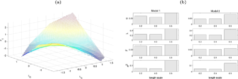
Figure 1: Panel (a): true interaction effect in all simulations. Panel (b): statistic AAD, (D.1) in Section D of Mayrink and Lucas (2013), and the comparison of models 1 and 2 with different choices of $l_{s}$ (simulation 1).

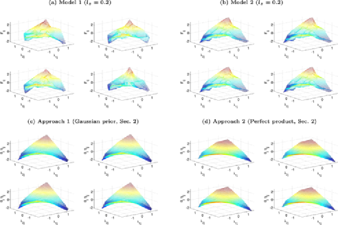
Figure 2: 3-D surface plot representing the estimated interaction effect.

The model with multiplicative interactions (1) can be compared with model (4) in Section 3. The interaction effect $\theta_{i\cdot}\eta$ corresponds to $F_{i\cdot}$. Note that $\theta_{i\cdot}=\mathbf{0}$ represents $F_{i\cdot}=\mathbf{0}$. In terms of prior specifications, initial values and MCMC configuration, consider the same choices defined in the simulated studies developed in Sections B and D of Mayrink and Lucas (2013). In this section, we concentrate on the comparison of surface plots to see how well the saddle shape in Figure 1 is estimated. Figure 2 shows the surfaces indicating the estimated interaction effect; we can identify the saddle shape in all cases. As one might expect, the multiplicative model [panels (c) and (d)] produces a smoother surface than the nonlinear model [panels (a) and (b)]. The multiplicative model is in advantage, because it assumes the true saddle shape as the target effect. The parameter $l_{s}$ can be used to control the smoothness of the surface in the nonlinear model (current choice $l_{s}=0.2$). If this value is increased, the number of neighbors influencing each point increases; the covariance matrix is then more populated. Figure 3 presents the surfaces related to models 1 and 2 assuming bigger choices of $l_{s}$. As can be seen, the level of irregularities in the middle of the graph seems reduced with respect to $l_{s}=0.2$; this conclusion is more evident for model 1 with $l_{s}=0.5$.

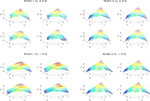
Figure 3: 3-D surface plot representing the estimated interaction effect ($l_{s}=0.3$ or 0.5).

The smooth surfaces, for $l_{s}=0.5$ in Figure 3, seem to be flatter and wider than the other cases. This characteristic can be interpreted as an indication of worse approximation between posterior estimates and true values. The bar plots in Figure 1(b) compare the AAD statistic, (D.1) in Section D of Mayrink and Lucas (2013), for parameters in models 1 and 2 with different choices of $l_{s}$. Note that the approximation is indeed worse when $l_{s}=0.5$; the biggest AAD value is observed for $l_{s}=0.5$ in all cases.

Applications involving other data sets (simulations 2 and 3) and other models (models 3, 4 and 5) provide the same conclusions above.

5 Real application: CNA and multiplicative interactions

The number of copies of a gene in a chromosome can be modified as a consequence of problems during cell division and these alterations are known to play an important role in human cancer. We wish to examine the possibility that there are genes that are synergistically affected by copy number alteration in multiple genomic locations. In order to assess this, we will build factor models in which we seed each latent factor with a set of genes that is known to be in a single region of copy number alteration (CNA). We accomplish the seeding with the prior assumption that they have nonzero factor loadings on the factor with very high probability. We then utilize our interaction model to assess all genes for interaction effects between two copy number alteration factors. Positive results will indicate genes that are synergistically differentially expressed in the presence of multiple CNAs and may lead to insights about the mechanism of action of the CNAs.

Many studies have detected CNA in breast cancer data, for example, Pollack et al. (2002), Przybytkowski, Ferrario and Basik (2011) and Lucas, Kung and Chi (2010). In our analyses, different regions of CNA are drawn from Lucas, Kung and Chi (2010). Each region is an interval, involving a collection of genes, located in the human genome sequence. The locations suggesting CNA are known, and an annotation file identifying the chromosome position for each probe set can be obtained from the Affymetrix website. In order to identify our seed genes, we consider a range (2,000,000 to the left and right) around the central position where the CNA seems to occur. We explore four different breast cancer data sets: Chin et al. (2006), Miller et al. (2005), Sotiriou et al. (2006) and Wang et al. (2005).

We investigate the results for two groups of over-expressed genes. The first one has central position 35,152,961 in chromosome 22; we denote this group as $G_{1}$. The second collection of genes is located around the central point 68,771,985 in chromosome 16; let $G_{2}$ represent this group. We will fit a factor model with $L=2$ latent factors describing the expression pattern of the genes in $G_{1}$ and $G_{2}$. The model includes a third factor representing the multiplicative interaction between the first two. Our goal is to identify the genes affected by the interaction factor.

The group $G_{1}$ has 50 genes, and $G_{2}$ contains 42 elements. As described above, the selection of these genes is based on an interval specified around a position in the genome. This strategy can lead to the inclusion of cases unrelated to the CNA detected for the studied region. In order to remove the unrelated cases from the current gene lists, we fit a two-factor model (without interaction terms) to the ($92\times n$) matrix $X$. The following configuration is expected for the estimated $\alpha\dvtx\{\alpha_{i1}\dvtx i\in G_{1}\}$ with the same sign, $\{\alpha_{i2}\dvtx i\in G_{2}\}$ with the same sign, and $\alpha_{il}=0$ for all other cases. The genes in $(G_{1}\cup G_{2})$ violating this assumption are considered problematic, and thus removed from the analysis. This cleaning procedure involving $G_{1}$ and $G_{2}$ is described with more details in Section E of Mayrink and Lucas (2013). The procedure defines 22 genes in $G_{1}$ and 18 in $G_{2}$.

Let $G_{E}$ represent a group of extra genes to be included in the analysis; $G_{1}$, $G_{2}$ and $G_{E}$ are disjoint sets. The microarrays selected for this application have 22,283 genes, and each breast cancer data set has more than 100 samples available for analysis. As a result, the MCMC algorithm can be rather slow to handle this large amount of data. As an alternative to reduce the computational cost, we implement a gene selection procedure to eliminate the cases which might not be affected by interactions. The full description of the selection process is given in Section E of Mayrink and Lucas (2013). In short, we fit a two-factor model (without interaction terms) to the ($22\mbox{,}283\times n$) matrix $X$ assuming 22 genes in $G_{1}$, 18 genes in $G_{2}$ and 22,243 genes in $G_{E}$. The distribution of the conditional probability $p(h_{il}=1|\cdots)$ is evaluated to accept or reject $\alpha_{il}\neq 0$. It seems reasonable to assume that the genes affected by both factors are more likely to be affected by interactions, therefore, the final result includes only the cases satisfying this requirement. This selection process yields 3704 genes in the updated $G_{E}$.

Consider the prior specifications: $\omega_{\alpha}=\omega_{\theta}=10$ in (2) and (2), $\sigma^{2}_{i}\sim\mathit{IG}(2.1,\allowbreak 1.1)$. Our goal is to fit the factor model with multiplicative interaction effects (using approach 1${}={}$Gaussian prior) to the real data having 22 genes in $G_{1}$, 18 genes in $G_{2}$ and 3704 genes in $G_{E}$. Given the large amount of genes, we need to set strong priors for $q_{il}$ to impose our assumptions related to $G_{1}$ and $G_{2}$ and assure the identification of the model. We use the configuration indicated as “option 2” in Table B.1. Degenerated priors are assumed to impose our assumptions regarding the gene–factor relationship for the cases in $G_{1}$ and $G_{2}$. This strategy is important to retain the CNA interpretation of factors 1 and 2; otherwise, the target association can be overwhelmed by the large amount of information in $G_{E}$. Note that we assume no interaction affecting the genes in ($G_{1}\cup G_{2}$). The Beta($1,10$) is specified to induce sparsity in the loadings ($i\in G_{E}$) related to the interaction factor. Finally, the $U(0,1)$ is indicated for all other cases.

The MCMC algorithm performs 600 iterations (burn-in period${}={}$400). In terms of initial values of the chains, consider the same choices defined in Section B of Mayrink and Lucas (2013) for $\alpha_{il}^{(0)}$, $\lambda_{lj}^{(0)}$, $\theta_{i}^{(0)}$, $\eta_{j}^{(0)}$ and $(\sigma^{2}_{i})^{(0)}$. The probabilities $q_{il}$ and $\rho_{i}$ are initialized with the values presented in Table B.1 (option 2); $h_{il}^{(0)}\sim\operatorname{Bernoulli}(q_{il}^{(0)})$ and $z_{i}^{(0)}\sim\operatorname{Bernoulli}(\rho_{i}^{(0)})$. The chains seem to converge in all applications of the MCMC algorithm.

The model assuming the prior $\eta_{j}\sim N(\lambda_{1j}\lambda_{2j},\nu)$ (approach 1) is the focus of the first application in the current section. As previously discussed, the variance parameter $\nu$ must be small to guarantee the target multiplicative effect. The real data set contains a large number of genes and, thus, the posterior variance is expected to be small. In this case, only extremely small values for $\nu$ will ensure that $\eta_{j}$ and $\lambda_{1j}\lambda_{2j}$ are correlated. Figure 4 shows scatter plots comparing the posterior estimates of $\eta_{j}$ and the product $\lambda_{1j}\lambda_{2j}$. Here, the factor model is fitted with $\nu=10^{-5}$. Note that the model fit for the data set “Sotiriou” is the only one indicating correlated results. In the other applications, the multiplicative effect is lost and the interaction factor is just another factor.

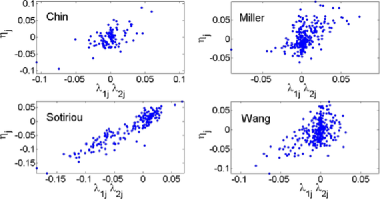
Figure 4: Scatter plots comparing the posterior estimates of $\eta_{j}$ and $\lambda_{1j}\lambda_{2j}$ (approach 1${}={}$Gaussian prior). Each panel represents a different breast cancer data set.

Given the difficulty to set $\nu$, no further real data analysis is developed for the factor model with approach 1. Our next step is to investigate the model defined as approach 2, where we force the perfect association $\eta_{j}=\lambda_{1j}\lambda_{2j}$. Consider the same breast cancer data sets, configuration of prior distributions, initial values and MCMC setup defined in the previous application. Because we impose the equality between $\eta_{j}$ and $\lambda_{1j}\lambda_{2j}$, the scatter plots comparing their values indicate correlation 1. Figure 5 shows the 95% credible interval and the posterior mean for $\alpha_{il}$ and $\theta_{i}$ such that $i\in(G_{1}\cup G_{2})$. Note that most nonzero loadings, related to the same factor, indicate posterior estimates with the same sign. This fact is observed for all data sets, and it supports the CNA interpretation for factors 1 and 2. Recall that the zero estimates are imposed via prior distribution to satisfy our assumptions for this group of genes.

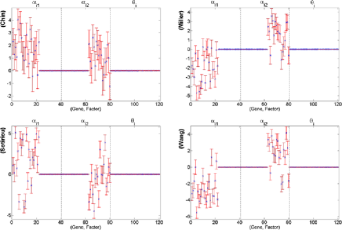
Figure 5: Posterior mean (x mark) and the 95% credible interval (bar) for the loadings with $i\in(G_{1}\cup G_{2})$ (approach 2${}={}$perfect product). Intervals are computed for the component with highest posterior probability weight. Dashed lines separate the factors.

Table 2 indicates (main diagonal) the number of genes affected by multiplicative interactions in each real data application. Note that the majority of features are free from interaction effects. The elements off diagonal are the number of common genes belonging to the intersection between the groups of affected genes. As can be seen, at least 14 genes can be found in the intersections involving different data sets. This result may be used as an argument against the idea that the model might be identifying interactions for a random set of genes. The intersections involving three data sets have 2–6 elements. Only 1 gene belongs to the intersection of all four data sets; its official full name is “GTP binding protein 4,” and it is located in chromosome 10.

=200pt Chin Miller Sotiriou Wang Chin 314 030 024 020 Miller 030 170 014 024 Sotiriou 024 014 244 024 Wang 020 024 024 255

Table 2: Pairwise intersections between data sets; number of common genes affected by the multiplicative interaction

We apply a hypothesis test to investigate whether the configuration in Table 2 can be considered a result of an independent random sample of genes, from the population of 3704 cases in $G_{E}$, for each breast cancer data set. First, we select genes, uniformly at random, using the numbers in the main diagonal of Table 2 as the sample sizes. In the next step, we consider the pairwise intersections between the random selections and obtain the sum of elements in all intersections; this number $n_{k}$ represents the level of overlaps. We repeat this procedure 100,000 times to generate $\{n_{k}\dvtx k=1,2,\ldots,100\mbox{,}000\}$. Finally, we calculate the number of cases such that $n_{k}\geq n_{\mathrm{o}}$, where $n_{\mathrm{o}}$ is the overlap level observed in Table 2. This result is then divided by 100,000 to provide the $p$-value 0.00003. In conclusion, we reject the hypothesis that the genes are independently selected for each data set.

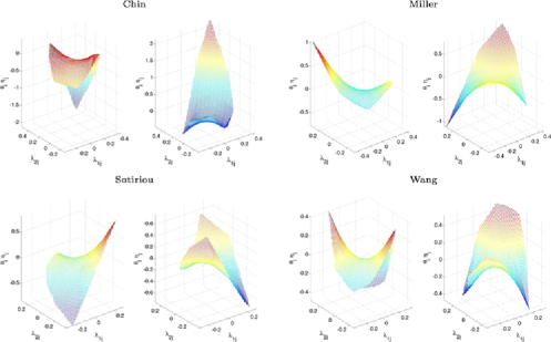
Figure 6: 3-D surface plots representing the multiplicative interaction effect $\theta_{i}\eta_{j}$ (approach 2${}={}$perfect product). In each panel, left${}={}$the smallest negative loading, and right${}={}$the largest positive loading.

Figure 6 shows the three-dimensional surface plot representing the multiplicative effect associated with the genes with the highest interaction effects. As can be seen, this type of interaction has a saddle shape. Each point in the surface corresponds to a different sample $j$. In the x and y axes we have $\lambda_{1j}$ and $\lambda_{2j}$; the z axis represents $\theta_{i}\eta_{j}$. The loading $\theta_{i}$ controls how strong the interaction effect is; values close to zero define flatter surfaces. The sign of $\theta_{i}$ determines the orientation of the saddle. In each panel, the graph on the left is related to the smallest negative $\theta_{i}$, while the graph on the right represents the largest positive $\theta_{i}$.

6 Real application: CNA and nonlinear interactions

Consider again the CNA problem investigated in the previous section using the four breast cancer data sets: Chin et al. (2006), Miller et al. (2005), Sotiriou et al. (2006) and Wang et al. (2005). Two latent factors are defined in our model for this type of application. In other words, $\lambda$ has two rows of factor scores, and each row describes the expression pattern across samples for the genes associated with a region where the CNA was detected. We will evaluate the model fit assuming three different pairs of chromosome locations. Table 3 identifies the position and chromosome number for each region. Denote by $G_{1}$ the group of genes around the first location in the pair; $G_{2}$ represents the collection of features around the second location. The cleaning procedure, described in Section E of Mayrink and Lucas (2013), is applied to remove problematic genes from $G_{1}$ and $G_{2}$. Table 3 indicates the number of genes before and after the removal procedure.

=270pt Number of genes Region Chr. Position Before After 1 11 117,844,879 38 13 2 22 035,152,961 50 22 3 07 101,400,207 45 24 4 16 068,771,985 42 18

Table 3: Regions detected with CNA. We apply a procedure to remove genes unrelated to the CNA factors. The number of genes before and after this removal is presented

The microarrays have 22,283 genes and each data set contains at least 118 samples. In order to reduce the computational cost, consider again the gene selection procedure described in Section E of Mayrink and Lucas (2013). The method is based on the data set in Chin et al. (2006), and we evaluate the pairs of regions $(1,4)$, $(2,4)$ and $(3,4)$; see Table 3. The selection indicates 3717, 3704 and 3708 elements in $G_{E}$ for the pairs $(1,4)$, $(2,4)$ and $(3,4)$. For the purpose of comparison, this configuration of $G_{E}$ is used to study all data sets. Our goal is to identify features in $G_{E}$ affected by interactions.

Model 1 in Table 1 is more convenient for applications with large $m$. In this case, we assume a particular Bernoulli probability for each indicator $h_{il}$ and $z_{i}$, which makes these variables less dependent on other observations. If a large number of $h_{il}$ share the same Bernoulli probability $q_{R}$, the level of sparsity in $\alpha$ can be incorrectly determined. If most loadings are nonzero values, $q_{R}$ tend to be large which favors $h_{il}=1$ for all $(i,l)$ related to $q_{R}$. Similarly, if a large number of $z_{i}$ share the same probability $\rho$ (models 3, 4) or $\rho_{R}$ (model 5), and if $F_{i\cdot}=\mathbf{0}$ for most genes, then $\rho$ or $\rho_{R}$ tend to be small which favors $z_{i}=0$ for all involved features. Here, the level of sparsity is too high and some interaction effects are neglected. In a real application, it seems more realistic to assume different interaction effects for different affected genes; for this reason, model 1 is preferred to model 2.

Assume $\omega=10$ in the mixture prior for $\alpha_{il}$, $\sigma^{2}_{i}\sim\mathit{IG}(2.1,1.1)$, and set $l_{s}=0.2$ in (5). The specifications in Table D.1 (option 2) are defined for $q_{il}$ and $\rho_{i}$ to impose our assumptions regarding the gene–factor relationship and provide the identification of the model. We do not expect interaction effects related to the genes in $G_{1}$ and $G_{2}$; these groups have a strong relationship with one latent factor and no association with the other. In addition, recall that most rows of $F$ should be null-vectors to ensure the identification between $\alpha\lambda$ and $F$. It is reasonable to expect few genes affected by interactions; as a result, one might choose a Beta distribution with higher probability mass below 0.5 for $\rho_{i}$ with $i\in G_{E}$. The choice $\rho_{i}\sim\operatorname{Beta}(1,1)$ works well in the applications of this section.

In terms of initial values of the chains, let $F_{ij}^{(0)}=0$ for all $(i,j)$, and consider the usual choices $\alpha_{il}^{(0)}=0$, $(\sigma^{2}_{i})^{(0)}=1$, and $\lambda_{lj}^{(0)}\sim N(0,1)$. We initialize $h_{il}^{(0)}\sim\operatorname{Bernoulli}(q_{il}^{(0)})$ and $z_{i}^{(0)}\sim\operatorname{Bernoulli}(\rho_{i}^{(0)})$, where $q_{il}^{(0)}$ and $\rho_{i}^{(0)}$ are indicated in Table D.1 (option 2). The MCMC algorithm is set to perform 600 iterations (burn-in period${}={}$300); the chains seem to converge in all applications. The Metropolis–Hastings algorithm, used to sample from the full conditional posterior distribution of $\lambda_{\cdot j}$, has acceptance rate around 31–40%, 15–65%, 26–53% and 67–84% in the applications related to the data sets [Chin et al. (2006), Miller et al. (2005), Sotiriou et al. (2006) and Wang et al. (2005)].

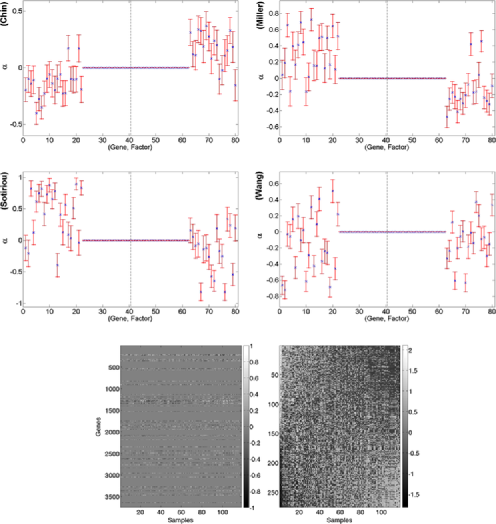
Figure 7: Results related to the pair of locations $(2,4)$. First four panels: posterior mean (x mark) and 95% credible interval (bar) for $\alpha_{il}$ with $i\in(G_{1}\cup G_{2})$; the dashed line separates the two factors. Fifth panel: left-hand side${}={}$full matrix $F$ (3744 genes), right-hand side${}={}$cases $F_{i\cdot}\neq 0$ (rows and columns are sorted so that the 1st principal components are monotone).

The 5th panel in Figure 7 shows images of interaction effects in $F$. The image on the left represents the full matrix with 3744 rows and 118 columns; the color bar is constrained between $(-1,1)$ for higher contrast. The second heat map exhibits the cases $F_{i\cdot}\neq 0$. Note that we identify 275 genes affected by nonlinear interactions involving the factors. Further, the second image suggests a coherent pattern for groups of features; several rows have similar decreasing or increasing effect, as we move across samples. This result supports the idea of $F_{i\cdot}$ as a representation of interactions; on the contrary, a random pattern would be observed for most rows. Figure 7 also presents the posterior estimates and 95% credible interval for the loadings related to genes in $G_{1}$ and $G_{2}$. These results are computed for the component in the posterior mixture with the highest probability weight. As can be seen, most intervals in $G_{l}$, $l=1$ or 2, suggest loadings with the same sign. This result supports the association between factors 1–2 and the CNA detected for $G_{1}$ and $G_{2}$. In other words, the estimated interactions seem to be a result of the CNA in regions 2 and 4.

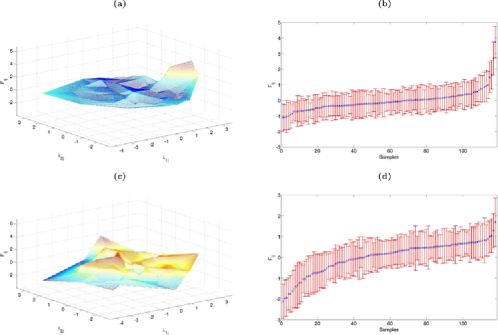
Figure 8: 3-D surface plot of the estimated interaction effect $F_{1524\cdot}$ (a) and $F_{1945\cdot}$ (c). Panels (b) and (d) contain the posterior mean (x mark) and the 95% credible interval (bar). This result is related to the data set Chin et al. (2006) and the pair of locations $(2,4)$.

Figure 8 shows, in panels (a) and (c), the three-dimensional surface plot representing the shape of the estimated interaction effect for two genes. The x and y axes contain the estimated $\lambda_{1j}$ and $\lambda_{2j}$, therefore, each point in the x–y plane is related to a sample (microarray). These shapes are different, suggesting distinct interaction effects for those genes. Panels (b) and (d) present the posterior mean used in the z axis of the graph and the corresponding 95% credible interval indicating our posterior uncertainty related to the estimated surface.

Table 4 compares the list of affected genes related to different breast cancer data sets. The table is divided in three sections representing the pair of regions with CNA. The main diagonal in each section indicates the number of affected genes. Note that all intersections are nonempty sets, that is, different data sets indicate the same group of genes as affected by interactions. Given the large number of genes in $G_{E}$ and the relatively small list of affected cases determined in each application, the identification of elements in the intersections is an important result suggesting a plausible model. Most intersections involving three data sets have 1 or 2 elements for any pair of regions.

=259pt Chin Miller Sotiriou Wang Pair $(1,4)$ Chin 139 006 008 009 Miller 006 081 006 003 Sotiriou 008 006 121 001 Wang 009 003 001 046 Pair $(2,4)$ Chin 275 014 013 019 Miller 014 111 007 007 Sotiriou 013 007 143 008 Wang 019 007 008 111 Pair $(3,4)$ Chin 235 010 011 007 Miller 010 091 004 009 Sotiriou 011 004 115 002 Wang 007 009 002 075

Table 4: Intersections between data sets; common genes affected by interactions

We evaluate the results of Table 4 to test the hypothesis of independent random samples of genes for each data set. This same test was used in Section 5 to examine Table 2. The configuration of Table 4 provides the $p$-values: 0.00002 for the pair $(1,4)$, 0.00001 for $(2,4)$ and 0.00044 for $(3,4)$. Assuming a significance level of 0.05, we reject the indicated null hypothesis.

In our final comparison analysis, the frameworks approach 1 (Section 2) and model 1 (Section 3) have been used to fit the data sets [Chin et al. (2006), Miller et al. (2005), Sotiriou et al. (2006) and Wang et al. (2005)]; consider the pair of regions $(2,4)$ in Table 3. Each model provides a list of genes affected by interactions; we have found 22 (Chin), 7 (Miller), 13 (Sotiriou) and 7 (Wang) genes in the intersection of the lists generated for the same data set. This type of result reinforces the idea that the proposed models can be valid to study interactions.

7 Conclusions

In an ordinary factor analysis, the involvement of any feature with the factors is always additive. Biological pathways establishing complex structure of dependencies between genes motivate the idea of a multi-factor model with interaction terms. We study the expression pattern across samples using Affymetrix GeneChip${}^{\bigcirc\texttt{\tiny R}}$ microarrays. The matrix $X$ contains the preprocessed data (RMA outputs) with rows representing genes and columns representing microarrays. Each column is a different individual, but all samples are related to the same type of cancer cell. We formulate the factor models with spike and slab prior distributions to allow for sparsity and then test whether the effect of factors/interactions on the features is significant or not. Simulated studies have been developed to verify the performance of the proposed models; the posterior estimates approximate well the real values.

In Section 2 we have proposed a model with pairwise multiplicative interactions, but any function defining a relationship between a pair of factors can be used. Two approaches were considered to introduce the interaction effect: (1) the product is inserted as the mean of a Gaussian prior, (2) we assume the perfect product between factors in a deterministic setup. In the real data application we have studied four breast cancer data sets. Two factors were defined in the model, and each one is directly associated with the genes located in a particular region (detected with CNA) of the human genome. The main aim was to identify other genes affected by the product interaction of the two factors. A selection process was implemented to choose the most interesting genes for this study, nevertheless, the matrix $X$ represents a large number of features. In this case, approach 1 requires a Gaussian prior with extremely small variance to ensure the multiplicative effect. On the other hand, approach 2 does not suffer from the same problem given its deterministic formulation. Depending on the data set, we have observed 170–314 genes affected by interactions, and the pairwise intersections of these groups have at least 14 elements.

In Section 3 we have developed a multi-factor model with a nonlinear structure of interactions; this version is more general. The nonlinearities involving the latent factors were introduced through the Squared Exponential kernel, which defines the covariance matrix in the Gaussian component of a mixture prior specified for the parameter representing interaction effects. One version of this prior assumes that the effect can be different comparing affected genes; the less realistic assumption “same effect for any pair of affected features” was also studied. In addition, different prior formulations were considered for probability parameters in the mixture prior specified for the interaction effects and for the factor loadings. As a result, five versions of the model were defined for investigation. Assumptions related to the intended type of application were used to choose the priors and induce a specific configuration in the matrices of factors loadings and interaction effects, which provides the identification of the model. In the real data application, we have revisited the two-factor analysis based on regions with CNA. Four breast cancer data sets were explored, and interactions can be identified in all evaluations. The intersections of results from the four data sets are nonempty sets which suggest a plausible model.

The use of a different covariance function can be an alternative to better combine smoothness and good posterior estimation. Of particular interest in this regard is the Matern class of covariance functions $K(r)=[2^{1-\upsilon}/\Gamma(\upsilon)](r\sqrt{2\upsilon}/l_{s})^{\upsilon}\*K_{\upsilon}(r\sqrt{2\upsilon}/l_{s})$ with positive parameters $\upsilon$ and $l_{s}$, where $K_{\upsilon}$ is a modified Bessel function [see Abramowitz and Stegun (1965), Section 9.6] and $r$ is the Euclidean length. The parameter $\upsilon$ is, in fact, a smoothness parameter. The Squared Exponential covariance function $\exp\{-r^{2}/(2l_{s}^{2})\}$ is obtained for $\upsilon=\infty$ [see Rasmussen and Williams (2006), page 204]. The process is $k$-times Mean Squared differentiable if and only if $\upsilon>k$. In summary, we currently control the range of influence between points using the parameter $l_{s}$. In order to improve smoothness and retain good posterior approximation, one could try to balance the choices of $l_{s}$ and $\upsilon<\infty$.

In Section 3 we have studied two mixture priors for $F_{i\cdot}$ specifying extreme cases, that is, the effects are all different or the same. It would be reasonable to consider the intermediate situation, where we identify groups of genes such that the nonlinear interaction is the same within each group, but it differs between groups. In order to implement this assumption, we can use the clustering properties of the Dirichlet Process (DP) [Ferguson (1973, 1974)]. The following result is implied by the Polya urn scheme in Blackwell and MacQueen (1973), and it leads to the so-called “Chinese Restaurant Process” [see Aldous (1985), page 92]: $(\psi_{i}|\psi_{1},\ldots,\psi_{i-1})\sim[\zeta/(\zeta+i-1)]P_{0}+\sum_{j=1}^{i-1}[1/(\zeta+i-1)]\delta_{\psi_{j}}$, where $\zeta$ is the concentration parameter and $P_{0}$ is the base distribution in the DP. This implies that the $i$th feature is drawn from a new cluster with probability proportional to $\zeta$ or is allocated to an existing cluster with probability proportional to the number of features in that cluster. As a result, we can consider the prior $(F_{i\cdot}^{\prime}|\lambda)\sim(1-\rho_{i})\delta_{0}(F_{i\cdot})+\rho_{i}DP(\zeta,P_{0})$ with $P_{0}=N_{n}[\mathbf{0},K(\lambda)]$, where $K(\lambda)$ is the covariance matrix depending on $\lambda$.

References

- Abramowitz and Stegun (1965) {bbook}[author] \bauthor\bsnmAbramowitz, \bfnmM\binitsM. and \bauthor\bsnmStegun, \bfnmI. A.\binitsI. A. (\byear1965). \btitleHandbook of Mathematical Functions. \bpublisherDover, \blocationNew York. \bptokimsref \endbibitem
- Aldous (1985) {bincollection}[mr] \bauthor\bsnmAldous, \bfnmDavid J.\binitsD. J. (\byear1985). \btitleExchangeability and related topics. In \bbooktitleÉcole D’été de Probabilités de Saint-Flour, XIII—1983. \bseriesLecture Notes in Math. \bvolume1117 \bpages1–198. \bpublisherSpringer, \blocationBerlin. \biddoi=10.1007/BFb0099421, mr=0883646 \bptokimsref \endbibitem
- Arminger and Muthen (1998) {barticle}[author] \bauthor\bsnmArminger, \bfnmG.\binitsG. and \bauthor\bsnmMuthen, \bfnmB. O.\binitsB. O. (\byear1998). \btitleA Bayesian approach to nonlinear latent variable models using the Gibbs Sampler and the Metropolis–Hastings algorithm. \bjournalPsychometrika \bvolume63 \bpages271–300. \bptokimsref \endbibitem
- Blackwell and MacQueen (1973) {barticle}[mr] \bauthor\bsnmBlackwell, \bfnmDavid\binitsD. and \bauthor\bsnmMacQueen, \bfnmJames B.\binitsJ. B. (\byear1973). \btitleFerguson distributions via Pólya urn schemes. \bjournalAnn. Statist. \bvolume1 \bpages353–355. \bidissn=0090-5364, mr=0362614 \bptokimsref \endbibitem
- Carvalho et al. (2008) {barticle}[mr] \bauthor\bsnmCarvalho, \bfnmCarlos M.\binitsC. M., \bauthor\bsnmChang, \bfnmJeffrey\binitsJ., \bauthor\bsnmLucas, \bfnmJoseph E.\binitsJ. E., \bauthor\bsnmNevins, \bfnmJoseph R.\binitsJ. R., \bauthor\bsnmWang, \bfnmQuanli\binitsQ. and \bauthor\bsnmWest, \bfnmMike\binitsM. (\byear2008). \btitleHigh-dimensional sparse factor modeling: Applications in gene expression genomics. \bjournalJ. Amer. Statist. Assoc. \bvolume103 \bpages1438–1456. \biddoi=10.1198/016214508000000869, issn=0162-1459, mr=2655722 \bptokimsref \endbibitem
- Chen et al. (2010) {barticle}[pbm] \bauthor\bsnmChen, \bfnmBo\binitsB., \bauthor\bsnmChen, \bfnmMinhua\binitsM., \bauthor\bsnmPaisley, \bfnmJohn\binitsJ., \bauthor\bsnmZaas, \bfnmAimee\binitsA., \bauthor\bsnmWoods, \bfnmChristopher\binitsC., \bauthor\bsnmGinsburg, \bfnmGeoffrey S.\binitsG. S., \bauthor\bsnmHero, \bfnmAlfred\binitsA., \bauthor\bsnmLucas, \bfnmJoseph\binitsJ., \bauthor\bsnmDunson, \bfnmDavid\binitsD. and \bauthor\bsnmCarin, \bfnmLawrence\binitsL. (\byear2010). \btitleBayesian inference of the number of factors in gene-expression analysis: Application to human virus challenge studies. \bjournalBMC Bioinformatics \bvolume11 \bpages552. \biddoi=10.1186/1471-2105-11-552, issn=1471-2105, pii=1471-2105-11-552, pmcid=3098097, pmid=21062443 \bptokimsref \endbibitem
- Chin et al. (2006) {barticle}[pbm] \bauthor\bsnmChin, \bfnmKoei\binitsK., \bauthor\bsnmDeVries, \bfnmSandy\binitsS., \bauthor\bsnmFridlyand, \bfnmJane\binitsJ., \bauthor\bsnmSpellman, \bfnmPaul T.\binitsP. T., \bauthor\bsnmRoydasgupta, \bfnmRitu\binitsR., \bauthor\bsnmKuo, \bfnmWen-Lin\binitsW.-L., \bauthor\bsnmLapuk, \bfnmAnna\binitsA., \bauthor\bsnmNeve, \bfnmRichard M.\binitsR. M., \bauthor\bsnmQian, \bfnmZuwei\binitsZ., \bauthor\bsnmRyder, \bfnmTom\binitsT., \bauthor\bsnmChen, \bfnmFanqing\binitsF., \bauthor\bsnmFeiler, \bfnmHeidi\binitsH., \bauthor\bsnmTokuyasu, \bfnmTaku\binitsT., \bauthor\bsnmKingsley, \bfnmChris\binitsC., \bauthor\bsnmDairkee, \bfnmShanaz\binitsS., \bauthor\bsnmMeng, \bfnmZhenhang\binitsZ., \bauthor\bsnmChew, \bfnmKaren\binitsK., \bauthor\bsnmPinkel, \bfnmDaniel\binitsD., \bauthor\bsnmJain, \bfnmAjay\binitsA., \bauthor\bsnmLjung, \bfnmBritt Marie\binitsB. M., \bauthor\bsnmEsserman, \bfnmLaura\binitsL., \bauthor\bsnmAlbertson, \bfnmDonna G.\binitsD. G., \bauthor\bsnmWaldman, \bfnmFrederic M.\binitsF. M. and \bauthor\bsnmGray, \bfnmJoe W.\binitsJ. W. (\byear2006). \btitleGenomic and transcriptional aberrations linked to breast cancer pathophysiologies. \bjournalCancer Cell \bvolume10 \bpages529–541. \biddoi=10.1016/j.ccr.2006.10.009, issn=1535-6108, pii=S1535-6108(06)00315-1, pmid=17157792 \bptokimsref \endbibitem
- DeSantis et al. (2009) {barticle}[mr] \bauthor\bsnmDeSantis, \bfnmStacia M.\binitsS. M., \bauthor\bsnmHouseman, \bfnmE. Andrés\binitsE. A., \bauthor\bsnmCoull, \bfnmBrent A.\binitsB. A., \bauthor\bsnmLouis, \bfnmDavid N.\binitsD. N., \bauthor\bsnmMohapatra, \bfnmGayatry\binitsG. and \bauthor\bsnmBetensky, \bfnmRebecca A.\binitsR. A. (\byear2009). \btitleA latent class model with hidden Markov dependence for array CGH data. \bjournalBiometrics \bvolume65 \bpages1296–1305. \biddoi=10.1111/j.1541-0420.2009.01226.x, issn=0006-341X, mr=2756518 \bptokimsref \endbibitem
- Ferguson (1973) {barticle}[mr] \bauthor\bsnmFerguson, \bfnmThomas S.\binitsT. S. (\byear1973). \btitleA Bayesian analysis of some nonparametric problems. \bjournalAnn. Statist. \bvolume1 \bpages209–230. \bidissn=0090-5364, mr=0350949 \bptokimsref \endbibitem
- Ferguson (1974) {barticle}[mr] \bauthor\bsnmFerguson, \bfnmThomas S.\binitsT. S. (\byear1974). \btitlePrior distributions on spaces of probability measures. \bjournalAnn. Statist. \bvolume2 \bpages615–629. \bidissn=0090-5364, mr=0438568 \bptokimsref \endbibitem
- Fridlyand et al. (2004) {barticle}[mr] \bauthor\bsnmFridlyand, \bfnmJane\binitsJ., \bauthor\bsnmSnijders, \bfnmAntoine M.\binitsA. M., \bauthor\bsnmPinkel, \bfnmDan\binitsD., \bauthor\bsnmAlbertson, \bfnmDonna G.\binitsD. G. and \bauthor\bsnmJain, \bfnmAjay N.\binitsA. N. (\byear2004). \btitleHidden Markov models approach to the analysis of array CGH data. \bjournalJ. Multivariate Anal. \bvolume90 \bpages132–153. \biddoi=10.1016/j.jmva.2004.02.008, issn=0047-259X, mr=2064939 \bptokimsref \endbibitem
- George and McCulloch (1993) {barticle}[author] \bauthor\bsnmGeorge, \bfnmE. I.\binitsE. I. and \bauthor\bsnmMcCulloch, \bfnmE.\binitsE. (\byear1993). \btitleVariable selection via Gibbs sampling. \bjournalJ. Amer. Statist. Assoc. \bvolume88 \bpages881–889. \bptokimsref \endbibitem
- George and McCulloch (1997) {barticle}[author] \bauthor\bsnmGeorge, \bfnmE. I.\binitsE. I. and \bauthor\bsnmMcCulloch, \bfnmE.\binitsE. (\byear1997). \btitleApproaches for Bayesian variable selection. \bjournalStatist. Sinica \bvolume7 \bpages339–373. \bptokimsref \endbibitem
- Geweke (1996) {bincollection}[mr] \bauthor\bsnmGeweke, \bfnmJ.\binitsJ. (\byear1996). \btitleVariable selection and model comparison in regression. In \bbooktitleBayesian Statistics, 5 (Alicante, 1994) \bpages609–620. \bpublisherOxford Univ. Press, \blocationNew York. \bidmr=1425430 \bptokimsref \endbibitem
- Henao and Winther (2010) {bmisc}[author] \bauthor\bsnmHenao, \bfnmR.\binitsR. and \bauthor\bsnmWinther, \bfnmO.\binitsO. (\byear2010). \bhowpublishedSparse linear identifiable multivariate modeling. Preprint, Cornell Univ, Ithaca, NY. Available at http://arxiv.org/abs/1004.5265. \bptokimsref \endbibitem
- Hoyer et al. (2009) {barticle}[author] \bauthor\bsnmHoyer, \bfnmP. O.\binitsP. O., \bauthor\bsnmJanzing, \bfnmD.\binitsD., \bauthor\bsnmMooij, \bfnmJ. M.\binitsJ. M., \bauthor\bsnmPeters, \bfnmJ.\binitsJ. and \bauthor\bsnmScholkopf, \bfnmB.\binitsB. (\byear2009). \btitleNonlinear causal discovery with additive noise models. \bjournalAdv. Neural Inf. Process. Syst. \bvolume21 \bpages689–696. \bptokimsref \endbibitem
- Lawrence (2004) {bincollection}[author] \bauthor\bsnmLawrence, \bfnmN. D.\binitsN. D. (\byear2004). \btitleGaussian process models for visualisation of high dimensional data. In \bbooktitleAdvances in Neural Information Processing Systems (\beditorS. Thrun, \beditorL. Saul and \beditorB. Scholkopf, eds.) \bvolume16 \bpages329–336. \bpublisherMIT Press, \blocationCambridge, MA. \bptokimsref \endbibitem
- Lawrence (2005) {barticle}[mr] \bauthor\bsnmLawrence, \bfnmNeil\binitsN. (\byear2005). \btitleProbabilistic non-linear principal component analysis with Gaussian process latent variable models. \bjournalJ. Mach. Learn. Res. \bvolume6 \bpages1783–1816. \bidissn=1532-4435, mr=2249872 \bptokimsref \endbibitem
- Lucas, Kung and Chi (2010) {barticle}[pbm] \bauthor\bsnmLucas, \bfnmJoseph E.\binitsJ. E., \bauthor\bsnmKung, \bfnmHsiu-Ni\binitsH.-N. and \bauthor\bsnmChi, \bfnmJen-Tsan A\binitsJ.-T. A. (\byear2010). \btitleLatent factor analysis to discover pathway-associated putative segmental aneuploidies in human cancers. \bjournalPLoS Comput. Biol. \bvolume6 \bpagese1000920. \biddoi=10.1371/journal.pcbi.1000920, issn=1553-7358, pmcid=2932681, pmid=20824128 \bptokimsref \endbibitem
- Lucas et al. (2006) {bincollection}[author] \bauthor\bsnmLucas, \bfnmJ. E.\binitsJ. E., \bauthor\bsnmCarvalho, \bfnmC.\binitsC., \bauthor\bsnmWang, \bfnmQ.\binitsQ., \bauthor\bsnmBild, \bfnmA.\binitsA., \bauthor\bsnmNevins, \bfnmJ. R.\binitsJ. R. and \bauthor\bsnmWest, \bfnmM.\binitsM. (\byear2006). \btitleSparse statistical modelling in gene expression genomics. In \bbooktitleBayesian Inference for Gene Expression and Proteomics (\beditorP. Muller, \beditorK. Do and \beditorM. Vannucci, eds.) \bpages155–176. \bpublisherCambridge Univ. Press, \blocationCambridge. \bptokimsref \endbibitem
- Marioni et al. (2006) {barticle}[author] \bauthor\bsnmMarioni, \bfnmJ. C.\binitsJ. C., \bauthor\bsnmThorne, \bfnmN. P.\binitsN. P., \bauthor\bsnmTavare, \bfnmS.\binitsS. and \bauthor\bsnmRadvanyi, \bfnmF.\binitsF. (\byear2006). \btitleBioHMM: A heterogeneous hidden Markov model for segmenting array CGH data. \bjournalBioinformatics \bvolume22 \bpages1144–1146. \bptokimsref \endbibitem
- Mayrink and Lucas (2013) {bmisc}[author] \bauthor\bsnmMayrink, \bfnmV. D.\binitsV. D. and \bauthor\bsnmLucas, \bfnmJ. E.\binitsJ. E. (\byear2013). \bhowpublishedSupplement to “Sparse latent factor models with interactions: Analysis of gene expression data.” DOI:\doiurl10.1214/12-AOAS607SUPP. \bptokimsref \endbibitem
- Miller et al. (2005) {barticle}[author] \bauthor\bsnmMiller, \bfnmL. D.\binitsL. D., \bauthor\bsnmSmeds, \bfnmJ.\binitsJ., \bauthor\bsnmGeorge, \bfnmJ.\binitsJ., \bauthor\bsnmVega, \bfnmV. B.\binitsV. B., \bauthor\bsnmVergara, \bfnmL.\binitsL., \bauthor\bsnmPloner, \bfnmA.\binitsA., \bauthor\bsnmPawitan, \bfnmY.\binitsY., \bauthor\bsnmHall, \bfnmP.\binitsP., \bauthor\bsnmKlaar, \bfnmS.\binitsS., \bauthor\bsnmLiu, \bfnmE. T.\binitsE. T. and \bauthor\bsnmBergh, \bfnmJ.\binitsJ. (\byear2005). \btitleAn expression signature for p53 status in human breast cancer predicts mutation status, transcriptional effects, and patient survival. \bjournalProc. Natl. Acad. Sci. USA \bvolume102 \bpages13550–13555. \bptokimsref \endbibitem
- Pollack et al. (2002) {barticle}[author] \bauthor\bsnmPollack, \bfnmJ. R.\binitsJ. R., \bauthor\bsnmSorlie, \bfnmT.\binitsT., \bauthor\bsnmPerou, \bfnmC. M.\binitsC. M., \bauthor\bsnmRees, \bfnmC. A.\binitsC. A., \bauthor\bsnmJeffrey, \bfnmS. S.\binitsS. S., \bauthor\bsnmLonning, \bfnmP. E.\binitsP. E., \bauthor\bsnmTibshirani, \bfnmR.\binitsR., \bauthor\bsnmBotstein, \bfnmD.\binitsD., \bauthor\bsnmDale, \bfnmA. L. B.\binitsA. L. B. and \bauthor\bsnmBrown, \bfnmP. O.\binitsP. O. (\byear2002). \btitleMicroarray analysis reveals a major direct role of DNA copy number alteration in the transcriptional program of human breast tumors. \bjournalProc. Natl. Acad. Sci. USA \bvolume99 \bpages12963–12968. \bptokimsref \endbibitem
- Przybytkowski, Ferrario and Basik (2011) {barticle}[pbm] \bauthor\bsnmPrzybytkowski, \bfnmEwa\binitsE., \bauthor\bsnmFerrario, \bfnmCristiano\binitsC. and \bauthor\bsnmBasik, \bfnmMark\binitsM. (\byear2011). \btitleThe use of ultra-dense array CGH analysis for the discovery of micro-copy number alterations and gene fusions in the cancer genome. \bjournalBMC Med. Genomics \bvolume4 \bpages16. \biddoi=10.1186/1755-8794-4-16, issn=1755-8794, pii=1755-8794-4-16, pmcid=3041991, pmid=21272361 \bptokimsref \endbibitem
- Rasmussen and Williams (2006) {bbook}[mr] \bauthor\bsnmRasmussen, \bfnmCarl Edward\binitsC. E. and \bauthor\bsnmWilliams, \bfnmChristopher K. I.\binitsC. K. I. (\byear2006). \btitleGaussian Processes for Machine Learning. \bpublisherMIT Press, \blocationCambridge, MA. \bidmr=2514435 \bptokimsref \endbibitem
- Sotiriou et al. (2006) {barticle}[author] \bauthor\bsnmSotiriou, \bfnmC.\binitsC., \bauthor\bsnmWirapati, \bfnmP.\binitsP., \bauthor\bsnmLoi, \bfnmS.\binitsS., \bauthor\bsnmHarris, \bfnmA.\binitsA., \bauthor\bsnmFox, \bfnmS.\binitsS., \bauthor\bsnmSmeds, \bfnmJ.\binitsJ., \bauthor\bsnmNordgren, \bfnmH.\binitsH., \bauthor\bsnmFarmer, \bfnmP.\binitsP., \bauthor\bsnmPraz, \bfnmV.\binitsV., \bauthor\bsnmKains, \bfnmB. H.\binitsB. H., \bauthor\bsnmDesmedt, \bfnmC.\binitsC., \bauthor\bsnmLarsimont, \bfnmD.\binitsD., \bauthor\bsnmCardoso, \bfnmF.\binitsF., \bauthor\bsnmPeterse, \bfnmH.\binitsH., \bauthor\bsnmNuyten, \bfnmD.\binitsD., \bauthor\bsnmBuyse, \bfnmM.\binitsM., \bauthor\bsnmVijver, \bfnmM. J. V. D.\binitsM. J. V. D., \bauthor\bsnmBergh, \bfnmJ.\binitsJ., \bauthor\bsnmPiccart, \bfnmM.\binitsM. and \bauthor\bsnmDelorenzi, \bfnmM.\binitsM. (\byear2006). \btitleGene expression profiling in breast cancer: Understanding the molecular basis of histologic grade to improve prognosis. \bjournalJournal of the National Cancer Institute \bvolume98 \bpages262–272. \bptokimsref \endbibitem
- Teh, Seeger and Jordan (2005) {bmisc}[author] \bauthor\bsnmTeh, \bfnmY. W.\binitsY. W., \bauthor\bsnmSeeger, \bfnmM.\binitsM. and \bauthor\bsnmJordan, \bfnmM. I.\binitsM. I. (\byear2005). \bhowpublishedSemiparametric latent factor models. In Proceedings of the Tenth International Workshop on Artificial Intelligence and Statistics (Z. Ghahramani and R. Cowell, eds.) 333–340. The Society for Artificial Intelligence and Statistics. \bptokimsref \endbibitem
- Titsias, Lawrence and Rattray (2009) {bincollection}[author] \bauthor\bsnmTitsias, \bfnmM.\binitsM., \bauthor\bsnmLawrence, \bfnmN. D.\binitsN. D. and \bauthor\bsnmRattray, \bfnmM.\binitsM. (\byear2009). \btitleEfficient sampling for Gaussian process inference using control variables. In \bbooktitleAdvances in Neural Information Processing Systems 21 (\beditorD. Koller, \beditorY. Bengio, \beditorD. Schuurmans and \beditorL. Bottou, eds.) \bpages689–696. \bpublisherMIT Press, \blocationCambridge, MA. \bptokimsref \endbibitem
- Wang et al. (2005) {barticle}[author] \bauthor\bsnmWang, \bfnmY.\binitsY., \bauthor\bsnmKlijn, \bfnmJ. G. M.\binitsJ. G. M., \bauthor\bsnmZhang, \bfnmY.\binitsY., \bauthor\bsnmSieuwerts, \bfnmA. M.\binitsA. M., \bauthor\bsnmLook, \bfnmM. P.\binitsM. P., \bauthor\bsnmYang, \bfnmF.\binitsF., \bauthor\bsnmTalantov, \bfnmD.\binitsD., \bauthor\bsnmTimmermans, \bfnmM.\binitsM., \bauthor\bsnmGelder, \bfnmM. E. M. V.\binitsM. E. M. V., \bauthor\bsnmYu, \bfnmJ.\binitsJ., \bauthor\bsnmJatkoe, \bfnmT.\binitsT., \bauthor\bsnmBerns, \bfnmE. M. J. J.\binitsE. M. J. J., \bauthor\bsnmAtkins, \bfnmD.\binitsD. and \bauthor\bsnmFoekens, \bfnmJ. A.\binitsJ. A. (\byear2005). \btitleGene expression profiles to predict distant metastasis of lymph-node-negative primary breast cancer. \bjournalLancet \bvolume365 \bpages671–679. \bptokimsref \endbibitem
- West (2003) {bincollection}[author] \bauthor\bsnmWest, \bfnmM.\binitsM. (\byear2003). \btitleBayesian factor regression models in the large , small paradigm. In \bbooktitleBayesian Statistics 7 (\beditorJ. Bernardo, \beditorM. Bayarri, \beditorJ. Berger, \beditorA. Dawid, \beditorD. Heckerman, \beditorA. Smith and \beditorM. West, eds.) \bpages723–732. \bpublisherOxford Univ. Press, \blocationOxford. \bptokimsref \endbibitem