SISSA 56/2013/FISI

RM3-TH/13-10

TTP13-04

Generalised Geometrical CP Violation
in a $\boldsymbol{T^{\prime}}$ Lepton Flavour Model

Ivan Girardi${}^{\,a,}$ , Aurora Meroni${}^{\,a,b,}$ , S. T. Petcov${}^{\,a,c,}$ , Martin Spinrath${}^{\,a,d,}$

^a SISSA/INFN, Via Bonomea 265, I-34136 Trieste, Italy

^b Dipartimento di Matematica e Fisica, Università di Roma Tre,

Via della Vasca Navale 84, I-00146 Rome, and

INFN, Laboratori Nazionali di Frascati, Via E. Fermi 40, I-00044 Frascati, Italy

^c Kavli IPMU (WPI), University of Tokyo, Tokyo, Japan

^d Institut für Theoretische Teilchenphysik, Karlsruhe Institute of Technology,

Engesserstraße 7, D-76131 Karlsruhe, Germany

We analyse the interplay of generalised CP transformations and the non-Abelian discrete group $T^{\prime}$ and use the semi-direct product $G_{f}=T^{\prime}\rtimes H_{\text{CP}}$, as family symmetry acting in the lepton sector. The family symmetry is shown to be spontaneously broken in a geometrical manner. In the resulting flavour model, naturally small Majorana neutrino masses for the light active neutrinos are obtained through the type I see-saw mechanism. The known masses of the charged leptons, lepton mixing angles and the two neutrino mass squared differences are reproduced by the model with a good accuracy. The model allows for two neutrino mass spectra with normal ordering (NO) and one with inverted ordering (IO). For each of the three spectra the absolute scale of neutrino masses is predicted with relatively small uncertainty. The value of the Dirac CP violation (CPV) phase $\delta$ in the lepton mixing matrix is predicted to be $\delta\cong\pi/2~{}{\rm or}~{}3\pi/2$. Thus, the CP violating effects in neutrino oscillations are predicted to be maximal (given the values of the neutrino mixing angles) and experimentally observable. We present also predictions for the sum of the neutrino masses, for the Majorana CPV phases and for the effective Majorana mass in neutrinoless double beta decay. The predictions of the model can be tested in a variety of ongoing and future planned neutrino experiments.

1 Introduction

Understanding the origin of the patterns of neutrino masses and mixing, emerging from the neutrino oscillation, ${}^{3}H$ $\beta-$decay, cosmological, etc. data is one of the most challenging problems in neutrino physics. It is part of the more general fundamental problem in particle physics of understanding the origins of flavour, i.e., of the patterns of the quark, charged lepton and neutrino masses and of the quark and lepton mixing.

At present we have compelling evidence for the existence of mixing of three light massive neutrinos $\nu_{i}$, $i=1,2,3$, in the weak charged lepton current (see, e.g., [1]). The masses $m_{i}$ of the three light neutrinos $\nu_{i}$ do not exceed approximately 1 eV, $m_{i}\ \raisebox{-1.72218pt}{\hbox to0.0pt{$\sim$\hss}}\raisebox{1.72218pt}{$<$}\ 1$ eV, i.e., they are much smaller than the masses of the charged leptons and quarks. The three light neutrino mixing is described (to a good approximation) by the Pontecorvo, Maki, Nakagawa, Sakata (PMNS) $3\times 3$ unitary mixing matrix, $U_{\rm PMNS}$. In the widely used standard parametrisation [1], $U_{\rm PMNS}$ is expressed in terms of the solar, atmospheric and reactor neutrino mixing angles $\theta_{12}$, $\theta_{23}$ and $\theta_{13}$, respectively, and one Dirac - $\delta$, and two Majorana [2] - $\beta_{1}$ and $\beta_{2}$, CP violation phases:

$$U_{\text{PMNS}}\equiv U=V(\theta_{12},\theta_{23},\theta_{13},\delta)\,Q(\beta_{1},\beta_{2})\,,$$ (1.1)

where

$$V=\begin{pmatrix}1&0&0\\ 0&c_{23}&s_{23}\\ 0&-s_{23}&c_{23}\\ \end{pmatrix}\begin{pmatrix}c_{13}&0&s_{13}e^{-\operatorname{\text{i}}\delta}\\ 0&1&0\\ -s_{13}e^{\operatorname{\text{i}}\delta}&0&c_{13}\\ \end{pmatrix}\begin{pmatrix}c_{12}&s_{12}&0\\ -s_{12}&c_{12}&0\\ 0&0&1\\ \end{pmatrix}\,,$$ (1.2)

and we have used the standard notation $c_{ij}\equiv\cos\theta_{ij}$, $s_{ij}\equiv\sin\theta_{ij}$, $0\leq\theta_{ij}\leq\pi/2$, $0\leq\delta\leq 2\pi$. The matrix $Q$ contains the two physical Majorana CP violation (CPV) phases:

$$Q=\operatorname{Diag}(\text{e}^{-\operatorname{\text{i}}\beta_{1}/2},\text{e}^{-\operatorname{\text{i}}\beta_{2}/2},1)\,.$$ (1.3)

The parametrization of the phase matrix $Q$ in Eq. (1.3) differs from the standard one [1] $Q=\operatorname{Diag}(1,\text{e}^{\operatorname{\text{i}}\alpha_{21}/2},\text{e}^{\operatorname{\text{i}}\alpha_{31}/2})$. Obviously, one has $\alpha_{21}=(\beta_{1}-\beta_{2})$ and $\alpha_{31}=\beta_{1}$. In the case of the seesaw mechanism of neutrino mass generation, which we are going to employ, the Majorana phases $\beta_{1}$ and $\beta_{2}$ (or $\alpha_{21}$ and $\alpha_{31}$) vary in the interval [3] $0\leq\beta_{1,2}\leq 4\pi$  . If CP invariance holds, we have $\delta=0,\pi,2\pi$, and [5] $\beta_{1(2)}=k^{(^{\prime})}\,\pi$, $k^{(^{\prime})}=0,1,2,3,4$.

All compelling neutrino oscillation data can be described within the indicated 3-flavour neutrino mixing scheme. These data allowed to determine the angles $\theta_{12}$, $\theta_{23}$ and $\theta_{13}$ and the two neutrino mass squared differences $\Delta m^{2}_{21}$ and $\Delta m^{2}_{31}$ (or $\Delta m^{2}_{32}$), which drive the observed oscillations involving the three active flavour neutrinos and antineutrinos, $\nu_{l}$ and $\bar{\nu}_{l}$, $l=e,\mu,\tau$, with a relatively high precision [6, 7]. In Table 1 we give the values of the 3-flavour neutrino oscillation parameters as determined in the global analysis performed in [6].

Parameter	best-fit ($\pm 1\sigma$)	3$\sigma$
$\Delta m^{2}_{21}\;[10^{-5}\text{ eV}^{2}]$	7.54${}^{+0.26}_{-0.22}$	6.99 - 8.18
$|\Delta m^{2}_{31}|~{}\text{ (NO)}\;[10^{-3}\text{ eV}^{2}]$	2.47${}^{+0.06}_{-0.10}$	2.19 - 2.62
$|\Delta m^{2}_{32}|~{}\text{ (IO)}\;[10^{-3}\text{ eV}^{2}]$	2.46${}^{+0.07}_{-0.11}$	2.17 - 2.61
$\sin^{2}\theta_{12}$ (NO or IO)	0.307${}^{+0.018}_{-0.016}$	0.259 - 0.359
$\sin^{2}\theta_{23}$ (NO)	0.386${}^{+0.024}_{-0.021}$	0.331 - 0.637
$\sin^{2}\theta_{23}$ (IO)	0.392${}^{+0.039}_{-0.022}$	0.335 - 0.663
$\sin^{2}\theta_{13}$ (NO)	0.0241${}^{+0.0025}_{-0.0025}$	0.0169 - 0.0313
$\sin^{2}\theta_{13}$ (IO)	0.0244${}^{+0.0023}_{-0.0025}$	0.0171 - 0.0315

Table 1: The best-fit values and $3\sigma$ allowed ranges of the 3-flavour neutrino oscillation parameters derived from a global fit of the current neutrino oscillation data (from [6]). If two values are given, the upper one corresponds to neutrino mass spectrum with normal hierarchy (NO) and the lower one - to spectrum with inverted hierarchy (IO) (see text for further details).

An inspection of Table 1 shows that although $\theta_{13}\neq 0$, $\theta_{23}\neq\pi/4$ and $\theta_{12}\neq\pi/4$, the deviations from these values are small, in fact we have $\sin\theta_{13}\cong 0.16\ll 1$, $\pi/4-\theta_{23}\cong 0.11$ and $\pi/4-\theta_{12}\cong 0.20$, where we have used the relevant best fit values in Table 1. The value of $\theta_{13}$ and the magnitude of deviations of $\theta_{23}$ and $\theta_{12}$ from $\pi/4$ suggest that the observed values of $\theta_{13}$, $\theta_{23}$ and $\theta_{12}$ might originate from certain “symmetry” values which undergo relatively small (perturbative) corrections as a result of the corresponding symmetry breaking. This idea was and continues to be widely explored in attempts to understand the pattern of mixing in the lepton sector (see, e.g., [8, 9, 10, 11, 12, 13, 14, 15, 16]). Given the fact that the PMNS matrix is a product of two unitary matrices,

$$U=U_{e}^{\dagger}\,U_{\nu}\,,$$ (1.4)

where $U_{e}$ and $U_{\nu}$ result respectively from the diagonalisation of the charged lepton and neutrino mass matrices, it is usually assumed that $U_{\nu}$ has a specific form dictated by a symmetry which fixes the values of the three mixing angles in $U_{\nu}$ that would differ, in general, by perturbative corrections from those measured in the PMNS matrix, while $U_{e}$ (and symmetry breaking effects that we assume to be subleading) provide the requisite corrections. A variety of potential “symmetry” forms of $U_{\nu}$, have been explored in the literature on the subject (see, e.g., [17]). Many of the phenomenologically acceptable “symmetry” forms of $U_{\nu}$, as the tribimaximal (TBM) [18] and bimaximal (BM) [19, 20] mixing, can be obtained using discrete flavour symmetries (see, e.g., the reviews [21, 22, 23] and the references quoted there in). Discrete symmetries combined with GUT symmetries have been used also in attempts to construct realistic unified models of flavour (see, e.g., [21]).

In the present article we will exploit the approximate flavour symmetry based on the group $T^{\prime}$, which is the double covering of the better known group $A_{4}$ (see, e.g., [23]), with the aim to explain the observed pattern of lepton (neutrino) mixing and to obtain predictions for the CP violating phases in the PMNS matrix and possibly for the absolute neutrino mass scale and the type of the neutrino mass spectrum. Flavour models based on the discrete symmetry $T^{\prime}$ have been proposed by a number of authors [24, 25, 26] before the angle $\theta_{13}$ was determined with a high precision in the Day Bay [27] and RENO [28] experiments (see also [29, 30, 31]). All these models predicted values of $\theta_{13}$ which turned out to be much smaller than the experimentally determined value.

In [25, 26], in particular, an attempt was made to construct a realistic unified supersymmetric model of flavour, based on the group $SU(5)\times T^{\prime}$, which describes the quark masses, the quark mixing and CP violation in the quark sector, the charged lepton masses and the known mixing angles in the lepton sector, and predicts the angle $\theta_{13}$ and possibly the neutrino masses and the type of the neutrino mass spectrum as well as the values of the CPV phases in the PMNS matrix. The light neutrino masses are generated in the model by the type I seesaw mechanism [32] and are naturally small. It was suggested in [25, 26] that the complex Clebsch-Gordan (CG) coefficients of $T^{\prime}$ [33] might be a source of CP violation and hence that the CP symmetry might be broken geometrically [34] in models with approximate $T^{\prime}$ symmetry. Since the phases of the CG coefficients of $T^{\prime}$ are fixed, this leads to specific predictions for the CPV phases in the quark and lepton mixing matrices. Apart from the incorrect prediction for $\theta_{13}$, the authors of [25, 26] did not address the problem of vacuum alignment of the flavon vevs, i.e., of demonstrating that the flavon vevs, needed for the correct description of the quark and lepton masses and of the the mixing in both the quark and lepton sectors, can be derived from a flavon potential and that the latter does not lead to additional arbitrary flavon vev phases which would destroy the predictivity, e.g., of the leptonic CP violation of the model.

A SUSY $SU(5)\times T^{\prime}$ model of flavour, which reproduces the correct value of the lepton mixing angle $\theta_{13}$ was proposed in [35], where the problem of vacuum alignment of the flavon vevs was also successfully addressed . In [35] it was assumed that the CP violation in the quark and lepton sectors originates from the complexity of the CG coefficients of $T^{\prime}$. This was possible by fixing the phases of the flavon vevs using the method of the so-called “discrete vacuum alignment”, which was advocated in [37] and used in a variety of other models with discrete flavour symmetries [38]. The value of the angle $\theta_{13}$ was generated by charged lepton corrections to the TBM mixing using non-standard GUT relations [13, 39, 40].

After the publication of [35] it was realised in [41, 42] that the requirement of CP invariance in the context of theories with discrete flavour symmetries, imposed before the breaking of the discrete symmetry leading to CP nonconservation and generation of the masses of the matter fields of the theory, requires the introduction of the so-called “generalised CP transformations” of the matter fields charged under the discrete symmetry. The explicit form of the generalised CP transformations is dictated by the type of the discrete symmetry. It was noticed in [41], in particular, that due to a subtle intimate relation between CP symmetry and certain discrete family symmetries, like the one associated with the group $T^{\prime}$, it can happen that the CP symmetry does not enforce the Yukawa type couplings, which generate the matter field mass matrices after the symmetry breaking, to be real but to have certain discrete phases predicted by the family symmetry in combination with the generalised CP transformations. In the $SU(5)\times T^{\prime}$ model proposed in [35], these phases, in principle, can change or modify completely the pattern of CP violation obtained by exploiting the complexity of some of the $T^{\prime}$ CG coefficients.

In the present article we address the problem of the relation between the $T^{\prime}$ symmetry and the CP symmetry in models of lepton flavour. After some general remarks about the connection between the $T^{\prime}$ and CP symmetries in Section 2, we present in Section 3 a fully consistent and explicit model of lepton flavour with a $T^{\prime}$ family symmetry and geometrical CP violation. We show that the model reproduces correctly the charged lepton masses, all leptonic mixing angles and neutrino mass squared differences and predicts the values of the leptonic CP violating phases and the neutrino mass spectrum. We show also that this model indeed exhibits geometrical CP violation. We clarify how the CP symmetry is broken in the model by using the explicit form of the constructed flavon vacuum alignment sector; without the knowledge of the flavon potential it is impossible to make conclusions about the origin of CP symmetry breaking in flavour models with $T^{\prime}$ symmetry. In the Appendix we give some technical details about the group $T^{\prime}$ and present a “UV completion” of the model, which is necessary in order to to select correctly certain $T^{\prime}$ contractions in the relevant effective operators.

2 $\boldsymbol{T^{\prime}}$ Symmetry and Generalised CP Transformations

In this Section we would like to clarify the role of a generalised CP transformation combined with the non-Abelian discrete symmetry group $T^{\prime}$. Let $G_{f}=T^{\prime}\rtimes H_{\text{CP}}$ be the symmetry group acting in the lepton sector such that both $T^{\prime}$ and $H_{\text{CP}}$ act on the lepton flavour space. Motivated by this study we will present in the next section a model where $G_{f}$ is broken such that all lepton mixing angles and physical CP phases of the PMNS mixing matrix can be predicted in terms of two mixing angles and two phases. The breaking of $G_{f}$ will be achieved through non zero vacuum expectation values (vevs) of some scalar fields, the so-called flavons.

2.1 The consistency conditions

The discrete non-Abelian family symmetry group $T^{\prime}$ is the double covering of the tetrahedral group $A_{4}$ and its complete description in terms of generators, elements and representations is given in Appendix A. An interesting feature of this group is the fact that it is the smallest group that admits 1-, 2-, and 3-dimensional representations and for which the three representations can be related by the multiplication rule $\textbf{2}\otimes\textbf{2}=\textbf{3}\oplus\textbf{1}$. $T^{\prime}$ has seven different irreducible representations: the 1- and 3-dimensional representations $\mathbf{1}$, $\mathbf{1}^{\prime}$, $\mathbf{1}^{\prime\prime}$, $\mathbf{3}$ are not faithful, i.e., not injective, while the doublet representations $\mathbf{2}$, $\mathbf{2}^{\prime}$ and $\mathbf{2}^{\prime\prime}$ are faithful. One interesting feature of the $T^{\prime}$ group is related to the tensor products involving the 2-dimensional representation since the CG coefficients are complex.

We define now the transformation of a field $\phi(x)$ under the group $T^{\prime}$ and $H_{\text{CP}}$ respectively as:

$$\phi(x)\rightarrow\rho_{r}(g)\phi(x),\qquad\phi(x)\rightarrow X_{r}\phi^{*}(x^{\prime}),$$ (2.1)

where $\rho_{r}(g)$ is an irreducible representation $r$ of the group element $g\in T^{\prime}$, $x^{\prime}\equiv(x^{0},-\vec{x})$ and $X_{r}$ is the unitary matrix representing the generalised CP transformation. In order to introduce consistently the CP transformation for the family symmetry group $T^{\prime}$, the matrix $X_{r}$ should satisfy the consistency conditions [41, 42, 44]:

$$X_{r}\rho_{r}^{*}(g)X_{r}^{-1}=\rho_{r}(g^{\prime})\,,\quad g,g^{\prime}\in T^{\prime}\,.$$ (2.2)

Following the discussion given in [41, 42, 44] it is important to remark that the consistency condition corresponds to a similarity transformation between the representation $\rho_{r}^{*}$ and $\rho\circ\text{CP}$. Since the structure of the group is preserved and an element $g\in T^{\prime}$ is always mapped into an element $g^{\prime}\in T^{\prime}$, this map defines an automorphism of the group. In general $g$ and $g^{\prime}$ might belong to different conjugacy classes: in this case the map defines an outer automorphism .

It is worth noticing that the matrices $X_{r}$ are defined up to an arbitrary global phase. Indeed, without loss of generality, for each matrix $X_{r}$, one can define different phases $\theta_{r}$ for different irreducible representations and moreover one can define $X_{r}$ up to a group transformation (change of basis): in fact the consistency conditions in Eq. (2.2) are invariant under $X_{r}\rightarrow\text{e}^{\operatorname{\text{i}}\theta_{r}}X_{r}$ and $X_{r}\rightarrow\rho_{r}(\tilde{g})X_{r}$ with $\tilde{g}\in T^{\prime}$.

It proves convenient to use the freedom associated with the arbitrary phases $\theta_{r}$ to define the generalised CP transformation for which the vev alignments of the flavon fields can be chosen to be all real. We will show later on that the phases $\theta_{r}$ are not physical and therefore the results we present are independent from the specific values we assume. In the context of the $T^{\prime}$ group this choice however helps us to extract a real flavon vev structure which is a distinctive feature of some models proposed in the literature where the origin of the physical CP violation arising in the lepton sector is tightly related to the combination of real vevs, complex CGs and eventual phases arising from the requirement of invariance of the superpotential under the generalised CP transformation.

Before going into details of the computations, let us comment that in the analysis presented in [41] related to the group $T^{\prime}$, the CP transformations are defined as elements of the outer automorphism group and are derived up to inner automorphisms of $T^{\prime}$ (up to conjugacy transformations). In the present work we will consider instead all the possible transformations including the inner automorphism group and we will discuss all the convenient CP transformations which can be used to clarify the role of a generalised CP symmetry in the context of the group $T^{\prime}$.

2.2 Transformation properties under generalised CP

We give now all the possible equivalent choices of generalised CP transformations for any irreducible representation of $T^{\prime}$.

The group $T^{\prime}$ is defined by the group generators $T$ and $S$, then from the consistency conditions in Eq. (2.2) it is sufficient to require that

$$X_{r}\rho_{r}^{*}(S)X_{r}^{-1}=\rho_{r}(\hat{S})\,,\qquad X_{r}\rho_{r}^{*}(T)X_{r}^{-1}=\rho_{r}(\hat{T})\,.$$ (2.3)

It is easy to show that the CP transformation leaves invariant the order of the element of the group $g$ meaning that denoting $n(g)$ the order of $g$, we have $n(g)=n(g^{\prime})$. Since the element $S$ has order four and the element $T$ has order three we have $\hat{S}\in 6\,C^{4}$ and $\hat{T}\in 4^{\prime}C^{3}$ [45]. The latter result is derived using the action of CP on the one-dimensional representations, i.e. $\rho_{1,1^{\prime},1^{\prime\prime}}(\hat{T})=\rho^{*}_{1,1^{\prime},1^{\prime\prime}}(T)$ which can be satisfied only if $\hat{T}\in 4^{\prime}C^{3}$.

The conjugacy classes $6\,C^{4}$ and $4^{\prime}C^{3}$ contain the group elements

$$\begin{split}\hat{S}\in 6\,C^{4}&=\left\{S,S^{3},TST^{2},T^{2}ST,S^{2}TST^{2},S^{2}T^{2}ST\right\}\,,\\ \hat{T}\in 4^{\prime}C^{3}&=\left\{T^{2},S^{2}TST,S^{2}T^{2}S,S^{3}T^{2}\right\}\,.\\ \end{split}$$ (2.4)

We recall that we have the freedom to choose arbitrary phases $\theta_{r}$, so for instance in the case of $X_{1}$, $X_{1^{\prime}}$ and $X_{1^{\prime\prime}}$ we are allowed to write the most general CP transformations for the three inequivalent singlets of $T^{\prime}$ as

$$\mathbf{1}\rightarrow\text{e}^{\operatorname{\text{i}}\theta_{1}}\mathbf{1}^{*}\;,\quad\mathbf{1^{\prime}}\rightarrow\text{e}^{\operatorname{\text{i}}\theta_{1^{\prime}}}\mathbf{1^{\prime}}^{*}\;,\quad\mathbf{1^{\prime\prime}}\rightarrow\text{e}^{\operatorname{\text{i}}\theta_{1^{\prime\prime}}}\mathbf{1^{\prime\prime}}^{*}\,.$$ (2.5)

Differently from the case of the $A_{4}$ family symmetry discussed in [44] in which one can show that the generalised CP transformation can be represented as a group transformation, in the case of $T^{\prime}$ we will show that this is true only for the singlet and the triplet representations. For the doublets the action of the CP transformation cannot be written as an action of a group element (i.e. $\nexists\,\,g\in T^{\prime}$ such that $X_{r}=\rho_{r}(g)$ for $r=\mathbf{2},\mathbf{2}^{\prime},\mathbf{2}^{\prime\prime}$).

We give a list of all the possible forms of $X_{r}$, which can be in general different for each representation: the CP transformations on the singlets, $X_{\mathbf{1},\mathbf{1}^{\prime},\mathbf{1}^{\prime\prime}}$, are complex phases, as mentioned above while the CP transformations on the doublets, $X_{\mathbf{2},\mathbf{2}^{\prime},\mathbf{2}^{\prime\prime}}$, and the triplets $X_{\mathbf{3}}$, are given respectively in Table 2 and 3. We stress that all the possible forms of $X_{r}$ are defined up to a phase, which can be in general different for each representation. Each CP transformation we found generates a $Z_{2}$ symmetry.

$g,g^{\prime}$	$X_{\mathbf{3}}=\rho_{3}(g)=\rho_{3}(g^{\prime})$	$T\rightarrow\hat{T}$	$S\rightarrow\hat{S}$
$T$, $S^{2}T$	$\left(\begin{array}[]{ccc}1&0&0\\ 0&\omega&0\\ 0&0&\omega^{2}\\ \end{array}\right)$	$T^{2}$	$S^{3}$
$T^{2}$, $S^{2}T^{2}$	$\left(\begin{array}[]{ccc}1&0&0\\ 0&\omega^{2}&0\\ 0&0&\omega\\ \end{array}\right)$	$T^{2}$	$S^{2}TST^{2}$
$E$, $S^{2}$	$\left(\begin{array}[]{ccc}1&0&0\\ 0&1&0\\ 0&0&1\\ \end{array}\right)$	$T^{2}$	$S^{2}T^{2}ST$
$TS$, $S^{2}TS$	$\left(\begin{array}[]{ccc}-1/3&2/3\,\omega&2/3\,\omega^{2}\\ 2/3&-1/3\,\omega&2/3\,\omega^{2}\\ 2/3&2/3\,\omega&-1/3\,\omega^{2}\\ \end{array}\right)$	$S^{2}T^{2}S$	$S$
$TST^{2}$, $S^{2}TST^{2}$	$\left(\begin{array}[]{ccc}-1/3&2/3&2/3\\ 2/3&-1/3&2/3\\ 2/3&2/3&-1/3\\ \end{array}\right)$	$S^{2}T^{2}S$	$T^{2}ST$
$S^{2}TST$, $TST$	$\left(\begin{array}[]{ccc}-1/3&2/3\,\omega^{2}&2/3\,\omega\\ 2/3&-1/3\,\omega^{2}&2/3\,\omega\\ 2/3&2/3\,\omega^{2}&-1/3\,\omega\\ \end{array}\right)$	$S^{2}T^{2}S$	$S^{2}TST^{2}$
$ST$, $S^{3}T$	$\left(\begin{array}[]{ccc}-1/3&2/3\,\omega^{2}&2/3\,\omega\\ 2/3\,\omega^{2}&-1/3\,\omega&2/3\\ 2/3\,\omega&2/3&-1/3\,\omega^{2}\\ \end{array}\right)$	$S^{2}TST$	$S^{3}$
$S^{3}T^{2}$, $ST^{2}$	$\left(\begin{array}[]{ccc}-1/3&2/3&2/3\\ 2/3\,\omega^{2}&-1/3\,\omega^{2}&2/3\,\omega^{2}\\ 2/3\,\omega&2/3\,\omega&-1/3\,\omega\\ \end{array}\right)$	$S^{2}TST$	$TST^{2}$
$S$, $S^{3}$	$\left(\begin{array}[]{ccc}-1/3&2/3\,\omega&2/3\,\omega^{2}\\ 2/3\,\omega^{2}&-1/3&2/3\,\omega\\ 2/3\,\omega&2/3\,\omega^{2}&-1/3\\ \end{array}\right)$	$S^{2}TST$	$T^{2}ST$
$S^{3}TS$, $STS$	$\frac{1}{9}\left(\begin{array}[]{ccc}4\omega^{2}+4\omega+1&-2\omega^{2}-2\omega+4&-2\omega^{2}-2\omega+4\\ -2\omega^{2}+4\omega-2&4\omega^{2}+\omega+4&-2\omega^{2}+4\omega-2\\ 4\omega^{2}-2\omega-2&4\omega^{2}-2\omega-2&\omega^{2}+4\omega+4\\ \end{array}\right)$	$S^{3}T^{2}$	$S$
$S^{2}T^{2}S$, $T^{2}S$	$\left(\begin{array}[]{ccc}-1/3&2/3\,\omega&2/3\,\omega^{2}\\ 2/3\,\omega&-1/3\,\omega^{2}&2/3\\ 2/3\,\omega^{2}&2/3&-1/3\,\omega\\ \end{array}\right)$	$S^{3}T^{2}$	$TST^{2}$
$T^{2}ST$, $S^{2}T^{2}ST$	$\left(\begin{array}[]{ccc}-1/3&2/3\,\omega^{2}&2/3\,\omega\\ 2/3\,\omega&-1/3&2/3\,\omega^{2}\\ 2/3\,\omega^{2}&2/3\,\omega&-1/3\\ \end{array}\right)$	$S^{3}T^{2}$	$S^{2}T^{2}ST$

Table 2: The generalised CP transformation for the triplet representation of the group $T^{\prime}$ derived using the consistency conditions. We have defined $\omega=\text{e}^{\operatorname{\text{i}}2\pi/3}$.

$X_{\mathbf{2}}$, $X_{\mathbf{2}^{\prime}}$, $X_{\mathbf{2}^{\prime\prime}}$	$T\rightarrow\hat{T}$	$S\rightarrow\hat{S}$		$X_{\mathbf{2}}$, $X_{\mathbf{2}^{\prime}}$, $X_{\mathbf{2}^{\prime\prime}}$	$T\rightarrow\hat{T}$	$S\rightarrow\hat{S}$
$\left(\begin{array}[]{cc}\bar{p}^{5}&0\\ 0&p^{5}\\ \end{array}\right)$	$T^{2}$	$S^{3}$		$\sqrt{\frac{2}{3}}\left(\begin{array}[]{cc}\bar{p}^{5}/\sqrt{2}&1\\ 1&\bar{p}^{7}/\sqrt{2}\\ \end{array}\right)$	$S^{2}TST$	$S^{3}$
$\left(\begin{array}[]{cc}\bar{p}&0\\ 0&p\\ \end{array}\right)$	$T^{2}$	$S^{2}TST^{2}$		$\frac{1}{\sqrt{3}}\left(\begin{array}[]{cc}p^{5}&\sqrt{2}q\\ \sqrt{2}q^{5}&\bar{p}^{5}\\ \end{array}\right)$	$S^{2}TST$	$TST^{2}$
$\left(\begin{array}[]{cc}e^{\operatorname{\text{i}}\pi/4}&0\\ 0&\text{e}^{-i\pi/4}\\ \end{array}\right)$	$T^{2}$	$S^{2}T^{2}ST$		$\left(\begin{array}[]{cc}e^{\operatorname{\text{i}}\pi/4}&\sqrt{2}q^{5}\\ \sqrt{2}q&\text{e}^{-i\pi/4}\\ \end{array}\right)$	$S^{2}TST$	$T^{2}ST$
$\left(\begin{array}[]{cc}p&\sqrt{2}\bar{q}^{5}\\ \sqrt{2}\bar{q}&\bar{p}\\ \end{array}\right)$	$S^{2}T^{2}S$	$S$		$\frac{1}{\sqrt{3}}\left(\begin{array}[]{cc}p&\sqrt{2}\bar{q}\\ \sqrt{2}\bar{q}^{5}&\bar{p}\\ \end{array}\right)$	$S^{3}T^{2}$	$S$
$\frac{1}{\sqrt{3}}\left(\begin{array}[]{cc}e^{-i\pi/4}&-i\sqrt{2}\\ -i\sqrt{2}&\text{e}^{\operatorname{\text{i}}\pi/4}\\ \end{array}\right)$	$S^{2}T^{2}S$	$T^{2}ST$		$\frac{1}{\sqrt{3}}\left(\begin{array}[]{cc}\bar{p}&\sqrt{2}\\ \sqrt{2}&p\\ \end{array}\right)$	$S^{3}T^{2}$	$TST^{2}$
$\sqrt{\frac{2}{3}}\left(\begin{array}[]{cc}q^{4}/\sqrt{2}&\bar{p}\\ p^{5}&\bar{q}/\sqrt{2}\\ \end{array}\right)$	$S^{2}T^{2}S$	$S^{2}TST^{2}$		$\sqrt{\frac{2}{3}}\left(\begin{array}[]{cc}e^{\operatorname{\text{i}}5\pi/8}/\sqrt{2}&\text{e}^{-i\pi/24}\\ \text{e}^{-i7\pi/24}&\text{e}^{-i7\pi/8}/\sqrt{2}\\ \end{array}\right)$	$S^{3}T^{2}$	$S^{2}T^{2}ST$

Table 3: The generalised CP transformation for the doublet representation of the group $T^{\prime}$ derived using the consistency conditions. We have defined $\omega=\text{e}^{\operatorname{\text{i}}2\pi/3}$, $p=\text{e}^{\operatorname{\text{i}}\pi/12}$, $q=\text{e}^{\operatorname{\text{i}}\pi/6}$ and note that $\omega\bar{p}^{5}=\text{e}^{\operatorname{\text{i}}\pi/4}$.

The generalised CP transformation $H_{\text{CP}}$, acting on the lepton flavour space is given by, see also [41],

$$u:\begin{cases}T\rightarrow T^{2}\;,\\ S\rightarrow S^{2}T^{2}ST\;.\\ \end{cases}$$ (2.6)

This definition of the CP symmetry is particularly convenient because it acts on the 3- and 1- dimensional representations trivially. This particular transformation however is related to any other possible CP transformation by a group transformation.

In other words, different choices of CP are related to each other by inner automorphisms of the group i.e. the CP transformations listed in Tables 2 and 3 are related to each other through a conjugation with a group element. For example, another possible CP transformation would be

$$v:\begin{cases}T\rightarrow T^{2}\;,\\ S\rightarrow S^{3}\;,\\ \end{cases}$$ (2.7)

which is related to $u$ via $u=conj(T^{2})\,\circ\,v$. Indeed

$$\begin{split}&S\xmapsto{v}S^{3}\xmapsto{conj(T^{2})}T^{2}S^{3}(T^{2})^{-1}=S^{2}T^{2}ST\;,\\ &T\xmapsto{v}T^{2}\xmapsto{conj(T^{2})}T^{2}T^{2}(T^{2})^{-1}=T^{2}\;.\\ \end{split}$$ (2.8)

Without loss of generality we choose as CP transformation the one defined through Eq. (2.6) and from Eq. (2.1) using the results of Table 2 and Table 3 we can write the representation of the CP transformation acting on the fields as

$$\mathbf{1}\rightarrow\text{e}^{\operatorname{\text{i}}\theta_{1}}\mathbf{1}^{*}\;,\quad\mathbf{1^{\prime}}\rightarrow\text{e}^{\operatorname{\text{i}}\theta_{1^{\prime}}}\mathbf{1^{\prime}}^{*}\;,\quad\mathbf{1^{\prime\prime}}\rightarrow\text{e}^{\operatorname{\text{i}}\theta_{1^{\prime\prime}}}\mathbf{1^{\prime\prime}}^{*}\;,\quad\mathbf{3}\rightarrow\text{e}^{\operatorname{\text{i}}\theta_{3}}\mathbf{3}^{*}\;,$$ (2.9)

$$\mathbf{2}\rightarrow\text{e}^{\operatorname{\text{i}}\theta_{2}}\begin{pmatrix}\omega\bar{p}^{5}&0\\ 0&\bar{\omega}p^{5}\end{pmatrix}\mathbf{2}^{*}\;,\quad\mathbf{2^{\prime}}\rightarrow\text{e}^{\operatorname{\text{i}}\theta_{2^{\prime}}}\begin{pmatrix}\omega\bar{p}^{5}&0\\ 0&\bar{\omega}p^{5}\end{pmatrix}\mathbf{2^{\prime}}^{*}\;,\quad\mathbf{2^{\prime\prime}}\rightarrow\text{e}^{\operatorname{\text{i}}\theta_{2^{\prime\prime}}}\begin{pmatrix}\omega\bar{p}^{5}&0\\ 0&\bar{\omega}p^{5}\end{pmatrix}\mathbf{2^{\prime\prime}}^{*}\;,$$

where $\omega=\text{e}^{\operatorname{\text{i}}2\pi/3}$, $p=\text{e}^{\operatorname{\text{i}}\pi/12}$ and $\omega\bar{p}^{5}=\text{e}^{\operatorname{\text{i}}\pi/4}$. Notice that we did not specify the values of the phases $\theta_{r}$. Further we can check that the CP symmetry transformation chosen generates a $Z_{2}$ symmetry group. Indeed it is easy to show that $u^{2}=E$, therefore the multiplication table of the group $H_{\text{CP}}=\{E,\,u\}$ is obviously equal to the multiplication table of a $Z_{2}$ group, from which we can write $H_{\text{CP}}\cong Z_{2}$.

Since we want to have real flavon vevs – following the setup given in [35] – it turns out to be convenient to select the CP transformations with $\theta_{1}=\theta_{1^{\prime}}=\theta_{1^{\prime\prime}}=\theta_{3}=0$ and $\theta_{2^{\prime\prime}}=-\theta_{2^{\prime}}=\pi/4$ . With this choice the phases of the couplings of renormalisable operators is fixed up to a sign by the CP symmetry. In fact, supposing one has a renormalisable operator of the form $\lambda\mathcal{O}=\lambda(A\times B\times C)$ where $\lambda$ is the coupling constant and $A$, $B$, $C$ represent the fields, then the generalised CP phase of the operator is defined as $\beta\equiv\text{CP}[\mathcal{O}]/\mathcal{O}^{*}$. The phase of $\lambda$ is hence given by the equation $\lambda=\beta\lambda^{*}$ which is solved by

$$\begin{cases}\arg(\lambda)=\arg(\beta)/2\,\,\,\mbox{or}\,\,\,\arg(\beta)/2-\pi\hskip 28.45274pt\quad\mbox{if}\,\,\,\arg(\beta)>0\;,\\ \arg(\lambda)=\arg(\beta)/2\,\,\,\mbox{or}\,\,\,\arg(\beta)/2+\pi\hskip 28.45274pt\quad\mbox{if}\,\,\,\arg(\beta)\leq 0\;.\\ \end{cases}$$ (2.10)

In Table 4 we give a list of the phases of $\lambda$ for all renormalisable operators without fixing the $\theta_{r}$ and with the above choice for $\theta_{r}$ in Table 5.

$\lambda\mathcal{O}=\lambda(A\times B\times C)$	$\beta\equiv\text{CP}[\mathcal{O}]/\mathcal{O}^{*}$
($\mathbf{2}\times\mathbf{2})_{\mathbf{1}}\times\mathbf{1}$	$\text{e}^{\operatorname{\text{i}}(\theta_{1}+2\theta_{2})}$
$(\mathbf{2^{\prime}}\times\mathbf{2^{\prime\prime}})_{\mathbf{1}}\times\mathbf{1}$	$\text{e}^{\operatorname{\text{i}}(\theta_{1}+\theta_{2^{\prime}}+\theta_{2^{\prime\prime}})}$
($\mathbf{2^{\prime}}\times\mathbf{2^{\prime}})_{\mathbf{1^{\prime\prime}}}\times\mathbf{1^{\prime}}$	$\text{e}^{\operatorname{\text{i}}(\theta_{1^{\prime}}+2\theta_{2^{\prime}})}$
$(\mathbf{2}\times\mathbf{2^{\prime\prime}})_{\mathbf{1^{\prime\prime}}}\times\mathbf{1^{\prime}}$	$\text{e}^{\operatorname{\text{i}}(\theta_{1^{\prime}}+\theta_{2}+\theta_{2^{\prime\prime}})}$
($\mathbf{2^{\prime\prime}}\times\mathbf{2^{\prime\prime}})_{\mathbf{1^{\prime}}}\times\mathbf{1^{\prime\prime}}$	$\text{e}^{\operatorname{\text{i}}(\theta_{1^{\prime\prime}}+2\theta_{2^{\prime\prime}})}$
$(\mathbf{2}\times\mathbf{2^{\prime}})_{\mathbf{1^{\prime}}}\times\mathbf{1^{\prime\prime}}$	$\text{e}^{\operatorname{\text{i}}(\theta_{1^{\prime\prime}}+\theta_{2}+\theta_{2^{\prime}})}$
$\left[(\mathbf{2}\times\mathbf{2})_{\mathbf{3}}\times\mathbf{3}\right]_{\mathbf{1}}$	$-\operatorname{\text{i}}$ $\text{e}^{\operatorname{\text{i}}(2\theta_{2}+\theta_{3})}$
$\left[(\mathbf{2^{\prime}}\times\mathbf{2^{\prime\prime}})_{\mathbf{3}}\times\mathbf{3}\right]_{\mathbf{1}}$	$-\operatorname{\text{i}}$ $\text{e}^{\operatorname{\text{i}}(\theta_{2^{\prime}}+\theta_{2^{\prime\prime}}+\theta_{3})}$
$\left[(\mathbf{2^{\prime}}\times\mathbf{2^{\prime}})_{\mathbf{3}}\times\mathbf{3}\right]_{\mathbf{1}}$	$-\operatorname{\text{i}}$ $\text{e}^{\operatorname{\text{i}}(2\theta_{2^{\prime}}+\theta_{3})}$
$\left[(\mathbf{2}\times\mathbf{2^{\prime\prime}})_{\mathbf{3}}\times\mathbf{3}\right]_{\mathbf{1}}$	$-\operatorname{\text{i}}$ $\text{e}^{\operatorname{\text{i}}(\theta_{2}+\theta_{2^{\prime\prime}}+\theta_{3})}$
$\left[(\mathbf{2^{\prime\prime}}\times\mathbf{2^{\prime\prime}})_{\mathbf{3}}\times\mathbf{3}\right]_{\mathbf{1}}$	$-\operatorname{\text{i}}$ $\text{e}^{\operatorname{\text{i}}(2\theta_{2^{\prime\prime}}+\theta_{3})}$
$\left[(\mathbf{2}\times\mathbf{2^{\prime}})_{\mathbf{3}}\times\mathbf{3}\right]_{\mathbf{1}}$	$-\operatorname{\text{i}}$ $\text{e}^{\operatorname{\text{i}}(\theta_{2}+\theta_{2^{\prime}}+\theta_{3})}$
$\left[(\mathbf{3}\times\mathbf{3})_{\mathbf{1}}\times\mathbf{1}\right]_{\mathbf{1}}$	$\text{e}^{\operatorname{\text{i}}(\theta_{1}+2\theta_{3})}$
$\left[(\mathbf{3}\times\mathbf{3})_{\mathbf{1^{\prime}}}\times\mathbf{1^{\prime\prime}}\right]_{\mathbf{1}}$	$\text{e}^{\operatorname{\text{i}}(\theta_{1^{\prime\prime}}+2\theta_{3})}$
$\left[(\mathbf{3}\times\mathbf{3})_{\mathbf{1^{\prime\prime}}}\times\mathbf{1^{\prime}}\right]_{\mathbf{1}}$	$\text{e}^{\operatorname{\text{i}}(\theta_{1^{\prime}}+2\theta_{3})}$
$\left[(\mathbf{3}\times\mathbf{3})_{\mathbf{3_{S}\,,\,3_{A}}}\times\mathbf{3}\right]_{\mathbf{1}}$	$\text{e}^{3i\theta_{3}}$
$\left[(\mathbf{1}\times\mathbf{1})_{\mathbf{1}}\times\mathbf{1}\right]_{\mathbf{1}}$	$\text{e}^{\operatorname{\text{i}}(3\theta_{1})}$
$\left[(\mathbf{1^{\prime}}\times\mathbf{1^{\prime}})_{\mathbf{1^{\prime\prime}}}\times\mathbf{1^{\prime}}\right]_{\mathbf{1}}$	$\text{e}^{\operatorname{\text{i}}(3\theta_{1^{\prime}})}$
$\left[(\mathbf{1^{\prime\prime}}\times\mathbf{1^{\prime\prime}})_{\mathbf{1^{\prime}}}\times\mathbf{1^{\prime\prime}}\right]_{\mathbf{1}}$	$\text{e}^{\operatorname{\text{i}}(3\theta_{1^{\prime\prime}})}$
$\left[(\mathbf{1^{\prime}}\times\mathbf{1^{\prime\prime}})_{\mathbf{1}}\times\mathbf{1}\right]_{\mathbf{1}}$	$\text{e}^{\operatorname{\text{i}}(\theta_{1}+\theta_{1^{\prime}}+\theta_{1^{\prime\prime}})}$

Table 4: List of operators, which form a singlet and constraints on the phase of the coupling $\lambda$ from the invariance under the generalised CP transformations Eq. (2.9).

$\lambda\mathcal{O}=\lambda(A\times B\times C)$	$\beta\equiv\text{CP}[\mathcal{O}]/\mathcal{O}^{*}$	$\arg(\lambda)$
$(\mathbf{2^{\prime}}\times\mathbf{2^{\prime\prime}})_{\mathbf{1}}\times\mathbf{1}$	$1$	$0$, $\pi$
($\mathbf{2^{\prime}}\times\mathbf{2^{\prime}})_{\mathbf{1^{\prime\prime}}}\times\mathbf{1^{\prime}}$	$-\operatorname{\text{i}}$	$\pm\bar{\Omega}$
($\mathbf{2^{\prime\prime}}\times\mathbf{2^{\prime\prime}})_{\mathbf{1^{\prime}}}\times\mathbf{1^{\prime\prime}}$	$\operatorname{\text{i}}$	$\pm\Omega$
$\left[\mathbf{2}^{\prime}\times(\mathbf{2}^{\prime\prime}\times\mathbf{3})_{\mathbf{2}^{\prime\prime}}\right]_{\mathbf{1}}$	$1$	$0$, $\pi$
$\left[\mathbf{2}^{\prime\prime}\times(\mathbf{2}^{\prime}\times\mathbf{3})_{\mathbf{2}^{\prime}}\right]_{\mathbf{1}}$	$1$	$0$, $\pi$
$\left[(\mathbf{2^{\prime}}\times\mathbf{2^{\prime\prime}})_{\mathbf{3}}\times\mathbf{3}\right]_{\mathbf{1}}$	$-\operatorname{\text{i}}$	$\pm\bar{\Omega}$
$\left[(\mathbf{2^{\prime}}\times\mathbf{2^{\prime}})_{\mathbf{3}}\times\mathbf{3}\right]_{\mathbf{1}}$	$-1$	$\pm\pi/2$
$\left[(\mathbf{2^{\prime\prime}}\times\mathbf{2^{\prime\prime}})_{\mathbf{3}}\times\mathbf{3}\right]_{\mathbf{1}}$	$1$	$0$, $\pi$
$\left[(\mathbf{3}\times\mathbf{3})_{\mathbf{1}}\times\mathbf{1}\right]_{\mathbf{1}}$	$1$	$0$, $\pi$
$\left[(\mathbf{3}\times\mathbf{3})_{\mathbf{1^{\prime}}}\times\mathbf{1^{\prime\prime}}\right]_{\mathbf{1}}$	$1$	$0$, $\pi$
$\left[(\mathbf{3}\times\mathbf{3})_{\mathbf{1^{\prime\prime}}}\times\mathbf{1^{\prime}}\right]_{\mathbf{1}}$	$1$	$0$, $\pi$
$\left[(\mathbf{3}\times\mathbf{3})_{\mathbf{3_{S}\,,\,3_{A}}}\times\mathbf{3}\right]_{\mathbf{1}}$	$1$	$0$, $\pi$
$\left[(\mathbf{1}\times\mathbf{1})_{\mathbf{1}}\times\mathbf{1}\right]_{\mathbf{1}}$	$1$	$0$, $\pi$
$\left[(\mathbf{1^{\prime}}\times\mathbf{1^{\prime}})_{\mathbf{1^{\prime\prime}}}\times\mathbf{1^{\prime}}\right]_{\mathbf{1}}$	$1$	$0$, $\pi$
$\left[(\mathbf{1^{\prime\prime}}\times\mathbf{1^{\prime\prime}})_{\mathbf{1^{\prime}}}\times\mathbf{1^{\prime\prime}}\right]_{\mathbf{1}}$	$1$	$0$, $\pi$
$\left[(\mathbf{1^{\prime}}\times\mathbf{1^{\prime\prime}})_{\mathbf{1}}\times\mathbf{1}\right]_{\mathbf{1}}$	$1$	$0$, $\pi$

Table 5: List of some operators, for which it is possible construct a singlet, and constraints on the phase of the coupling $\lambda$ from invariance under the generalised CP transformations Eq. (2.9) with the choice $\theta_{1}=\theta_{1^{\prime}}=\theta_{1^{\prime\prime}}=\theta_{3}=0$ and $\theta_{2^{\prime\prime}}=-\theta_{2^{\prime}}=\pi/4$. We have omitted the transformations which include the $\mathbf{2}$ representation of $T^{\prime}$ because they do not appear in our model, but they can be read off from Table 4 after choosing $\theta_{2}$.

Under the choice we made, the CP transformation acting on the fields using the above choice for the $\theta_{r}$ reads

$$\begin{split}\mathbf{1}\rightarrow\mathbf{1}^{*}\;,\quad\mathbf{1^{\prime}}\rightarrow\mathbf{1^{\prime}}^{*}\;&,\quad\mathbf{1^{\prime\prime}}\rightarrow\mathbf{1^{\prime\prime}}^{*}\;,\quad\mathbf{3}\rightarrow\mathbf{3}^{*}\;,\\ \mathbf{2^{\prime}}\rightarrow\begin{pmatrix}1&0\\ 0&-\operatorname{\text{i}}\end{pmatrix}\mathbf{2^{\prime}}^{*}\;&,\quad\mathbf{2^{\prime\prime}}\rightarrow\begin{pmatrix}\operatorname{\text{i}}&0\\ 0&1\end{pmatrix}\mathbf{2^{\prime\prime}}^{*}\,,\\ \end{split}$$ (2.11)

where we have again skipped the $\mathbf{2}$ representation because we will not need it later on.

2.3 Conditions to violate physical CP

In this section we try to clarify the origin of the phases entering the Lagrangian after $T^{\prime}$ breaking which are then responsible for physical CP violation. We will use the choice of the $\theta_{r}$ discussed in the previous section, i.e. $\theta_{1}=\theta_{1^{\prime}}=\theta_{1^{\prime\prime}}=\theta_{3}=0$ and $\theta_{2^{\prime\prime}}=-\theta_{2^{\prime}}=\pi/4$.

We already know that the singlets and triplets do not introduce CP violation, see also [41]. Therefore we only want to consider the doublets. Suppose we couple the doublet flavons $\psi_{i}$ to an operator $\mathcal{O}_{r}$ containing matter fields and transforming in the representation $r$ of $T^{\prime}$. This means that the superpotential contains the operator

$$\mathcal{W}\supset\mathcal{O}_{r}\Phi_{\bar{r}}\,\text{, where }\Phi_{\bar{r}}=\left(\prod_{i}\psi_{i}\right)_{\bar{r}}\;.$$ (2.12)

In order to obtain a singlet, the flavons (the doublets) have to be contracted to the representation $\bar{r}$ which is the complex conjugate representation of $r$.

If the operator $\mathcal{O}_{r}$ by itself conserves physical CP – by which we mean that it does not introduce any complex phases into the Lagrangian including the associated coupling constant – the only possible source of CP violation is coming from the doublet vevs and the complex CG factors appearing in the contraction with the operator and the doublets. For illustrative purpose we want to discuss this explicitly if we have two doublets $\psi^{\prime}\sim\mathbf{2}^{\prime}$ and $\psi^{\prime\prime}\sim\mathbf{2}^{\prime\prime}$.

For $r=\mathbf{1}$ there is only one possible combination using only $\psi^{\prime}$ and $\psi^{\prime\prime}$ which is $\left(\psi^{\prime}\otimes\psi^{\prime\prime}\right)_{\mathbf{1}}$. Using the tensor products of $T^{\prime}$ —see for example[35]— we find that the combination is real if the vevs fulfill the following conditions

$$\psi^{\prime}=\left(\begin{array}[]{c}X_{1}\,\text{e}^{\operatorname{\text{i}}\alpha}\\ X_{2}\,\text{e}^{\operatorname{\text{i}}\beta}\\ \end{array}\right)\;,\quad\psi^{\prime\prime}=\left(\begin{array}[]{c}Y_{1}\,\text{e}^{-\operatorname{\text{i}}\beta}\\ Y_{2}\,\text{e}^{-\operatorname{\text{i}}\alpha}\\ \end{array}\right)\;,$$ (2.13)

with $X_{1}$, $X_{2}$, $Y_{1}$, $Y_{2}$, $\alpha$ and $\beta$ real parameters. For $r=\mathbf{1}^{\prime}$ and $r=\mathbf{1}^{\prime\prime}$ the only possible contractions $\left(\psi^{\prime}\otimes\psi^{\prime}\right)_{\mathbf{1}^{\prime\prime}}$ and $\left(\psi^{\prime\prime}\otimes\psi^{\prime\prime}\right)_{\mathbf{1}^{\prime}}$ vanish due to the antisymmetry of the contraction.

For $r=\mathbf{1}$ there are three possible contractions. Either a flavon with itself or both flavons together.

• For the selfcontractions $\left(\psi^{\prime}\otimes\psi^{\prime}\right)_{\mathbf{3}}$ and $\left(\psi^{\prime\prime}\otimes\psi^{\prime\prime}\right)_{\mathbf{3}}$ the Lagrangian will not contain a phase if the flavon fields $\psi^{\prime}$ and $\psi^{\prime\prime}$ have the following structure

  $$\psi^{\prime}=\left(\begin{array}[]{c}X_{1}\,\text{e}^{\operatorname{\text{i}}\alpha}\\ X_{2}\,\text{e}^{-\operatorname{\text{i}}(\alpha+\pi/4)}\\ \end{array}\right)\;,\quad\psi^{\prime\prime}=\left(\begin{array}[]{c}Y_{1}\,\text{e}^{-\operatorname{\text{i}}(\beta-\pi/4)}\\ Y_{2}\,\text{e}^{\operatorname{\text{i}}\beta}\\ \end{array}\right)\;,$$ (2.14)

  with $X_{1}$, $X_{2}$, $Y_{1}$, $Y_{2}$ being real and $\alpha$, $\beta=0,\,\pm\pi/2,\,\pi$.

• The contraction $\left(\psi^{\prime}\otimes\psi^{\prime\prime}\right)_{\mathbf{3}}$ does not introduce phases if $\psi^{\prime}$, $\psi^{\prime\prime}$ have the following structure:

  $$\psi^{\prime}\sim\left(\begin{array}[]{c}X_{1}\,\text{e}^{\operatorname{\text{i}}(\beta-\pi/4)}\\ X_{2}\,\text{e}^{\operatorname{\text{i}}(\alpha+\pi/4)}\\ \end{array}\right)\;,\quad\psi^{\prime\prime}\sim\left(\begin{array}[]{c}Y_{1}\,\text{e}^{-i\beta}\\ Y_{2}\,\text{e}^{-i\alpha}\\ \end{array}\right)\;,$$ (2.15)

  with $X_{1}$, $X_{2}$, $Y_{1}$, $Y_{2}$ real and $\beta-\alpha=-\pi/4$.

The previous results allow us to distinguish in a particular model the alignments which can introduce phases with a specific superpotential in the Yukawa sector. For example, if we consider a model in which one entry of the Yukawa matrix is filled by a term of the form $\left(\psi^{\prime}\otimes\psi^{\prime\prime}\right)_{\mathbf{3}}$ and another entry by $\left(\psi^{\prime}\otimes\psi^{\prime\prime}\right)_{\mathbf{1}}$ we see that we cannot fulfill both conditions simultaneously if the doublet vevs do not vanish. That means we would expect CP violation if both of these contractions are present in a given model.

Later on in our model we will have real doublet alignments with

$$\psi^{\prime}\sim\begin{pmatrix}1\\ 0\end{pmatrix}\text{ and }\psi^{\prime\prime}\sim\begin{pmatrix}0\\ 1\end{pmatrix}\;.$$ (2.16)

These alignments would conserve CP for sure only if the model contains only the contractions $\left(\psi^{\prime}\otimes\psi^{\prime}\right)_{\mathbf{3}}$, $\left(\psi^{\prime\prime}\otimes\psi^{\prime\prime}\right)_{\mathbf{3}}$ and $\left(\psi^{\prime}\otimes\psi^{\prime\prime}\right)_{\mathbf{1}}$. Adding the contraction $\left(\psi^{\prime}\otimes\psi^{\prime\prime}\right)_{\mathbf{3}}$ would add a phase to the Yukawa matrix resulting possibly in physical CP violation.

3 The Model

In this section we discuss a supersymmetric model of lepton flavour based on $T^{\prime}$ as a family symmetry. Because it considers only the lepton sector we can consider it as a toy model. The generalised CP symmetry will be broken in a geometrical way as we will discuss later on and we can fit all the available data of masses and mixing in the lepton sector.

The gauge symmetry of the model is the Standard Model gauge group $G_{\text{SM}}=SU(3)_{c}\times SU(2)_{L}\times U(1)_{Y}$. The discrete symmetries of the model are $T^{\prime}\rtimes H_{\text{CP}}\times Z_{8}\times Z_{4}^{2}\times Z_{3}^{2}\times Z_{2}$, where the $Z_{n}$ factors are the shaping symmetries of the superpotential required to forbid unwanted operators.

There are a few comments about this symmetry in order. First of all, the symmetry seems to be rather large but in fact compared to the first works on $T^{\prime}$ with geometrical CP violation [25, 26] we have only added a factor of $Z_{8}\times Z_{2}$ but included the full flavon vacuum alignment and messenger sector. This symmetry is also much smaller than the shaping symmetry we have used before in [35].

One might wonder where this symmetry originates from and it might be embedded into (gauged) continuous symmetries or might be a remnant of the compactification of extra-dimensions. But a discussion of such an embedding goes clearly beyond the scope of this work where we just want to discuss the connection of a $T^{\prime}$ family symmetry with CP and illustrate it by a toy model which is nevertheless in full agreement with experimental data.

In this section we will only discuss the effective operators generated after integrating out the heavy messenger fields. The full renormalisable superpotential including the messenger fields is given in Appendix B.

3.1 The Flavon Sector

	$G_{\text{SM}}$	$T^{\prime}$	$U(1)_{R}$	$Z_{8}$	$Z_{4}$	$Z_{4}$	$Z_{3}$	$Z_{3}$	$Z_{2}$
$\phi$	$(\mathbf{1},\mathbf{1},0)$	$\mathbf{3}$	0	2	0	0	1	0	1
$\tilde{\phi}$	$(\mathbf{1},\mathbf{1},0)$	$\mathbf{3}$	0	2	0	2	0	1	0
$\hat{\phi}$	$(\mathbf{1},\mathbf{1},0)$	$\mathbf{3}$	0	5	0	3	2	0	0
$\xi$	$(\mathbf{1},\mathbf{1},0)$	$\mathbf{3}$	0	0	2	2	0	0	0
$\psi^{\prime}$	$(\mathbf{1},\mathbf{1},0)$	$\mathbf{2}^{\prime}$	0	3	2	3	2	0	0
$\psi^{\prime\prime}$	$(\mathbf{1},\mathbf{1},0)$	$\mathbf{2}^{\prime\prime}$	0	7	2	1	2	0	1
$\tilde{\psi}^{\prime\prime}$	$(\mathbf{1},\mathbf{1},0)$	$\mathbf{2}^{\prime\prime}$	0	1	2	3	0	1	1
$\zeta$	$(\mathbf{1},\mathbf{1},0)$	$\mathbf{1}$	0	5	0	1	2	0	1
$\zeta^{\prime}$	$(\mathbf{1},\mathbf{1},0)$	$\mathbf{1}^{\prime}$	0	4	0	2	0	0	1
$\tilde{\zeta}^{\prime}$	$(\mathbf{1},\mathbf{1},0)$	$\mathbf{1}^{\prime}$	0	2	0	2	0	1	0
$\zeta^{\prime\prime}$	$(\mathbf{1},\mathbf{1},0)$	$\mathbf{1}^{\prime\prime}$	0	2	0	0	1	0	1
$\tilde{\zeta}^{\prime\prime}$	$(\mathbf{1},\mathbf{1},0)$	$\mathbf{1}^{\prime\prime}$	0	0	0	0	0	1	0
$\rho$	$(\mathbf{1},\mathbf{1},0)$	$\mathbf{1}$	0	0	2	2	0	0	0
$\tilde{\rho}$	$(\mathbf{1},\mathbf{1},0)$	$\mathbf{1}$	0	0	2	2	0	0	0
$\epsilon_{1}$	$(\mathbf{1},\mathbf{1},0)$	$\mathbf{1}$	0	4	1	0	0	0	0
$\epsilon_{2}$	$(\mathbf{1},\mathbf{1},0)$	$\mathbf{1}$	0	4	2	2	0	0	1
$\epsilon_{3}$	$(\mathbf{1},\mathbf{1},0)$	$\mathbf{1}$	0	4	2	0	0	0	0
$\epsilon_{4}$	$(\mathbf{1},\mathbf{1},0)$	$\mathbf{1}$	0	0	0	0	1	1	0
$\epsilon_{5}$	$(\mathbf{1},\mathbf{1},0)$	$\mathbf{1}$	0	0	0	0	2	2	0

Table 6: List of the flavon fields and their transformation properties. We also list here the auxiliary flavon fields $\epsilon_{i}$, $i=1,\ldots,5$, which are needed to fix the phases of the vevs of the other flavon fields.

We will start the discussion of the model with the flavon sector which is self-contained. How the flavons couple to the matter sector will be discussed afterwards.

The model contains 14 flavon fields in 1-, 2- and 3-dimensional representations of $T^{\prime}$ and 5 auxiliary flavons in 1-dimensional representations. Before we will discuss the superpotential which fixes the directions and phases of the flavon vevs we will first define them. We have four flavons in the 3-dimensional representation of $T^{\prime}$ pointing in the directions

$$\langle\phi\rangle=\left(\begin{array}[]{c}0\\ 0\\ 1\\ \end{array}\right)\phi_{0}\;,\quad\langle\tilde{\phi}\rangle=\left(\begin{array}[]{c}0\\ 1\\ 0\\ \end{array}\right)\tilde{\phi}_{0}\;,\quad\langle\hat{\phi}\rangle=\left(\begin{array}[]{c}1\\ 0\\ 0\\ \end{array}\right)\hat{\phi}_{0}\;,\quad\langle\xi\rangle=\left(\begin{array}[]{c}1\\ 1\\ 1\\ \end{array}\right)\xi_{0}\;.$$ (3.1)

The first three flavons will be used in the charged lepton sector and the fourth one couples only to the neutrino sector. These flavon vevs, like all the other flavon vevs, are real.

Further we introduce three doublets of $T^{\prime}$: $\psi^{\prime}\sim\mathbf{2}^{\prime}$, $\psi^{\prime\prime}\sim\mathbf{2}^{\prime\prime}$ and $\tilde{\psi}^{\prime\prime}\sim\mathbf{2}^{\prime\prime}$. We recall that the doublets are the only representations of the family group $T^{\prime}$ which introduce phases, due to the complexity of the Clebsh-Gordan coefficients. For the doublets we will find the alignments

$$\langle\psi^{\prime}\rangle=\left(\begin{array}[]{c}1\\ 0\\ \end{array}\right)\psi^{\prime}_{0}\;,\quad\langle\psi^{\prime\prime}\rangle=\left(\begin{array}[]{c}0\\ 1\\ \end{array}\right)\psi^{\prime\prime}_{0}\;,\quad\langle\tilde{\psi}^{\prime\prime}\rangle=\left(\begin{array}[]{c}0\\ 1\\ \end{array}\right)\tilde{\psi}^{\prime\prime}_{0}\;.$$ (3.2)

And finally, we introduce 7 flavon fields in one-dimensional representations of the family group. In particular, we have (the primes indicate the types of singlet)

$$\langle\zeta^{\prime}\rangle=\zeta^{\prime}_{0}\;,\quad\langle\zeta^{\prime\prime}\rangle=\zeta^{\prime\prime}_{0}\;,\quad\langle\tilde{\zeta}^{\prime}\rangle=\tilde{\zeta}^{\prime}_{0}\;,\quad\langle\tilde{\zeta}^{\prime\prime}\rangle=\tilde{\zeta}^{\prime\prime}_{0}\;,\quad\langle\zeta\rangle=\zeta_{0}\;,\quad\langle\rho\rangle=\rho_{0}\;,\quad\langle\tilde{\rho}\rangle=\tilde{\rho}_{0}\;.$$ (3.3)

The $\rho$ and $\tilde{\rho}$ couple only to the neutrino sector while the other one-dimensional flavons couple only to the charged lepton sector. Also the five auxiliary flavons $\epsilon_{i}$, $i=1,\ldots,5$ get real vevs which we do not label here explicitly.

The flavon quantum numbers are summarized in Table 6. In this table we have also included the five auxiliary flavon fields $\epsilon_{i}$ which are only needed to fix the phases of the other flavon vevs and all acquire real vevs by themselves.

	$G_{\text{SM}}$	$T^{\prime}$	$U(1)_{R}$	$Z_{8}$	$Z_{4}$	$Z_{4}$	$Z_{3}$	$Z_{3}$	$Z_{2}$
$D_{\phi}$	$(\mathbf{1},\mathbf{1},0)$	$\mathbf{3}$	2	0	2	0	1	0	0
$\tilde{D}_{\phi}$	$(\mathbf{1},\mathbf{1},0)$	$\mathbf{3}$	2	0	3	0	0	1	0
$\hat{D}_{\phi}$	$(\mathbf{1},\mathbf{1},0)$	$\mathbf{3}$	2	6	0	2	1	2	0
$D_{\psi}$	$(\mathbf{1},\mathbf{1},0)$	$\mathbf{3}$	2	2	0	2	2	0	0
$\bar{D}_{\psi}$	$(\mathbf{1},\mathbf{1},0)$	$\mathbf{3}$	2	2	0	2	2	0	0
$\tilde{D}_{\psi}$	$(\mathbf{1},\mathbf{1},0)$	$\mathbf{3}$	2	6	0	2	0	1	0
$D_{\xi}$	$(\mathbf{1},\mathbf{1},0)$	$\mathbf{3}$	2	4	2	2	0	0	1
$S_{\zeta}$	$(\mathbf{1},\mathbf{1},0)$	$\mathbf{1}$	2	6	0	2	2	0	0
$S_{\zeta}^{\prime}$	$(\mathbf{1},\mathbf{1},0)$	$\mathbf{1}^{\prime}$	2	0	0	0	0	0	0
$\tilde{S}^{\prime}_{\zeta}$	$(\mathbf{1},\mathbf{1},0)$	$\mathbf{1}^{\prime}$	2	4	0	0	0	1	0
$P$	$(\mathbf{1},\mathbf{1},0)$	$\mathbf{1}$	2	0	0	0	0	0	0

Table 7: List of the driving fields and their $T^{\prime}$ transformation properties. The field $P$ stands for the fields $\tilde{S}_{\zeta}$, $S_{\xi}$, $S_{\rho}$ and $S_{\varepsilon_{i}}$, with $i=1,\ldots,5$, which all have the same quantum numbers.

We discuss now the superpotential in the flavon sector which “aligns” the flavon vevs. We will use so-called $F$-term alignment where the vevs are determined from the $F$-term conditions of the driving fields. The driving fields are listed with their quantum numbers in Table 7, where we have indicated for simplicity $P=\tilde{S}_{\zeta}$, $S_{\xi}$, $S_{\rho}$ and $S_{\varepsilon_{i}}$, with $i=1,\ldots,5$, because they have all the same quantum numbers under the whole symmetry group.

The fields labeled as $P$ play a crucial role in fixing the phases of the flavon vevs. They are fixed by the discrete vacuum alignment method as it was first proposed in [37]. Having a flavon $\epsilon$ (for the moment we assume it is a singlet under the family symmetry) charged under a $Z_{n}$ symmetry the superpotential will contain a term

$$\mathcal{W}\supset P\left(\frac{\epsilon^{n}}{\Lambda^{n-2}}\mp M^{2}\right)\;.$$ (3.4)

Remember that the $P$ fields are total singlets. Due to CP symmetry in this simple example all parameters and couplings are real. The $F$-term equation for $P$ reads

$$|F_{P}|^{2}=\left|\frac{\epsilon^{n}}{\Lambda^{n-2}}\mp M^{2}\right|^{2}=0.$$ (3.5)

which gives for the phase of the flavon vev

$$\arg(\langle\epsilon\rangle)=\left\{\begin{array}[]{ll}\frac{2\pi}{n}q\;,\quad q=1,\dots,n&\mbox{\vphantom{$\frac{f}{f}$} for ``$-$'' in Eq.~{}(\ref{eq:flavonpotentialZn}),}\\ \frac{2\pi}{n}q+\frac{\pi}{n}\;,\quad q=1,\dots,n&\mbox{\vphantom{$\frac{f}{f}$} for ``$+$'' in Eq.~{}(\ref{eq:flavonpotentialZn}).}\end{array}\right.$$ (3.6)

This method will be used to fix the phases of the singlet and triplet flavon vevs (including the $\epsilon_{i}$). Note that we have to introduce for every phase we fix in this way a $P$ field and only after a suitable choice of basis for this fields we end up with the simple structure we show later, see also the appendix of [37]. For the directions of the triplets we use standard expressions, cf. also the previous paper [35].

For the doublets, nevertheless, we use here a different method. Take for example the term $D_{\psi}\,\left[\left(\psi^{\prime\prime}\right)^{2}-\phi\,\zeta^{\prime}\right]$. The $F$-term equations read

$$|F_{D_{\psi_{1}}}| =(\psi_{2}^{\prime\prime})^{2}-\phi_{3}\,\zeta^{\prime}=0\;,$$ (3.7)

$$|F_{D_{\psi_{1}}}| =\operatorname{\text{i}}(\psi_{1}^{\prime\prime})^{2}-\phi_{2}\,\zeta^{\prime}=0\;,$$ (3.8)

$$|F_{D_{\psi_{1}}}| =(1-\operatorname{\text{i}})\psi_{1}^{\prime\prime}\,\psi_{2}^{\prime\prime}-\phi_{1}\,\zeta^{\prime}=0\;.$$ (3.9)

Note the phases coming from the complex CG coefficients of $T^{\prime}$. Plugging in the (real) vevs of $\phi$ and $\zeta^{\prime}$ it turns out that only the second component of $\psi^{\prime\prime}$ does not vanish and is indeed real as well.

The full superpotential for the flavon vacuum alignment reads

$$\begin{split}\mathcal{W}_{f}&=\frac{D_{\phi}\,\varepsilon_{3}}{\Lambda}\,\left[\phi^{2}-\phi\,\zeta^{\prime\prime}\right]+\frac{\tilde{D}_{\phi}\,\varepsilon_{1}}{\Lambda}\,\left[\tilde{\phi}^{2}-\tilde{\phi}\,\tilde{\zeta}^{\prime}\right]+\frac{\hat{D}_{\phi}}{\Lambda}\left[\varepsilon_{4}\,\hat{\phi}\,\hat{\phi}+\varepsilon_{5}\,\tilde{\phi}\,\tilde{\zeta}^{\prime\prime}+\frac{\varepsilon_{4}^{2}\,\tilde{\zeta}^{\prime\prime}\,\tilde{\phi}}{\Lambda}\right]\\ &+D_{\psi}\,\left[\left(\psi^{\prime\prime}\right)^{2}-\phi\,\zeta^{\prime}\right]+\bar{D}_{\psi}\,\left(\operatorname{\text{i}}\psi^{\prime}\,\psi^{\prime}+\phi\,\zeta^{\prime}\right)+\tilde{D}_{\psi}\,\left[\left(\tilde{\psi}^{\prime\prime}\right)^{2}-\tilde{\phi}\,\tilde{\zeta}^{\prime\prime}-\frac{\varepsilon_{4}^{2}\,\hat{\phi}\,\hat{\phi}}{\Lambda^{2}}\right]\\ &+S^{\prime}_{\zeta}\left(\zeta^{\prime}\,\zeta^{\prime}-\xi\,\xi-\frac{\varepsilon_{2}^{2}\,\xi^{2}}{\Lambda^{2}}\right)+\tilde{S}^{\prime}_{\zeta}\left(\tilde{\zeta}^{\prime}\,\tilde{\zeta}^{\prime}-\tilde{\phi}\,\tilde{\phi}\right)+\frac{\tilde{S}_{\zeta}}{\Lambda}\left[\left(\tilde{\zeta}^{\prime\prime}\right)^{3}-M^{3}_{\tilde{\zeta}^{\prime\prime}}\right]\\ &+S_{\zeta}\left(\zeta\,\zeta+\hat{\phi}\,\hat{\phi}\right)+\frac{S_{\varepsilon_{1}}}{\Lambda^{2}}\left(\varepsilon_{1}^{4}-M_{\varepsilon_{1}}^{4}\right)+S_{\varepsilon_{4}}\left(\frac{\varepsilon_{4}^{3}}{\Lambda}-M_{\varepsilon_{4}}^{2}\right)\\ &+S_{\varepsilon_{3}}\left(\varepsilon_{2}^{2}-M_{\varepsilon_{2}}^{2}\right)+S_{\varepsilon_{3}}\left(\varepsilon_{3}^{2}-M_{\varepsilon_{3}}^{2}\right)+S_{\varepsilon_{5}}\left(\varepsilon_{4}\,\varepsilon_{5}-M_{\varepsilon_{5}}^{2}\right)\\ &+\frac{D_{\xi}\,\varepsilon_{2}}{\Lambda}\left(\xi^{2}+\xi\rho+\xi\tilde{\rho}\right)+S_{\xi}\left(\xi^{2}-M^{2}_{\xi}\right)+S_{\rho}\left(\rho^{2}+\tilde{\rho}^{2}-M_{\rho}^{2}\right)\;.\end{split}$$ (3.10)

We will not go through all the details and discuss each $F$-term condition but this potential is minimized by the vacuum structure as in Eqs. (3.1), (3.2) and (3.3). Finally, we want to remark that the $F$-term equations do not fix the phase of the field $\zeta$. However, the phase of this field will turn out to be unphysical because it can be canceled out through an unphysical unitary transformation of the right-handed charged lepton fields as we will show later explicitly.

3.2 The Matter Sector

Since we have discussed now the symmetry breaking flavon fields we will now proceed with the discussion on how these fields couple to the matter sector and generate the Yukawa couplings and right-handed Majorana neutrino masses.

	$L$	$\bar{E}$	$\bar{E}_{3}$	$N_{R}$	$H_{d}$	$H_{u}$
$SU(2)_{L}$	$\mathbf{2}$	$\mathbf{1}$	$\mathbf{1}$	$\mathbf{1}$	$\mathbf{2}$	$\mathbf{2}$
$U(1)_{Y}$	-1	2	2	0	-1	1
$T^{\prime}$	$\mathbf{3}$	$\mathbf{2}^{\prime\prime}$	$\mathbf{1}^{\prime\prime}$	$\mathbf{3}$	$\mathbf{1}$	$\mathbf{1}$
$U(1)_{R}$	1	1	1	1	0	0
$Z_{8}$	5	7	2	4	7	7
$Z_{4}$	1	3	1	3	2	2
$Z_{4}$	1	2	1	3	2	2
$Z_{3}$	0	0	2	0	0	0
$Z_{3}$	2	0	0	0	1	1
$Z_{2}$	0	1	1	0	0	0

Table 8: List of the matter and Higgs fields of the model and their transformation properties under $T^{\prime}$, $U(1)_{R}$ and the shaping symmetries. We also give the quantum numbers under $SU(2)_{L}\times U(1)_{Y}$. All fields are singlets of $SU(3)_{C}$.

The model contains three generations of lepton fields, the left-handed $SU(2)_{L}$ doublets are organized in a triplet representation of $T^{\prime}$, the first two families of right-handed charged lepton fields are organized in a two dimensional representation, $\mathbf{2}^{\prime\prime}$, and the third family sits in a $\mathbf{1}^{\prime\prime}$. There are two Higgs doublets as usual in supersymmetric models. They are both singlets, $\mathbf{1}$ under $T^{\prime}$. The model includes three heavy right-handed Majorana neutrino fields $N$, which are organized in a triplet. The light active neutrino masses are generated through the type I seesaw mechanism [32]. At leading order tri-bimaximal mixing (TBM) is predicted in the the neutrino sector which is corrected by the charged lepton sector allowing a realistic fit of the measured parameters of the PMNS mixing matrix. The quantum numbers of the matter fields are summarized in Table 8.

In this work we use the right-left convention for the Yukawa matrices

$$-\mathcal{L}\supset\left({\rm Y}_{e}\right)_{ij}\,\bar{e}_{R\,i}\,e_{L\,j}H_{d}+\text{ H.c.}\;,$$ (3.11)

i.e. there exists a unitary matrix $U_{e}$ which diagonalizes the product ${{\rm Y}_{e}^{{\dagger}}}\,{{\rm Y}_{e}}$ and contributes to the physical PMNS mixing matrix.

3.2.1 The Charged Lepton Sector

The Yukawa matrix ${{\rm Y}_{e}}$ is generated after the flavons acquire their vevs and $T^{\prime}$ is broken. The effective superpotential describing the couplings of the matter sector to the flavon sector is given by

$$\mathcal{W}_{{\rm Y}_{e}} =\frac{y_{33}^{(e)}}{\Lambda}\left(\bar{E}_{3}\,H_{d}\right)_{\mathbf{1}^{\prime\prime}}\left(L\,\phi\right)_{\mathbf{1}^{\prime}}+\frac{y_{32}^{(e)}}{\Lambda^{2}}\,\left(\bar{E}_{3}\,H_{d}\right)_{\mathbf{1}^{\prime\prime}}\left(L\,\hat{\phi}\right)_{\mathbf{1}^{\prime}}\,\zeta+\frac{\hat{y}_{32}^{(e)}}{\Lambda^{2}}\,\bar{\Omega}\,\left(\bar{E}_{3}\,H_{d}\right)_{\mathbf{1}^{\prime\prime}}\left[L\left(\psi^{\prime}\,\psi^{\prime\prime}\right)_{\mathbf{3}}\right]_{\mathbf{1}^{\prime}}$$

$$+\frac{y_{22}^{(e)}}{\Lambda^{2}}\left(\bar{E}\,\psi^{\prime}\right)_{\mathbf{1}}H_{d}\left(L\,\phi\right)_{\mathbf{1}}+\frac{y_{21}^{(e)}}{\Lambda^{3}}\,\bar{\Omega}\,\left(\bar{E}\,\psi^{\prime}\right)_{\mathbf{1}}H_{d}\left[\left(\psi^{\prime}\,\psi^{\prime\prime}\right)_{\mathbf{3}}\,L\right]_{\mathbf{1}}$$

$$+\frac{y_{11}^{(e)}}{\Lambda^{3}}\,\Omega\,\left(\bar{E}\,\tilde{\psi}^{\prime\prime}\right)_{\mathbf{1}^{\prime}}H_{d}\,\tilde{\zeta}^{\prime}\left(L\,\tilde{\phi}\right)_{\mathbf{1}^{\prime}}\;,$$ (3.12)

where $\Lambda$ denotes a generic messenger scale. Note the explicit phase factors $\Omega=(1+\operatorname{\text{i}})/\sqrt{2}$ and $\bar{\Omega}=(1-\operatorname{\text{i}})/\sqrt{2}$ appearing in some of the operators. They are determined by the invariance under the generalised CP transformations and they can be evaluated from Table 5. We also give here explicitly the contraction of $T^{\prime}$ as indices at the brackets. These contractions are determined by the messenger sector which will be discussed in Appendix B.

After plugging in the flavon vevs from Eqs. (3.1)-(3.3) we find for the structure of the Yukawa matrix ${\rm Y}_{e}$

$${\rm Y}_{e}=\left(\begin{array}[]{ccc}\Omega\,a&0&0\\ \operatorname{\text{i}}b&c&0\\ 0&d+\operatorname{\text{i}}k&e\\ \end{array}\right)\equiv\left(\begin{array}[]{ccc}\Omega\,a&0&0\\ \operatorname{\text{i}}b&c&0\\ 0&\rho\,\text{e}^{\operatorname{\text{i}}\eta}&e\\ \end{array}\right)\;,$$ (3.13)

where we define $\rho=\sqrt{d^{2}+k^{2}}$ and $\eta=\arg\left(d+\operatorname{\text{i}}k\right)$.

The parameters $a$, $b$, $c$, $d$, $e$, $k$ depend on the unfixed phase of the vev of $\zeta$, $\zeta_{0}$, which can be explicitly factorized as

$${\rm Y}_{e}=\begin{pmatrix}\Omega\,\bar{a}(\zeta_{0})&0&0\\ \operatorname{\text{i}}\,\zeta_{0}^{3}\,\overline{b}&\zeta_{0}^{3}\,\overline{c}&0\\ 0&\zeta_{0}^{2}(\overline{d}+\operatorname{\text{i}}\overline{k})&\zeta_{0}^{2}\,\overline{e}\\ \end{pmatrix}=\begin{pmatrix}\text{e}^{\operatorname{\text{i}}\arg(\Omega\,\bar{a}(\zeta_{0}))}&0&0\\ 0&\zeta_{0}^{3}&0\\ 0&0&\zeta_{0}^{2}\end{pmatrix}\begin{pmatrix}|\Omega\,\bar{a}(\zeta_{0})|&0&0\\ \operatorname{\text{i}}\,\overline{b}&\overline{c}&0\\ 0&\overline{d}+\operatorname{\text{i}}\overline{k}&\overline{e}\\ \end{pmatrix}\;,$$ (3.14)

from which it is clear that an eventual phase of $\zeta_{0}$ drops out in the physical combination ${\rm Y}_{e}^{\dagger}{\rm Y}_{e}$ and we can choose the parameters in the Yukawa matrix to be real.

We remind that there are in principle three possible sources of complex phases which can lead to physical CP violation: complex vevs, complex couplings whose phases are determined by the invariance under the generalised CP symmetry and complex CG coefficients. In our model all vevs are real due to our flavon alignment and the convenient choice of the $\theta_{r}$ phases.

Then the (physical) phases in ${\rm Y}_{e}$ are completely induced by the complex couplings and complex CG coefficients. In fact the insights we have gained before in Section 2.3 can be used here. The phase in the 1-1 element is unphysical (it drops out in the combination ${{\rm Y}_{e}^{{\dagger}}}\,{{\rm Y}_{e}}$. So the physical CP violation is to leading order given by the phases of the ratios $({{\rm Y}_{e}})_{21}/({{\rm Y}_{e}})_{22}$ and $({{\rm Y}_{e}})_{32}/({{\rm Y}_{e}})_{33}$. Let us study for illustration the second ratio which has two components, one with a non-trivial relative phase and one without. The real ratio $d/e$ is coming from the operators with the coefficients $y_{32}^{(e)}$ and $y_{33}^{(e)}$ and from the viewpoint of $T^{\prime}\rtimes H_{\text{CP}}$ there is not really any difference between the two because we have only added a singlet which cannot break CP in our setup as we said before.

For the second ratio $\operatorname{\text{i}}k/e$ this is different. Using the notation from Section 2.3 we have $\mathcal{O}_{\mathbf{3}}\Phi_{\mathbf{3}}=\left(\bar{E}_{3}\,H_{d}\right)_{\mathbf{1}^{\prime\prime}}\left(L\,\Phi_{\mathbf{3}}\right)_{\mathbf{1}^{\prime}}$. If $\Phi_{\mathbf{3}}=\phi$ (the operator with $y_{32}^{(e)}$) we cannot have a phase because $\phi$ is a triplet flavon. For $\Phi_{\mathbf{3}}=(\psi^{\prime}\psi^{\prime\prime})_{\mathbf{3}}$ (the operator with $\hat{y}_{32}^{(e)}$) we can check if condition (2.15) is fulfilled which is not the case because both vevs are real, while the condition demands a relative phase difference between the vevs of $\pi/4$. This demonstrates the usefulness of the conditions given in Section 2.3 in understanding the origin of physical CP violation in this setup.

3.2.2 The Neutrino Sector

The neutrino sector is constructed using a superpotential similar to that used in [35]: the light neutrino masses are generated through the type I see-saw mechanism, i.e. introducing right-handed heavy Majorana states which are accommodated in a triplet under $T^{\prime}$. We have the effective superpotential

$$\mathcal{W}_{{\rm Y}_{\nu}}=\lambda_{1}N\,N\,\xi+N\,N\,(\lambda_{2}\rho+\lambda_{3}\tilde{\rho})+\frac{y_{\nu}}{\Lambda}(NL)_{1}(H_{u}\rho)_{1}+\frac{\tilde{y}_{\nu}}{\Lambda}(NL)_{1}(H_{u}\tilde{\rho})_{1}\;.$$ (3.15)

The Dirac and the Majorana mass matrices obtained from this superpotential are identical to those described in [35] and we quote them here for completeness

$$M_{R}=\begin{pmatrix}2Z+X&-Z&-Z\\ -Z&2Z&-Z+X\\ -Z&-Z+X&2Z\end{pmatrix}\;,\quad M_{D}=\begin{pmatrix}1&0&0\\ 0&0&1\\ 0&1&0\end{pmatrix}\frac{\rho^{\prime}}{\Lambda}\;,$$ (3.16)

where $X,Z$ and $\rho^{\prime}$ are real parameters which can be written explicitly as

$$\begin{split}X&=\frac{\lambda_{2}}{\sqrt{3}}\rho_{0}+\frac{\lambda_{3}}{\sqrt{3}}\tilde{\rho}_{0}\;,\;\;Z=\frac{\lambda_{1}}{\sqrt{18}}\xi_{0}\;\text{ and }\rho^{\prime}=\frac{y_{\nu}}{\sqrt{3}}\rho_{0}v_{u}+\frac{\tilde{y}_{\nu}}{\sqrt{3}}\tilde{\rho}_{0}v_{u}\;.\end{split}$$ (3.17)

The right-handed neutrino mass matrix $M_{R}$ is diagonalised by the TBM matrix [18]

$$U_{\text{TBM}}=\begin{pmatrix}\sqrt{2/3}&\sqrt{1/3}&0\\ -\sqrt{1/6}&\sqrt{1/3}&-\sqrt{1/2}\\ -\sqrt{1/6}&\sqrt{1/3}&\sqrt{1/2}\end{pmatrix}\;,$$ (3.18)

such that the heavy RH neutrino masses read:

$$\begin{split}U_{\text{TBM}}^{T}\,M_{R}\,U_{\text{TBM}}&=D_{N}=\operatorname{Diag}(3Z+X,X,3Z-X)\\ &=\operatorname{Diag}(M_{1}\,\text{e}^{\operatorname{\text{i}}\phi_{1}},M_{2}\,\text{e}^{\operatorname{\text{i}}\phi_{2}},\,M_{3}\,\text{e}^{\operatorname{\text{i}}\phi_{3}})\;,~{}M_{1,2,3}>0\,.\end{split}$$ (3.19)

Since $X$ and $Z$ are real parameters, the phases $\phi_{1}$, $\phi_{2}$ and $\phi_{3}$ take values 0 or $\pi$. A light neutrino Majorana mass term is generated after electroweak symmetry breaking via the type I see-saw mechanism:

$$M_{\nu}\;=\;-M_{D}^{T}\,M_{R}^{-1}\,M_{D}=U^{*}_{\nu}\operatorname{Diag}\left(m_{1},m_{2},m_{3}\right)U^{\dagger}_{\nu}\,,$$ (3.20)

where

$$U_{\nu}=\operatorname{\text{i}}\,U_{\text{TBM}}\,\operatorname{Diag}\left(\text{e}^{\operatorname{\text{i}}\phi_{1}/2},\text{e}^{\operatorname{\text{i}}\phi_{2}/2},\text{e}^{\operatorname{\text{i}}\phi_{3}/2}\right)\equiv\operatorname{\text{i}}\,U_{\text{TBM}}\,\Phi_{\nu}\,,~{}~{}\Phi_{\nu}\equiv\operatorname{Diag}\left(\text{e}^{\operatorname{\text{i}}\phi_{1}/2},\text{e}^{\operatorname{\text{i}}\phi_{2}/2},\text{e}^{\operatorname{\text{i}}\phi_{3}/2}\right)\,,$$ (3.21)

and $m_{1,2,3}>0$ are the light neutrino masses,

$$m_{i}=\left(\frac{\rho^{\prime}}{\Lambda}\right)^{2}\,\frac{1}{M_{i}}\,,\,\,\,i=1,2,3\,.$$ (3.22)

The phase factor $\operatorname{\text{i}}$ in Eq. (3.21) corresponds to an unphysical phase and we will drop it in what follows. Note also that one of the phases $\phi_{k}$, say $\phi_{1}$, is physically irrelevant since it can be considered as a common phase of the neutrino mixing matrix. In the following we will always set $\phi_{1}=0$. This corresponds to the choice $(X+3Z)>0$.

3.3 Comments about the $\boldsymbol{\theta_{r}}$

At this point we want to comment on the role of the phases $\theta_{r}$ appearing in the definition of the CP transformation in Eq. (2.11). These phases are arbitrary and hence they should not contribute to physical observables. This means, for instance, that these arbitrary phases must not appear in the Yukawa matrices after $T^{\prime}$ is broken. However it is not enough to look at the Yukawa couplings alone but one also has to study the flavon vacuum alignment sector. We want to show next a simple example for which, as expected, these phases turn out to be unphysical.

In order to show this we consider as example $({\rm Y}_{e})_{22}$ and $({\rm Y}_{e})_{21}$ respectively generated by the following operators:

$$({\rm Y}_{e})_{22}\sim\left(\bar{E}\,\psi^{\prime}\right)_{\mathbf{1}}\left(L\,\phi\right)_{\mathbf{1}}\zeta\,H_{d}\;,\quad({\rm Y}_{e})_{21}\sim\left(\bar{E}\,\psi^{\prime}\right)_{\mathbf{1}}\left(L\,\phi\right)_{\mathbf{1}^{\prime\prime}}\zeta^{\prime}\,H_{d}\;.$$ (3.23)

The fields together with their charges have been defined before in Table 6. We will now be more explicit and consider all the possible phases arising in each of the given operators under the CP transformation of Eq. (2.9) where the $\theta_{r}$ were included explicitly. For each flavon vev in the operators we will denote the arising phase with a bar correspondingly, i.e. for the vev of the flavon $\phi$ we will have $\phi\rightarrow\text{e}^{\operatorname{\text{i}}\bar{\phi}}\phi_{0}$ where $\phi_{0}$ is the modulus of the vev. Then using the transformations in Eq. (2.9) and Table 2.9 we get

$$\arg\left(({\rm Y}_{e})_{22}-({\rm Y}_{e})_{21}\right)=\bar{\zeta}-\bar{\zeta}^{\prime}+(\theta_{\mathbf{1}}-\theta_{\mathbf{1}^{\prime}})/2\;.$$ (3.24)

The vevs of the flavons $\zeta$ and $\zeta^{\prime}$ are determined at leading order by

$$S_{\zeta}\,\left[\zeta^{2}-(\hat{\phi}\,\hat{\phi})_{\mathbf{1}}\right]\text{ and }S_{\zeta^{\prime}}\,\left[(\zeta^{\prime})^{2}-(\xi\,\xi)_{\mathbf{1}^{\prime\prime}}\right].$$ (3.25)

where $S_{\zeta,\zeta^{\prime}}$ are two of the so-called “driving fields” which in this case are singlet of type $\mathbf{1}$ and $\mathbf{1}^{\prime}$ under $T^{\prime}$. From the $F$-term equations one gets that $\bar{\zeta}=\bar{\hat{\phi}}+(\theta_{\mathbf{3}}-\theta_{\mathbf{1}})/2$ and $\bar{\zeta}^{\prime}=\bar{\xi}+(\theta_{\mathbf{3}}-\theta_{\mathbf{1}^{\prime}})/2$ and thus in the physical phase difference

$$\arg\left(({\rm Y}_{e})_{22}-({\rm Y}_{e})_{21}\right)=\bar{\hat{\phi}}-\bar{\xi}\;.$$ (3.26)

the phases $\theta_{\mathbf{1}}$, $\theta_{\mathbf{1}^{\prime}}$ and $\theta_{\mathbf{3}}$ cancel out.

This shows how the $\theta_{r}$ cancel out in a complete model and become unphysical. Including them only in one sector, for instance, in the Yukawa sector they might appear to be physical and only after considering also the flavon alignment sector it can be shown that they are unphysical which is nevertheless quite cumbersome in a realistic model due to the many fields and couplings involved.

3.4 Geometrical CP violation and residual symmetries

In this section we want to provide a better understanding of the quality of symmetry breaking our model exhibits. To be more precise we will argue that our model breaks CP in a geometrical fashion and then we will discuss the residual symmetries of the mass matrices.

Geometrical CP violation was first defined in [34] and there it is tightly related to the so-called “calculable phases” which are phases of flavon vevs which do not depend on the parameters of the potential but only on the geometry of the potential. This applies also to our model. All complex phases are determined in the end by the (discrete) symmetry group of our model. In particular the symmetries $T^{\prime}\rtimes H_{\text{CP}}$ and the $Z_{n}$ factors play a crucial role here. For the singlets and triplets in fact the $Z_{n}$ symmetries (in combination with CP) make the phases calculable using the discrete vacuum alignment technique [37]. For the doublets then the symmetry $T^{\prime}\rtimes H_{\text{CP}}$ enters via fixing the phases of the couplings and fixing relative phases between different components of the multiplets. In particular, all flavon vevs are left invariant under the generalised CP symmetry and hence protected by it. However the calculable phases are necessary but not sufficient for geometrical CP violation. For this we have to see if CP is broken or not.

For this we will have a look at the residual symmetries of the mass matrices after $T^{\prime}\rtimes H_{\text{CP}}$ is broken. First of all, we observe that the vev structure mentioned in Section 3 gives a breaking pattern which is different in the neutrino and in the charged lepton sector, i.e. the residual groups $G_{\nu}$ and $G_{e}$ are different.

In the charged lepton sector the group $T^{\prime}$ is fully broken by the singlet, doublet and triplet vevs. If it exists, the residual group in the charged lepton sector is defined through the elements which leave invariant the flavon vevs and satisfy

$$\begin{split}\rho^{{\dagger}}(g_{e_{i}})\,{\rm Y}_{e}^{{\dagger}}\,{\rm Y}_{e}\,\rho(g_{e_{i}})&={\rm Y}_{e}^{{\dagger}}\,{\rm Y}_{e}\text{ with $g_{e_{i}}\in G_{e}<T^{\prime}\rtimes H_{\text{CP}}$}\;,\\ X_{e}^{{\dagger}}\,\left({\rm Y}_{e}^{{\dagger}}\,{\rm Y}_{e}\right)\,X_{e}&=\left({\rm Y}_{e}^{{\dagger}}\,{\rm Y}_{e}\right)^{\ast}\mbox{ with $X_{e}\in G_{e}<T^{\prime}\rtimes H_{\text{CP}}$}\;.\\ \end{split}$$ (3.27)

The first condition is the ordinary condition to study residual symmetries while the second one is relevant only for models with spontaneous CP violation.

In our model this conditions are not satisfied for any $\rho(g)$ or $X_{e}$. Hence there is no residual symmetry group in the charged lepton sector and even more CP is broken spontaneously. Together with the fact that all our phases are determined by symmetries (up to signs and discrete choices) we have demonstrated now that our model exhibits geometrical CP violation.

In the neutrino sector we can write similar relations that take into account the symmetrical structure of the Majorana mass matrix, and in particular as before the residual symmetry is defined through the elements which leave invariant the flavon vevs and satisfy

$$\begin{split}\rho^{T}(g_{\nu_{i}})\,M_{\nu}\,\rho(g_{\nu_{i}})&=M_{\nu}\text{ with $g_{\nu_{i}}\in G_{\nu}<T^{\prime}\rtimes H_{\text{CP}}$}\;,\\ X_{\nu}^{T}\,M_{\nu}\,X_{\nu}&=M_{\nu}^{\ast}\text{ with $X_{\nu}\in G_{\nu}<T^{\prime}\rtimes H_{\text{CP}}$}\;.\end{split}$$ (3.28)

In our model $M_{\nu}$ is a real matrix and therefore $\rho(g_{\nu_{i}})$ and $X_{\nu}$ are defined through the same conditions. Defining $O$ as the orthogonal matrix which diagonalizes the real symmetric matrix $M_{\nu}$ we find from Eq. (3.28)

$$(O\,X_{\nu}^{T}\,O^{T})\,M^{\text{diag}}_{\nu}\,(O\,X_{\nu}\,O^{T})=M^{\text{diag}}_{\nu}$$ (3.29)

and hence the matrix $D=O\,X_{\nu}\,O^{T}$ has to be of the form

$$D=\begin{pmatrix}(-1)^{p}&0&0\\ 0&(-1)^{q}&0\\ 0&0&(-1)^{p+q}\\ \end{pmatrix}\;.$$ (3.30)

The same argument can be applied to the matrix $\rho(g_{\nu_{i}})$, because the matrices $X_{\nu}$, $\rho(g_{\nu_{i}})$ and $M_{\nu}$ are simultaneously diagonalisable by the same orthogonal matrix $O$. It is easy to find that

$$O=\begin{pmatrix}1/\sqrt{3}&1/\sqrt{3}&1/\sqrt{3}\\ 0&-1/\sqrt{2}&1/\sqrt{2}\\ -\sqrt{2/3}&1/\sqrt{6}&1/\sqrt{6}\\ \end{pmatrix}\;,$$ (3.31)

which is expected since $M_{\nu}$ is diagonalized by $U_{\text{TBM}}$ and $O$ is just a permutation of $U_{\text{TBM}}^{T}$ which corresponds to a permutation of the eigenvalues.

The residual symmetry coming from $T^{\prime}$ is generated only by

$$T\,S\,T^{2}=O^{T}\cdot\begin{pmatrix}1&0&0\\ 0&-1&0\\ 0&0&-1\\ \end{pmatrix}\cdot O\;,$$ (3.32)

which also leaves invariant the vev structure. This symmetry is a $Z_{2}$ symmetry. In summary the residual symmetry in the neutrino sector is a Klein group $K_{4}\cong Z_{2}\times Z_{2}$, in which one $Z_{2}$ comes from $H_{\text{CP}}$ and the other one from $T^{\prime}$. $H_{\text{CP}}$ is conserved because in the neutrino sector $X_{\nu}$ can be chosen as the identity matrix and $M_{\nu}$ is real.

Combining the two we find

$$G_{f}\equiv T^{\prime}\rtimes H_{\text{CP}}\equiv T^{\prime}\rtimes Z_{2}\longrightarrow\begin{cases}G_{e}&=\emptyset\;,\\ G_{\nu}&=K_{4}\;,\\ \end{cases}$$ (3.33)

so that $T^{\prime}\rtimes H_{\text{CP}}$ is completely broken and there is no residual symmetry left.

3.5 Predictions

3.5.1 Absolute Neutrino Mass Scale

Before we consider the mixing angles and phases in the PMNS matrix we first will discuss the neutrino spectra predicted by the model. We get the same results as in [35] because our neutrino mass matrix has exactly the same structure. The forms of the Dirac and Majorana mass terms given in Eq. (3.16) imply that in the model considered by us both light neutrino mass spectra with normal ordering (NO) and with inverted ordering (IO) are allowed (see also [35]). In total three different spectra for the light active neutrinos are possible. They correspond to the different choices of the values of the phases $\phi_{i}$ in Eq. (3.21)). More specifically, the cases $\phi_{1}=\phi_{2}=\phi_{3}=0$ and $\phi_{1}=\phi_{2}=0$ and $\phi_{3}=\pi$ correspond to NO spectra of the type A and B, respectively. For $\phi_{1}=\phi_{2}=0$ and $\phi_{3}=\pi$ also IO spectrum is possible. The neutrino masses in cases of the three spectra are given by:

$${\rm NO~{}spectrum~{}A}:~{}~{}~{}(m_{1},m_{2},m_{3})=(4.43,9.75,48.73)\cdot 10^{-3}~{}{\rm eV}\,,$$ (3.34)

$${\rm NO~{}spectrum~{}B}:~{}~{}~{}(m_{1},m_{2},m_{3})=(5.87,10.48,48.88)\cdot 10^{-3}~{}{\rm eV}\,,$$ (3.35)

$${\rm IO~{}spectrum}:~{}~{}~{}(m_{1},m_{2},m_{3})=(51.53,52.26,17.34)\cdot 10^{-3}~{}{\rm eV}\,,$$ (3.36)

where we have used the best fit values of $\Delta m^{2}_{21}$ and $|\Delta m^{2}_{31(32)}|$ given in Table 1. Employing the 3$\sigma$ allowed ranges of values of the two neutrino mass squared differences quoted in Table 1, we find the intervals in which $m_{1,2,3}$ can vary:

• NO spectrum A:
  $m_{1}\in[4.23,4.66]\cdot 10^{-3}$ eV, $m_{2}\in[9.23,10.17]\cdot 10^{-3}$ eV, $m_{3}\in[4.28,5.56]\cdot 10^{-2}$ eV;

• NO spectrum B:
  $m_{1}\in[5.56,6.20]\cdot 10^{-3}$ eV, $m_{2}\in[9.83,11.20]\cdot 10^{-3}$ eV, $m_{3}\in[4.23,5.74]\cdot 10^{-2}$ eV;

• IO spectrum:
  $m_{1}\in[4.57,5.87]\cdot 10^{-2}$ eV, $m_{2}\in[4.63,5.96]\cdot 10^{-2}$ eV, $m_{3}\in[1.53,1.98]\cdot 10^{-2}$ eV.

Correspondingly, we get for the sum of the neutrino masses:

$${\rm NO~{}A}:~{}~{}\sum_{j=1}^{3}m_{j}=6.29\times 10^{-2}~{}{\rm eV}\,,~{}~{}5.63\times 10^{-2}\leq\sum_{j=1}^{3}m_{j}\leq 7.04\times 10^{-2}~{}{\rm eV}\,,~{}~{}$$ (3.37)

$${\rm NO~{}B}:~{}~{}~{}~{}\sum_{j=1}^{3}m_{j}=6.52\times 10^{-2}~{}{\rm eV}\,,~{}~{}5.77\times 10^{-2}\leq\sum_{j=1}^{3}m_{j}\leq 7.48\times 10^{-2}~{}{\rm eV}\,,~{}~{}$$ (3.38)

$${\rm IO}:~{}~{}\sum_{j=1}^{3}m_{j}=12.11\times 10^{-2}~{}{\rm eV}\,,~{}~{}10.73\times 10^{-2}\leq\sum_{j=1}^{3}m_{j}\leq 13.81\times 10^{-2}~{}{\rm eV}\,,~{}~{}$$ (3.39)

where we have given the predictions using the best fit values and the $3\sigma$ intervals of the allowed values of $m_{1}$, $m_{2}$ and $m_{3}$ quoted above.

3.5.2 The Mixing Angles and Dirac CPV Phase

We will derive next expressions for the mixing angles and the CPV phases in the standard parametrisation of the PMNS matrix in terms of the parameters of the model. The expression for the charged lepton mass matrix ${\rm Y}_{e}$ given in Eq. (3.13) contains altogether seven parameters: five real parameters and two phases, one of which is equal to $\pi/2$. Three (combinations of) parameters are determined by the three charged lepton masses. The remaining two real parameters and two phases are related to two angles and two phases in the matrix $U_{e}$ which diagonalises the product ${\rm Y}_{e}^{{\dagger}}\,{\rm Y}_{e}$ and enters into the expression of the PMNS matrix: $U_{\text{PMNS}}=U_{e}^{\dagger}U_{\nu}$, where $U_{\nu}$ is of TBM form (see Eq. (3.19)), while $U_{e}\propto R_{23}R_{12}$, $R_{23}$ and $R_{12}$ are orthogonal matrices describing rotations in the 2-3 and 1-2 planes, respectively. It proves convenient to adopt for the matrices $U_{e}$ and $U_{\nu}$ the notation used in [14]:

$$\begin{cases}U_{e}=\Psi_{e}\,R^{-1}_{23}\left(\theta^{e}_{23}\right)R^{-1}_{12}\left(\theta^{e}_{12}\right)\\ U_{\nu}=R_{23}\left(\theta^{\nu}_{23}\right)R_{12}\left(\theta^{\nu}_{12}\right)\Phi_{\nu}\\ \end{cases}$$ (3.40)

where $\Psi_{e}={\rm diag}\left(1,\text{e}^{\operatorname{\text{i}}\psi_{e}},\text{e}^{\operatorname{\text{i}}\omega_{e}}\right)$, $\theta^{\nu}_{23}=-\pi/4$, $\theta^{\nu}_{12}=\sin^{-1}(1/\sqrt{3})$, $\Phi_{\nu}$ is a diagonal phase matrix defined in Eq. (3.21), and

$$R_{12}\left(\theta^{e}_{12}\right)=\begin{pmatrix}\cos\theta^{e}_{12}&\sin\theta^{e}_{12}&0\\ -\sin\theta^{e}_{12}&\cos\theta^{e}_{12}&0\\ 0&0&1\end{pmatrix}\;,\quad R_{23}\left(\theta^{e}_{23}\right)=\begin{pmatrix}1&0&0\\ 0&\cos\theta^{e}_{23}&\sin\theta^{e}_{23}\\ 0&-\sin\theta^{e}_{23}&\cos\theta^{e}_{23}\\ \end{pmatrix}\;.$$ (3.41)

Using the expression for the charged lepton mass matrix ${\rm Y}_{e}$ given in Eq. (3.13) and comparing the right and the left sides of the equation

$${\rm Y}_{e}^{{\dagger}}\,{\rm Y}_{e}=U_{e}{\rm diag}\left(m_{e}^{2},m_{\mu}^{2},m_{\tau}^{2}\right)U_{e}^{{\dagger}}\,,$$ (3.42)

we find that $m_{e}^{2}=a^{2}$, $m_{\mu}^{2}=c^{2}$ and $m_{\tau}^{2}=e^{2}$. For $U_{e}$ given in Eq. (3.40) this equality holds only under the condition that $\sin\theta^{e}_{12}$ and $\sin\theta^{e}_{23}$ are sufficiently small. Using the leading terms in powers of the small parameters $\sin\theta^{e}_{12}$ and $\sin\theta^{e}_{23}$ we get the approximate relations:

$$\sin\theta^{e}_{12}\,\text{e}^{\operatorname{\text{i}}\psi_{e}}\simeq\pm\operatorname{\text{i}}\left|\frac{b}{c}\right|\;,\quad\sin\theta^{e}_{23}\,\text{e}^{\operatorname{\text{i}}(\psi_{e}-\omega_{e})}=\frac{e\,\rho}{c^{2}-e^{2}}\,\text{e}^{\operatorname{\text{i}}\eta}\simeq\left|\frac{\rho}{e}\right|\,\text{e}^{\operatorname{\text{i}}\xi_{e}}\;,$$ (3.43)

where $\psi_{e}=\pm\pi/2$, $\xi_{e}=\psi_{e}-\omega_{e}$, $\xi_{e}\in[0,2\pi]$, $\theta^{e}_{12}\simeq|b/c|$ and $\theta^{e}_{23}\simeq|\rho/e|$.

In the discussion that follows $\theta^{e}_{12}$, $\theta^{e}_{23}$, $\psi_{e}$ and $\omega_{e}$ are treated as arbitrary angles and phases, i.e., no assumption about their magnitude is made.

The lepton mixing we obtain in the model we have constructed, including the Dirac CPV phase but not the Majorana CPV phases, was investigated in detail on general phenomenological grounds in ref. [14] and we will use the results obtained in [14]. The three angles $\theta_{12}$, $\theta_{23}$ and $\theta_{13}$ and the Dirac and Majorana CPV phases $\delta$ and $\beta_{1}$ and $\beta_{2}$ (see Eqs. (1.1) - (1.3)), of the PMNS mixing matrix $U_{\text{PMNS}}=U_{e}^{\dagger}U_{\nu}=R_{12}(\theta^{e}_{12})R_{23}(\theta^{e}_{23})\Psi^{*}_{e}R_{23}(\theta^{\nu}_{23})R_{12}(\theta^{\nu}_{12})\;\Phi_{\nu}$, can be expressed as functions of the two real angles, $\theta^{e}_{12}$ and $\theta^{e}_{23}$, and the two phases, $\psi_{e}$ and $\omega_{e}$ present in $U_{e}$. However, as was shown in [14], the three angles $\theta_{12}$, $\theta_{23}$ and $\theta_{13}$ and the Dirac phase $\delta$ are expressed in terms of the angle $\theta^{e}_{12}$, an angle $\hat{\theta}_{23}$ and just one phase $\phi$, where

$$\sin^{2}\hat{\theta}_{23}=\frac{1}{2}\,\left(1-2\sin\theta^{e}_{23}\cos\theta^{e}_{23}\cos(\omega_{e}-\psi_{e})\right)\,,$$ (3.44)

and the phase $\phi=\phi(\theta^{e}_{23},\omega_{e},\psi_{e})$. Indeed, it is not difficult to show that (see the Appendix in [14])

$$R_{23}(\theta^{e}_{23})\,\Psi^{*}_{e}\,R_{23}(\theta^{\nu}_{23})=P\,\Phi\,R_{23}(\hat{\theta}_{23})\tilde{Q}\,.$$ (3.45)

Here $P={\rm diag}(1,1,\text{e}^{-\,\operatorname{\text{i}}\alpha})$, $\Phi={\rm diag}(1,\text{e}^{\operatorname{\text{i}}\phi},1)$ and $\tilde{Q}={\rm diag}\left(1,1,\text{e}^{\operatorname{\text{i}}\beta}\right)$, where

$$\alpha=\gamma+\psi_{e}+\omega_{e}\,,~{}~{}~{}~{}\beta=\gamma-\phi\,,$$ (3.46)

and

$$\gamma=\arg\left(\,-\text{e}^{-\operatorname{\text{i}}\psi_{e}}\cos\theta^{e}_{23}+\text{e}^{-\operatorname{\text{i}}\omega_{e}}\sin\theta^{e}_{23}\right)\,,~{}~{}\phi=\arg\left(\text{e}^{-\operatorname{\text{i}}\psi_{e}}\cos\theta^{e}_{23}+\text{e}^{-\operatorname{\text{i}}\omega_{e}}\sin\theta^{e}_{23}\right)\,.$$ (3.47)

The phase $\alpha$ is unphysical (it can be absorbed in the $\tau$ lepton field). The phase $\beta$ contributes to the matrix of physical Majorana phases, which now is equal to $\overline{Q}=\tilde{Q}\,\Phi_{\nu}$. The PMNS matrix takes the form:

$$U_{\text{PMNS}}=R_{12}(\theta^{e}_{12})\,\Phi(\phi)\,R_{23}(\hat{\theta}_{23})\,R_{12}(\theta^{\nu}_{12})\,\overline{Q}\,,$$ (3.48)

where $\theta^{\nu}_{12}=\sin^{-1}(1/\sqrt{3})$. Thus, the four observables $\theta_{12}$, $\theta_{23}$, $\theta_{13}$ and $\delta$ are functions of three parameters $\theta^{e}_{12}$, $\hat{\theta}_{23}$ and $\phi$. As a consequence, the Dirac phase $\delta$ can be expressed as a function of the three PMNS angles $\theta_{12}$, $\theta_{23}$ and $\theta_{13}$, leading to a new “sum rule” relating $\delta$ and $\theta_{12}$, $\theta_{23}$ and $\theta_{13}$ [14]. Using the measured values of $\theta_{12}$, $\theta_{23}$ and $\theta_{13}$, the authors of [14] obtained predictions for the values of $\delta$ and of the rephasing invariant $J_{\text{CP}}={\rm Im}(U_{e1}^{*}U_{\mu 3}^{*}U_{e3}U_{\mu 1})$, which controls the magnitude of CP violating effects in neutrino oscillations [46], as well as for the $2\sigma$ and $3\sigma$ ranges of allowed values of $\sin\theta_{12}$, $\sin\theta_{23}$ and $\sin\theta_{13}$. These predictions are valid also in the model under discussion.

To be more specific, using Eq. (3.48) we get for the angles $\theta_{12}$, $\theta_{23}$ and $\theta_{13}$ of the standard parametrisation of $U_{\text{PMNS}}$ [14]:

$$\begin{split}\sin\theta_{13}&=\left|U_{e3}\right|=\sin\theta^{e}_{12}\sin\hat{\theta}_{23},\\ \sin^{2}\theta_{23}&=\frac{\left|U_{\mu 3}\right|^{2}}{1-\left|U_{e3}\right|^{2}}=\frac{\sin^{2}\hat{\theta}_{23}-\sin^{2}\theta_{13}}{1-\sin^{2}\theta_{13}}\,,~{}~{}~{}\cos^{2}\theta_{23}=\frac{\cos^{2}\hat{\theta}_{23}}{1-\sin^{2}\theta_{13}}\,,\\ \sin^{2}\theta_{12}&=\frac{\left|U_{e2}\right|^{2}}{1-\left|U_{e3}\right|^{2}}=\frac{1}{3}\left(2+\frac{\sqrt{2}\,\sin 2\theta_{23}\sin\theta_{13}\cos\phi-\sin^{2}\theta_{23}}{1-\cos^{2}\theta_{23}\cos^{2}\theta_{13}}\right)\,,\end{split}$$ (3.49)

where the first relation $\sin\theta_{13}=\sin\theta^{e}_{12}\sin\hat{\theta}_{23}$ was used in order to obtain the expressions for $\sin^{2}\theta_{23}$ and $\sin^{2}\theta_{12}$. Clearly, the angle $\hat{\theta}_{23}$ differs little from the atmospheric neutrino mixing angle $\theta_{23}$. For $\sin^{2}\theta_{13}=0.024$ and $\sin^{2}\theta_{23}\cong 0.39$ we have $\sin\theta^{e}_{12}\cong 0.2$. Comparing the imaginary and real parts of $U_{e1}^{*}U_{\mu 3}^{*}U_{e3}U_{\mu 1}$, obtained using Eq. (3.48) and the standard parametrisation of $U_{\text{PMNS}}$, one gets the following relation between the phase $\phi$ and the Dirac phase $\delta$ [14]:

$$\sin\delta= \;-\,\frac{2\sqrt{2}}{3}\,\frac{\sin\phi}{\sin 2\theta_{12}}\,,$$ (3.50)

$$\cos\delta= \;\frac{2\sqrt{2}}{3\sin 2\theta_{12}}\,\cos\phi\,\left(-1+\frac{2\sin^{2}\theta_{23}}{\sin^{2}\theta_{23}\cos^{2}\theta_{13}+\sin^{2}\theta_{13}}\,\right)$$

$$\;+\frac{1}{3\sin 2\theta_{12}}\,\frac{\sin 2\theta_{23}\,\sin\theta_{13}}{\sin^{2}\theta_{23}\cos^{2}\theta_{13}+\sin^{2}\theta_{13}}\,.$$ (3.51)

The results quoted above, including those for $\sin\delta$ and $\cos\delta$, are exact. As can be shown, in particular, we have: $\sin^{2}\delta+\cos^{2}\delta=1$.

Equation (3.49) allows to express $\cos\phi$ in terms of $\theta_{12}$, $\theta_{23}$ and $\theta_{13}$, and substituting the result thus obtained for $\cos\phi$ in Eqs. (3.50) and (3.51), one can get expressions for $\sin\delta$ and $\cos\delta$ in terms of $\theta_{12}$, $\theta_{23}$ and $\theta_{13}$. We give below the result for $\cos\delta$ [14]:

$$\cos\delta=\frac{\tan\theta_{23}}{3\sin 2\theta_{12}\sin\theta_{13}}\,\left[1+\left(3\sin^{2}\theta_{12}-2\right)\,\left(1-\cot^{2}\theta_{23}\,\sin^{2}\theta_{13}\right)\right]\,.$$ (3.52)

For the best fit values of $\sin^{2}\theta_{12}$, $\sin^{2}\theta_{23}$ and $\sin\theta_{13}$, one finds in the case of NO and IO spectra (see also [14]):

$$\cos\delta\cong-\,0.069\,,~{}~{}\sin\delta=\pm 0.998\,.$$ (3.53)

These values correspond to

$$\delta=93.98^{\circ}\,~{}~{}{\rm or}\,~{}~{}\delta=266.02^{\circ}\,.$$ (3.54)

Thus, our model predicts $\delta\simeq\pi/2$ or $3\pi/2$. The fact that the value of the Dirac CPV phase $\delta$ is determined (up to an ambiguity of the sign of $\sin\delta$) by the values of the three mixing angles $\theta_{12}$, $\theta_{23}$ and $\theta_{13}$ of the PMNS matrix, (3.52), is the most striking prediction of the model considered. For the best fit values of $\theta_{12}$, $\theta_{23}$ and $\theta_{13}$ we get $\delta\cong\pi/2$ or $3\pi/2$. These result implies also that in the model under discussion, the $J_{\text{CP}}$ factor, which determines the magnitude of CP violation in neutrino oscillations, is also a function of the three angles $\theta_{12}$, $\theta_{23}$ and $\theta_{13}$ of the PMNS matrix:

$$J_{\text{CP}}=J_{\text{CP}}(\theta_{12},\theta_{23},\theta_{13},\delta(\theta_{12},\theta_{23},\theta_{13}))=J_{\text{CP}}(\theta_{12},\theta_{23},\theta_{13})\,.$$ (3.55)

This allows to obtain predictions for the range of possible values of $J_{\text{CP}}$ using the current data on $\sin^{2}\theta_{12}$, $\sin^{2}\theta_{23}$ and $\sin^{2}\theta_{13}$. For the best fit values of these parameters (see Table 1) we find: $J_{\text{CP}}\simeq\pm 0.034$.

The quoted results on $\delta$ and $J_{\text{CP}}$ were obtained first on the basis of a phenomenological analysis in [14]. Here they are obtained for the first time within a selfconsistent model of lepton flavour based on the $T^{\prime}$ family symmetry.

In [14] the authors performed a detailed statistical analysis which permitted to determine the ranges of allowed values of $\sin^{2}\theta_{12}$, $\sin^{2}\theta_{23}$, $\sin\theta_{13}$, $\delta$ and $J_{\text{CP}}$ at a given confidence level. We quote below some of the results obtained in [14], which are valid also in the model constructed by us.

Most importantly, the CP conserving values of $\delta=0;\pi;2\pi$ are excluded with respect to the best fit CP violating values $\delta\cong\pi/2;3\pi/2$ at more than $4\sigma$. Correspondingly, $J_{\text{CP}}=0$ is also excluded with respect to the best-fit values $J_{\text{CP}}\simeq(-0.034)$ and $J_{\text{CP}}\simeq 0.034$ at more than $4\sigma$. Further, the $3\sigma$ allowed ranges of values of both $\delta$ and $J_{\text{CP}}$ form rather narrow intervals. In the case of the best fit value $\delta\cong 3\pi/2$, for instance, we have in the cases of NO and IO spectra:

$${\rm NO:}\quad J_{\text{CP}}\cong-0.034\,, 0.028\ \raisebox{-1.72218pt}{\hbox to0.0pt{$\sim$\hss}}\raisebox{1.72218pt}{$<$}\ J_{\text{CP}}\ \raisebox{-1.72218pt}{\hbox to0.0pt{$\sim$\hss}}\raisebox{1.72218pt}{$<$}\ 0.039\,, {\rm or}$$ (3.56)

$$-0.039\ \raisebox{-1.72218pt}{\hbox to0.0pt{$\sim$\hss}}\raisebox{1.72218pt}{$<$}\ J_{\text{CP}}\ \raisebox{-1.72218pt}{\hbox to0.0pt{$\sim$\hss}}\raisebox{1.72218pt}{$<$}\ -0.028\,,$$ (3.57)

$${\rm IO:}\quad J_{\text{CP}}\cong-0.034\,, 0.027\ \raisebox{-1.72218pt}{\hbox to0.0pt{$\sim$\hss}}\raisebox{1.72218pt}{$<$}\ J_{\text{CP}}\ \raisebox{-1.72218pt}{\hbox to0.0pt{$\sim$\hss}}\raisebox{1.72218pt}{$<$}\ 0.039\,, {\rm or}$$ (3.58)

$$-0.039\ \raisebox{-1.72218pt}{\hbox to0.0pt{$\sim$\hss}}\raisebox{1.72218pt}{$<$}\ J_{\text{CP}}\ \raisebox{-1.72218pt}{\hbox to0.0pt{$\sim$\hss}}\raisebox{1.72218pt}{$<$}\ -0.026\,,$$ (3.59)

where we have quoted the best fit value of $J_{\text{CP}}$ as well. The positive values are related to the $\chi^{2}$ minimum at $\delta=\pi/2$.

The preceding results and discussion are illustrated qualitatively in Fig. 1, where we show the correlation between the value of $\sin\delta$ and $J_{\text{CP}}$ for the 1$\sigma$ and 2$\sigma$ ranges of allowed values of $\sin^{2}\theta_{12}$, $\sin^{2}\theta_{23}$ and $\sin^{2}\theta_{13}$, which were taken from Table 1. The figure was produced assuming flat distribution of the values of $\sin^{2}\theta_{12}$, $\sin^{2}\theta_{23}$ and $\sin^{2}\theta_{13}$ in the quoted intervals around the corresponding best fit values. As can be seen from Fig. 1, the predicted values of both $\sin\delta$ and $J_{\text{CP}}$ thus obtained form rather narrow intervals .

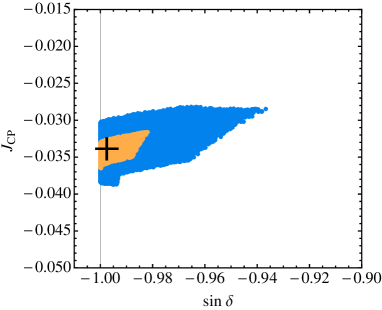
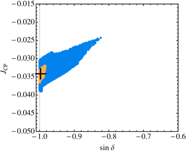
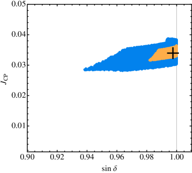
Figure 1: Possible values of $\sin\delta$ and $J_{\text{CP}}$, obtained by using the 1$\sigma$ (light brown areas) and 2$\sigma$ ranges (blue + light brown areas) of allowed values of the mixing angles $\theta_{12}$, $\theta_{23}$ and $\theta_{13}$ for NO spectrum (left panels) and IO spectrum (right panels), and for $\sin\delta<0$ (upper panels) and $\sin\delta>0$ (lower panels). The predictions for the best fit values of $\theta_{12}$, $\theta_{23}$ and $\theta_{13}$, corresponding to $\delta=266.02^{\circ}$ ($\sin\delta<0$) and $\delta=93.98^{\circ}$ ($\sin\delta>0$), are indicated with crosses. See text for further details.

As it follows from Table 1, the angle $\theta_{23}$ is determined using the current neutrino oscillation data with largest uncertainty. We give next the values of the Dirac phase $\delta$ for two values of $\sin^{2}\theta_{23}$ from its $3\sigma$ allowed range, $\sin^{2}\theta_{23}=0.50~{}{\rm and}~{}0.60$, and for the best fit values of $\sin^{2}\theta_{12}$ and $\sin^{2}\theta_{13}$:

$$\sin^{2}\theta_{23}=0.50:~{}~{}\cos\delta=-\,0.123\,,~{}~{}\delta=97.09^{\circ}~{}~{}{\rm or}~{}~{}262.91^{\circ}\,;$$ (3.60)

$$\sin^{2}\theta_{23}=0.60:~{}~{}\cos\delta=-\,0.176\,,~{}~{}\delta=100.12^{\circ}~{}~{}{\rm or}~{}~{}259.88^{\circ}\,.$$ (3.61)

These results show that $|\sin\delta|$, which determines the magnitude of the CP violation effects in neutrino oscillations, exhibits very weak dependence on the value of $\sin^{2}\theta_{23}$: for any value of $\sin^{2}\theta_{23}$ from the interval $0.39\leq\sin^{2}\theta_{23}\leq 0.60$ we get $|\sin\delta|\geq 0.98$.

The predictions of the model for $\delta$ and $J_{\text{CP}}$ will be tested in the experiments searching for CP violation in neutrino oscillations, which will provide information on the value of the Dirac phase $\delta$.

3.5.3 The Majorana CPV Phases

Using the expressions for the angles $\theta^{e}_{12}$ and $\hat{\theta}_{23}$ and for $\cos\phi$ in terms of $\sin\theta_{13}$, $\sin\theta_{12}$ and $\sin\theta_{23}$ and the best fit values of $\sin\theta_{13}$, $\sin\theta_{12}$ and $\sin\theta_{23}$, we can calculate the numerical form of $U_{\rm PMNS}$ from which we can extract the values of the physical CPV Majorana phases. We follow the procedure described in [47]. Obviously, there are two such forms of $U_{\rm PMNS}$ corresponding to the two possible values of $\delta$. In the case of $\delta=266.02^{\circ}$ and $\phi\simeq 102.55^{\circ}$ we find:

$$U_{\rm PMNS}=\left(\begin{array}[]{ccc}0.822\;\text{e}^{-\operatorname{\text{i}}7.47^{\circ}}&0.547\;\text{e}^{\operatorname{\text{i}}16.04^{\circ}}&0.155\;\text{e}^{\operatorname{\text{i}}102.55^{\circ}}\\ 0.436\;\text{e}^{-\operatorname{\text{i}}104.08^{\circ}}&0.658\;\text{e}^{\operatorname{\text{i}}114.67^{\circ}}&0.614\;\text{e}^{\operatorname{\text{i}}102.55^{\circ}}\\ 0.365&-0.517&0.774\\ \end{array}\right)\;\overline{Q}\;.\\$$ (3.62)

Recasting this expression in the form of the standard parametrisation of $U_{\rm PMNS}$ we get:

$$U_{\rm PMNS}=P\;\left(\begin{array}[]{ccc}0.822&0.547&0.155\;\text{e}^{\operatorname{\text{i}}93.98^{\circ}}\\ 0.436\;\text{e}^{\operatorname{\text{i}}169.41^{\circ}}&0.658\;\text{e}^{\operatorname{\text{i}}4.65^{\circ}}&0.614\\ 0.365\;\text{e}^{\operatorname{\text{i}}16.04}&0.517\;\text{e}^{\operatorname{\text{i}}172.53}&0.774\\ \end{array}\right)\;Q_{2}\;\overline{Q}\;,\\$$ (3.63)

where $P={\rm diag}(\text{e}^{\operatorname{\text{i}}(16.04-7.47)^{\circ}},\text{e}^{\operatorname{\text{i}}102.55^{\circ}},1)$, $Q_{2}={\rm diag}(\text{e}^{-\operatorname{\text{i}}16.04^{\circ}},\text{e}^{\operatorname{\text{i}}7.47^{\circ}},1)$ and $\text{e}^{\operatorname{\text{i}}\,93.98^{\circ}}=\text{e}^{-\,\operatorname{\text{i}}(360-93.98)^{\circ}}=\text{e}^{-\operatorname{\text{i}}\,266.02^{\circ}}$.
Similarly, in the case of $\delta=93.98$ and $\phi\simeq 257.45^{\circ}$ we obtain:

$$U_{\rm PMNS}=\left(\begin{array}[]{ccc}0.822\;\text{e}^{\operatorname{\text{i}}7.47^{\circ}}&0.547\;\text{e}^{-\operatorname{\text{i}}16.04^{\circ}}&0.155\;\text{e}^{-\operatorname{\text{i}}102.55^{\circ}}\\ 0.436\;\text{e}^{\operatorname{\text{i}}104.08^{\circ}}&0.658\;\text{e}^{-\operatorname{\text{i}}114.67^{\circ}}&0.614\;\text{e}^{-\operatorname{\text{i}}102.55^{\circ}}\\ 0.365&-0.517&0.774\\ \end{array}\right)\;\overline{Q}\;.\\$$ (3.64)

Extracting again phases in diagonal matrices on the right hand and left hand sides to get the standard parametrisation of $U_{\rm PMNS}$ we find:

$$U_{\rm PMNS}=\tilde{P}\;\left(\begin{array}[]{ccc}0.822&0.547&0.155\;\text{e}^{-\operatorname{\text{i}}93.98^{\circ}}\\ 0.436\;\text{e}^{-\operatorname{\text{i}}169.41^{\circ}}&0.658\;\text{e}^{-\operatorname{\text{i}}4.65^{\circ}}&0.614\\ 0.365\;\text{e}^{-\operatorname{\text{i}}16.04}&0.517\;\text{e}^{-\operatorname{\text{i}}172.53}&0.774\\ \end{array}\right)\;\tilde{Q}_{2}\;\overline{Q}\;,\\$$ (3.65)

where $P={\rm diag}(\text{e}^{\operatorname{\text{i}}(-16.04+7.47)^{\circ}},\text{e}^{-\operatorname{\text{i}}102.55^{\circ}},1)$ and $\tilde{Q}_{2}={\rm diag}(\text{e}^{\operatorname{\text{i}}16.04^{\circ}},\text{e}^{-\operatorname{\text{i}}7.47^{\circ}},1)$. The phases in the matrices $P$ and $\tilde{P}$ can be absorbed by the charged lepton fields and are unphysical. In contrast, the phases in the matrices $Q_{2}$ and $\tilde{Q}_{2}$ contribute to the physical Majorana phases. We can finally write the Majorana phase matrix in the parametrization given in (1.1) ($\phi_{1}=0$):

$$-\frac{\beta_{1}}{2}=\mp 16.04^{\circ}-\beta-\frac{\phi_{3}}{2}\,,~{}~{}\sin\delta=\mp\,0.976\,,$$ (3.66)

$$-\frac{\beta_{2}}{2}=\pm 7.47^{\circ}-\beta-\frac{\phi_{3}-\phi_{2}}{2}\,,~{}~{}\sin\delta=\mp\,0.976\,.$$ (3.67)

In order to calculate the phase $\beta=\gamma-\phi$ we have to find the value of $\gamma$. It follows from Eqs. (3.44) and (3.47) that

$$\cos\gamma=\frac{\sin\theta^{e}_{23}\cos\omega_{e}}{\sqrt{2}\sin\hat{\theta}_{23}}\,,\;\;\;\sin\gamma=\frac{\pm\cos\theta^{e}_{23}-\sin\theta^{e}_{23}\sin\omega_{e}}{\sqrt{2}\sin\hat{\theta}_{23}}\,,$$ (3.68)

$$\cos\phi=\frac{\sin\theta^{e}_{23}\cos\omega_{e}}{\sqrt{2}\cos\hat{\theta}_{23}}\,,\;\;\;\sin\phi=\frac{\mp\cos\theta^{e}_{23}-\sin\theta^{e}_{23}\sin\omega_{e}}{\sqrt{2}\cos\hat{\theta}_{23}}\,,\,$$ (3.69)

where we used the fact that $\psi_{e}=\pm\pi/2$. These equations imply the following relations:

$$\cos\gamma=\cos\phi\,\frac{\cos\hat{\theta}_{23}}{\sin\hat{\theta}_{23}}\,,\hskip 123.76965pt$$ (3.70)

$$\sin\phi\cos\hat{\theta}_{23}+\sin\gamma\sin\hat{\theta}_{23}=-\,\sqrt{2}\sin\theta^{e}_{23}\sin\omega_{e}\,.$$ (3.71)

It is clear from Eq. (3.70) that the value of $\cos\gamma$ can be determined knowing the values of $\cos\phi$ and $\sin\hat{\theta}_{23}$, independently of the values of $\theta^{e}_{23}$ and $\omega_{e}$. This, obviously, allows to find also $|\sin\gamma|$, but not the sign of $\sin\gamma$. In the case of $\sin\theta^{e}_{23}\sin\omega_{e}\ll 1$ of interest, Eq. (3.71) allows to correlate the sign of $\sin\gamma$ with the sign of $\sin\phi$ and thus to determine $\gamma$ for a given $\phi$: we have $\sin\gamma<0$ if $\sin\phi>0$, and $\sin\gamma>0$ for $\sin\phi<0$. Thus, for $\phi=102.5530^{\circ}$ (corresponding to $\delta=266.02^{\circ}$) we find $\gamma=-\,105.4118$ and $\beta=\gamma-\phi=-\,207.9648^{\circ}=-\,(180+27.9648)^{\circ}$, while for $\phi=-\,102.5530^{\circ}$ (corresponding to $\delta=93.98^{\circ}$) we obtain $\gamma=+\,105.4118$ and $\beta=+207.96^{\circ}=+\,(180+27.96)^{\circ}$.

The results thus derived allow us to calculate numerically the Majorana CPV phases. For the best fit values of the neutrino mixing angles we get:

$$\begin{split}&\beta_{1}=(23.84+360+\phi_{3})^{\circ}\;,\;\beta_{2}=(70.88+360-\phi_{2}+\phi_{3})^{\circ}~{}\mbox{for $\phi=-102.55^{\circ}$ ($\delta=93.98^{\circ}$)}\;;~{}~{}~{}\\ \end{split}$$ (3.72)

$$\begin{split}&\beta_{1}=(-23.84-360+\phi_{3})^{\circ}=(-23.84+360+\phi_{3})^{\circ}\;,\\ &\beta_{2}=(-70.88-360-\phi_{2}+\phi_{3})^{\circ}=(-70.88+360-\phi_{2}+\phi_{3})^{\circ}~{}\mbox{for $\phi=102.55^{\circ}$ ($\delta=266.02^{\circ}$)}\;,\\ \end{split}$$ (3.73)

where we have used the fact that $\beta_{1(2)}$ and $\beta_{1(2)}+4\pi$ lead to the same physical results. In the cases of the three types of neutrino mass spectrum allowed by the model, which are characterised, in particular, by specific values of the $\phi_{2}$ and $\phi_{3}$ we find:

• NO A spectrum, i.e., $\phi_{2}=\phi_{3}=0$:

  $$\begin{split}&\beta_{1}=(23.84+360)^{\circ}\;,\;\beta_{2}=(70.88+360)^{\circ}~{}\mbox{for $\phi=-102.55^{\circ}$ ($\delta=93.98^{\circ}$)}\;,\\ &\beta_{1}=(-23.84+360)^{\circ}\;,\;\beta_{2}=(-70.88+360)^{\circ}~{}\mbox{for $\phi=102.55^{\circ}$ ($\delta=266.02^{\circ}$)}\;;\\ \end{split}$$ (3.74)

• NO B spectrum, i.e., $\phi_{2}=0$ and $\phi_{3}=\pi$:

  $$\begin{split}&\beta_{1}=(23.84+540)^{\circ}\;,\;\beta_{2}=(70.88+540)^{\circ}\mbox{for $\phi=-102.55^{\circ}$ ($\delta=93.98^{\circ}$)}\;,\\ &\beta_{1}=(-23.84+540)^{\circ}\;,\;\beta_{2}=(-70.88+540)^{\circ}\mbox{for $\phi=102.55^{\circ}$ ($\delta=266.02^{\circ}$)}\;;\\ \end{split}$$ (3.75)

• IO spectrum, $\phi_{3}=0$ and $\phi_{2}=\pi$:

  $$\begin{split}&\beta_{1}=(23.84+360)^{\circ}\;,\;\beta_{2}=(70.88+180)^{\circ}~{}\mbox{for $\phi=-102.55^{\circ}$ ($\delta=93.98^{\circ}$)}\;,\\ &\beta_{1}=(-23.84+360)^{\circ}\;,\;\beta_{2}=(-70.88+180)^{\circ}~{}\mbox{for $\phi=102.55^{\circ}$ ($\delta=266.02^{\circ}$)}\;,\\ \end{split}$$ (3.76)

where again we have used the fact that $\beta_{1(2)}$ and $\beta_{1(2)}+4\pi$ are physically indistinguishable.

3.5.4 The Neutrinoless Double Beta Decay Effective Majorana Mass

Knowing the values of the neutrino masses and the Majorana and Dirac CPV phases we can derive predictions for the neutrinoless double beta ($(\beta\beta)_{0\nu}$-) decay effective Majorana mass $\left|\langle\!\,m\,\!\rangle\right|$ (see, e.g., [48]). Since $\left|\langle\!\,m\,\!\rangle\right|$ depends only on the cosines of the CPV phases, we get the same result for $\phi=+\,102.55^{\circ}$ ($\delta=266.02^{\circ}$) and $\phi=-\,102.55^{\circ}$ ($\delta=93.98^{\circ}$).

Thus, for $\phi=\pm 102.55^{\circ}$, using the best fit values of the neutrino mixing angles, we obtain:

$$\mbox{$\left|\langle\!\,m\,\!\rangle\right|$}=4.88\times 10^{-3}\,{\rm eV}\,,~{}~{}{\rm NO~{}A~{}spectrum}\,;$$ (3.77)

$$\mbox{$\left|\langle\!\,m\,\!\rangle\right|$}=7.30\times 10^{-3}\,{\rm eV}\,,~{}~{}{\rm NO~{}B~{}spectrum}\,;$$ (3.78)

$$\mbox{$\left|\langle\!\,m\,\!\rangle\right|$}=26.34\times 10^{-3}\,{\rm eV}\,,~{}~{}{\rm IO~{}spectrum}\;.$$ (3.79)

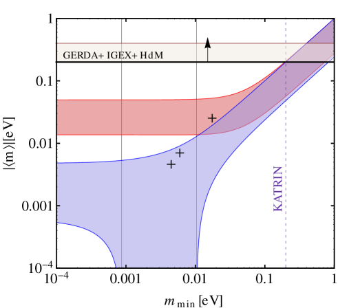
Figure 2: The 3$\sigma$ allowed regions of values of the effective Majorana mass $\left|\langle\!\,m\,\!\rangle\right|$ as functions of the lightest neutrino mass $m_{min}$ for the NO (blue area) and IO (red area) neutrino mass spectra. The regions are obtained by using the experimentally determined values of the neutrino oscillation parameters (including the $1\sigma$ uncertainties) quoted in Table 1. The black crosses correspond to the predictions of the model constructed in the present article, Eqs. (3.77) - (3.79). The horizontal band indicates the upper bound $\mbox{$\left|\langle\!\,m\,\!\rangle\right|$}\sim 0.2-0.4$ eV obtained using the 90 % C.L. limit on the half-life of ⁷⁶Ge reported in [49]. The dotted line represents the prospective upper limit from the $\beta$-decay experiment KATRIN [50].

In Fig. 2 we show the general phenomenologically allowed 3$\sigma$ range of values of $\left|\langle\!\,m\,\!\rangle\right|$ for the NO (blue area) and IO (red area) neutrino mass spectra as a function of the lightest neutrino mass. The values of $\left|\langle\!\,m\,\!\rangle\right|$ quoted above and corresponding to the three types of neutrino mass spectrum (NO A, NO B and IO), predicted by the model constructed in the present article, are indicated with black crosses. The vertical lines in Fig. 2 correspond to $m_{min}=8.6\times 10^{-4}\,{\rm eV}$ and $1.0\times 10^{-2}\,{\rm eV}$; for a given value of $m_{min}$ from the interval determined by these two values, [$8.6\times 10^{-4},1.0\times 10^{-2}$] eV, one can have $\mbox{$\left|\langle\!\,m\,\!\rangle\right|$}=0$ for specific values of the Majorana CPV phases.

3.5.5 Limiting Cases

Finally, there are two interesting limiting forms of the charged lepton Yukawa coupling (mass) matrix ${\rm Y}_{e}$: they correspond to i) $k=0$, i.e., $\eta=0$ or $\pi$, and ii) $d=0$, i.e., $\eta=\pm\pi/2$. In the case of $k=0$, the TBM prediction for $\theta_{12}$ does not depend on $\theta_{23}^{e}$ anymore; if $d=0$, even $\theta_{23}$ itself does not depend on $\theta_{23}^{e}$ anymore. Up to next-to-leading order we find:

$$\begin{split}\text{i) }&\sin^{2}\theta_{12}=\frac{1}{3}+\frac{1}{3}\sin^{2}\theta_{13}\approx\frac{1}{3}\text{ for }k=0,\eta=0,\pi\;,\\ \text{ii) }&\sin^{2}\theta_{23}=\frac{1}{2}-\frac{1}{2}\sin^{2}\theta_{13}\approx\frac{1}{2}\text{ for }d=0,\eta=\pm\pi/2\;,\\ \end{split}$$ (3.80)

where we have written the corrections in terms of $\theta_{13}$. Both cases could be realised by choosing a certain set of messengers. If we remove the messenger pair $\Sigma_{2^{\prime}}^{A}$, $\bar{\Sigma}_{2^{\prime\prime}}^{A}$, our model would correspond to the case i), while if we remove the messenger pair $\Sigma_{1^{\prime\prime}}^{C}$, $\bar{\Sigma}_{1^{\prime}}^{C}$, the model would correspond to the case ii). The model we have constructed, which includes both messenger pairs, gives a somewhat better description of the current data on the neutrino mixing angles. This brief discussion shows how important the messenger sector can be for getting meaningful predictions.

4 Summary and Conclusions

In this work we have analyzed the presence of a generalised CP symmetry, $H_{\text{CP}}$, combined with the non-Abelian discrete group $T^{\prime}$ in the lepton flavour space, i.e. the possibility of the existence of a symmetry group $G_{f}=T^{\prime}\rtimes H_{\text{CP}}$ acting among the three generations of charged leptons and neutrinos. The phenomenological implications of the breaking of such a symmetry group both in the charged lepton and neutrino sectors are thus explored especially in connection with the CP violation appearing in the leptonic mixing matrix, $U_{\text{PMNS}}$.

First of all we have derived in Section 2 all the possible generalised CP transformations for all the representations of the $T^{\prime}$ group i.e. we found all possible outer automorphisms of the group $T^{\prime}$ following the consistency conditions given in [41, 42, 44]. We have chosen as generalised CP symmetry the transformation $u:(T,S)\rightarrow(T^{2},S^{2}T^{2}S\,T)$ which corresponds to a $Z_{2}$ symmetry and it is defined up to an inner automorphism. The transformation $u$ is particularly convenient since, in the basis chosen for the generators $S$ and $T$, for the 1 and 3-dimensional representations it is trivially defined as the identity up to a global unphysical phase $\theta_{r}$ where the index $r$ refers to the representation. More importantly we found that, given this specific generalised CP symmetry combined with $T^{\prime}$, it is possible to fix the vevs of the flavon fields to real values in such a way that no complex phases, and thus no physical CP violation, stem from the vevs themselves.

Moreover, for a list of possible renormalisable operators, namely $\lambda\mathcal{O}=\lambda(A\times B\times C)$ where $\lambda$ is the coupling constant and $A$, $B$, $C$ are fields, we derived the constraints on the phase $\lambda$ under the assumption of invariance under the generalised CP transformation. This list of possible operators can be used to construct a CP-conserving renormalisable superpotential for the flavon sector and therefore can be used in order to show that real vev structures can be achieved.

Motivated by this preliminary study we constructed in Section 3 a supersymmetric flavour model able to describe the observed patterns and mixing for three generations of charged lepton fields and the three light active neutrinos.

We have constructed an effective superpotential with operators up to mass dimension six giving the charged lepton and neutrino Yukawa couplings and the Majorana mass term for the RH neutrinos. Naturally small neutrino masses are generated by the type I see-saw mechanism. At leading order, the mixing in the neutrino sector is described by the tri-bimaximal mixing, which is then perturbed by additional contributions coming from the charged lepton sector. The latter are responsible for the compatibility of the predictions on the mixing angles with the experimental values and, in particular, with the non-zero value of the reactor mixing angle $\theta_{13}$.

Similarly to what was found in [35], we find that both types of neutrino mass spectrum - with normal ordering (NO) and inverted ordering (IO) - are possible within the model and that the NO spectrum can be of two varieties, A and B. They differ by the value of the lightest neutrino mass. Only one spectrum of the IO type is compatible with the model. For each of the three neutrino mass spectra, NO A, NO B and IO, the absolute scale of neutrino masses is predicted with relatively small uncertainty. This allows us to predict the value of the sum of the neutrino masses for the three spectra. The Dirac phase $\delta$ is predicted to be approximately $\delta\cong\pi/2$ or $3\pi/2$. More concretely, for the best fit values of the neutrino mixing angles quoted in Table 1 we get $\delta=93.98^{\circ}$ or $\delta=266.02^{\circ}$. The deviations of $\delta$ from the values $90^{\circ}$ and $270^{\circ}$ are correlated with the deviation of atmospheric neutrino mixing angle $\theta_{23}$ from $\pi/4$. Thus, the CP violating effects in neutrino oscillations are predicted to be nearly maximal (given the values of the neutrino mixing angles) and experimentally observable. The values of the Majorana CPV phases are also predicted by the model. This allows us to predict the neutrinoless double beta decay effective Majorana mass in each of the three cases of neutrino mass spectrum allowed by the model, NO A, NO B and IO. The predictions of the model can be tested in ongoing and future planned i) accelerators experiments searching for CP violation in neutrino oscillations (T2K, NO$\nu$A, etc.), ii) experiments aiming to determine the absolute neutrino mass scale, and iii) experiments searching for neutrinoless double beta decay.

It is important to comment that in this model the physical CP violation emerging in the PMNS mixing matrix stems only from the charged lepton sector. Indeed, in the neutrino sector the Majorana mass matrix and the Dirac Yukawa couplings are real and the CP violation is caused by the complex CP violating phases arising in the charged lepton sector. The presence of the latter is a consequence of the requirement of invariance of the theory under the generalised CP symmetry at the fundamental level and of the complex CGs of the $T^{\prime}$ group.

We also found that the residual group in the charged lepton sector is trivial i.e. $G_{e}=\emptyset$ and since the phases of the flavon vevs are completely independent of the coupling constants of the flavon superpotential, the CP symmetry is broken geometrically (according to the definition of “geometrical CP violation” given in [34]). In the neutrino sector, the residual subgroup is instead a Klein group, $G_{\nu}=K_{4}=Z_{2}\times Z_{2}$ with one $Z_{2}$ coming from the generalised CP symmetry $H_{\text{CP}}$.

Concluding, we have shown that the spontaneous breaking of a symmetry group $G_{f}=T^{\prime}\rtimes H_{\text{CP}}$ in the leptonic sector through a real flavon vev structure is possible and, at the same time, CP violation in the leptonic sector can take place. In this scenario the appearance of the CP violating phases in the PMNS mixing matrix can be traced to two factors: i) the requirement of invariance of the Lagrangian of the theory under $H_{\text{CP}}$ at the fundamental level, and ii) the complex CGs of the $T^{\prime}$ group. The model we have constructed allows for two neutrino mass spectra with normal ordering (NO) and one with inverted ordering (IO). For each of the three spectra the absolute scale of neutrino masses is predicted with relatively small uncertainty. The value of the Dirac CP violation (CPV) phase $\delta$ in the lepton mixing matrix is predicted to be $\delta\cong\pi/2~{}{\rm or}~{}3\pi/2$. Thus, the CP violating effects in neutrino oscillations are predicted to be nearly maximal and experimentally observable. We present also predictions for the sum of the neutrino masses, for the Majorana CPV phases and for the effective Majorana mass in neutrinoless double beta decay. The predictions of the model can be tested in a variety of ongoing and future planned neutrino experiments.

Note added

After the submission of our article to the arXiv, an update of the global fits to the neutrino oscillation data appeared [51]. The results reported in [51] are in agreement with the predictions of our model. More specifically, the authors of [51] find that the best fit value of $\delta$ is $\delta\approx 3\pi/2$, which is one of the two possible values predicted by in our model. Similar results on $\delta$ were obtained in the global analysis of the neutrino oscillation data performed in [52].

Appendix A Technicalities about $\boldsymbol{T^{\prime}}$

The group $T^{\prime}$ is the double covering group of $A_{4}$ and it is defined through the algebraic relations:

$$S^{2}=R\quad R^{2}=T^{3}=(ST)^{3}=E\quad RT=TR\,.$$ (A.1)

The number of the unitary irreducible representations of a discrete group is equal to the number of the conjugacy classes. For $T^{\prime}$ they are seven, which are classified given the elements $T$, $S$, because $R\equiv S^{2}$, we summarize them as

$$\begin{split}&1\,C^{1}:\left\{E\right\}\;,\quad 1^{\prime}\,C^{2}:\left\{S^{2}\right\}\\ &4\,C^{3}:\left\{T,S^{3}TS,ST,TS\right\}\;,\quad 4^{\prime}\,C^{3}:\left\{T^{2},S^{2}TST,S^{2}T^{2}S,S^{3}T^{2}\right\}\\ &4^{\prime\prime}\,C^{6}:\left\{S^{2}T,STS,S^{3}T,S^{2}TS\right\}\;,\quad 4^{\prime\prime\prime}\,C^{6}:\left\{S^{2}T^{2},TST,T^{2}S,ST^{2}\right\}\\ &6\,C^{4}:\left\{S,S^{3},TST^{2},T^{2}ST,S^{2}TST^{2},S^{2}T^{2}ST\right\}\end{split}$$ (A.2)

The representations of $T^{\prime}$ can be expressed as

$$\begin{split}&\mathbf{1}:T=1\;,\;R=1\;,\;S=1\,;\\ &\mathbf{1^{\prime}}:T=\omega\;,\;R=1\;,\;S=1\,;\\ &\mathbf{1^{\prime\prime}}:T=\omega^{2}\;,\;R=1\;,\;S=1\,;\\ &\mathbf{2}:T=\left(\begin{array}[]{cc}\omega^{2}&0\\ 0&\omega\\ \end{array}\right)\;,\;R=\left(\begin{array}[]{cc}-1&0\\ 0&-1\\ \end{array}\right)\;,\;S=\left(\begin{array}[]{cc}-\frac{i}{\sqrt{3}}&-\sqrt{\frac{2}{3}}p\\ \sqrt{\frac{2}{3}}\bar{p}&\frac{i}{\sqrt{3}}\\ \end{array}\right);\\ &\mathbf{2^{\prime}}:T=\left(\begin{array}[]{cc}\omega^{3}&0\\ 0&\omega^{2}\\ \end{array}\right)\;,\;R=\left(\begin{array}[]{cc}-1&0\\ 0&-1\\ \end{array}\right)\;,\;S=\left(\begin{array}[]{cc}-\frac{i}{\sqrt{3}}&-\sqrt{\frac{2}{3}}p\\ \sqrt{\frac{2}{3}}\bar{p}&\frac{i}{\sqrt{3}}\\ \end{array}\right);\\ &\mathbf{2^{\prime\prime}}:T=\left(\begin{array}[]{cc}\omega&0\\ 0&1\\ \end{array}\right)\;,\;R=\left(\begin{array}[]{cc}-1&0\\ 0&-1\\ \end{array}\right)\;,\;S=\left(\begin{array}[]{cc}-\frac{i}{\sqrt{3}}&-\sqrt{\frac{2}{3}}p\\ \sqrt{\frac{2}{3}}\bar{p}&\frac{i}{\sqrt{3}}\\ \end{array}\right);\\ &\mathbf{3}:T=\left(\begin{array}[]{ccc}1&0&0\\ 0&\omega&0\\ 0&0&\omega^{2}\\ \end{array}\right)\;,\;R=\left(\begin{array}[]{ccc}1&0&0\\ 0&1&0\\ 0&0&1\\ \end{array}\right)\;,\;S=\left(\begin{array}[]{ccc}-\frac{1}{3}&\frac{2\omega}{3}&\frac{2\omega^{2}}{3}\\ \frac{2\omega^{2}}{3}&-\frac{1}{3}&\frac{2\omega}{3}\\ \frac{2\omega}{3}&\frac{2\omega^{2}}{3}&-\frac{1}{3}\\ \end{array}\right).\\ \end{split}$$

We use the definition of the representation of $T^{\prime}$ given in [24] in which $\omega$ and $p$ are fixed to be respectively $\omega=\text{e}^{\frac{2\operatorname{\text{i}}\pi}{3}}$ and $p=\text{e}^{\frac{\operatorname{\text{i}}\pi}{12}}$. Finally $T^{\prime}$ has $n=13$ subgroups excluding the whole group:

• Trivial subgroup
  $\mathbb{E}=\left\{E\right\}$;

• $Z_{2}$ subgroup
  $Z^{S^{2}}_{2}=\left\{E,S^{2}\right\}$;

• $Z_{3}$ subgroups
  $Z^{T}_{3}=\left\{E,T,T^{2}\right\}$, $Z^{S^{3}TS}_{3}=\left\{E,S^{3}TS,S^{2}TST\right\}$, $Z^{ST}_{3}=\left\{E,ST,S^{2}T^{2}S\right\}$, $Z^{TS}_{3}=\left\{E,TS,S^{3}T^{2}\right\}$;

• $Z_{4}$ subgroups
  $Z^{S}_{4}=\left\{E,S,S^{2},S^{3}\right\}$, $Z^{TST^{2}}_{4}=\left\{E,TST^{2},S^{2},S^{2}TST^{2}\right\}$, $Z^{T^{2}ST}_{4}=\left\{E,T^{2}ST,S^{2},S^{2}T^{2}ST\right\}$;

• $Z_{6}$ subgroups
  $Z^{S^{2}T}_{6}=\left\{E,S^{2}T,T^{2},S^{2},T,S^{2}T^{2}\right\}$, $Z^{STS}_{6}=\left\{E,STS,S^{2}TST,S^{2},S^{3}TS,TST\right\}$,
  $Z^{S^{3}T}_{6}=\left\{E,S^{3}T,S^{2}T^{2}S,S^{2},ST,T^{2}S\right\}$, $Z^{S^{2}TS}_{6}=\left\{E,S^{2}TS,S^{3}T^{2},S^{2},TS,ST^{2}\right\}$.

A complete table of the CGs coefficients can be found in [35].

Appendix B Messenger Sector

	$SU(2)$	$U(1)_{Y}$	$T^{\prime}$	$U(1)_{R}$	$Z_{8}$	$Z_{4}$	$Z_{4}$	$Z_{3}$	$Z_{3}$	$Z_{2}$
$\Xi_{1}$ , $\bar{\Xi}_{1}$	$\mathbf{2}$ ,$\mathbf{2}$	1,1	$\mathbf{1}$ ,$\mathbf{1}$	0,2	7,1	0,0	0,0	0,0	1,2	0,0
$\Sigma_{1}^{A}$,$\bar{\Sigma}_{1}^{A}$	$\mathbf{2}$ ,$\mathbf{2}$	1,1	$\mathbf{1}$ ,$\mathbf{1}$	1,1	1,7	3,1	3,1	2,1	1,2	1,1
$\Sigma_{1}^{B}$,$\bar{\Sigma}_{1}^{B}$	$\mathbf{1}$ ,$\mathbf{1}$	2,2	$\mathbf{1}$ ,$\mathbf{1}$	1,1	2,6	1,3	1,3	2,1	0,0	1,1
$\Sigma_{1^{\prime}}^{A}$ ,$\bar{\Sigma}_{1^{\prime\prime}}^{A}$	$\mathbf{2}$ ,$\mathbf{2}$	1,1	$\mathbf{1}^{\prime}$,$\mathbf{1}^{\prime\prime}$	1,1	7,1	3,1	3,1	0,0	2,1	0,0
$\Sigma_{1^{\prime}}^{B}$ ,$\bar{\Sigma}_{1^{\prime\prime}}^{B}$	$\mathbf{1}$ ,$\mathbf{1}$	2,2	$\mathbf{1}^{\prime}$,$\mathbf{1}^{\prime\prime}$	1,1	0,0	1,3	1,3	0,0	1,2	0,0
$\Sigma_{1^{\prime\prime}}^{A}$,$\bar{\Sigma}_{1^{\prime}}^{A}$	$\mathbf{2}$ ,$\mathbf{2}$	1,1	$\mathbf{1}^{\prime\prime}$ ,$\mathbf{1}^{\prime}$	1,1	1,7	3,1	3,1	2,1	1,2	1,1
$\Sigma_{1^{\prime\prime}}^{B}$,$\bar{\Sigma}_{1^{\prime}}^{B}$	$\mathbf{2}$ ,$\mathbf{2}$	1,1	$\mathbf{1}^{\prime\prime}$ ,$\mathbf{1}^{\prime}$	1,1	1,7	3,1	1,3	0,0	0,0	0,0
$\Sigma_{1^{\prime\prime}}^{C}$,$\bar{\Sigma}_{1^{\prime}}^{C}$	$\mathbf{2}$ ,$\mathbf{2}$	1,1	$\mathbf{1}^{\prime\prime}$ ,$\mathbf{1}^{\prime}$	1,1	6,2	3,1	0,0	1,2	1,2	0,0
$\Sigma_{2^{\prime}}^{A}$ ,$\bar{\Sigma}_{2^{\prime\prime}}^{A}$	$\mathbf{2}$ ,$\mathbf{2}$	1,1	$\mathbf{2}^{\prime}$,$\mathbf{2}^{\prime\prime}$	1,1	0,0	1,3	0,0	1,2	1,2	0,0
$\Sigma_{2^{\prime\prime}}^{A}$,$\bar{\Sigma}_{2^{\prime}}^{A}$	$\mathbf{2}$ ,$\mathbf{2}$	1,1	$\mathbf{2}^{\prime\prime}$ ,$\mathbf{2}^{\prime}$	1,1	0,0	1,3	0,0	1,2	1,2	0,0
$\Delta_{1}^{A}$,$\bar{\Delta}_{1}^{A}$	$\mathbf{1}$ ,$\mathbf{1}$	0,0	$\mathbf{1}$ ,$\mathbf{1}$	0,2	0,0	2,2	0,0	0,0	0,0	0,0
$\Delta_{1}^{B}$,$\bar{\Delta}_{1}^{B}$	$\mathbf{1}$ ,$\mathbf{1}$	0,0	$\mathbf{1}$ ,$\mathbf{1}$	0,2	0,0	0,0	0,0	2,1	2,1	0,0
$\Delta_{1^{\prime}}^{A}$ ,$\bar{\Delta}_{1^{\prime\prime}}^{A}$	$\mathbf{1}$ ,$\mathbf{1}$	0,0	$\mathbf{1}^{\prime}$,$\mathbf{1}^{\prime\prime}$	0,2	0,0	0,0	0,0	0,0	2,1	0,0
$\Delta_{2^{\prime}}^{A}$ ,$\bar{\Delta}_{2^{\prime\prime}}^{A}$	$\mathbf{1}$ ,$\mathbf{1}$	0,0	$\mathbf{2}^{\prime}$,$\mathbf{2}^{\prime\prime}$	0,2	0,0	0,0	3,1	1,2	1,2	1,1
$\Delta_{3}^{A}$,$\bar{\Delta}_{3}^{A}$	$\mathbf{1}$ ,$\mathbf{1}$	0,0	$\mathbf{3}$ ,$\mathbf{3}$	0,2	4,4	0,0	0,0	0,0	0,0	1,1
$\Delta_{3}^{B}$,$\bar{\Delta}_{3}^{B}$	$\mathbf{1}$ ,$\mathbf{1}$	0,0	$\mathbf{3}$ ,$\mathbf{3}$	0,2	6,2	2,2	0,0	1,2	0,0	1,1
$\Delta_{3}^{C}$,$\bar{\Delta}_{3}^{C}$	$\mathbf{1}$ ,$\mathbf{1}$	0,0	$\mathbf{3}$ ,$\mathbf{3}$	0,2	6,2	1,3	2,2	0,0	1,2	0,0
$\Delta_{3}^{D}$,$\bar{\Delta}_{3}^{D}$	$\mathbf{1}$ ,$\mathbf{1}$	0,0	$\mathbf{3}$ ,$\mathbf{3}$	0,2	5,3	0,0	3,1	0,0	1,2	0,0
$\Delta_{3}^{E}$,$\bar{\Delta}_{3}^{E}$	$\mathbf{1}$ ,$\mathbf{1}$	0,0	$\mathbf{3}$ ,$\mathbf{3}$	0,2	2,6	0,0	2,2	2,1	0,0	0,0

Table 9: List of the messengers fields and their transformation properties.

The effective model we have considered so far contains only non-renormalisable operators allowed by the symmetry group $G_{f}\times Z_{2}\times Z_{3}^{2}\times Z_{4}^{2}\times Z_{8}\times U(1)_{R}$. But in fact using only this symmetry there would be more effective operators allowed which might spoil our model predictions.

Therefore we discuss in in this section we a so-called ultraviolet completion defining a renormalisable theory which gives the effective model described in the previous sections after integrating out the heavy messenger superfields. In this way we can justify why we have chosen only a certain subset of the effective operators allowed by the symmetries. The quantum numbers of the messenger fields are given in Table 9. We label them with $\Sigma$, $\Xi$ and $\Delta$ for the charged lepton, neutrino and flavon sector respectively.

For the charged lepton sector we find the renormalisable superpotential $\mathcal{W}_{e}^{\rm ren}$

$$\begin{split}\mathcal{W}_{e}^{\text{ren}}&=L\,\phi\,\Sigma^{A}_{1^{\prime\prime}}+L\,\phi\,\Sigma^{A}_{1}+\bar{E}_{3}\,H_{d}\,\bar{\Sigma}^{A}_{1^{\prime}}+L\,\hat{\phi}\,\Sigma^{C}_{1^{\prime\prime}}+\zeta\,\bar{\Sigma}_{1^{\prime}}^{C}\,\Sigma_{1^{\prime\prime}}^{A}+H_{d}\,\bar{\Sigma}_{1}^{A}\,\Sigma_{1}^{B}\\ &+\bar{E}\,\psi^{\prime}\,\bar{\Sigma}_{1}^{B}+L\,\psi^{\prime}\,\Sigma_{2^{\prime\prime}}^{A}+\psi^{\prime\prime}\,\bar{\Sigma}_{2^{\prime}}^{A}\,\Sigma_{1}^{A}+L\,\tilde{\phi}\,\Sigma_{1^{\prime}}^{B}+\tilde{\zeta}^{\prime}\,\bar{\Sigma}_{1^{\prime}}^{B}\,\Sigma_{1^{\prime}}^{B}\\ &+H_{d}\,\bar{\Sigma}_{1^{\prime\prime}}^{B}\,\Sigma_{1^{\prime}}^{C}+\bar{E}\,\tilde{\psi}^{\prime\prime}\,\bar{\Sigma}_{1^{\prime\prime}}^{C}+L\,\psi^{\prime}\,\Sigma_{2^{\prime}}^{A}+\psi^{\prime\prime}\,\bar{\Sigma}_{2^{\prime\prime}}^{A}\,\Sigma_{1^{\prime\prime}}^{A}\;,\end{split}$$ (B.1)

which through the diagrams of Fig. 3 generates at low energy the non-renormalisable superpotential $\mathcal{W}_{{\rm Y}_{e}}$ of Eq. (3.12).

For the neutrino and the flavon sector we obtained similarly to the previous case

$$\mathcal{W}_{\nu}^{\text{ren}} =N^{2}\xi+N^{2}\rho+N^{2}\tilde{\rho}+LN\Xi_{1}+H_{u}\bar{\Xi}_{1}\rho+H_{u}\bar{\Xi}_{1}\tilde{\rho}\;,$$ (B.2)

$$\begin{split}\mathcal{W}_{\text{flavon}}^{\text{ren}}&=D_{\phi}\,\phi\,\Delta_{3}^{B}+\varepsilon_{3}\,\phi\,\bar{\Delta}_{3}^{B}+D_{\phi}\,\zeta^{\prime\prime}\,\Delta_{3}^{B}+\tilde{D}_{\phi}\,\tilde{\phi}\,\Delta_{3}^{C}+\varepsilon_{1}\,\tilde{\phi}\,\bar{\Delta}_{3}^{C}+\tilde{D}_{\phi}\,\tilde{\zeta}^{\prime}\,\Delta_{3}^{C}\\ &+\hat{D}_{\phi}\,\hat{\phi}\,\Delta_{3}^{D}+\varepsilon_{4}\,\hat{\phi}\,\bar{\Delta}_{3}^{D}+\hat{D}_{\phi}\,\tilde{\zeta}^{\prime\prime}\,\Delta_{3}^{E}+\varepsilon_{5}\,\tilde{\phi}\,\bar{\Delta}_{3}^{E}+\tilde{S}_{\zeta}\,\tilde{\zeta}^{\prime\prime}\,\Delta_{1^{\prime}}^{A}+\tilde{\zeta}^{\prime\prime}\,\tilde{\zeta}^{\prime\prime}\,\bar{\Delta}_{1^{\prime\prime}}^{A}\\ &+S_{\varepsilon_{4}}\,\varepsilon_{4}\,\Delta_{1}^{B}+\varepsilon_{4}\,\varepsilon_{4}\,\bar{\Delta}_{1}^{B}+\varepsilon_{1}\,\varepsilon_{1}\,\bar{\Delta}_{1}^{A}+S_{\varepsilon_{1}}\,\Delta_{1}^{A}\,\Delta_{1}^{A}\;.\end{split}$$ (B.3)

The corresponding diagrams that generate the effective operators in the neutrino and flavon sector in our model are given in Figs. 4 and 5.

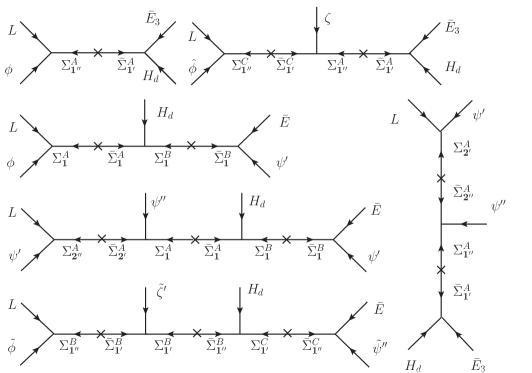
Figure 3: The supergraphs before integrating out the messengers for the charged lepton sector.

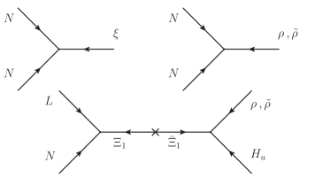
Figure 4: The supergraphs before integrating out the messengers for the neutrino sector.

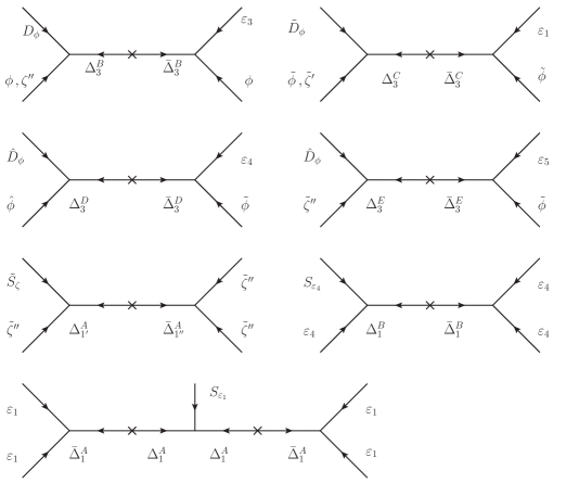
Figure 5: The supergraphs before integrating out the messengers for the flavon sector. We have omitted for simplicity the supergraphs of the higher order corrections in the flavon superpotential.

References

- [1] K. Nakamura and S. T. Petcov, in J. Beringer et al. (Particle Data Group), Phys. Rev. D 86 (2012) 010001.
- [2] S.M. Bilenky, J. Hosek and S.T. Petcov, Phys. Lett. B 94 (1980) 495.
- [3] E. Molinaro and S. T. Petcov, Eur. Phys. J. C 61 (2009) 93.
- [4] A. Ibarra, E. Molinaro and S. T. Petcov, Phys. Rev. D 84 (2011) 013005.
- [5] L. Wolfenstein, Phys. Lett. B 107 (1981) 77; S.M. Bilenky, N.P. Nedelcheva and S.T. Petcov, Nucl. Phys. B 247 (1984) 61; B. Kayser, Phys. Rev. D 30 (1984) 1023.
- [6] G. L. Fogli, E. Lisi, A. Marrone, D. Montanino, A. Palazzo and A. M. Rotunno, Phys. Rev. D 86 (2012) 013012.
- [7] M. C. Gonzalez-Garcia, M. Maltoni, J. Salvado and T. Schwetz, JHEP 1212 (2012) 123.
- [8] C. Giunti and M. Tanimoto, Phys. Rev. D 66 (2002) 053013, Phys. Rev. D 66 (2002) 113006.
- [9] P.H. Frampton, S.T. Petcov and W. Rodejohann, Nucl. Phys. B 687 (2004) 31.
- [10] S.T. Petcov and W. Rodejohann, Phys. Rev. D71 (2005) 073002.
- [11] A. Romanino, Phys. Rev. D 70 (2004) 013003.
- [12] K.A. Hochmuth, S.T. Petcov and W. Rodejohann, Phys. Lett B 654 (2007) 177.
- [13] D. Marzocca, S. T. Petcov, A. Romanino, M. Spinrath, JHEP 11 (2011) 009.
- [14] D. Marzocca, S. T. Petcov, A. Romanino and M. C. Sevilla, JHEP 1305 (2013) 073.
- [15] G. Altarelli, F. Feruglio and I. Masina, Nucl. Phys. B 689 (2004) 157; S. F. King, JHEP 0508 (2005) 105; I. Masina, Phys. Lett. B 633 (2006) 134; S. Antusch and S. F. King, Phys. Lett. B 631 (2005) 42; S. Dev, S. Gupta and R. R. Gautam, Phys. Lett. B 704 (2011) 527; S. Antusch and V. Maurer, Phys. Rev. D 84 (2011) 117301; A. Meroni, S.T. Petcov and M. Spinrath, Phys. Rev. D 86 (2012) 113003; C. Duarah, A. Das and N. N. Singh, [arXiv:1210.8265].
- [16] W. Chao and Y. -j. Zheng, JHEP 1302 (2013) 044; D. Meloni, JHEP 1202 (2012) 090; S. Antusch, C. Gross, V. Maurer and C. Sluka, Nucl. Phys. B 866 (2013) 255; G. Altarelli, F. Feruglio, L. Merlo and E. Stamou, JHEP 1208 (2012) 021; G. Altarelli, F. Feruglio and L. Merlo, [arXiv:1205.5133]; F. Bazzocchi and L. Merlo, [arXiv:1205.5135]; S. Gollu, K. N. Deepthi and R. Mohanta, [arXiv:1303.3393].
- [17] C. H. Albright, A. Dueck and W. Rodejohann, Eur. Phys. J. C 70 (2010) 1099.
- [18] P. F. Harrison, D. H. Perkins and W. G. Scott, Phys. Lett. B 530 (2002) 167; Phys. Lett. B 535 (2002) 163; Z. Z. Xing, Phys. Lett. B 533 (2002) 85; X. G. He and A. Zee, Phys. Lett. B 560 (2003) 87; see also L. Wolfenstein, Phys. Rev. D 18 (1978) 958.
- [19] S.T. Petcov, Phys. Lett. B 110 (1982) 245.
- [20] F. Vissani, [arXiv:hep-ph/9708483]; V. D. Barger, S. Pakvasa, T. J. Weiler and K. Whisnant, Phys. Lett. B 437 (1998) 107; A. J. Baltz, A. S. Goldhaber and M. Goldhaber, Phys. Rev. Lett. 81 (1998) 5730.
- [21] S. F. King and C. Luhn, Rept. Prog. Phys. 76 (2013) 056201.
- [22] G. Altarelli and F. Feruglio, Rev. Mod. Phys. 82 (2010) 2701.
- [23] H. Ishimori et al., Prog. Theor. Phys. Suppl. 183 (2010) 1.
- [24] P. H. Frampton and T. W. Kephart, Int. J. Mod. Phys. A 10 (1995) 4689; F. Feruglio, C. Hagedorn, Y. Lin and L. Merlo, Nucl. Phys. B 775 (2007) 120 [Erratum-ibid. 836 (2010) 127]; G. J. Ding, Phys. Rev. D 78 (2008) 036011; P. H. Frampton, T. W. Kephart and S. Matsuzaki, Phys. Rev. D 78 (2008) 073004; D. A. Eby, P. H. Frampton and S. Matsuzaki, Phys. Lett. B 671 (2009) 386; P. H. Frampton and S. Matsuzaki, Phys. Lett. B 679 (2009) 347.
- [25] M.-C. Chen and K. T. Mahanthappa, Phys. Lett. B 652 (2007) 34.
- [26] M.-C. Chen and K. T. Mahanthappa, Phys. Lett. B 681 (2009) 444.
- [27] F. P. An et al. [DAYA-BAY Collaboration], Phys. Rev. Lett. 108 (2012) 171803.
- [28] J. K. Ahn et al. [RENO Collaboration], Phys. Rev. Lett. 108 (2012) 191802.
- [29] K. Abe et al. [T2K Collaboration], Phys. Rev. Lett. 107 (2011) 041801.
- [30] Y. Abe et al. [DOUBLE-CHOOZ Collaboration], Phys. Rev. Lett. 108 (2012) 131801; Y. Abe et al. [DOUBLE-CHOOZ Collaboration], Phys. Rev. D 86 (2012) 052008.
- [31] P. Adamson et al. [MINOS Collaboration], Phys. Rev. Lett. 107 (2011) 181802.
- [32] P. Minkowski, Phys. Lett. B 67 (1977) 421; M. Gell-Mann, P. Ramond and R. Slansky in Sanibel Talk, CALT-68-709, Feb 1979, and in Supergravity (North Holland, Amsterdam 1979); T. Yanagida in Proc. of the Workshop on Unified Theory and Baryon Number of the Universe, KEK, Japan, 1979; S.L.Glashow, Cargese Lectures (1979); R. N. Mohapatra and G. Senjanovic, Phys. Rev. Lett. 44 (1980) 912.
- [33] J.-Q. Chen and P.-D. Fan, J. Math. Phys. 39 (1998) 5519.
- [34] G. C. Branco, J. M. Gerard and W. Grimus, Phys. Lett. B 136 (1984) 383.
- [35] A. Meroni, S. T. Petcov and M. Spinrath, Phys. Rev. D 86 (2012) 113003.
- [36] M. -C. Chen, J. Huang, K. T. Mahanthappa and A. M. Wijangco, arXiv:1307.7711.
- [37] S. Antusch, S. F. King, C. Luhn and M. Spinrath, Nucl. Phys. B 850 (2011) 477.
- [38] S. Antusch, S. F. King and M. Spinrath, Phys. Rev. D 87 (2013) 096018; S. F. King, JHEP 1307 (2013) 137 and arXiv:1305.4846; S. Antusch, C. Gross, V. Maurer and C. Sluka, arXiv:1305.6612 and arXiv:1306.3984.
- [39] S. Antusch and V. Maurer, Phys. Rev. D 84 (2011) 117301.
- [40] S. Antusch and M. Spinrath, Phys. Rev. D 79 (2009) 095004; M. Spinrath, arXiv:1009.2511; S. Antusch, S. F. King and M. Spinrath, arXiv:1311.0877.
- [41] M. Holthausen, M. Lindner and M. A. Schmidt, JHEP 1304 (2013) 122.
- [42] F. Feruglio, C. Hagedorn and R. Ziegler, JHEP 1307 (2013) 027.
- [43] A. Aranda, C. D. Carone and R. F. Lebed, Phys. Rev. D 62 (2000) 016009.
- [44] G.J. Ding, S. F. King and A. J. Stuart, arXiv:1307.4212.
- [45] W. Grimus and P. O. Ludl, J. Phys. A 45 (2012) 233001.
- [46] P.I. Krastev and S. T. Petcov, Phys. Lett. B 205 (1988) 84.
- [47] A. Meroni, E. Molinaro and S.T. Petcov, Phys. Lett. B 710 (2012) 435;
- [48] S. M. Bilenky and S. T. Petcov, Rev. Mod. Phys. 59 (1987) 671;W. Rodejohann, Int. J. Mod. Phys. E20 (2011) 1833.
- [49] M. Agostini et al., arXiv:1307.4720.
- [50] K. Eitel et al., Nucl. Phys. Proc. Suppl. 143 (2005) 197.
- [51] F. Capozzi, G. L. Fogli, E. Lisi, A. Marrone, D. Montanino and A. Palazzo, arXiv:1312.2878 [hep-ph].
- [52] M. C. Gonzales-Garcia et al., talk given at the International Workshop TAUP 2013, September 9-13, 2013, Asilomar, USA.