An Algorithmic Theory of Dependent Regularizers
Part 1: Submodular Structure

Abstract

We present an exploration of the rich theoretical connections between several classes of regularized models, network flows, and recent results in submodular function theory. This work unifies key aspects of these problems under a common theory, leading to novel methods for working with several important models of interest in statistics, machine learning and computer vision.

In Part 1, we review the concepts of network flows and submodular function optimization theory foundational to our results. We then examine the connections between network flows and the minimum-norm algorithm from submodular optimization, extending and improving several current results. This leads to a concise representation of the structure of a large class of pairwise regularized models important in machine learning, statistics and computer vision.

In Part 2, we describe the full regularization path of a class of penalized regression problems with dependent variables that includes the graph-guided LASSO and total variation constrained models. This description also motivates a practical algorithm. This allows us to efficiently find the regularization path of the discretized version of TV penalized models. Ultimately, our new algorithms scale up to high-dimensional problems with millions of variables.

1 Introduction

High-dimensional data is a central focus of modern research in statistics and machine learning. Recent technological advances in a variety of scientific fields for gathering and generating data, matched by rapidly increasing computing power for analysis, has attracted significant research into the statistical questions surrounding structured data. Numerous models and computational techniques have emerged recently to work with these data types.

Our primary contribution is a theoretical framework enabling the efficient optimization of models that work with high-dimensional models in which the predictors are believed to be dependent, correlated, or sparse. In particular, we propose a new approach for estimation of certain types of dependent predictors, in which the model incorporates a prior belief that many of the predictors take similar or identical values. This has been a hot topic of research in recent years, with applications in genomics, image analysis, graphical models, and several other areas. However, efficient estimation involving structured and dependent predictors has proven to be quite challenging. Our main contribution, which includes a number of related theoretical results, is a theoretical framework and algorithmic approach that unlocks a large and particularly thorny class of these models.

After laying out the context for our research in the next section, we outline our main results as well as the needed background in section 3. Our contributions build on recent results in optimization theory and combinatorial optimization, which we describe in detail. In 4, we present a clear theoretical connection between submodular optimization theory, network flows, and the proximal operator in regularized models such as the graph-guided LASSO. Then, in 5, we extend the underlying submodular optimization theory to allow a weighted version of the underlying submodular problem. In the context of regularized regression, this allows the use of additional unary terms in the regularizer.

2 Overview of Statistical Models and Regularization

To begin, consider a simple regression model, in which we have $N$ observations ${{\mathbf{y}}}=(\boldsymbol{\mathbf{y}}_{1},{{\mathbf{y}}}_{2},...,\boldsymbol{\mathbf{y}}_{N})$ and $n$ predictors $\boldsymbol{\mathbf{u}}=(u_{1},u_{2},...,u_{n})$, with

$${{\mathbf{y}}}_{i}={{\mathbf{A}}}\boldsymbol{\mathbf{u}}+{{\boldsymbol{\varepsilon}}}_{i},\qquad i=1,2,...,N$$ (1)

where ${{\boldsymbol{\varepsilon}}}_{1},{{\boldsymbol{\varepsilon}}}_{2},...,{{\boldsymbol{\varepsilon}}}_{N}$ are independent random noise vectors with $\,\mathrm{E}\,{{\boldsymbol{\varepsilon}}}_{i}=\boldsymbol{\mathbf{0}}$; typically, these are assumed to be i.i.d. Gaussian. In many high dimensional contexts, the estimation of ${\hat{{\mathbf{u}}}}$ may be problematic using classical methods. For example, $n$ may be much larger than $N$, making the problem ill-posed as many possible values of $\boldsymbol{\mathbf{u}}$ map to the same response. ($n$ and $N$ are used here instead of the more common $p$ and $n$ to be consistent with the optimization literature we connect this problem to.) Additionally, many predictors of interest may have a negligible or nearly identical affect on ${{\mathbf{y}}}$; eliminating or grouping these predictors is then desirable. To handle this, a number of sophisticated approaches have been proposed to incorporate variable selection or aggregation into the statistical estimation problem.

One common and well-studied approach is to add a penalty term, or regularizer, to the log-likelihood that enforces some prior belief about the structure of $\boldsymbol{\mathbf{u}}$ (Bickel et al., 2006; Hastie et al., 2009). In this setup, estimating the predictor $\boldsymbol{\mathbf{u}}$ involves finding the minimizer of a log-likelihood term or loss function ${\mathcal{L}}$ plus a regularization term $\Phi$:

$${\hat{{\mathbf{u}}}}=\operatorname*{\;argmin\;}_{\boldsymbol{\mathbf{u}}\in\mathbb{R}^{n}}{\mathcal{L}}(\boldsymbol{\mathbf{u}},{{\mathbf{y}}})+\lambda\Phi(\boldsymbol{\mathbf{u}}),$$ (2)

where $\lambda$ controls the strength of the regularization $\lambda\Phi(\boldsymbol{\mathbf{u}})$.

Many well studied and frequently used models fall into this context. For example, if ${\mathcal{L}}$ is the log-likelihood from a multivariate Gaussian distribution, one of the oldest regularization techniques is the $L_{2}$-norm, which gives us the classic technique of ridge regression (Hoerl and Kennard, 1970), where

$${\hat{{\mathbf{u}}}}_{\text{ridge}}=\operatorname*{\;argmin\;}_{\boldsymbol{\mathbf{u}}\in\mathbb{R}^{n}}\left\lVert{{\mathbf{y}}}-{{\mathbf{A}}}\boldsymbol{\mathbf{u}}\right\rVert_{\!\text{\hskip 0.35002pt}2}^{\!\text{\hskip 0.35002pt}2}+\lambda\left\lVert\boldsymbol{\mathbf{u}}\right\rVert_{\!\text{\hskip 0.35002pt}2}^{\!\text{\hskip 0.35002pt}2}.$$ (3)

In this example, the regularization term is typically used as an effective way of dealing with an ill-conditioned inverse problem in the least squares context or as a simple way of preventing $\boldsymbol{\mathbf{u}}$ from over-fitting the model (Bishop, 2006).

In the Bayesian context, (2) often corresponds directly to finding the maximum a posteriori estimate in the classic likelihood-prior formulation, i.e.

$$p(\boldsymbol{\mathbf{u}}\hskip 1.00006pt\mid\hskip 1.00006pt\boldsymbol{\mathbf{y}}) \propto p(\boldsymbol{\mathbf{y}}\hskip 1.00006pt\mid\hskip 1.00006pt\boldsymbol{\mathbf{u}})p(\boldsymbol{\mathbf{u}}\;;\;\lambda,\theta)$$ (4)

$$\propto e^{-{\mathcal{L}}(\boldsymbol{\mathbf{u}},{{\mathbf{y}}})}\times e^{-\lambda\Phi_{\theta}(\boldsymbol{\mathbf{u}})}.$$ (5)

where $\lambda$ and $\theta$ are hyperparameters controlling the behavior of the prior distribution. In this formulation, the prior captures the belief encoded by the regularization term. For example, the ridge regression problem of (3) corresponds to using a standard multivariate Gaussian likelihood but assumes a $0$-mean spherical Gaussian prior distribution over $\boldsymbol{\mathbf{u}}$.

More recently, the Least Absolute Shrinkage and Selection Operator (LASSO), is used frequently to promote sparsity in the resulting estimator (Tibshirani, 1996; Hastie et al., 2005, 2009). This approach uses the $L_{1}$-norm as the regularization term, i.e.

$${\hat{{\mathbf{u}}}}_{\text{lasso}}=\operatorname*{\;argmin\;}_{\boldsymbol{\mathbf{u}}\in\mathbb{R}^{n}}\left\lVert{{\mathbf{y}}}-{{\mathbf{A}}}\boldsymbol{\mathbf{u}}\right\rVert_{\!\text{\hskip 0.35002pt}2}^{\!\text{\hskip 0.35002pt}2}+\lambda\left\lVert\boldsymbol{\mathbf{u}}\right\rVert_{\!\text{\hskip 0.35002pt}1}$$ (6)

The LASSO problem has been analyzed in detail as a method for simultaneous estimation and variable selection, as the $L_{1}$ penalty tends to set many of the predictors to $0$. The consistency and theoretical properties of this model, for both estimation and variable selection, are well studied (Meinshausen and Yu, 2009; Bunea et al., 2007, 2006; Van De Geer, 2008; van de Geer, 2007; Bickel et al., 2006). Many variants of this problem have also been proposed and analyzed. These include the elastic net, in which $\Phi(\boldsymbol{\mathbf{u}})=\alpha\left\lVert\boldsymbol{\mathbf{u}}\right\rVert_{\!\text{\hskip 0.35002pt}1}+(1-\alpha)\left\lVert\boldsymbol{\mathbf{u}}\right\rVert_{\!\text{\hskip 0.35002pt}2}^{\!\text{\hskip 0.35002pt}2}$, with $\alpha\in{\left[0,1\right]}$; this generalizes both ridge regression and LASSO (Zou and Hastie, 2005). Data-adaptive versions of these estimators are analyzed in (Zou, 2006; Zou and Hastie, 2005; Zou and Zhang, 2009). In addition, there are many efficient algorithms to quickly solve these problems, which is one of the reasons they are used frequently in practice (Friedman et al., 2008a, 2010, 2007; Efron et al., 2004; Beck and Teboulle, 2009).

2.1 Graph Structured Dependencies

While there are other possible regularization strategies on individual parameters, of most interest to us is the incorporation of correlation structures and dependencies among the predictors into the prior distribution or regularization term. In many cases, this translates into penalizing the differences of predictors. This has recently been attracting significant algorithmic and theoretical interest as a way to effectively handle dependency structures in the data.

In our particular context, we are interested in the MAP estimate of models with Markov Random Field prior. The resulting log-linear models consist of a collection of unary and pairwise terms that capture the dependency structure of the problem. In particular, the priors we are interested in enforce similarity between neighboring variables, where “neighbor” is defined according to the graph structure of the MRF prior. The type of dependency we are looking at is determined by the

The simplest form of model dependency in the parameters is captured by the Fused LASSO problem (Tibshirani et al., 2005), which penalizes pairwise differences between terms in an ordered problem to be

$$\boldsymbol{\mathbf{u}}^{*}_{\text{fused}}=\operatorname*{\;argmin\;}_{\boldsymbol{\mathbf{u}}\in\mathbb{R}^{n}}=\left\lVert{{\mathbf{A}}}\boldsymbol{\mathbf{u}}-{{\mathbf{y}}}\right\rVert_{\!\text{\hskip 0.35002pt}2}^{\!\text{\hskip 0.35002pt}2}+\lambda\left[w_{1}\left\lVert\boldsymbol{\mathbf{u}}\right\rVert_{\!\text{\hskip 0.35002pt}1}+w_{2}\sum_{i=1}^{n-1}{\left\lvert u_{i+1}-u_{i}\right\rvert}\right],$$ (7)

where $w_{1},w_{2}\geq 0$ control the balance between the $L_{1}$-norm controlling variable sparsity and the sum of ordered differences that effectively penalizes changepoints. This problem has gained some recent attention in the statistics community in the context of non-parametric regression (Dümbgen and Kovac, 2009; Cho and Fryzlewicz, 2011; Davies and Meise, 2008), group sparsity (Tibshirani et al., 2005; Bleakley and Vert, 2011), and change-point detection (Bleakley and Vert, 2011). From the optimization perspective, several algorithms to find the solution to this problem have been proposed; we refer the reader to Liu et al. (2010); Ye and Xie (2011); Bach et al. (2012) or Friedman et al. (2007) for discussions of this particular problem.

The generalized problem, in which the pairwise terms are not required to be ordered, is of significant practical interest in both the statistics and machine learning communities. Here, the pairwise interactions are controlled with an arbitrary graph of weighted difference penalties:

$$\boldsymbol{\mathbf{u}}^{*}_{\text{graph}}=\operatorname*{\;argmin\;}_{\boldsymbol{\mathbf{u}}\in\mathbb{R}^{n}}=\left\lVert{{\mathbf{y}}}-{{\mathbf{A}}}\boldsymbol{\mathbf{u}}\right\rVert_{\!\text{\hskip 0.35002pt}2}^{\!\text{\hskip 0.35002pt}2}+\lambda\left[w_{1}\left\lVert\boldsymbol{\mathbf{u}}\right\rVert_{\!\text{\hskip 0.35002pt}1}+\sum_{1\leq i<j\leq n}w_{ij}{\left\lvert u_{i}-u_{j}\right\rvert}\right],$$ (8)

where $w_{1}\geq 0$ controls the sparsity of the individual predictors, and $w_{ij}\geq 0$ penalizes differences, typically between predictors known to be correlated. This problem has become known as the graph guided LASSO Yu (2013).

This model – often with $w_{1}=0$ – arises in the context of “roughness” penalized regression in which differences between neighboring regions are penalized (Belkin et al., 2004). Besag, Green, Higdon, and Mengersen (1995) examined pairwise interactions on Markov random fields, which describe a prior distribution on the edges of an undirected graph; the proposed models were then solved with MCMC methods. Similar problems also arise in the estimation of sparse covariance matrices as outlined by Friedman, Hastie, and Tibshirani (2008b); there, structure learning is the goal and the pairwise interaction terms are not formed explicitly.

Similarly, Kovac and Smith (2011) analyzes this model as an approach to nonparametric regression on a graph, although with the simpler case of ${{\mathbf{A}}}={{\mathbf{I}}}$. He proposes an efficient active-region based procedure to solve the resulting optimization problem. In the genomics community, a version of (8) has been proposed as the Graph-Guided Fused LASSO problem by Kim, Sohn, and Xing (2009). There, the pairwise interactions were estimated from the correlation structure in the quantitative traits. Their model is essentially identical to this one, though with $w_{1}=0$. There, the authors used a general quadratic solver to tackle the problem and showed good statistical performance in detecting genetic markers. The use of recent results in optimization, in particular proximal operator methods (Nesterov, 2007), have been proposed as a way of optimizing this model Chen, Kim, Lin, Carbonell, and Xing (2010, 2012); Bach, Jenatton, Mairal, and Obozinski (2012). The resulting algorithms, discovered independently, are similar to the ones we propose, although we improve upon them in several ways.

Some recent approaches focus on approximate methods with provable bounds on the solution. Nesterov proposed a smooth approximation approach which can be applied to the graph-guided LASSO in Nesterov (2007). More recently, Yu (2013) proposed a non-smooth approximation method that decomposes the summation in (8).

A very similar model to (8) is proposed in Sharma, Bondell, and Zhang (2013); there, however, the authors include an additional regularization term penalizing ${\left\lvert u_{i}+u_{j}\right\rvert}$. In addition, they give several adaptive schemes for choosing the weights in a way that depends on the correlation structures of the design matrix. This work is noteworthy in that the authors give a detailed analysis of the asymptotic convergence and estimation rate of the model when the regularization weights are chosen adaptively. Their optimization method, however, involves a simple quadratic programming setup, which can severely limit the size of the problems for which their estimator can be used.

In the context of regularized regression with pairwise dependencies, our contribution is a theoretical treatment and several algorithms for a class of models that generalizes (8). Namely, we allow the ${\left\lvert u_{i}\right\rvert}$ penalty in the $L_{1}$ norm to be replaced with an arbitrary convex piecewise linear function $\xi_{i}(u_{i})$. In particular, we examine the estimator

$$\boldsymbol{\mathbf{u}}^{*}_{\star}=\operatorname*{\;argmin\;}_{\boldsymbol{\mathbf{u}}\in\mathbb{R}^{n}}{\mathcal{L}}{\left(\boldsymbol{\mathbf{u}},\boldsymbol{\mathbf{y}}\right)}+\lambda\left[\sum_{i}\xi_{i}(u_{i})+\sum_{1\leq i<j\leq n}w_{ij}{\left\lvert u_{i}-u_{j}\right\rvert}\right],$$ (9)

which generalizes many of the above models. While our primary result is a representation of the theoretical structures underlying this optimization problem, our work motivates efficient and novel algorithms for working with these types of structure. The theory we develop leads to proofs of the correctness of our algorithms. In addition, we are able to present an algorithmic description that gives the entire regularization path for one version of this problem.

2.2 Total Variation Models

Total variation models are effectively an extension of the above pairwise regularization schemes to the estimation of continuous functions. In this context, we wish to estimate a function $u$ in which the total variation of $u$ – the integral of the norm of the gradient – is controlled. This model is used heavily in developing statistical models of images (Chambolle et al., 2010) and the estimation of density functions (Bardsley and Luttman, 2009), but arises in other contexts as well.

When dealing with total variation models, we work theoretically with general $L_{2}$-measurable functions with bounded variation. Our response becomes a function $f$, and our predictor becomes a function $u$. However, in practice, we discretize the problem by working with the functions $f$ and $u$ only on a discrete lattice of points, as is common in these problems.

Let $\Omega\subset\mathbb{R}^{d}$ be a compact region, and let $u$ be an $L_{1}$-integrable continuously differentiable function defined on $\Omega$. In this context, the total variation of $u$ is given by

$$\operatorname{TV}(u)=\int_{\Omega}\left\lVert\nabla\,u\right\rVert_{\!\text{\hskip 0.35002pt}2}\mathrm{d}\mu=\int_{\Omega}\left\lVert(\nabla\,u)({{\mathbf{x}}})\right\rVert_{\!\text{\hskip 0.35002pt}2}\mathrm{d}{{\mathbf{x}}}.$$ (10)

More general definitions exist when $u$ is not continuously differentiable Ambrosio and Di Marino (2012); Giusti (1984); for simplicity, we assume this condition. Let ${\mathcal{F}}(\Omega)$ represent the space of $L_{1}$-integrable continuously differentiable functions of bounded variation. Here, bounded variation can be taken as the condition

$$\operatorname{TV}(u)<+\infty.$$ (11)

Again, much more general definitions exist, but this suffices for our purposes.

Formally, then, the total variation problem seeks to find an estimation function $u^{*}$ that to a function $f\,\,\mathbf{:}\,\,\mathbb{R}^{d}\supset\Omega\mapsto\mathbb{R}$ under a constraint or penalty on the total norm of the gradient of $u$.

$$u^{*} =\operatorname*{\;argmin\;}_{u\in{\mathcal{F}}(\Omega)}\left\lVert u-f\right\rVert_{\!\text{\hskip 0.35002pt}2}^{\!\text{\hskip 0.35002pt}2}+\lambda\operatorname{TV}(u)$$ (12)

$$=\operatorname*{\;argmin\;}_{u\in{\mathcal{F}}(\Omega)}\int_{\Omega}(u({{\mathbf{x}}})-f({{\mathbf{x}}}))^{2}\mathrm{d}{{\mathbf{x}}}+\lambda\operatorname{TV}(u)$$ (13)

This model – often called the Rudin-Osher-Fatimi (ROF) model after the authors – was originally proposed in Rudin et al. (1992) as a way of removing noise from images corrupted by Gaussian white noise; however, it has gained significant attention in a variety of other areas.

In the image analysis community, it has been used often as a model for noise removal, with the solution of (10) being the estimation of the noise-free image. In addition, the value of the total variation term in the optimal solution is often used as a method of edge detection, as the locations of the non-zero gradients tend to track regions of significant change in the image.

Beyond image analysis, a number of recent models have used total variation regularization as a general way to enforce similar regions of the solution to have a common value. In this way, it is a generalization of the behavior of the Fused LASSO in one dimension; it tends to set regions of the image to constant values. As such, it is used in MRI reconstruction, electron tomography (Goris et al., 2012; Gao et al., 2010), MRI modeling (Michel et al., 2011; Keeling et al., 2012), CT reconstruction (Tian et al., 2011), and general ill-posed problems (Bardsley and Luttman, 2009).

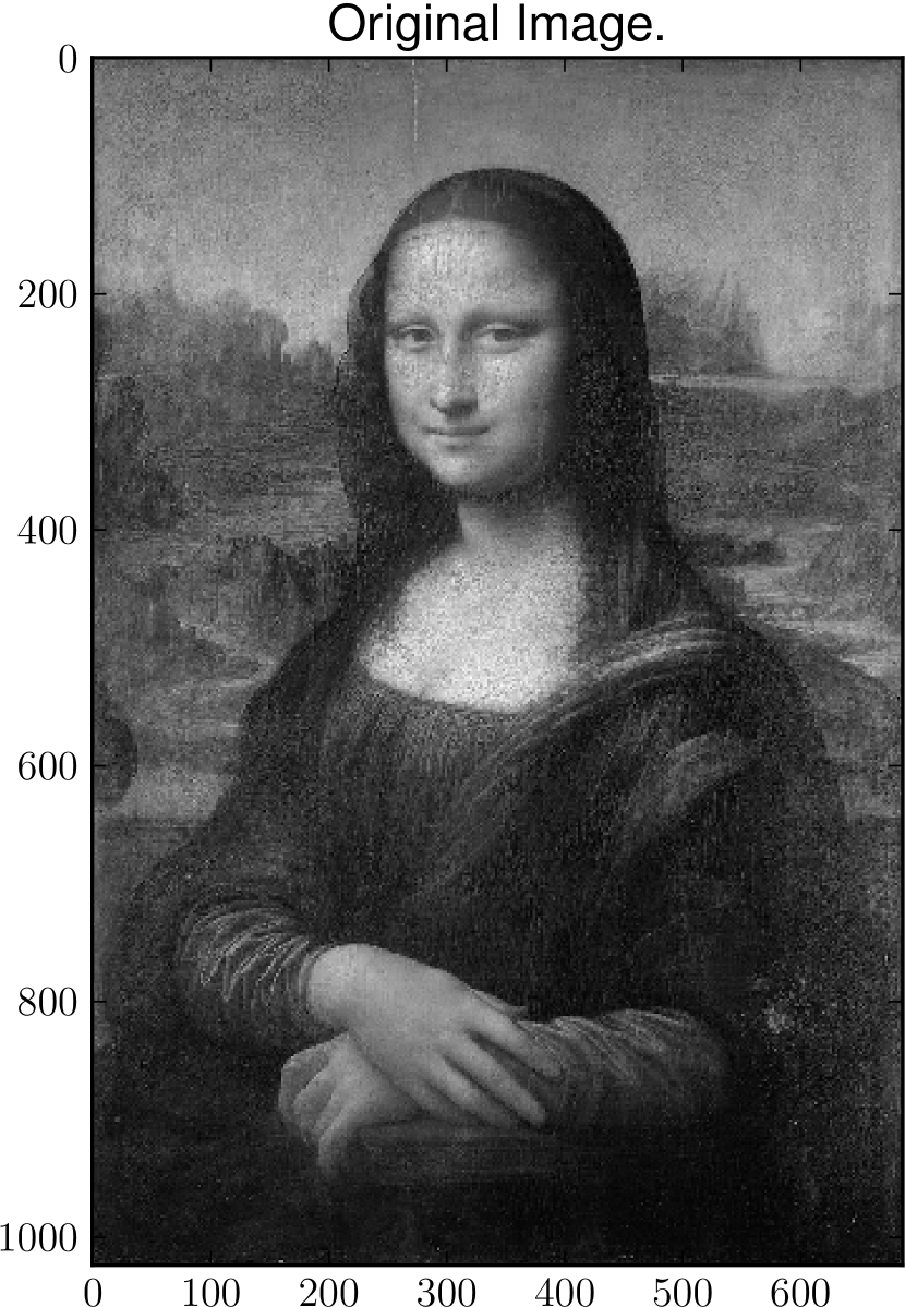
(a) Original Image

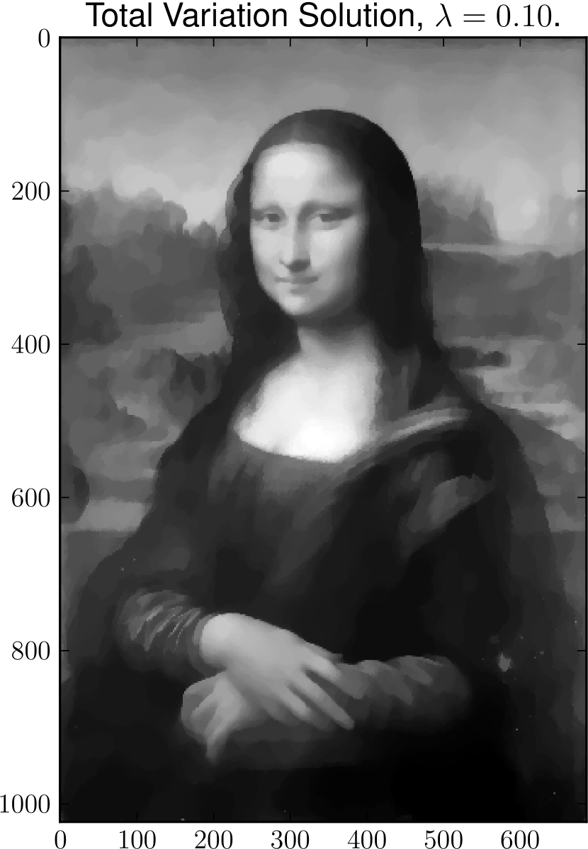
(b) $\operatorname{TV}$ minimized image with $\lambda^{\prime}=0.1$.

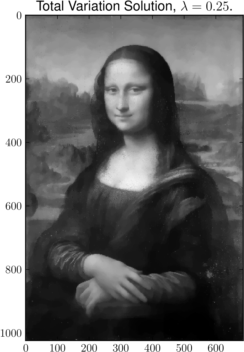
(c) $\operatorname{TV}$ minimized image with $\lambda^{\prime}=0.25$.

Figure 1: An example of Total Variation Minimization for noise removal on Leonardo da Vinci’s Mona Lisa. Different values of the regularization parameter produce different results, with the higher value of $\lambda^{\prime}$ smoothing the image less but removing less of the noise.

The total variation regularizer tends to have a smoothing effect around regions of transition, while also setting similar regions to a constant value. As such, it has proven to be quite effective for removing noise from images and finding the boundaries of sufficiently distinct regions. The locations where the norm of the gradient $\operatorname{TV}(u)$ is nonzero correspond to boundaries of the observed process in which the change is the greatest. A rigorous treatment of the theoretical aspects surrounding using this as a regularization term can be found in Bellettini, Caselles, and Novaga (2002); Ring (2000) and Chan and Esedoglu (2005). A complete and treatment of this topic in practice can be found in a number of surveys, including Darbon and Sigelle (2006); Allard (2007, 2008, 2009); in particular, see Caselles, Chambolle, and Novaga (2011) and Chambolle, Caselles, Cremers, Novaga, and Pock (2010). As our purpose in this work is to present a treatment of the underlying theoretical structures, we refer the reader to one of the above references for use practical image analysis. Still, several points are of statistical interest, which we discuss now.

Several generalizations of the traditional Rudin-Osher-Fatimi model have been proposed for different models of the noise and assumptions about the boundaries of the images. Most of these involve changes to the loss or log-likelihood term but preserve the total variation term as the regularizer. In general, we can treat $u^{*}$ as the estimation of

$$u^{*}=\operatorname*{\;argmin\;}_{u\in{\mathcal{F}}(\Omega)}{\mathcal{L}}(u,f)+\lambda\operatorname{TV}(u)$$ (14)

where ${\mathcal{L}}$ is a smooth convex loss function.

One option is to use $L_{1}$ loss for ${\mathcal{L}}$, namely

$${\mathcal{L}}_{1}=\left\lVert f-u\right\rVert_{\!\text{\hskip 0.35002pt}1},$$ (15)

as a way of making the noise more robust to outliers. This model is explored in Bect et al. (2004); Chan and Esedoglu (2005) and the survey papers above. These perform better under some types of noise and have also become popular (Goldfarb and Yin, 2009).

Similarly, many models for image denoising – often when the image comes from noisy sensing processes in physics, medical imaging, or astronomy – involve using a Poisson likelihood for the observations. Here, we wish to recover a density function where we observe Poisson counts in a number of cells with rate proportional to the true density of the underlying process. Total variation regularization can be employed to deal with low count rates. Here, total variation regularization is used to recover the major structures in the data. In this case, the optimal loss function is given by

$${\mathcal{L}}(u,f)=\int_{\Omega}(u({{\mathbf{x}}})-f({{\mathbf{x}}})\log u({{\mathbf{x}}}))\mathrm{d}{{\mathbf{x}}},\qquad\qquad u\geq 0.$$ (16)

Research on this, including optimization techniques, can be found in Bardsley and Luttman (2009); Bardsley (2008); Sawatzky et al. (2009).

Also of interest in the statistics community, Wunderli (2013) replaces the squared-norm fit penalty in (13) with the quantile regression penalty from Koenker and Bassett Jr (1978), where loss function is replaced with

$${\mathcal{L}}(u,f)={\left\lvert f({{\mathbf{x}}})-u({{\mathbf{x}}})\right\rvert}\times{\left\{\begin{array}[]{ll}1-\beta&f({{\mathbf{x}}})\geq u({{\mathbf{x}}})\\ \beta&f({{\mathbf{x}}})<u({{\mathbf{x}}})\end{array}\right\}}.$$ (17)

for which the author proves the existence, uniqueness, and stability of the solution.

One of the variations of total variation minimization is the Mumford-Shah model. In this model, used primarily for segmenting images, regions of discontinuity are handled explicitly Mumford and Shah (1989). In this model, the energy which is minimized is

$$E(u,\Gamma)=\left\lVert f-u\right\rVert_{\!\text{\hskip 0.35002pt}2}^{\!\text{\hskip 0.35002pt}2}+\int_{\Omega\backslash\Gamma}\left\lVert\nabla\,u\right\rVert_{\!\text{\hskip 0.35002pt}2}^{\!\text{\hskip 0.35002pt}2}\mathrm{d}\mu+v\left\lVert\Gamma\right\rVert$$ (18)

where $\Gamma$ is a collection of curves and $\left\lVert\Gamma\right\rVert$ is the total length of these curves. Thus the function is allowed to be discontinuous on $\Gamma$; these are then taken to be the segmentations of the image. This model has also attracted a lot of attention in the vision community as a way of finding boundaries in the image (Chan and Vese, 2000; Pock et al., 2009; El Zehiry et al., 2007). The Bayesian model of this is as a type of mixture model in which the mean function and noise variance differs between regions (Brox and Cremers, 2007). Unlike general TV regularization, however, it is typically focused exclusively on finding curves for image segmentation, rather than on estimating the original image. While it shares a number of close parallels to our problem, particularly in the graph cut optimizations used (El Zehiry et al., 2007), our method does not appear to generalize to this problem.

The optimization of the total variation problem has garnered a lot of attention as well. An enormous number of approaches have been proposed for this problem. These largely fall into the category of graph based algorithms, active contour methods, or techniques based around partial differential equations. These are discussed in more depth in part 2 of this paper, where we mention them in introducing our approach to the problem.

3 Background and Outline of Main Results

The primary purpose of our work is to present a theory of the underlying structure connecting the optimization of the above models over dependent variables and recent results in combinatorial optimization, particularly submodular function minimization. Our theory connects and makes explicit a number of connections between known results in these fields, many of which we extend in practically relevant ways. The insights gained from our theory motivate a family of novel algorithms for working with these models. Furthermore, we are able to give a complete description of the structure of the regularization path; this result is also completely novel.

One primary practical contribution is the development of methods to efficiently optimize functions of the following form, which we denote as ($\Re_{\!\text{B}}$)

$$\boldsymbol{\mathbf{u}}^{*}(\lambda)=\operatorname*{\;argmin\;}_{\boldsymbol{\mathbf{u}}\in\mathbb{R}^{n}}\left\lVert\boldsymbol{\mathbf{u}}-\boldsymbol{\mathbf{a}}\right\rVert_{\!\text{\hskip 0.35002pt}2}^{\!\text{\hskip 0.35002pt}2}+\lambda\left[\sum_{i}\xi_{i}(u_{i})+\sum_{i,j}w_{ij}{\left\lvert u_{i}-u_{j}\right\rvert}\right], \Re_{\!\text{B}}$$ ()

with ${{\mathbf{a}}}\in\mathbb{R}^{n}$, $\lambda$ is a non-negative regularization parameter, $w_{ij}\geq 0$ controls the regularization of dependent variables, and $\xi_{i}(u_{i})$ is a convex piecewise linear function, possibly the common $L_{1}$ penalty $\xi_{i}(u_{i})={\left\lvert u_{i}\right\rvert}$.

We develop a novel algorithm for ($\Re_{\!\text{B}}$) based on network flows and submodular optimization theory, and completely solve the regularization path as well over $\lambda>0$. The crux of the idea is to construct a collection of graph-based binary partitioning problems indexed by a continuous parameter. With our construction, we show that the points at which each node exactly gives the solution to ($\Re_{\!\text{B}}$). We develop algorithms for this that scale easily to millions of variables, and show that the above construction also unlocks the nature of the regularization path.

These functions arise in two active areas of interest to the statistics and machine learning communities. The first is in the optimization of penalized regression functions where we wish to find

$$\boldsymbol{\mathbf{u}}^{*}(\lambda)=\operatorname*{\;argmin\;}_{\boldsymbol{\mathbf{u}}\in\mathbb{R}^{n}}{\mathcal{L}}{\left(\boldsymbol{\mathbf{u}},\boldsymbol{\mathbf{y}}\right)}+\lambda\left[\sum_{i}\xi_{i}(u_{i})+\sum_{i,j}w_{ij}{\left\lvert u_{i}-u_{j}\right\rvert}\right], \Re_{\!\text{L}}$$ ()

where $\boldsymbol{\mathbf{y}}$ is a collection of observed response and ${\mathcal{L}}(\boldsymbol{\mathbf{u}},\boldsymbol{\mathbf{y}})$ is a smooth, convex log-likelihood term. Throughout our work, we denote this problem as ($\Re_{\!\text{L}}$). In the general case, we handle this problem through the use of the proximal gradient methods, a variant of sub-gradient methods, which we described below. The inner routine involves solving ($\Re_{\!\text{B}}$).

Finally, ($\Re_{\!\text{B}}$) also extends to the continuous variational estimation problem of Total Variation minimization from section 2.2. where we wish to minimize

$$u^{*}=\operatorname*{\;argmin\;}_{{\mathcal{F}}(\Omega)}\left\lVert u-f\right\rVert_{\!\text{\hskip 0.35002pt}2}^{\!\text{\hskip 0.35002pt}2}+\lambda\operatorname{TV}(u) \Re_{\!\text{TV}}$$ ()

where ${\mathcal{F}}(\Omega)$ and $\operatorname{TV}(u)$ are defined in (10) – (13). We show in the second part of our work that this problem can be solved using the methods developed for ($\Re_{\!\text{B}}$). Thus we not only present an efficient algorithm for ($\Re_{\!\text{TV}}$), we also present the first algorithm for finding the full regularization path of this problem.

3.1 Outline

This paper is laid out as followed. The rest of this section presents a survey of the background to the current problem, describing the current state of the research in the relevant areas and laying out the reasons it is of interest to the statistics and machine learning communities.

Section 4 lays out the basic framework connecting network flows, submodular function minimization, and the optimization of ($\Re_{\!\text{B}}$). While some of our results were discovered independently, our theory pulls them together explicitly in a common framework, and provides more direct proofs of their correctness. Additionally, our approach motivates a new algorithm to exactly solve the resulting optimization problem.

Section 5 presents entirely novel results. We extend the basic theory of section 4 using a novel extension lemma to allow for a general size-biasing measure on the different components of the input. The theoretical results are proved for general submodular functions, extending the state-of-the-art in this area. In the context of our problem, we use these results to extend the algorithmic results of section 4. In particular, this opens a way to handle the $\xi_{i}(u_{i})$ term in ($\Re_{\!\text{B}}$) above, significantly extending the results of Mairal et al. (2011) related to section 4.

3.2 Optimization of Regularized Models

Regularized models have gained significant attention in both the statistics and machine learning communities. Intuitively, they provide a way of imposing structure on the problem solution. This facilitates the accurate and tractable estimation of high-dimensional variables or other features, such as change points, that are difficult to do in a standard regression context. Furthermore, these methods have been well studied both from the theoretical perspective – correct estimation is guaranteed under a number of reasonable assumptions – and the optimization perspective – efficient algorithms exist to solve them. Not surprisingly, these approaches have gained significant popularity in both the statistics and machine learning communities. We will describe several relevant examples below.

In the general context, we consider finding the minimum of

$$\gamma(\boldsymbol{\mathbf{u}})={\mathcal{L}}(\boldsymbol{\mathbf{u}},{{\mathbf{y}}})+\lambda\Phi(\boldsymbol{\mathbf{u}}),$$ (19)

where ${\mathcal{L}}(\boldsymbol{\mathbf{u}},{{\mathbf{y}}})$ is a smooth convex Lipshitz loss function, $\Phi(\boldsymbol{\mathbf{u}})$ is a regularization term, and $\lambda\geq 0$ controls the amount of the regularization. In statistical models, ${\mathcal{L}}$ is typically given by the log-likelihood of the model. The regularization term $\Phi(\boldsymbol{\mathbf{u}})$ is required to be convex but is not required to be smooth; in practice it is is often a regularization penalty that enforces some sort of sparseness or structure. A common regularization term is simply the $L_{1}$ norm on $\boldsymbol{\mathbf{u}}$, i.e.

$$\Phi_{1}(\boldsymbol{\mathbf{u}})=\left\lVert\boldsymbol{\mathbf{u}}\right\rVert_{\!\text{\hskip 0.35002pt}1}$$ (20)

which gives the standard LASSO problem proposed in (Tibshirani, 1996) and described in section 2.

A number of algorithms have been proposed for the optimization of this particular problem Friedman et al. (2010); Efron et al. (2004). Most recently, a method using proximal operators has been proposed called the Fast Iterative Soft-Threshold Algorithm (Beck and Teboulle, 2009); this achieves theoretically optimal performance – identical to the $\mathcal{O}{\left({{{\,\!}_{\!\,}^{1}\!\!\!{\diagup}\!\!\!_{k^{2}}^{\!\,}}}\right)}$ lower bound of the convergence rate by iteration of optimization of general smooth, convex functions (Nesterov, 2005). The method is based on the proximal operators we discuss next, and is described in detail, along with theoretical guarantees, in Beck and Teboulle (2009). This is the method that immediately fits with our theoretical results.

3.2.1 Proximal Operators

Proximal gradient methods Nesterov (2007); Beck and Teboulle (2009) are a very general approach to optimizing (19). At a high level, they can be understood as a natural extension of gradient and sub-gradient based methods designed to deal efficiently with the non-smooth component of the optimization. The motivation behind proximal methods is the observation that the objective $\gamma(\boldsymbol{\mathbf{u}})$ is the composition of two convex functions, with the non-smooth part isolated in one of the terms. In this case, the proximal problem takes the form

$$\gamma_{P}(\boldsymbol{\mathbf{u}},{\hat{{\mathbf{u}}}})=f({\hat{{\mathbf{u}}}})+(\boldsymbol{\mathbf{u}}-{\hat{{\mathbf{u}}}})^{T}\nabla\,f({\hat{{\mathbf{u}}}})+\lambda\Phi(\boldsymbol{\mathbf{u}})+\frac{L}{2}\left\lVert\boldsymbol{\mathbf{u}}-{\hat{{\mathbf{u}}}}\right\rVert_{\!\text{\hskip 0.35002pt}2}^{\!\text{\hskip 0.35002pt}2}$$ (21)

where we abbreviate $f(\boldsymbol{\mathbf{u}})={\mathcal{L}}(\boldsymbol{\mathbf{u}},\boldsymbol{\mathbf{y}})$. $L$ is the Lipshitz constant of $f$, which we assume is differentiable. We rewrite this as

$$\gamma_{P}^{\prime}(\boldsymbol{\mathbf{u}},{\hat{{\mathbf{u}}}})=\frac{1}{2}\left\lVert\boldsymbol{\mathbf{u}}-\left[{\hat{{\mathbf{u}}}}-\frac{1}{L}\nabla\,f({\hat{{\mathbf{u}}}})\right]\right\rVert_{\!\text{\hskip 0.35002pt}2}^{\!\text{\hskip 0.35002pt}2}+\frac{\lambda}{L}\Omega(\boldsymbol{\mathbf{u}}).$$ (22)

The minimizing solution of (22) forms the update rule. Intuitively, at each iteration, proximal methods linearize the objective function around the current estimate of the solution, ${\hat{{\mathbf{u}}}}$, then update this with the solution of the proximal problem. As long as (21) can be optimized efficiently, the proximal operator methods give excellent performance.

While this technique has led to a number of algorithmic improvements for simpler regularizers, it has also opened the door to the practical use of much more complicated regularization structures. In particular, there has been significant interest in more advanced regularization structures, particularly ones involving dependencies between the variables. These types of regularization structures are the primary focus of our work.

3.2.2 Related Work

Finally, of most relevance to our work here, is a series of recent papers by Francis Bach and others, namely Bach, Jenatton, Mairal, and Obozinski (2012), Mairal, Jenatton, Obozinski, and Bach (2010), and Mairal, Jenatton, Obozinski, and Bach (2011), that independently discover some of our results. In these papers, combined with the more general work of Bach, Jenatton, Mairal, and Obozinski (2011); Bach (2010b) and Bach (2010a, 2011), several of the results we present here were independently proposed, although from a much different starting point. In particular, he proposes using parametric network flows to solve the proximal operator for $\Phi(\boldsymbol{\mathbf{u}})=\sum_{i,j}w_{ij}{\left\lvert u_{i}-u_{j}\right\rvert}$ and that this corresponds to calculating the minimum norm vector of the associated submodular function. These results are discussed in more detail in section 4.

While our results were discovered independently from these, we extend them in a number of important ways. First, we propose a new algorithm to exactly solve the linear parametric flow problem; this is a core algorithm in these problems. Second, through the use of the weighting scheme proposed in section 5, we develop a way to include general convex linear functions directly in the optimization procedure. This expands the types of regularization terms that can be handled as part of the proximal operator scheme.

3.3 Combinatorial Optimization and Network Flows

The final piece of background work we wish to present forms the last pillar on which our theory is built. Core to the theory and the algorithms is the simple problem of finding the minimum cost partitioning of a set of nodes ${\mathcal{V}}$ in which relationships between these nodes are defined by a graph connecting them. Our results are built on a fundamental connection between a simple combinatorial problem – finding a minimum cost cut on a graph – and the convex optimization problems described in section 3.2.

A fundamental problem in combinatorial optimization is finding the minimum cost cut on a directed graph. This problem is defined by $({\mathcal{V}},{\mathcal{E}},{{\mathbf{c}}},s,t)$, where ${\mathcal{V}}$ is a set of nodes and ${\mathcal{E}}$ is a set of directed edges connecting two nodes in ${\mathcal{V}}$. We consistently use $n$ to denote the number of nodes and, without loss of generality, assume ${\mathcal{V}}={\left\{1,2,...,n\right\}}$, i.e. the nodes are refered to using the first $n$ counting numbers. Similarly, the edges are denoted using pairs of vertices; thus ${\mathcal{E}}\subseteq\left\{(i,j)\,\,\mathbf{:}\,\,i,j\in{\mathcal{V}}\right\}$. Here, $(i,j)$ denotes an edge in the graph going from $i$ to $j$. For an undirected graph, we simply assume that $(i,j)\in{\mathcal{E}}$ if and only if $(j,i)\in{\mathcal{E}}$, and that $c_{ij}=c_{ji}$ for all $i,j\in{\mathcal{V}}$. ${{\mathbf{c}}}$ associates a cost with each of the edges in ${\mathcal{E}}$. I.e. maps from a pair of edges to a non-negative cost, i.e. $c_{ij}\in\mathbb{R}^{+}$ for $(i,j)\in{\mathcal{E}}$.

The letters $s$ and $t$ here denote specific nodes not in the node set ${\mathcal{V}}$. For reasons that will become clear in a moment, $s$ is called the source node and $t$ is called the sink node. We treat $s$ and $t$ as valid nodes in the graph and define the cost associated with an edge from $s$ to $i$ as $c_{si}$; analogously, $c_{it}$ denotes the cost of an edge from $i$ to the sink $t$. These nodes are treated specially in the optimization, however; the minimum cut problem is the problem of finding a cut in the graph separating $s$ and $t$ such that the total cost of the edges cut is minimal. Formally, we wish to find a set $S^{*}\subseteq{\mathcal{V}}$ satisfying

$$S^{*}\in\operatorname*{\;Argmin\;}_{S\subseteq{\mathcal{V}}}\left[\sum_{\begin{subarray}{c}i\in S\\ j\in({\mathcal{V}}\backslash S)\end{subarray}}c_{ij}\right]+\left[\sum_{i\in S}c_{it}\right]+\left[\sum_{i\in{\mathcal{V}}\backslash S}c_{si}\right]$$ (23)

where $\operatorname*{\;Argmin\;}$ with a capital $\operatorname{A}$ returns the set of minimizers, as there may be multiple partitions $S^{*}$ achieving the minimum cost.

The above lays out the basic definitions needed for our work with graph structures. This problem is noteworthy, however, as it can be solved easily by finding the maximal flow on the graph – one of the fundamental dualities in combinatorial optimization is the fact that the cut edges defining the minimum cost partition are the saturated edges in the maximum flow from $s$ to $t$ in the equivalent network flow problem. It is also one of the simplest practical examples of a submodular function, another critical component of our theory. We now describe these concepts.

3.3.1 Network Flows

The network flow problem is the problem of pushing as much “flow” as possible through the graph from $s$ to $t$, where the capacity of each edge is given by the cost mapping ${{\mathbf{c}}}$ above. The significance of this problem is the fact that it map directly to finding the minimum cost partition in a graph (Dantzig and Fulkerson, 1955; Cormen et al., 2001; Kolmogorov and Zabih, 2004). The saturating edges of a maximizing network flow – those edges limiting any more flow from being pushed through the graph – defines the optimal cut in the minimum cut partitioning. This result is one of the most practical results of combinatorial optimization, as many problems map to the partitioning problem above, and one and simple algorithms exist for solving network flow problems.

In the network flow problem, we wish to construct a mapping ${{\mathbf{z}}}$ that represents “flow” from $s$ to $t$. A mapping ${{\mathbf{z}}}$ is a valid flow if, for all nodes in ${\mathcal{V}}$, the flow going into the each node is the same as the flow leaving that node. Specifically,

Definition 3.1 ((Valid) Flow).

Consider a graph ${\mathcal{G}}=({\mathcal{V}},{\mathcal{E}},{{\mathbf{c}}},s,t)$ as described above. Then $z_{ij}$, $i,j\in{\left\{s,t\right\}}\cup{\mathcal{V}}$, is a flow on ${\mathcal{G}}$ if

$$0\leq z_{ij}\leq c_{ij} \,\,\,\forall\,i,j\in{\mathcal{V}}$$ (24)

$$\sum_{i\in{\mathcal{V}}\cup{\left\{s\right\}}}z_{ij}= \sum_{k\in{\mathcal{V}}\cup{\left\{t\right\}}}z_{jk},$$ (25)

where for convenience, we assume that $z_{ii}=0$ and $z_{ij}=c_{ij}=0$ if $(i,j)\notin{\mathcal{E}}$.

Furthermore, we say that an edge $(i,j)$ is saturated if $z_{ij}=c_{ij}$, i.e. the flow on that edge cannot be increased.

Since we frequently talk about flows in a more informal sense, we use the term “valid flow” to reference this formal definition.

It is easy to show that the amount of flow leaving $s$ is the same as the amount of flow leaving $t$, i.e.

$$\text{Total Flow}=\sum_{i\in{\mathcal{V}}}z_{si}=\sum_{i\in{\mathcal{V}}}z_{it}.$$ (26)

this total flow is what we wish to maximize in the maximum flow problem, i.e. we wish to find a maximal flow ${{\mathbf{z}}}^{*}$ such that

$${{\mathbf{z}}}^{*}\in\operatorname*{\;Argmin\;}_{\qquad{{\mathbf{z}}}\,\,\mathbf{:}\,\,{{\mathbf{z}}}\text{ is a valid flow on ${\mathcal{G}}$}\qquad}\sum_{i\in{\mathcal{V}}}z_{si}.$$ (27)

The canonical min-cut-max-flow theorem (Dantzig and Fulkerson, 1955; Cormen et al., 2001) states that the set of edges saturated by all possible maximal flows defines a minimum cut in the sense of (23) above. The immediate practical consequence of this duality is that we are able to find the minimum cut partitioning quickly as fast algorithms exist for finding a maximal flow ${{\mathbf{z}}}^{*}$. We outline one of these below, but first we generalize the idea of a valid flow in two practically relevant ways.

3.3.2 Preflows and Pseudoflows

Two extensions of the idea of a flow ${{\mathbf{z}}}$ on a graph relaxes the equality in the definition of a flow. Relaxing the inequality is key to several algorithms, and forms some interesting connections to the theory we outline. The equality constraint is effectively replaced with an $\operatorname{excess}(\cdot)$ function that gives the excess flow at each node; if the total amount of flow into and out of a node $i$ is equal, then $\operatorname{excess}(i)=0$. Formally,

Definition 3.2 (Preflow).

Consider a graph ${\mathcal{G}}=({\mathcal{V}},{\mathcal{E}},{{\mathbf{c}}},s,t)$ as in definition 3.1. Then $z_{ij}$, $i,j\in{\left\{s,t\right\}}\cup{\mathcal{V}}$, is a flow on ${\mathcal{G}}$ if

$$0\leq z_{ij}\leq c_{ij} \,\,\,\forall\,i,j\in{\mathcal{V}}$$ (28)

$$\sum_{i\in{\mathcal{V}}\cup{\left\{s\right\}}}z_{ij}\geq \sum_{k\in{\mathcal{V}}\cup{\left\{t\right\}}}z_{jk}.$$ (29)

With this definition, we define the $\operatorname{excess}(\cdot)$ function as

$$\operatorname{excess}(i)=\left[\sum_{i\in{\mathcal{V}}\cup{\left\{s\right\}}}z_{ij}\right]-\left[\sum_{k\in{\mathcal{V}}\cup{\left\{t\right\}}}z_{jk}\right].$$ (30)

It is easy to see that if ${{\mathbf{z}}}$ is a preflow, $\operatorname{excess}(i)\geq 0$ for all nodes $i$. Maintaining a valid preflow is one of the key invariants in the common push-relabel algorithm discussed below.

A Pseudoflow is the weakest definition of a flow; it relaxes (29) completely, allowing there to be both excesses and deficits on the nodes of the graph. However, it does add in an additional constraint, namely that all edges connected to the source and sink are saturated. Formally,

Definition 3.3 (Pseudoflow).

Consider a graph ${\mathcal{G}}=({\mathcal{V}},{\mathcal{E}},{{\mathbf{c}}},s,t)$ as in definition 3.1. Then $z_{ij}$, $i,j\in{\left\{s,t\right\}}\cup{\mathcal{V}}$, is a flow on ${\mathcal{G}}$ if

$$0\leq z_{ij}\leq c_{ij} \,\,\,\forall\,i,j\in{\mathcal{V}}$$ (31)

$$z_{si}=c_{si} \,\,\,\forall\,i\in{\mathcal{V}}$$ (32)

$$z_{it}=c_{it} \,\,\,\forall\,i\in{\mathcal{V}}$$ (33)

Note that now the $\operatorname{excess}(i)$ function can be either positive or negative. A pseudoflow has some interesting geometric and algorithmic properties, It was described in Hochbaum (1998) and an efficient algorithm for solving network flows based on pseudoflows was presented in Hochbaum (2008). We mention it here to preview our results in section 4: the pseudoflow matches up directly with the base polytope, one of the fundamental structures in submodular function optimization.

3.3.3 Network Flow Algorithms

Finding the minimum cut or the maximum flow on a network is one of the oldest combinatorial optimization problems, and, as such, it is also one of the most well studied. It would be impossible to detail the numerous algorithms to solve the network flow problem here – Schrijver (2003) lists over 25 survey papers on different network flow algorithms. Many of these are tailored for different types of graphs (sparse vs. dense) and other variations of the problem.

Perhaps the most well-known algorithm for Network flow analysis is the push-relabel method. Variants of it achieve the best known performance guarantees for a number of problems of interest. It is simple to implement; essentially, each node has a specific height associated with it that represents (informally) the number of edges in the shortest unsaturated path to the sink. Each node can have an excess amount of flow from the source. At each iteration, a node with excess either pushes flow along an unsaturated edge to a neighbor with a lesser height, or increments its height. Termination occurs when the source node is incremented to $\left\lvert{{\mathcal{V}}}\right\rvert+1$, where $\left\lvert{{\mathcal{V}}}\right\rvert$ is the number of nodes – at this point, there is no possible path to the sink and the maximum cut can be found. For more information on this, along with other information on this algorithm, see Cormen et al. (2001) or Schrijver (2003). This algorithm runs at the core of our network flow routines. This algorithm is guaranteed to run in polynomial time; in the general case, it runs in $\mathcal{O}{\left(\left\lvert{{\mathcal{V}}}\right\rvert^{2}\left\lvert{{\mathcal{E}}}\right\rvert\right)}$ time, where ${\mathcal{V}}$ is the set of vertices and ${\mathcal{E}}$ is the set of edges. However, it can be improved to $\mathcal{O}{\left(\left\lvert{{\mathcal{V}}}\right\rvert\left\lvert{{\mathcal{E}}}\right\rvert\log(\left\lvert{{\mathcal{V}}^{2}}\right\rvert/\left\lvert{{\mathcal{E}}}\right\rvert)\right)}$ using dynamic tree structures (Schrijver, 2003).

3.3.4 The Parametric Flow Problem

One variation of the regular network flow problem is the parametric flow problem (Gallo et al., 1989). The general parametric flow problem is a simple modification of the maximum flow problem given above, except that now $c_{si}$ is replaced with a monotonic non-decreasing function $c_{si}(\beta)$,

$${{\mathbf{z}}}^{*}(\beta)\in\operatorname*{\;Argmin\;}_{\begin{subarray}{c}{{\mathbf{z}}}\,\,\mathbf{:}\,\,{{\mathbf{z}}}\text{ is a valid flow on ${\mathcal{G}}(\beta)$;}\\ \qquad\text{Capacity of edge $(s,i)$ given by $c_{si}(\beta)$}\qquad\end{subarray}}\sum_{i\in{\mathcal{V}}}z_{si}.$$ (34)

Gallo et al. (1989) showed that this problem could be solved for a fixed sequence $\beta_{1}<\beta_{2}<\cdots<\beta_{m}$ in time proportional to the time of a single run of the network flow problem by exploiting a nestedness property of the solutions. Namely, as $\beta$ increase, the minimum cut of the optimal solution moves closer on the graph to the source. More formally, if $\beta_{1}<\beta_{2}$, then

$$S^{*}(\beta_{1})\subseteq S^{*}(\beta_{2}),$$ (35)

where $S^{*}(\beta)$ is an optimal cut at $\beta$ in the sense of (23).

If $c_{si}(\beta)$ is a linear function with positive slope, we call this problem the the linear parametric flow problem. In sections 4 and 5, we develop an exact algorithm for this problem that does not require a predetermined sequence of $\beta$ to solve. This method is one of the key routines in the algorithms for general optimization.

3.3.5 Connections to Statistical Problems

One of the recent applications of graph partitioning is in finding the minimum energy state of a binary Markov random field. In particular, if we can model the pairwise interactions over binary variables $x_{1},...,x_{n}$ on the graph using unary and pairwise potential functions $E^{1}_{i}(x_{i})$ and $E^{2}_{ij}(x_{i},x_{j})$, then the minimum energy solution can be found using the maximum cut on a specially formulated graph, provided that $E^{2}_{ij}(0,0)+E^{2}_{ij}(1,1)\leq E^{2}_{ij}(0,1)+E^{2}_{ij}(1,0)$ for all $i,j$. This application of network flow solvers has had substantial impact in the computer vision community, where pairwise potential functions satisfying this condition are quite useful.

We discuss the details of this application in section 4, where we start with the theory behind these connections as first building block of our other results. Ultimately, we show that network flow algorithms can be used to solve not only this problem, but the much more general optimization problems described in section 3.2 as well. Through these connections, we hope to bring the power of network flow solvers into more common use in the statistical community.

3.4 Submodular Functions

The problem of finding a minimal partition in a graph is a special case of a much larger class of combinatorial optimization problems called submodular function minimization. Like the problem of finding a minimal-cost partitioning of a graph given in (23), this optimization problem involves finding the minimizing set over a submodular function $f\,\,\mathbf{:}\,\,2^{\mathcal{V}}\mapsto\mathbb{R}$, where $2^{\mathcal{V}}$ denotes the collection of all subsets of a ground set ${\mathcal{V}}$. Given this, $f$ is submodular if, for all sets $S,T\subseteq{\mathcal{V}}$,

$$f(S)+f(T)\geq f(S\cap T)+f(S\cup T).$$ (36)

This condition is seen as the discrete analogue of convexity. It is sufficient to guarantee that a minimizing set $S^{*}$ can be found in polynomial time complexity.

An alternative definition of submodularity involves the idea of diminishing returns (Fujishige, 2005). Specifically $f$ is submodular if and only if for all $S\subseteq T\subset{\mathcal{V}}$, and for all $i\in{\mathcal{V}}\backslash T$,

$$f(S\cup{\left\{i\right\}})-f(S)\leq f(T\cup{\left\{i\right\}})-f(T).$$ (37)

This property is be best illustrated with a simple example. Let $A_{1},A_{2},...,A_{n}\subseteq{\mathcal{A}}$ be $n$ subsets of a larger set ${\mathcal{A}}$, and define

$$f_{\text{coverage}}(S)=\left\lvert{\bigcup_{i\in S}A_{i}}\right\rvert,$$ (38)

so $f_{\text{coverage}}(S)$ measures the coverage of the set $\cup_{i\in S}A_{i}$. In this context, it is easy to see that $f_{\text{coverage}}(S)$ satisfies (37).

$f_{\text{coverage}}(S)$ is an example of a monotone submodular function as adding new elements to $S$ is only going to increase the value of $f_{\text{coverage}}(S)$. However, many practical examples do not fall into this category. In particular, the graph cut problem given in equation (23) above is non-monotone submodular:

$$f_{\text{gc}}(S)=\left[\sum_{\begin{subarray}{c}i\in S\\ j\in({\mathcal{V}}\backslash S)\end{subarray}}c_{ij}\right]+\left[\sum_{i\in S}c_{it}\right]+\left[\sum_{i\in{\mathcal{V}}\backslash S}c_{si}\right].$$ (39)

We examine this particular example in more detail in section 4, where we prove $f_{gc}$ is indeed submodular.

Submodular function optimization has gained significant attention lately in the machine learning community, as many other practical problems involving the sets can be phrased as submodular optimization problems. It has been used for numerous applications in computer vision, language modeling (Lin and Bilmes, 2010, 2012), clustering (Narasimhan, Jojic, and Bilmes, 2005; Narasimhan and Bilmes, 2007), computer vision (Jegelka and Bilmes, 2011, 2010), and many other domains. This field is quite active, both in terms of theory and algorithms, and we contribute some novel results to both areas in section 5.

The primary focus of our work has been developing a further connection between these graph problems and submodular optimization theory. Our approach, however, is the reverse of much of the previous work. Ultimately, we attempted to map the network flow problems back to the submodular optimization problems. Surprisingly, this actually opened the door to several new theoretical results for continuous optimization, and, in particular, to efficient solutions of the optimization problems given in section 2.

3.4.1 Some Formalities

The theory surrounding submodular optimization, and combinatorial optimization in general, is quite deep. Many of the results underlying submodular optimization require a fairly substantial tour of the theory of the underlying structures; good coverage of these results is found in (Fujishige, 2005) and (Schrijver, 2003). Most of these results are not immediately relevant to our work, so we leave them to the interested reader. However, several additional results are needed for some of the proofs we use later.

As with the discussion of problem, we assume that ${\mathcal{V}}={\left\{1,2,3,...,n\right\}}$; our notation intentionally matches that of the minimum cut problem defined above and is consistent throughout our work. We refer to ${\mathcal{V}}$ as the ground set. Formally, $f$ can be restricted to map from a collection of subsets of $2^{\mathcal{V}}$, which we refer to consistently as ${\mathcal{D}}$, with ${\mathcal{D}}\subseteq 2^{\mathcal{V}}$. In the context of submodular functions, ${\mathcal{D}}$ must be closed under union and intersection and include ${\mathcal{V}}$ as an element(Fujishige, 2005). In general, and except for some of our proofs in section 5, ${\mathcal{D}}$ can be thought of as $2^{\mathcal{V}}$.

3.4.2 Submodular Function Optimization

The first polynomial time algorithm for submodular function optimization was described in (Grötschel et al., 1993); it used the ellipsoid method from linear programming (Chvátal, 1983). While sufficient to prove that the algorithm can be solved in polynomial time, it was impractical to use on any real problems. The first strongly polynomial time algorithms – polynomial in a sense that does not depend on the values in the function – were proposed independently in Schrijver (2000) and Iwata, Fleischer, and Fujishige (2001). The algorithm proposed by Schrijver runs in $\mathcal{O}{\left(n^{8}+\gamma n^{7}\right)}$, where $\gamma$ refers to the complexity of evaluating the function. The latter algorithm is $\mathcal{O}{\left(\gamma n^{7}\log n\right)}$, which may be better or worse depending on $\gamma$. The weakly polynomial version of this algorithm runs in $\mathcal{O}{\left(\gamma n^{5}\log M\right)}$, where $M$ is the difference between maximum and minimum function values. Research in this area, however, is ongoing – a strongly polynomial algorithm that runs in $\mathcal{O}{\left(n^{6}+n^{5}\gamma\right)}$ has been proposed by Orlin (2009).

In practice, the minimum norm algorithm – also called the Fujishige-Wolfe Algorithm – is generally much faster, although it does not have a theoretical upper bound on the running time (Fujishige, 2005). We discuss this algorithm in detail, as it forms the basis of our work. However, there are clear cases that occur in practice where this algorithm does not seem to improve upon the more complicated deterministic ones – in Jegelka, Lin, and Bilmes (2011), a running time of $\mathcal{O}{\left(n^{7}\right)}$ was reported. Thus the quest for practical algorithms for this problem continues; it is an active area of research.

Additionally, several other methods for practical optimization have been proposed for general submodular optimization or for special cases that are common in practice. Stobbe and Krause (2010) proposed an efficient method for submodular functions that can be represented as a decomposable sum of smaller submodular functions given by $g_{i}(\left\lvert{U_{i}\cap S}\right\rvert)$, where $g_{i}$ is convex. In this particular case, the function can be mapped to a form that permits the use of nice numerical optimization techniques; however, many submodular functions cannot be minimized using this technique, and it can also be slow (Jegelka et al., 2011). Along with analyzing the deficiencies of existing methods, Jegelka, Lin, and Bilmes (2011) propose a powerful approach that relies on approximating the submodular functions with a sequence of graphs that permit efficient optimization. This method is quite efficient on a number of practical problems, likely because the graph naturally approximates the underlying structure present in many real-world problems.

Most recently, in Iyer, Jegelka, and Bilmes (2013), another practical optimization method is proposed; at its core is a framework for both submodular minimization and maximization based on a notion of discrete sub-gradients and super-gradients of the function. While not having a theoretical upper bound itself, it performs efficiently in practice. This method is also noteworthy in that it can constrain the solution space in which other exact solvers operate, providing substantial speedups.

3.4.3 Geometrical Structures and the Minimum Norm Algorithm

A number of geometrical structures underpin the theory of submodular optimization. In particular, an associated polymatroid is defined as the set of points in $\left\lvert{{\mathcal{V}}}\right\rvert$-dimensional Euclidean space with sums of sets of the dimensions constrained by the function value of the associated set.

For notational convenience, for a vector ${{\mathbf{x}}}\in\mathbb{R}^{n}$ and set $S\subseteq{\mathcal{V}}$, define

$${{\mathbf{x}}}(S)=\sum_{i\in S}x_{i}.$$ (40)

In this way, ${{\mathbf{x}}}(S)$ forms a type of unnormalized set measure.

Now the polymatroid associated with $f$ is defined as

$$P(f)=\left\{{{\mathbf{x}}}\in\mathbb{R}^{\left\lvert{{\mathcal{V}}}\right\rvert}\,\,\mathbf{:}\,\,{{\mathbf{x}}}(S)\leq f(S)\,\,\,\forall\,S\in{\mathcal{D}}\right\},$$ (41)

$P(f)$ is fundamental to the theory behind submodular function optimization.

In our theory, we work primarily with the base of the polymatroid $P(f)$, denoted by $B(f)$. This is the extreme $(\left\lvert{{\mathcal{V}}}\right\rvert-1)$-dimensional face of $P(f)$; it is defined as

$$B(f)=\left\{{{\mathbf{x}}}\in\mathbb{R}^{\left\lvert{{\mathcal{V}}}\right\rvert}\,\,\mathbf{:}\,\,{{\mathbf{x}}}\in P(f),{{\mathbf{x}}}({\mathcal{V}})=f({\mathcal{V}})\right\}.$$ (42)

In the case where the domain ${\mathcal{D}}=2^{\mathcal{V}}$, $B(f)$ is a linear, convex compact set. Thus it is often refered to as the Base Polytope of $f$ as it is compact.

The base $B(f)$ is particularly important for our work, as one of the key results from submodular function optimization is the minimum norm algorithm, which states effectively that sets $S^{*}$ minimizing $f$ are given by the sign of the point in $B(f)$ closest to the origin. This surprising result, while simple to state, takes a fair amount of deep theory to prove for general $f$; we state it here:

Theorem 3.4 ((Fujishige, 2005), Lemma 7.4.).

For submodular function $f$ defined on $2^{\mathcal{V}}$, let

$${{\mathbf{y}}}^{*}=\operatorname*{\;argmin\;}_{{{\mathbf{y}}}\in B(f)}\left\lVert{{\mathbf{y}}}\right\rVert_{\!\text{\hskip 0.35002pt}2}$$ (43)

and let $S_{1}^{*}=\left\{i\,\,\mathbf{:}\,\,y_{i}^{*}<0\right\}$ and $S_{2}^{*}=\left\{i\,\,\mathbf{:}\,\,y_{i}^{*}\leq 0\right\}$. Then both $S_{1}^{*}$ and $S_{2}^{*}$ minimize $f(S)$ over all subsets $S\subseteq{\mathcal{V}}$. Furthermore, for all $S^{\dagger}\subseteq{\mathcal{V}}$ such that $f(S^{\dagger})=\min_{S\in{\mathcal{V}}}f(S)$, $S_{1}^{*}\subseteq S^{\dagger}\subseteq S_{2}^{*}$.

A central aspect of our theory relies on this result. In general, it as one way of working the geometric structure of the problem. It turns out that in the case of graph partitioning, $B(f)$ takes on a particularly nice form. This allows us to very quickly solve the minimum norm problem here. We show the resulting minimum norm vector also gives us the full solution path over weighting by the cardinality of the minimizing set. While this basic result was independently discovered in Mairal, Jenatton, Obozinski, and Bach (2011), our approach opens several doors for theoretical and algorithmic improvements, which we outline in the subsequent sections.

4 The Combinatorial Structure of Dependent Problems

The foundational aspect of our work is the result established in this section, namely an exploration of network flow minimization problems in terms of their geometric representation on the base polytope of a corresponding submodular problem. This representation is not new; it is explored in some depth as an illustrative example in (Fujishige, 2005) and connected to the minimum norm problems in Mairal et al. (2011). Our contribution, however minor, is based on a simple transformation of the original problem that yields a particularly intuitive geometric form. The fruit of this transformation, however, is a collection of novel results of theoretic and algorithmic interest; in particular, we are able to exactly find the optimal $\boldsymbol{\mathbf{u}}^{*}$ over the problem

$$\boldsymbol{\mathbf{u}}^{*}(\lambda)=\operatorname*{\;argmin\;}_{\boldsymbol{\mathbf{u}}\in\mathbb{R}^{n}}\left\lVert\boldsymbol{\mathbf{u}}-\boldsymbol{\mathbf{a}}\right\rVert_{\!\text{\hskip 0.35002pt}2}^{\!\text{\hskip 0.35002pt}2}+\lambda{\sum_{i,j}w_{ij}{\left\lvert u_{i}-u_{j}\right\rvert}}.$$ (44)

Recall that this problem was discussed in depth in section 3.2; here, ${{\mathbf{a}}}\in\mathbb{R}^{n}$ is given, and $\lambda\in\mathbb{R}^{+}$ and the weights $w_{ij}\in\mathbb{R}^{+}$ control the regularization.

In this section, we lay the theoretical foundation of this work, denoting connections to other related or previously known results. The contribution at the end is a strongly polynomial algorithm for the solution of a particular parametric flow problem; this algorithm follows naturally from this representation. In the next section, we extend the theory to naturally allow a convex piecewise-linear function $\xi_{i}(u_{i})$ to be included in (44) to match ($\Re_{\!\text{B}}$).

Before presenting the results for the real-valued optimization of (44), we must first present a number of theoretical results using the optimization over sets ${\mathcal{V}}={\left\{1,2,...,n\right\}}$. We begin with the simplest version of this optimization – finding the minimizing partition of a graph – and extend this result to general submodular functions later.

4.1 Basic Equivalences

We proceed by defining and establishing equivalences between three basic forms of the minimum cut problem on a graph. Recall from section 3.3 that the minimum cut problem is the problem of finding a set $S^{*}\subseteq{\mathcal{V}}$ satisfying

$$S^{*}\in\operatorname*{\;Argmin\;}_{S\subseteq{\mathcal{V}}}\left[\sum_{\begin{subarray}{c}i\in S\\ j\in({\mathcal{V}}\backslash S)\end{subarray}}c_{ij}\right]+\left[\sum_{i\in S}c_{it}\right]+\left[\sum_{i\in{\mathcal{V}}\backslash S}c_{si}\right].$$ (45)

As we mentioned earlier, several other important problems can be reduced to this form; in particular, finding the lowest energy state of a binary Markov random field, when the pairwise potential functions satisfy the submodularity condition, is equivalent to this problem. Our task now is to make this explicit.

We here show equivalences between three versions of the problem. The first is ${\mathcal{P}}_{E}$, which gives the standard energy minimization formulation, i.e. finding the MAP estimate of

$$p({{\mathbf{x}}})\propto\exp\!\left[\sum_{(i,j)\in{\mathcal{E}}}E^{2}_{ij}(x_{i},x_{j})+\sum_{i\in{\mathcal{V}}}E^{1}_{i}(x_{i})\right],\qquad{{\mathbf{x}}}\in{\left\{0,1\right\}}^{n}$$ (46)

which is equivalent to finding

$${{\mathbf{x}}}^{*}\in\operatorname*{\;Argmin\;}_{{{\mathbf{x}}}\in{\left\{0,1\right\}}^{n}}\sum_{(i,j)\in{\mathcal{E}}}E^{2}_{ij}(x_{i},x_{j})+\sum_{i\in{\mathcal{V}}}E^{1}_{i}(x_{i}).$$ (47)

${\mathcal{P}}_{Q}$ gives the formulation as a quadratic binary minimization problem; here, the problem is to find ${{\mathbf{x}}}\in{\left\{0,1\right\}}^{n}$ that minimizes ${{\mathbf{x}}}^{T}{{\mathbf{Q}}}{{\mathbf{x}}}$ for an $n\times n$ matrix ${{\mathbf{Q}}}$. This version forms a convenient form that simplifies much of the notation in the later proofs. Finally, we show it is equivalent to the classic network flow formulation, denoted ${\mathcal{P}}_{N}$. This states the original energy minimization problem as the minimum $st$-cut on a specially formulated graph structure. The equivalence of these representations is well known (Kolmogorov and Zabih, 2004) and widely used, particularly in computer vision applications. We here present a different parametrization of the problem which anticipates the rest of our results.

The other unique aspect of our problem formulation is the use of a size biasing term; specifically, we add a term $\beta\left\lvert{S}\right\rvert$ to the optimization problem, where $\beta\in\mathbb{R}$ can be positive or negative. This term acts similarly to a regularization term in how it influences the optimization, but to think of it this way would lead to confusion as the true purpose of this formulation is revealed later in this section – ultimately, we show equivalence between the values of $\beta$ at which the set membership of a node flips and the optimal values of the continuous optimization problem of ($\Re_{\!\text{B}}$).

Theorem 4.1.

Let $G={\mathcal{V}},{\mathcal{E}})$ be an undirected graph, where ${\mathcal{V}}$ is the set of vertices (assume ${\mathcal{V}}={\left\{1,...,n\right\}}$) and ${\mathcal{E}}\subseteq\left\{(i,j)\,\,\mathbf{:}\,\,i,j\in{\mathcal{V}}\right\}$ is the set of edges. Without loss of generality, assume that $i<j\,\,\,\forall\,(i,j)\in{\mathcal{E}}$. Define ${\mathcal{S}}_{E}^{*}(\beta)$, ${\mathcal{S}}_{Q}^{*}(\beta)$, and ${\mathcal{S}}_{N}^{*}(\beta)$ as the sets of optimizing solutions to the following three problems, respectively:

Energy Minimization: ${\mathcal{P}}_{E}(\beta)$.

Given an energy function ${{\mathbf{E}}}_{1}={\left(E_{i}(x_{i})\,\,\mathbf{:}\,\,i\in{\mathcal{V}}\right)}$ defined for each vertex $i\in{\mathcal{V}}$ and a pairwise energy function ${{\mathbf{E}}}_{2}={\left(E_{i,j}(x_{i},x_{j})\,\,\mathbf{:}\,\,(i,j)\in{\mathcal{E}}\right)}$ defined for each edge $(i,j)\in{\mathcal{E}}$, with $E_{ij}(0,0)+E_{ij}(1,1)\leq E_{ij}(0,1)+E_{ij}(1,0)$, let

$${{\mathbf{X}}}^{*}(\beta)=\operatorname*{\;Argmin\;}_{{{\mathbf{x}}}\in{\left\{0,1\right\}}^{n}}\sum_{i\in{\mathcal{V}}}{\left(E_{i}(x_{i})-\beta x_{i}\right)}+\sum_{\begin{subarray}{c}(i,j)\in{\mathcal{E}}\\ i<j\end{subarray}}E_{ij}(x_{i},x_{j})$$ (48)

and let

$${\mathcal{S}}_{E}^{*}(\beta)=\bigl{\{}\left\{i\,\,\mathbf{:}\,\,x^{*}_{i}=1\right\}\,\,\mathbf{:}\,\,{{\mathbf{x}}}^{*}\in{{\mathbf{X}}}^{*}(\beta)\bigr{\}}.$$ (49)

Quadratic Binary Formulation: ${\mathcal{P}}_{Q}(\beta)$.

Given ${{\mathbf{E}}}_{1}$ and ${{\mathbf{E}}}_{2}$ as in ${\mathcal{P}}_{E}(\beta)$, define the $n\times n$ matrix ${{\mathbf{Q}}}=[q_{ij}]$ as:

$$q_{ij} ={\left\{\begin{array}[]{ll}E_{ij}(1,1)+E_{ij}(0,0)-E_{ij}(0,1)-E_{ij}(1,0)&i<j\\ 0&\text{otherwise}\end{array}\right.}$$ (52)

$$q_{ii} =(E_{i}(1)-E_{i}(0))+\!\!\!\!\sum_{i^{\prime}<i\,\,\mathbf{:}\,\,(i^{\prime},i)\in{\mathcal{E}}}\!\!\!\!(E_{i^{\prime},i}(0,1)-E_{i^{\prime},i}(0,0))+\!\!\!\!\sum_{j>i\,\,\mathbf{:}\,\,(i,j)\in{\mathcal{E}}}\!\!\!\!(E_{ij}(1,0)-E_{ij}(0,0)).$$ (53)

Suppose $q_{ij}\leq 0$ for $i\neq j$, and let

$${{\mathbf{X}}}^{*}=\operatorname*{\;Argmin\;}_{{{\mathbf{x}}}\in{\left\{0,1\right\}}^{n}}{{\mathbf{x}}}^{T}({{\mathbf{Q}}}-\beta{{\mathbf{I}}})\,{{\mathbf{x}}},$$ (54)

and let

$${\mathcal{S}}_{Q}^{*}(\beta)=\bigl{\{}\left\{i\,\,\mathbf{:}\,\,x^{*}_{i}=1\right\}\,\,\mathbf{:}\,\,{{\mathbf{x}}}^{*}\in{{\mathbf{X}}}^{*}(\beta)\bigr{\}}.$$ (55)

Minimum Cut Formulation: ${\mathcal{P}}_{N}(\beta)$.

Let ${\mathcal{G}}^{\prime}=({\mathcal{V}}^{\prime},{\mathcal{E}}^{\prime})$ be an augmented undirected graph with ${\mathcal{V}}^{\prime}={\mathcal{V}}\cup{\left\{s,t\right\}}$, where $s$ and $t$ represent source and sink vertices, respectively, and ${\mathcal{E}}^{\prime}={\mathcal{E}}\cup\left\{(s,i)\,\,\mathbf{:}\,\,i\in{\mathcal{V}}\right\}\cup\left\{(i,t)\,\,\mathbf{:}\,\,i\in{\mathcal{V}}\right\}\cup\left\{(j,i)\,\,\mathbf{:}\,\,(i,j)\in{\mathcal{E}}\right\}$. Define capacities $c_{ij}$, $(i,j)\in{\mathcal{E}}$ on the edges as:

$$c_{si}=c_{si}(\beta) =\left[a_{i}(\beta)\right]^{+} c_{ji}=c_{ij} =-\frac{q_{ij}}{2},\;i<j c_{jt}=c_{jt}(\beta) =\left[a_{j}(\beta)\right]^{-}$$ (56)

where

$$a_{i}(\beta)=\frac{1}{2}\sum_{i^{\prime}:i^{\prime}<i}q_{i^{\prime},i}+(q_{ii}-\beta)+\frac{1}{2}\sum_{j\,\,\mathbf{:}\,\,ie<j}q_{ij}.$$ (57)

Then the set of minimum cut solutions ${\mathcal{S}}_{N}^{*}(\beta)$ is given by

$${\mathcal{S}}_{N}^{*}(\beta)=\operatorname*{\;Argmin\;}_{\begin{subarray}{c}S\subset{\mathcal{V}}^{\prime}\\ s\in S,\,t\in{\mathcal{V}}^{\prime}\backslash S\;\;\end{subarray}}\sum_{(i,j)\in\delta(S,{\mathcal{V}}^{\prime}\backslash S)}c_{ij}(\beta).$$ (58)

Then ${\mathcal{P}}_{E}(\beta)$, ${\mathcal{P}}_{Q}(\beta)$, and ${\mathcal{P}}_{N}(\beta)$ are equivalent in the sense that any minimizer of one problem is also a minimizer of the others; specifically,

$${\mathcal{S}}_{E}^{*}(\beta)={\mathcal{S}}_{Q}^{*}(\beta)={\mathcal{S}}_{N}^{*}(\beta)$$ (59)

Proof.

A reformulation of known results (Kolmogorov and Zabih, 2004), but given in section A for convenience. ∎

The primary consequence of this theorem is that solving the energy minimization problem can be done efficiently and exactly due to several types of excellent network flow solvers that make solving problems with millions of nodes routine (Boykov and Kolmogorov, 2004; Cormen et al., 2001; Schrijver, 2003). Because of this, numerous applications for graphcuts have emerged in recent years for computer vision and machine learning. Our purpose, in part, is to expand the types of problems that can be handled with network flow solvers, and problems of interest in statistics in particular.

In our work, we alternate frequently between the above representations. For construction, the energy minimization problem is nicely behaved. In the theory, we typically find it easiest to work with the quadratic binary problem formulation due to the algebraic simplicity of working in that form. Again, however, each of these is equivalent; when it does not matter which form we use, we refer to the problem an solution set as ${\mathcal{S}}^{*}(\beta)$ and ${\mathcal{P}}(\beta)$ respectively.

4.1.1 Connections to Arbitrary Network Flow Problems

While theorem 4.1 lays out the equivalence between ${\mathcal{P}}_{E}(\beta)$ and ${\mathcal{P}}_{Q}(\beta)$ and a specific form of network flow problem ${\mathcal{P}}_{N}(\beta)$, for completeness we show that any network flow problem can be translated into the form ${\mathcal{P}}_{N}(\beta)$ and thus ${\mathcal{P}}_{E}(\beta)$ and ${\mathcal{P}}_{Q}(\beta)$. The two distinguishing aspects of ${\mathcal{P}}_{N}(\beta)$ are the facts that each node is connected to either the source or the sink, and that all the edges are symmetric, i.e. $c_{ij}=c_{ji}$ for all $i\neq j$. It is thus sufficient to show that an arbitrary flow problem can be translated to this form. For conciseness, assume that $\beta=0$; the results can be adapted for other $\beta$ easily.

Theorem 4.2.

Any minimum cut problem on an arbitrary, possibly directed graph can be formulated as a quadratic binary problem of the form ${\mathcal{P}}_{Q}(\beta=0)$ as follows:

1. For all edges $(i,j)$ such that $c_{ij}>c_{ji}$, add a path $s\rightarrow j\rightarrow i\rightarrow t$ with capacity $c_{ij}-c_{ji}$. That edge is now undirected in the sense that both directions have the same capacity, and the edges in the minimum cut are unchanged, as these paths will simply be eliminated by flow along that path.

2. Set $q_{ij}=c_{ij}$ for $i<j$ and $q_{ij}=0$ for $i>j$.

3. Given $q_{ij}$, set $q_{ii}=(c_{si}-c_{it})-2\left[\sum_{i^{\prime}:i^{\prime}<i}q_{i^{\prime},i}+\sum_{j\,\,\mathbf{:}\,\,i<j}q_{ij}\right].$

Using these steps, any minimum cut problem can be translated to ${\mathcal{P}}_{Q}$ in the sense that the set of minimizing solutions is identical.

Proof.

Network flows are additive in the sense that increasing or decreasing the capacity of each edge in any path from $s$ to $t$ by a constant amount does not change the set of minimizing solutions of the resulting problem, even if new edges are added (Cormen et al., 2001; Schrijver, 2003). Thus step (1) is valid. The rest follows from simple algebra. ∎

4.2 Network Flows and Submodular Optimization

Recall from section 3.4 that the minimum cut problem is a subclass of the more general class of submodular optimization problems. In the context of ${\mathcal{P}}_{Q}(\beta)$, it is easy to state a direct proof of this fact, additionally showing that here the submodularity of the pairwise terms is also necessary for general submodularity.

Theorem 4.3.

The minimization problem ${\mathcal{P}}_{Q}(\beta)$ can be expressed as minimization of a function $f_{\beta}\,\,\mathbf{:}\,\,2^{\mathcal{V}}\mapsto\mathbb{R}$, with

$$f_{\beta}(S)=\sum_{\begin{subarray}{c}i<j\\ i,j\in S\end{subarray}}q_{ij}+\sum_{i\in S}(q_{ii}-\beta).$$ (60)

Then $f_{\beta}$ is submodular if and only if $q_{ij}\leq 0\,\,\,\forall\,i,j\in S,i<j$.

Proof.

One immediate proof of the if part follows from the fact that ${\mathcal{P}}_{Q}(\beta)$ can be expressed as the sum of submodular pairwise potential terms, and the sum of pairwise submodular functions is also submodular (Fujishige, 2005). The direct proof, including both directions, is a simple reformulation of known results see (Kolmogorov and Zabih, 2004), but given in section A on page A for convenience. ∎

4.2.1 Geometric Structures

We are now ready to present the theory that explicitly describes the geometry of ${\mathcal{P}}_{Q}(\beta)$, which extends to both ${\mathcal{P}}_{E}(\beta)$ and ${\mathcal{P}}_{N}(\beta)$, in the context of submodular function optimization. This theory is not new; several abstract aspects of it have been thoroughly explored by Schrijver (2003) and Fujishige (2005). In our case, however, the exact form of the problem presented in theorem 4.1 was carefully chosen to yield nice properties when this connection is made explicit. From these, a number of desirable properties follow immediately.

The rest of this section is arranged as follows. First, we show that the base polytope $B(f_{\beta})$ is a reduction of all pseudoflows (see definition 3.3) on the form of the cut problem ${\mathcal{P}}_{N}(\beta)$ from theorem 4.1. $B(f_{\beta})$, described in section 3.4, has special characteristics for our purposes, as the minimum norm algorithm described in section 3.4 provides a convenient theoretical tool to examine the structure of ${\mathcal{P}}_{Q}(\beta)$. Our key result is to show that the minimum norm vector – the $L_{2}$-projection of the origin onto $B(f_{\beta})$ – depends on $\beta$ only through a simple, constant shift. Thus this vector allows us to immediately compute the minimum cut directly for any $\beta$, and we are thus able to compute the minimum cut solution as well for any $\beta$ as well.

Theorem 4.4 (Structure of $B(f_{\beta})$).

Let $f_{\beta}$ be defined in theorem 4.3 (60), and let

$${\mathcal{A}}=\left\{{{\boldsymbol{\alpha}}}\in{\mathcal{M}}_{n\times n}\,\,\mathbf{:}\,\,{\left\{\begin{array}[]{ll}{\left\lvert\alpha_{ij}\right\rvert}\leq{\left\lvert q_{ij}\right\rvert}&i<j\\ \alpha_{ij}=0&\text{otherwise}\end{array}\right.}\right\}.$$ (61)

Let $r_{i}({{\boldsymbol{\alpha}}})$, $i=1,...,n$, be defined as follows:

$$r_{i}({{\boldsymbol{\alpha}}})=q_{ii}+\frac{1}{2}\sum_{i^{\prime}<i}{\left(q_{i^{\prime},i}+\alpha_{i^{\prime}i}\right)}+\frac{1}{2}\sum_{j\,\,\mathbf{:}\,\,i<j}{\left(q_{ij}-\alpha_{ij}\right)},$$ (62)

and denote ${{\mathbf{r}}}({{\boldsymbol{\alpha}}})=(r_{1}({{\boldsymbol{\alpha}}}),...,r_{n}({{\boldsymbol{\alpha}}}))\in\mathbb{R}^{n}$. Then the base of the polymatroid associated with $f_{\beta}$, $B(f_{\beta})$, is given by

$$B(f_{\beta})=\left\{{{\mathbf{r}}}({{\boldsymbol{\alpha}}})-\beta\,\,\mathbf{:}\,\,{{\boldsymbol{\alpha}}}\in{\mathcal{A}}\right\},$$ (63)

and the full polymatroid polytope is given by

$$P(f_{\beta})=\left\{{{\mathbf{y}}}\,\,\mathbf{:}\,\,y_{i}\leq y^{\prime}_{i}\,\,\,\forall\,i\text{ for some }{{\mathbf{y}}}^{\prime}\in B(f_{\beta})\right\}.$$ (64)

Proof.

Proceeds with straightforward albeit tedious algebra. Proved in section A on page A.

∎

In light of this, the minimum norm problem on the graph structure is as follows. The immediate corollary to the min-norm theorem is that ${{\boldsymbol{\alpha}}}^{*}(\beta)$ yields the optimum cut $S^{*}(\beta)$ of the corresponding network flow problem, ${\mathcal{P}}_{N}(\beta)$:

Theorem 4.5 (Minimum Norm Formulation of ${\mathcal{P}}_{N}(\beta)$).

Let ${\mathcal{A}}$ and ${{\mathbf{r}}}({{\boldsymbol{\alpha}}})$ be given by equations (61) and (62), respectively. Then the min-norm problem ${\mathcal{P}}_{N}(\beta)$ associated with ${\mathcal{P}}_{Q}(\beta)$ is defined by

$${{\boldsymbol{\alpha}}}^{*}(\beta)=\operatorname*{\;argmin\;}_{{{\boldsymbol{\alpha}}}\in{\mathcal{A}}}\left\lVert{{\mathbf{r}}}({{\boldsymbol{\alpha}}})-\beta\right\rVert_{\!\text{\hskip 0.35002pt}2}$$ (65)

Then any optimal cut $S^{*}(\beta)$ solving ${\mathcal{P}}_{G}(\beta)$, as given in theorem 4.1, satisfies:

$$\left\{i\in{\mathcal{V}}\,\,\mathbf{:}\,\,r_{i}({{\boldsymbol{\alpha}}}^{*}(\beta))<\beta\right\}\subseteq S^{*}(\beta)\subseteq\left\{i\in{\mathcal{V}}\,\,\mathbf{:}\,\,r_{i}({{\boldsymbol{\alpha}}}^{*}(\beta))\leq\beta\right\}.$$ (66)

Proof.

Follows immediately from theorems 4.1 and 4.3 characterizing the cut problem as a submodular function optimization problem, theorem 4.4 describing the structure of this problem, and theorem 3.4 to characterize the solution. ∎

The optimal ${{\boldsymbol{\alpha}}}^{*}$ in the above formulation has some surprising consequences that motivate the rest of our results. In particular, we show that the optimal ${{\boldsymbol{\alpha}}}^{*}$ in equation (65) is independent of $\beta$; this is the key observation that allows us to find the entire regularization path over $\beta$. Formally, this result is given in theorem 4.9. However, we need other results first.

4.2.2 Connection to Flows

The representation in terms of ${{\boldsymbol{\alpha}}}$ is significant partly as the values of ${{\boldsymbol{\alpha}}}$ effectively form a pseudoflow in the sense of Hochbaum (2008) (see section 3.3.2). Recall that a pseudoflow extends the concept of a flow by allowing all the nodes to have both excesses and deficits. In addition, a pseudoflow assumes that all edges from the source to nodes in the graph are saturated, possibly creating excesses at these nodes, and all edges connected to the sink are similarly saturated, possibly creating deficits at these nodes.

Theorem 4.6.

Consider the problem ${\mathcal{P}}_{N}(\beta)$. For any $\alpha_{ij}\in\mathbb{R}$, with $(i,j)\in{\mathcal{E}}$, let $\alpha_{ij}$ represent the flow on each edge $c_{ij}$, with $\alpha_{ij}>0$ indicating flow from $i$ to $j$, and $\alpha_{ij}<0$ indicating flow from $j$ to $i$. Then ${{\boldsymbol{\alpha}}}\in{\mathcal{A}}$ defines a pseudoflow on the graph structure indexed by ${\mathcal{A}}$. Furthermore, $r_{i}({{\boldsymbol{\alpha}}})-\beta=\operatorname{excess}(i)$ is the (possibly negative) excess at node $i$ in the sense of (30).

Proof.

The pseudoflow condition that all edges from the source node and to the sink node are saturated is immediately implied by the fact that $r_{i}(\boldsymbol{\mathbf{0}})-\beta w_{i}=(c_{si}-c_{it})-\beta$. The flow conditions, then follow from the edge capacity being $c_{ij}=c_{ji}=-q_{ij}$ and $-{\left\lvert q_{ij}\right\rvert}\leq\alpha_{ij}\leq{\left\lvert q_{ij}\right\rvert}$. ∎

Corollary 4.7.

Every pseudoflow on the graph defined by theorem 4.1 maps to a point in the base polytope $B(f_{\beta})$, and every point in $B(f_{\beta})$ is given by at least one pseudoflow.

Proof.

Follows immediately from theorem 4.6. ∎

4.3 Structure of the Complete Solution

The theorem above has a number of important consequences detailed in the next few sections. The most immediate consequence comes when we consider the structure of the optimal solution of the minimum norm algorithm specialized to the network flow problem ${\mathcal{P}}_{N}(\beta)$; this effectively allows us to derive a way of solving ${\mathcal{P}}_{N}(\beta)$ for all $\beta$.

Lemma 4.8 (Optimal solutions to ${\mathcal{P}}_{N}(\beta)$).

Then ${{\boldsymbol{\alpha}}}^{*}$ is an optimal solution to ${\mathcal{P}}_{N}(\beta)$ if and only if for all $i,j$, $i<j$, the following condition holds:

$${\left\{\begin{array}[]{ll}\qquad\alpha^{*}_{ij}={\left\lvert q_{ij}\right\rvert}&\qquad\iff\qquad r_{i}({{\boldsymbol{\alpha}}}^{*})\geq r_{j}({{\boldsymbol{\alpha}}}^{*})\\ -{\left\lvert q_{ij}\right\rvert}\leq\alpha^{*}_{ij}\leq{\left\lvert q_{ij}\right\rvert}&\qquad\iff\qquad r_{i}({{\boldsymbol{\alpha}}}^{*})=r_{j}({{\boldsymbol{\alpha}}}^{*})\\ \qquad\alpha^{*}_{ij}=-{\left\lvert q_{ij}\right\rvert}&\qquad\iff\qquad r_{i}({{\boldsymbol{\alpha}}}^{*})\leq r_{j}({{\boldsymbol{\alpha}}}^{*})\end{array}\right\}}.$$ (67)

In particular, the optimum value of ${{\boldsymbol{\alpha}}}^{*}$ in this case is independent of $\beta$.

Proof.

First, ${\mathcal{A}}$ is convex as each dimension $\alpha_{ij}$ is bounded independently. Thus the objective of ${\mathcal{P}}_{N}(\beta)$ is minimizing a convex function over a convex domain. Therefore, it suffices to prove that equation (67) can be satisfied if and only if ${{\boldsymbol{\alpha}}}^{*}$ is a local minimum of $\left\lVert{{\mathbf{r}}}({{\boldsymbol{\alpha}}})-\beta\right\rVert_{\!\text{\hskip 0.35002pt}2}^{2}$. As $\left\lVert{{\mathbf{r}}}({{\boldsymbol{\alpha}}})-\beta\right\rVert_{\!\text{\hskip 0.35002pt}2}^{2}$ is differentiable w.r.t. ${{\boldsymbol{\alpha}}}$, this is equivalent to showing that either the gradient is $0$ or ${{\boldsymbol{\alpha}}}^{*}$ is on the boundary of ${\mathcal{A}}$ and all coordinate-wise derivatives point outside the domain ${\mathcal{A}}$.

First, define $g_{ij}({{\boldsymbol{\alpha}}})$ as the gradient of $\left\lVert{{\mathbf{r}}}({{\boldsymbol{\alpha}}})-\beta\right\rVert_{\!\text{\hskip 0.35002pt}2}^{2}$ w.r.t. $\alpha_{ij}$:

$$g_{ij}({{\boldsymbol{\alpha}}}) =\frac{\partial\,}{\partial\alpha_{ij}}\left\lVert{{\mathbf{r}}}({{\boldsymbol{\alpha}}})-\beta\right\rVert_{\!\text{\hskip 0.35002pt}2}^{2}=2\sum_{k}(r_{k}({{\boldsymbol{\alpha}}})-\beta)\frac{\partial\,}{\partial\alpha_{ij}}r_{k}({{\boldsymbol{\alpha}}})$$ (68)

Now

$$\frac{\partial\,}{\partial\alpha_{ij}}r_{k}({{\boldsymbol{\alpha}}})={\left\{\begin{array}[]{ll}1&k=i\\ -1&k=j\\ 0&\text{otherwise}\end{array}\right.}.$$ (69)

Thus,

$$g_{ij}({{\boldsymbol{\alpha}}}) =2\left[{\left(r_{i}({{\boldsymbol{\alpha}}})-\beta\right)}-{\left(r_{j}({{\boldsymbol{\alpha}}})-\beta\right)}\right]$$ (70)

$$=2\left[r_{i}({{\boldsymbol{\alpha}}})-r_{j}({{\boldsymbol{\alpha}}})\right],$$ (71)

and the following condition holds for all ${{\boldsymbol{\alpha}}}$:

$${\left\{\begin{array}[]{ccc}{g_{ij}({{\boldsymbol{\alpha}}})<0}&\iff&\quad{r_{i}({{\boldsymbol{\alpha}}})>r_{j}({{\boldsymbol{\alpha}}})}\\ {g_{ij}({{\boldsymbol{\alpha}}})=0}&\iff&\quad{r_{i}({{\boldsymbol{\alpha}}})=r_{j}({{\boldsymbol{\alpha}}})}\\ {g_{ij}({{\boldsymbol{\alpha}}})>0}&\iff&\quad{r_{i}({{\boldsymbol{\alpha}}})<r_{j}({{\boldsymbol{\alpha}}})}\end{array}\right\}}.$$ (72)

Matching these conditions to those in (67) shows that ${{\boldsymbol{\alpha}}}^{*}$ as given defines a local, and thus global, optimum of ${\mathcal{P}}_{N}(\beta)$. In particular, note that this criterion is independent of $\beta$, completing the proof. ∎

4.3.1 Invariance to $\beta$

The invariance of the optimal ${{\boldsymbol{\alpha}}}^{*}$ to $\beta$ allows us to characterize the solution space of optimal cuts as the level sets of ${{\mathbf{r}}}({{\boldsymbol{\alpha}}}^{*})$. The core result, as well as our algorithm, is based on this intuition.

Theorem 4.9 ().

1. ${{\boldsymbol{\alpha}}}^{*}$ is the optimal solution to (65) if and only if for all $\beta\in\mathbb{R}$, all optimal cuts $S^{*}_{\beta}\in{\mathcal{S}}^{*}(\beta)$ for ${\mathcal{P}}(\beta)$ satisfy

   $$U_{1}(\beta)=\left\{i\in{\mathcal{V}}\,\,\mathbf{:}\,\,r_{i}({{\boldsymbol{\alpha}}}^{*})<\beta\right\}\subseteq S^{*}_{\beta}\subseteq\left\{i\in{\mathcal{V}}\,\,\mathbf{:}\,\,r_{i}({{\boldsymbol{\alpha}}}^{*})\leq\beta\right\}=U_{2}(\beta)$$ (73)

2. Furthermore, for all $\beta$, $U_{1}(\beta)$ is the unique smallest minimizer of ${\mathcal{P}}(\beta)$ and $U_{2}(\beta)$ is the unique largest minimizer.

Proof.

Part (I) follows as a direct consequence of theorem 4.5 and the invariance of the minimum norm problem to changes in $\beta$ as given in lemma 4.8. Part (II) is then an immediate consequence of the minimum norm algorithm. ∎

This theorem is intuitively important as the key values that permit a connection to the continuous problems are values of $\beta$ at which the membership of the different nodes change. This theorem tells us that these points are given by the values of the minimum norm vector, here given as ${{\mathbf{r}}}({{\boldsymbol{\alpha}}}^{*})$.

4.3.2 Monotonicity

One immediate corollary of theorem 4.9 is a monotonicity property on the optimal sets, used in the continuous optimization theory we present later:

Corollary 4.10.

Let $\beta_{1}<\beta_{2}$. Then for all $S^{*}_{1}\in{\mathcal{S}}^{*}(\beta_{1})$ and $S^{*}_{2}\in{\mathcal{S}}^{*}(\beta_{2})$,

$$S^{*}_{1}\subset S^{*}_{2}.$$ (74)

Proof.

Follows immediately from the equivalence of the optimizing sets to the level sets of the minimum norm vector given in theorem 4.9. ∎

4.4 Beyond Network Flows

Theorem 4.9 above was discovered independently for the full case of general submodular functions by Nagano et al. (2011). There, the authors similarly showed that the level sets of the minimum norm algorithm give the solutions for the $f(S)-\beta\left\lvert{S}\right\rvert$ problem. While the approach those authors take is different and more involved, we give a shorter, alternative proof. We use a simple argument following from the fact that $B(f)$ constrains the minimum norm vector ${{\mathbf{y}}}$ to a constant total sum. The result is that the constant offset in the minimum norm objective drops out of the optimization. More formally:

Theorem 4.11 (Invariance of General Submodular Functions to $\beta$).

1. Let $f$ be a general submodular function. Then ${{\mathbf{y}}}^{*}$ is the optimal solution to the minimum norm problem

   $${{\mathbf{y}}}^{*}=\operatorname*{\;argmin\;}_{{{\mathbf{y}}}\in B(f)}\left\lVert{{\mathbf{y}}}\right\rVert_{\!\text{\hskip 0.35002pt}2}^{\!\text{\hskip 0.35002pt}2}$$ (75)

   if and only if $\forall\,\beta\in\mathbb{R}$, the set of optimizing solutions

   $$S^{*}(\beta)=\operatorname*{\;argmin\;}_{S\in{\mathcal{D}}}f(S)-\beta\left\lvert{S}\right\rvert$$ (76)

   satisfies

   $$U_{1}(\beta)=\left\{i\in{\mathcal{V}}\,\,\mathbf{:}\,\,y^{*}<\beta\right\}\subseteq S^{*}(\beta)\subseteq\left\{i\in{\mathcal{V}}\,\,\mathbf{:}\,\,y^{*}\leq\beta\right\}=U_{2}(\beta).$$ (77)

2. Furthermore, for all $\beta$, $U_{1}(\beta)$ is the unique minimal solution to (65) and $U_{2}(\beta)$ is the unique maximal solution in ${\mathcal{S}}^{*}(\beta)$.

Proof.

Consider the submodular function $f_{\beta}(S)=f(S)-\beta\left\lvert{S}\right\rvert$. It is easy to show that

$$B(f_{\beta})=\left\{{{\mathbf{x}}}-\beta\boldsymbol{\mathbf{1}}\,\,\mathbf{:}\,\,{{\mathbf{x}}}\in B(f)\right\}.$$ (78)

Denote by ${{\mathbf{y}}}^{*}(\beta)$ the minimum norm solution for $f_{\beta}$. Then the submodular problem for ${{\mathbf{y}}}^{*}(\beta)$ is given by

$${{\mathbf{y}}}^{*}(\beta) =\operatorname*{\;argmin\;}_{{{\mathbf{y}}}\in B(f_{\beta})}\left\lVert{{\mathbf{y}}}\right\rVert_{\!\text{\hskip 0.35002pt}2}^{\!\text{\hskip 0.35002pt}2}$$ (79)

$$=\left[\operatorname*{\;argmin\;}_{{{\mathbf{v}}}\in B(f)}\left\lVert{{\mathbf{v}}}-\beta\boldsymbol{\mathbf{1}}\right\rVert_{\!\text{\hskip 0.35002pt}2}^{\!\text{\hskip 0.35002pt}2}\right]+\beta\boldsymbol{\mathbf{1}}$$ (80)

$$=\left[\operatorname*{\;argmin\;}_{{{\mathbf{v}}}\in B(f)}{\left\{{\left(\sum_{i\in{\mathcal{V}}}{v_{i}}^{2}\right)}-2\beta{\left(\sum_{i\in{\mathcal{V}}}v_{i}\right)}\right\}}+\left\lvert{{\mathcal{V}}}\right\rvert\beta^{2}\right]+\beta\boldsymbol{\mathbf{1}}$$ (81)

$$=\left[\operatorname*{\;argmin\;}_{{{\mathbf{v}}}\in B(f)}{\left\{{\left(\sum_{i\in{\mathcal{V}}}{v_{i}}^{2}\right)}\right\}}-2\beta f({\mathcal{V}})+\left\lvert{{\mathcal{V}}}\right\rvert\beta^{2}\right]+\beta\boldsymbol{\mathbf{1}}$$ (82)

$$=\left[\operatorname*{\;argmin\;}_{{{\mathbf{v}}}\in B(f)}\left\lVert{{\mathbf{v}}}\right\rVert_{\!\text{\hskip 0.35002pt}2}^{\!\text{\hskip 0.35002pt}2}\right]+\beta\boldsymbol{\mathbf{1}}$$ (83)

where steps (80)–(81) follow by definition of $B(f)$, causing the terms dependent on $\beta$ to drop out by way as constants under the optimization.

From this, we have that the optimal minimum norm vector for $f_{\beta}$ is just the minimum norm vector for $f$ shifted by $\beta$, immediately implying part (I). Similarly, part (II) follows immediately from the minimum norm theorem. ∎

This result is used in several other sections as well, and has a number of practical implications for size-constrained optimizations and related problems. For a full treatment of related implications, see (Nagano et al., 2011).

4.5 Exact Algorithm for Constant Parametric Flows

Input: Submodular ${{\mathbf{Q}}}$.

Output: ${{\boldsymbol{\alpha}}}^{*}$, the minimizer in ${\mathcal{A}}$ of $\left\lVert{{\mathbf{r}}}({{\boldsymbol{\alpha}}})\right\rVert_{\!\text{\hskip 0.35002pt}2}^{2}$.

// Begin by calling BisectReductions below on the full set ${\mathcal{V}}$ to get ${{\boldsymbol{\alpha}}}$.

return BisectReductions ($T={\mathcal{V}}$, ${{\boldsymbol{\alpha}}}=\boldsymbol{\mathbf{0}}$, ${{\mathbf{Q}}}$)

// ${{\boldsymbol{\alpha}}}_{[T]}$ denotes ${{\boldsymbol{\alpha}}}$ restricted to edges with both nodes in $T$.

BisectReductions ($T$, ${{\boldsymbol{\alpha}}}$, ${{\mathbf{Q}}}$)

$r_{\mu}$ $\leftarrow$ $\operatorname*{mean}_{i\in T}r_{i}({{\boldsymbol{\alpha}}})$, $r_{\min}$ $\leftarrow$ $\min_{i\in T}r_{i}({{\boldsymbol{\alpha}}})$

if $r_{\mu}=r_{\min}$ then return ${{\boldsymbol{\alpha}}}_{[T]}$           // Done; We are on a single level set.

${\mathcal{E}}_{T}$ $\leftarrow$ $\left\{(i,j)\,\,\mathbf{:}\,\,i,j\in T\right\}$

$S^{*}_{T}$ $\leftarrow$ Minimum cut on $(T,{\mathcal{E}}_{T})$, with capacities formed from $({{\mathbf{Q}}}_{[T]}-\operatorname{diag}(r_{\mu}))$ by theorem 4.1.

// Fix the flow on edges in the cut by adjusting the source/sink capacities of each node, then removing those edges.

for $i\in S_{T}^{*},\,j\in T\backslash S_{T}^{*},\,i<j$ do $\alpha_{ij}$ $\leftarrow$ $-q_{ij}$, $q_{ii}$ $\leftarrow$ $q_{ii}-q_{ij}$, $q_{ij}$ $\leftarrow$ $0$

for $i\in T\backslash S_{T}^{*},\,j\in S_{T}^{*},\,i<j$ do $\alpha_{ij}$ $\leftarrow$ $q_{ij}$, $\;\;\,q_{jj}$ $\leftarrow$ $q_{jj}+q_{ij}$, $q_{ij}$ $\leftarrow$ $0$

// Recursively solve on the two partitions to fix the other ${{\boldsymbol{\alpha}}}$’s.

${{\boldsymbol{\alpha}}}_{[S_{T}^{*}]}$ $\leftarrow$ BisectReductions ($S_{T}^{*}$, ${{\boldsymbol{\alpha}}}$, ${{\mathbf{Q}}}$)

${{\boldsymbol{\alpha}}}_{[T\backslash S_{T}^{*}]}$ $\leftarrow$ BisectReductions ( $T\backslash S_{T}^{*}$, ${{\boldsymbol{\alpha}}}$, ${{\mathbf{Q}}}$)

return ${{\boldsymbol{\alpha}}}_{[T]}$

Algorithm 1 AlphaReduction

Using the above theory, we now wish to present a viable algorithm to calculate the reduction, and hence all cuts, for each node. The idea is simple and follows immediately from the similarity of the minimum cut problem ${\mathcal{P}}_{N}(\beta)$ to the structure of $B(f_{\beta})$ as detailed in theorem 4.6. As each level set of ${{\mathbf{r}}}({{\boldsymbol{\alpha}}}^{*})$ defines an optimum cut in the graph, we can adjust all of the unary potentials by $r_{\mu}=\operatorname*{mean}_{i\in S}$, chosen to bisect the reduction values, and solve the resulting cut problem. By the max-flow min-cut theorem, all edges crossing the cut are saturated. Specifically,

$$\,\,\,\forall\,i,j,\,i<j, \text{ such that }r_{i}({{\boldsymbol{\alpha}}})\leq r_{\mu}<r_{j}({{\boldsymbol{\alpha}}}),\;\alpha^{*}_{ij}=-q_{ij},$$ (84)

$$\,\,\,\forall\,i,j,\,i<j, \text{ such that }r_{i}({{\boldsymbol{\alpha}}})>r_{\mu}\geq r_{j}({{\boldsymbol{\alpha}}}),\;\alpha^{*}_{ij}=q_{ij}$$ (85)

As these $\alpha_{ij}$ are optimal in the final solution ${{\boldsymbol{\alpha}}}^{*}$, they can be fixed by permanently adding their values to the corresponding $r_{i}({{\boldsymbol{\alpha}}})$ and removing them from consideration in the optimization. This then bisects the nodes, allowing us to treat these two subsets separately when solving for the rest of the bisections. The validity of this bisection can also be seen by the optimality of the minimum norm solution as described by theorem 4.9.

Algorithm 1 can be summarized as follows. We first start by considering the entire set of nodes, setting the working set $S={\mathcal{V}}$. At each step, we recursively partition the working set $S$ using a minimum cut as follows:

1. If ${{\mathbf{r}}}({{\boldsymbol{\alpha}}})$ is constant in $S$, then return. We’re done.

2. Otherwise, set up a network flow problem to bisect the nodes and find a minimum cut. Once a minimum cut is found, set all the edges in the cut to their saturated values.

3. Repeat on the two resulting subsets of nodes.

Pseudocode for this algorithm is presented in Algorithm 1.

Theorem 4.12 (Correctness of Algorithm 1.).

After the termination of Algorithm 1, all values of ${{\boldsymbol{\alpha}}}$ are set such that $\left\lVert{{\mathbf{r}}}({{\boldsymbol{\alpha}}})\right\rVert_{\!\text{\hskip 0.35002pt}2}$ is minimized over ${{\boldsymbol{\alpha}}}\in{\mathcal{A}}$.

Proof.

Let $i,j$, $i\neq j$, be any pair of nodes such that $q_{ij}\neq 0$, and let ${{\boldsymbol{\alpha}}}^{\dagger}$ be the solution returned by Algorithm 1.

First, suppose that $r_{i}({{\boldsymbol{\alpha}}}^{*})=r_{j}({{\boldsymbol{\alpha}}}^{*})$. Then trivially, the optimality criteria of Lemma 4.8 is satisfied.

Next, suppose that $r_{i}({{\boldsymbol{\alpha}}})\neq r_{j}({{\boldsymbol{\alpha}}})$, and first suppose that $r_{i}({{\boldsymbol{\alpha}}})>r_{j}({{\boldsymbol{\alpha}}})$. Then, by the termination condition of the recursion in BisectReductions, nodes $i$ and $j$ must have been separated by a valid minimum cut for some $r_{\mu}$. However, as all edges crossing a minimum cut are saturated by the max-flow-min-cut theorem, $\alpha_{ij}={\left\lvert q_{ij}\right\rvert}$. Thus condition (67) in Lemma 4.8 is satisfied. Similarly, if $r_{i}({{\boldsymbol{\alpha}}})<r_{j}({{\boldsymbol{\alpha}}})$, then $\alpha_{ij}=-{\left\lvert q_{ij}\right\rvert}$, indicating a flow of ${\left\lvert q_{ij}\right\rvert}$ from $j$ to $i$; again, this satisfies (67).

As the above holds for any pairs of nodes $i,j$, the optimality criteria of Lemma 4.8 is satisfied globally, proving the correctness of the algorithm. ∎

This algorithm is quite efficient in practice, and it forms an core routine of the total variation minimization algorithm given in the second part of our work, where we present full experiments and some comparisons with existing approaches.

4.6 Extensions to Real-valued Variables

One of the intriguing consequences of the above theory, and one that opens new doors to efficiently optimizing several other classes of functions, comes as the result of being able to map other correlated data to this framework. In general, interactions between terms can be very difficult to work with in practice. However, the above theory allows us to exactly find the optimizer of a large class of general functions. These functions may not necessarily be smooth.

Our approach connects closely to several recent results discovered independently by Mairal (Mairal et al., 2011) and Bach (Bach, 2010a), which connect some of these problems to an older result by Hochbaum (Hochbaum and Hong, 1995). The last of these papers effectively establishes an equivalence between a class of quadratic objective functions and some types of network flow algorithms, although the equivalence to parametric flows isn’t really explored. However, this result was used by Bach in Bach (2010a) to note that the minimum norm problem of the network flow problem can be solved using classical methods for solving parametric flow problems (Gallo et al., 1989), and the implications of this for structured sparse recovery are explored in Mairal et al. (2011). The end result, discovered independently, parallels the theorem we present below, albeit with a different algorithm.

In contrast, while less general, the algorithm we presented in 1 gives the exact change points immediately, and the theoretical framework presented surrounding this problem is more thoroughly explored here. However, the primary practical improvement we provide comes in the next chapter when we incorporate the use of piecewise-linear convex penalty terms as well.

Theorem 4.13.

Suppose $\gamma\,\,\mathbf{:}\,\,\mathbb{R}^{n}\rightarrow\mathbb{R}^{+}$ can be expressed as

$$\gamma(\boldsymbol{\mathbf{u}})=\left\lVert\boldsymbol{\mathbf{u}}-\boldsymbol{\mathbf{a}}\right\rVert_{\!\text{\hskip 0.35002pt}2}^{\!\text{\hskip 0.35002pt}2}+\lambda\sum_{i,j}w_{ij}{\left\lvert u_{i}-u_{j}\right\rvert}$$ (86)

where $\boldsymbol{\mathbf{u}}\in\mathbb{R}^{n}$ is the variable we wish to optimize over and ${{\mathbf{a}}}\in\mathbb{R}^{n}$, $\lambda>0$, and $w_{ij}\geq 0$ are given. Without loss of generality, assume that $i<j$. Then the minimizer

$$\boldsymbol{\mathbf{u}}^{*}=\operatorname*{\;argmin\;}_{\boldsymbol{\mathbf{u}}\in\mathbb{R}^{n}}\gamma(\boldsymbol{\mathbf{u}})$$ (87)

can be found exactly using Algorithm 1 with

$$q_{ii} =a_{i}$$ (88)

$$q_{ij} =\frac{1}{2}w_{ij}\lambda$$ (89)

Then $\boldsymbol{\mathbf{u}}^{*}={{\mathbf{r}}}({{\boldsymbol{\alpha}}}^{*})$.

Proof.

See appendix A, page A. ∎

5 Unary Regularizers and Non-Uniform Size Measures

In many contexts, it is helpful to use regularization terms or weighting terms on the solution to control the final behavior of the result. In the previous section, we discussed the simplest case in the submodular function context, namely weighting the problem against the cardinality of the solution set. We proved this for the case of graph-based submodular problems and extended that argument to the full submodular function context. In this section, we extend this result to the case where the size biasing term $\beta\left\lvert{S}\right\rvert$ term is replaced with a weighted size biasing term $\beta{{\mathbf{w}}}(S)$. Here,

$${{\mathbf{w}}}(S)=\sum_{i\in S}w_{i}\geq 0$$ (90)

is the weighted size biasing term on the function. We then wish to find

$${\mathcal{S}}^{*}(\beta)=\operatorname*{\;Argmin\;}_{S\subseteq{\mathcal{V}}}f(S)-\beta{{\mathbf{w}}}(S)$$ (91)

for all $\beta\in\mathbb{R}$ and all positive weight measures ${{\mathbf{w}}}$.

The results of the rest of these papers are entirely novel. We prove that the optimal solution to an alternate construction of the minimum norm theorem yields the entire solution path for all $\beta$. Like the last section, we find a vector ${{\mathbf{z}}}^{*}$ on the base $B(f)$ such that every solution is given by a zero-crossing of $\left[{{\mathbf{z}}}^{*}-\beta{{\mathbf{w}}}\right]$. We then show that this allows us to include more detailed structures in the continuous optimization problem; in particular, we are able to incorporate the piecewise-linear convex penalty term $\xi_{i}(u_{i})$ in ($\Re_{\!\text{B}}$) directly into our optimization.

Our result is based around a very simple technique to augment the original graph such that auxiliary variables “attract” parts of the regularization influence of $\beta$ and transfer it to associated variables in the original problem. We then show that it is possible to translate this result into arbitrary weights by taking several well-controlled limits. The end result is an algorithm for solving (91) for arbitrary positive weights.

As this result is novel and holds for general submodular functions, we prove it for the general case first, then extend it to the special case of the linear parametric flow problem. Analogously to algorithm 1, the algorithm we develop here solves this problem exactly. The fact that the solution is exact also allows us to solve ($\Re_{\!\text{B}}$).

5.1 Encoding Weights by Augmentation

The primary tool used for introducing weights into the optimization of the level sets of the function is to augment the original problem with additional variables. When $\beta=0$, these variables do not contribute to the solution values of the base set of nodes. In the network flow interpretation, they have no connection to the source or sink – but they are subject to the influence by $\beta$ in the resulting solutions.

With the proper construction, it is possible to guarantee that these augmented nodes always have the same reduction value as the nodes they are augmenting; this allows us to construct a graph such that these values then translate back into weights on the $\beta$ terms. The primary tool used is the following lemma, which forms the basis of the rest of our results.

Lemma 5.1.

Let ${\mathcal{V}}={\left\{1,2,...,n\right\}}$, and let $f(S)$ be a bounded submodular function defined on ${\mathcal{D}}\subseteq 2^{\mathcal{V}}$. (Recall that ${\mathcal{D}}$ is closed under intersection and union.)

Let ${{\mathbf{w}}}\in{\left\{1,2,...\right\}}^{\left\lvert{{\mathcal{V}}}\right\rvert}$ be a vector of positive integer weights, and set $W=\sum_{i}(w_{i}-1)$. Denote ${\mathcal{V}}_{{\mathbf{w}}}={\mathcal{V}}\cup{\left\{n+1,...,n+W\right\}}$. Fix $M_{\beta}\in\mathbb{R}^{+}$ and set $M>>M_{\beta}$ sufficiently large. Then,

1. For all $\beta\in{\left[-M_{\beta},M_{\beta}\right]}$,

   $$\operatorname*{\;Argmin\;}_{S\in{\mathcal{D}}}f(S)-\beta{{\mathbf{w}}}(S)=\left\{T^{*}\cap{\mathcal{V}}\,\,\mathbf{:}\,\,T^{*}\in\operatorname*{\;Argmin\;}_{T\subseteq{\mathcal{V}}_{{\mathbf{w}}}\,\,\mathbf{:}\,\,T\cap{\mathcal{V}}\in{\mathcal{D}}}f_{{\mathbf{w}}}(T)-\beta\left\lvert{T}\right\rvert\right\}$$ (92)

   where $\operatorname*{\;Argmin\;}$ returns the set of minimizing sets, $f_{{\mathbf{w}}}(T)$ is submodular and given by

   $$f_{{{\mathbf{w}}}}(T)=f(T\cap{\mathcal{V}})+M\sum_{i\in{\mathcal{V}}}\sum_{j\in K_{i}}\left[{\mathbf{1}_{{\left\{{i\in T}\right\}}\,}}+{\mathbf{1}_{{\left\{{j\in T}\right\}}\,}}-2{\mathbf{1}_{{\left\{i,j\right\}}\subseteq T}\,}\right],$$ (93)

   and $K_{i}$ is a block of indices of length $w_{i}-1$, given by

   $$K_{i}={\left\{{\left(n+\sum_{k<i}(w_{k}-1)\right)},...,{\left(n+\sum_{k<i}(w_{k}-1)\right)}+(w_{i}-1)\right\}}.$$ (94)

2. Define

   $${\mathcal{D}}_{{\mathbf{w}}}=\left\{S\cup T\,\,\mathbf{:}\,\,S\in{\mathcal{D}},\;T=\bigcup_{i\in S}K_{i}\right\}.$$ (95)

   Then ${\mathcal{D}}_{{\mathbf{w}}}$ is a distributed lattice and (92) can be replaced by

   $$\operatorname*{\;Argmin\;}_{S\in{\mathcal{D}}}f(S)-\beta{{\mathbf{w}}}(S)=\left\{T^{*}\cap{\mathcal{V}}\,\,\mathbf{:}\,\,T^{*}\in\operatorname*{\;Argmin\;}_{T\in{\mathcal{D}}_{{\mathbf{w}}}}f(T\cap{\mathcal{V}})-\beta\left\lvert{T}\right\rvert\right\}.$$ (96)

3. Furthermore,

   $$f_{{\mathbf{w}}}(T)=f(T\cap{\mathcal{V}})\text{ for all }T\in{\mathcal{D}}_{{\mathbf{w}}}.$$ (97)

Proof.

See appendix A, page A. ∎

The above lemma is noteworthy as it provides a way to theoretically augment the original problem in a way that alters the original problem such that the relative influence of the $\beta$ scaling can be altered. In particular, in the augmented problem, the size of the evaluation set $\left\lvert{T}\right\rvert$ includes these augmented nodes – since they are included deterministically based on the values in the unaugmented set ${\mathcal{V}}$, the unaugmented node is effectively counted multiple times. This allows us to weight the nodes separately.

In our context, when dealing with graph structures, this corresponds to adding a collection of single nodes with no connections other than an effectively infinite capacity edge connecting each to one of the base nodes. As this edge ties the nodes together in any cut solution, the influence of the global weighting parameter $\beta$ on this auxiliary node is simply transferred to the attached node. The next two theorems extend this result to the minimum norm vector ${{\mathbf{y}}}^{*}$, and an approximation lemma extends this to general weight vectors.

6 Optimization Structure and The Weighted Minimum Norm Problem

The central result of this section is a weighted version of the minimum norm problem. Under this construction, the solution to the original minimum norm problem is the same as problem a $\beta\left\lvert{S}\right\rvert$ weighting term, but with additional nodes. However, the level sets of the resulting vector yield the optimal minimizing sets $f(S)-\beta{{\mathbf{w}}}(S)$ for all values of the parameter $\beta$.

Definition 6.1 (Weighted Minimum Norm Problem).

For a submodular function $f$ defined on ${\mathcal{D}}\subseteq 2^{{\mathcal{V}}}$, and positive weights ${{\mathbf{w}}}\in\mathbb{R}^{n}$, ${{\mathbf{w}}}>0$, the weighted minimum norm problem is given by

$${{\mathbf{z}}}^{*}=\operatorname*{\;argmin\;}_{{{\mathbf{z}}}\in B(f)}\sum_{i\in{\mathcal{V}}}\frac{z_{i}^{2}}{w_{i}}.$$ (98)

and we call the solution vector ${{\mathbf{z}}}^{*}$ the Weighted Minimum Norm Vector. Furthermore, if the weights ${{\mathbf{w}}}$ are restricted to be positive integers, then this is called the Integer Weighted Minimum Norm Problem.

We use the solution to this problem in an analogous way to the use of the minimum norm vector of section 4. The theorems in this section show that ${{\mathbf{z}}}^{*}$ gives the entire solution path to $f(S)-\beta{{\mathbf{w}}}(S)$ over $\beta$.

Theorem 6.2 (Structure).

Let $f$ be a submodular function on ${\mathcal{D}}$, and let ${{\mathbf{w}}}$, ${\mathcal{V}}_{{\mathbf{w}}}$, $f_{{\mathbf{w}}}$,$K_{i}$, and ${\mathcal{D}}_{{\mathbf{w}}}$ be as defined in lemma 5.1 (in particular, the elements of ${{\mathbf{w}}}$ are integers). Let $\kappa_{i}=K_{i}\cup{\left\{i\right\}}$, so ${{\mathbf{x}}}{\left(\kappa_{i}\right)}=x_{i}+\sum_{j\in K_{i}}x_{j}$. Then

1. The polymatroid associated with $f_{{\mathbf{w}}}$ is given by

   $$P(f_{{\mathbf{w}}})=\left\{{{\mathbf{x}}}\in\mathbb{R}^{\left\lvert{{\mathcal{V}}_{{\mathbf{w}}}}\right\rvert}\,\,\mathbf{:}\,\,\,\,\,\forall\,S\in{\mathcal{D}},\;\sum_{i\in S}{{\mathbf{x}}}{\left(\kappa_{i}\right)}\leq f(S)\right\}$$ (99)

   and the associated base polymatroid is given by

   $$B(f_{{\mathbf{w}}}) =\left\{{{\mathbf{x}}}\in\mathbb{R}^{\left\lvert{{\mathcal{V}}_{{\mathbf{w}}}}\right\rvert}\,\,\mathbf{:}\,\,{{\mathbf{x}}}\in P(f_{{\mathbf{w}}}),\;{{\mathbf{x}}}({\mathcal{V}}_{{\mathbf{w}}})=\sum_{i\in{\mathcal{V}}}{{\mathbf{x}}}{\left(\kappa_{i}\right)}=f({\mathcal{V}})\right\},$$ (100)

2. Let

   $${{\mathbf{y}}}^{*}=\operatorname*{\;argmin\;}_{{{\mathbf{y}}}\in B(f_{{\mathbf{w}}})}\left\lVert{{\mathbf{y}}}\right\rVert_{\!\text{\hskip 0.35002pt}2}^{2}.$$ (101)

   Then

   $$y_{j}^{*}=y_{i}^{*}\text{ for all }j\in K_{i}$$ (102)

3. Furthermore, let ${{\mathbf{z}}}^{*}$ be the solution to the integer weighted minimum norm problem, i.e.

   $${{\mathbf{z}}}^{*}=\operatorname*{\;argmin\;}_{{{\mathbf{z}}}\in B(f)}\sum_{i}\frac{z^{2}_{i}}{w_{i}}.$$ (103)

   Then

   $$y_{i}^{*}=\frac{z_{i}^{*}}{w_{i}}\text{ for all }i\in{\mathcal{V}}.$$ (104)

   Furthermore a vector ${{\mathbf{z}}}^{*}$ is the optimal solution to (103) if and only ${{\mathbf{y}}}^{*}$, as given by (104), is the optimal solution to (101).

Proof.

See appendix A, page A. ∎

The important concept behind this theorem and its corollaries is that it demonstrates a direct connection between the minimum norm problem on the augmented problem $f_{{\mathbf{w}}}$ and the original problem $f$. This connection allows us to build the theory of the weighted problem directly upon the original theory, essentially using those results.

6.1 On the Use of General Positive Weights

The goal of this section is to extend the above results on integer ${{\mathbf{w}}}$ to all positive real numbers. This allows us to do a number of interesting things, particularly in the case of network flow algorithms. It also extends the state of the known theory on general submodular function minimization outside of the cases we are interested in. We here state the form of theorem 6.2 for general ${{\mathbf{w}}}$, then discuss some of the implications for the case of network flows and the continuous optimization problems introduced earlier. In particular, this theorem allows us a way to include the piecewise linear $\xi_{i}(u_{i})$ term in ($\Re_{\!\text{B}}$).

Theorem 6.3.

Let $f$ be a submodular function defined on ${\mathcal{D}}\subset 2^{{\mathcal{V}}}$, and let ${{\mathbf{w}}}\in\mathbb{R}^{\left\lvert{{\mathcal{V}}}\right\rvert}$ be strictly positive, finite weights. Then

1. Let ${{\mathbf{z}}}^{*}$ be the optimal solution to the weighted minimum norm problem, i.e.

   $${{\mathbf{z}}}^{*}=\operatorname*{\;argmin\;}_{{{\mathbf{z}}}\in B(f)}\sum_{i\in{\mathcal{V}}}\frac{z_{i}^{2}}{w_{i}},$$ (105)

   and, for all $\beta\in\mathbb{R}$, let

   $$U_{1}(\beta) =\left\{i\in{\mathcal{V}}\,\,\mathbf{:}\,\,z^{*}_{i}-\beta w_{i}<0\right\}$$ (106)

   $$U_{2}(\beta) =\left\{i\in{\mathcal{V}}\,\,\mathbf{:}\,\,z^{*}_{i}-\beta w_{i}\leq 0\right\}$$ (107)

   and let

   $${\mathcal{S}}^{*}(\beta,{{\mathbf{w}}})=\operatorname*{\;Argmin\;}_{S\in{\mathcal{D}}}f(S)-\beta{{\mathbf{w}}}(S).$$ (108)

   Then ${{\mathbf{z}}}^{*}$ is the optimal solution to (105) if and only if, for all $\beta\in\mathbb{R}$ and all $S^{*}\in{\mathcal{S}}^{*}(\beta,{{\mathbf{w}}})$,

   $$U_{1}(\beta)\subseteq S^{*}\subseteq U_{2}(\beta)$$ (109)

2. Furthermore, for all $\beta$, $U_{1}(\beta)$ is the unique minimal solution to (108) and $U_{2}(\beta)$ is the unique maximal solution in ${\mathcal{S}}^{*}(\beta,{{\mathbf{w}}})$.

Proof.

This result is somewhat involved and quite technical. We present a proof of it, along with supporting lemmas, in section A.1 on page A.1. ∎

The above problem allows us to generalize the previous results of size-penalized submodular optimization to general weighted penalties. This result may have several significant practical implications; several of these we explore later in the context of the network flow analysis results.

An interesting corollary to the above theorem is that the original formulation of the minimum norm problem is still valid when the norm being optimized over is reweighted. It may be that this would open up an way to remove some of the numerical difficulties often encountered with the minimum norm problem (Jegelka et al., 2011). More formally,

Corollary 6.4 (Validity of Weighted Minimum Norm.).

Let ${{\mathbf{z}}}^{*}$ be the optimal value of the weighted minimum norm problem, with ${{\mathbf{w}}}\in\mathbb{R}^{\left\lvert{{\mathcal{V}}}\right\rvert}$, ${{\mathbf{w}}}>0$. Let $U_{1}=\left\{i\,\,\mathbf{:}\,\,z_{i}^{*}<0\right\}$ and $U_{2}=\left\{i\,\,\mathbf{:}\,\,z_{i}^{*}\leq 0\right\}$, Then both $U_{1}$ and $U_{2}$ minimize $f(U)$ over all subsets $U\in{\mathcal{D}}$. Furthermore, for all $U^{\dagger}\in{\mathcal{D}}$ such that $f(U^{\dagger})=\min_{U\in{\mathcal{V}}}$, $U_{1}\subseteq U^{\dagger}\subseteq U_{2}$. In other words, the weighted minimum norm vector ${{\mathbf{z}}}^{*}$ may be substituted for the original minimum norm vector.

Proof.

Set $\beta=0$ in theorem 6.3. ∎

6.1.1 Handling the Case of $w_{i}=0$

One of the challenging aspects here is that we might be interested in the case of $w_{i}=0$. In theory, this can be easily handled by simply allowing $w_{i}$ to be so small that its effect on the problem is negligibly different from $w_{i}=0$; in other words, we can see it as the limit $w_{i}\,\searrow\,0$. In practice, this leads to numerical issues. Thus we propose here a numerically stable method to work with $w_{i}=0$ by investigating the limiting behavior.

Theorem 6.5.

Let ${{\mathbf{w}}}\geq 0$ and define $Q=\left\{i\in{\mathcal{V}}\,\,\mathbf{:}\,\,w_{i}=0\right\}$. Then let

$${{\mathbf{z}}}^{*}_{Q}=\min_{{{\mathbf{z}}}\in B(f)}\sum_{i\in Q}z_{i}^{2}.$$ (110)

and let

$${{\mathbf{z}}}^{*}=\operatorname*{\;argmin\;}_{\begin{subarray}{c}{{\mathbf{z}}}\in B(f)\\ \sum_{i\in Q}\left\lVert{{\mathbf{z}}}[Q]\right\rVert_{\!\text{\hskip 0.25002pt}2}=\left\lVert{{\mathbf{z}}}_{Q}^{*}[Q]\right\rVert_{\!\text{\hskip 0.25002pt}2}\end{subarray}}\sum_{i\notin Q}\frac{z_{i}^{2}}{w_{i}}.$$ (111)

where ${{\mathbf{z}}}[Q]$ denotes the vector of elements of ${{\mathbf{z}}}$ in $Q$. Then, for

$${{\mathbf{z}}}_{\varepsilon}^{*}=\operatorname*{\;argmin\;}_{{{\mathbf{z}}}\in B(f)}\sum_{i\in{\mathcal{V}}}\frac{z_{i}^{2}}{\max{\left(\varepsilon,w_{i}\right)}},$$ (112)

we have that

$${{\mathbf{z}}}_{\varepsilon}^{*}\,\rightarrow\,{{\mathbf{z}}}^{*}\text{ as }\varepsilon\,\searrow\,0$$ (113)

Proof.

Consider the form of the optimization problem in (112). For $\varepsilon$ sufficiently small, we have that

$${{\mathbf{z}}}_{\varepsilon}^{*}=\operatorname*{\;argmin\;}_{{{\mathbf{z}}}\in B(f)}\left[\sum_{i\notin Q}\frac{z_{i}^{2}}{w_{i}}\right]+\varepsilon^{-1}\left[\sum_{i\in Q}z_{i}^{2}\right]$$ (114)

As $\varepsilon^{-1}\,\nearrow\,\infty$, the optimum value of ${{\mathbf{z}}}$ is constrained to be on the simplex in which $\sum_{i\in Q}z_{i}^{2}$ is minimal. This value is given by $C_{Q}$ above, and this is the constraint that is enforced explicitly in (111). Since everything is continuous, it is valid to take the limit as $\varepsilon\,\searrow\,0$. Thus the theorem is proved. ∎

It is outside the current realm of our investigation how to implement this in the inner workings of the general minimum norm algorithm; however, we will revisit this issue later when proving the correctness of the network flow version of the weighted reduction algorithm.

7 Network Flow Solutions to and Unary Regularizers

We now turn our attention to the specific case of network flows. The linear parametric flow problem is similar to the flow problem described earlier, except that now we allow the capacity functions – analogous to the unary energy terms – to be a non-decreasing linear function of the weighting term $\beta$. Previously, we treated this global weighting term as having equal influence on all nodes. This section considers the case where the influence of $\beta$ has a different weight on each node. Specifically, we replace $\beta$ with $\beta w_{i}$ in theorem 4.1. In this case, we are still able to compute the entire path directly. This result, while interesting in its own right, also sets the stage for our later results for total variation minimization.

To be specific, we extend the problems in theorem 4.1 as follows:

Energy Minimization: ${\mathcal{P}}_{E}(\beta,{{\mathbf{w}}})$.

Let ${{\mathbf{E}}}_{1}$ and ${{\mathbf{E}}}_{2}$ be defined as in theorem 4.1, and let

$${{\mathbf{X}}}^{*}(\beta,{{\mathbf{w}}})=\operatorname*{\;Argmin\;}_{{{\mathbf{x}}}\in{\left\{0,1\right\}}^{n}}\sum_{i\in{\mathcal{V}}}{\left(E_{i}(x_{i})-\beta w_{i}x_{i}\right)}+\sum_{\begin{subarray}{c}(i,j)\in{\mathcal{E}}\\ i<j\end{subarray}}E_{ij}(x_{i},x_{j})$$ (115)

and let

$${\mathcal{S}}_{E}^{*}(\beta,{{\mathbf{w}}})=\bigl{\{}\left\{i\,\,\mathbf{:}\,\,x^{*}_{i}=1\right\}\,\,\mathbf{:}\,\,{{\mathbf{x}}}^{*}\in{{\mathbf{X}}}^{*}(\beta,{{\mathbf{w}}})\bigr{\}}.$$ (116)

Quadratic Binary Formulation: ${\mathcal{P}}_{Q}(\beta,{{\mathbf{w}}})$.

Given ${{\mathbf{Q}}}$ defined as in theorem 4.1, let

$${{\mathbf{X}}}^{*}(\beta,{{\mathbf{w}}})=\operatorname*{\;Argmin\;}_{{{\mathbf{x}}}\in{\left\{0,1\right\}}^{n}}{{\mathbf{x}}}^{T}{\left({{\mathbf{Q}}}-\beta\operatorname{diag}{{{\mathbf{w}}}}\right)}\,{{\mathbf{x}}},$$ (117)

and let

$${\mathcal{S}}_{Q}^{*}(\beta,{{\mathbf{w}}})=\bigl{\{}\left\{i\,\,\mathbf{:}\,\,x^{*}_{i}=1\right\}\,\,\mathbf{:}\,\,{{\mathbf{x}}}^{*}\in{{\mathbf{X}}}^{*}(\beta,{{\mathbf{w}}})\bigr{\}}.$$ (118)

Minimum Cut Formulation: ${\mathcal{P}}_{C}(\beta,{{\mathbf{w}}})$.

Let the graph structure be defined as in theorem 4.1, and define capacities $c_{ij}$, $(i,j)\in{\mathcal{E}}$ on the edges as:

$$c_{si}=c_{si}(\beta) =\left[a_{i}(\beta,{{\mathbf{w}}})\right]^{+} c_{ji}=c_{ij} =-\frac{q_{ij}}{2},\;i<j c_{jt}=c_{jt}(\beta) =\left[a_{j}(\beta,{{\mathbf{w}}})\right]^{-}$$ (119)

where

$$a_{i}(\beta,{{\mathbf{w}}})=\frac{1}{2}\sum_{i^{\prime}:i^{\prime}<i}q_{i^{\prime},i}+(q_{ii}-\beta w_{i})+\frac{1}{2}\sum_{j\,\,\mathbf{:}\,\,i<j}q_{ij}.$$ (120)

Then the minimum cut solution $S_{C}^{*}(\beta)$ is given by

$$S_{C}^{*}(\beta)=\operatorname*{\;Argmin\;}_{\begin{subarray}{c}S\subset{\mathcal{V}}^{\prime}\\ s\in S,\,t\in{\mathcal{V}}^{\prime}\backslash S\;\;\end{subarray}}\sum_{(i,j)\in\delta(S,{\mathcal{V}}^{\prime}\backslash S)}c_{ij}(\beta,{{\mathbf{w}}}).$$ (121)

It is a simple matter to show that the above are equivalent:

Theorem 7.1.

${\mathcal{P}}_{E}^{*}(\beta,{{\mathbf{w}}})$, ${\mathcal{P}}_{Q}^{*}(\beta,{{\mathbf{w}}})$, and ${\mathcal{P}}_{C}^{*}(\beta,{{\mathbf{w}}})$ from the above description are equivalent in the sense that any minimizer of one problem is also a minimizer of the others, i.e.

$${\mathcal{S}}_{E}^{*}(\beta,{{\mathbf{w}}})={\mathcal{S}}_{Q}^{*}(\beta,{{\mathbf{w}}})={\mathcal{S}}_{C}^{*}(\beta,{{\mathbf{w}}}).$$ (122)

Proof.

Replace $\beta$ with $\beta w_{i}$ or $\beta{{\mathbf{w}}}$ as appropriate in the proof of theorem 4.1. ∎

However, it is a much more complicated endeavor to show that this formulation can be solved exactly in a similar manner to the previous result. In the end, we prove the following result: analogously to before, we find an optimal pseudoflow ${{\boldsymbol{\alpha}}}^{*}$ such that the zero crossings of ${{\mathbf{r}}}({{\boldsymbol{\alpha}}}^{*})-\beta{{\mathbf{w}}}$, with ${{\mathbf{r}}}({{\boldsymbol{\alpha}}})$ defined as in 4.4, give the level sets of the augmented problem. The purpose of the current section is to define these relationships explicitly.

The above result works as well for general network flow solutions as well. In this case, we have the following immediate corollary to theorem 6.3:

Corollary 7.2.

Let ${{\mathbf{w}}}$ be a collection of positive weights. Then ${{\boldsymbol{\alpha}}}^{*}$ is the optimal pseudoflow solution to the weighted minimum norm problem

$${{\boldsymbol{\alpha}}}^{*}=\operatorname*{\;argmin\;}_{{{\boldsymbol{\alpha}}}\in{\mathcal{A}}}\sum_{i\in{\mathcal{V}}}\frac{r^{2}({{\boldsymbol{\alpha}}})}{w_{i}}$$ (123)

if and only if $\forall\,\beta\in\mathbb{R}$, the optimal cut $S^{*}(\beta,{{\mathbf{w}}})$ for ${\mathcal{P}}_{G}$ satisfies

$$\left\{i\in{\mathcal{V}}\,\,\mathbf{:}\,\,r_{i}({{\boldsymbol{\alpha}}}^{*})<\beta w_{i}\right\}\subseteq S^{*}(\beta,{{\mathbf{w}}})\subseteq\left\{i\in{\mathcal{V}}\,\,\mathbf{:}\,\,r_{i}({{\boldsymbol{\alpha}}}^{*})\leq\beta w_{i}\right\}.$$ (124)

Proof.

Replace $B(f)$ with its representation for network flow problems as given in theorem 4.4. ∎

An alternate version of this, which is handy for the proofs, is the following:

Corollary 7.3.

${{\boldsymbol{\alpha}}}^{\dagger}$ is optimal for a problem if and only if, for all $\beta\in\mathbb{R}$, the following condition holds for each ordered pair $i,j\in{\mathcal{V}}$, $i<j$:

$$\text{if}\qquad r_{i}({{\boldsymbol{\alpha}}}^{\dagger})-\beta w_{i}\leq 0<r_{i}({{\boldsymbol{\alpha}}}^{\dagger})-\beta w_{j},\qquad \text{then}\qquad\alpha_{ij}=-{\left\lvert q_{ij}\right\rvert}$$ (125)

$$\text{if}\qquad r_{i}({{\boldsymbol{\alpha}}}^{\dagger})-\beta w_{i}>0\geq r_{i}({{\boldsymbol{\alpha}}}^{\dagger})-\beta w_{j},\qquad \text{then}\qquad\alpha_{ij}={\left\lvert q_{ij}\right\rvert}$$ (126)

Proof.

Follows immediately from noting that criteria (124) in corollary 7.2 specifies that if there exists a $\beta$ that separates two scaled reductions, then there is valid cut in the associated flow problem that separates these nodes. This, however, is equivalent to the condition on the $\alpha$ terms given by (125) or (126). ∎

7.0.1 Anchoring Nodes with Differing or Infinite Weights

While the original interpretation of the weights is to vary the influence of each node in the regularization path, a natural extension in the network flow context is to use these weights to fix nodes at particular reduction values – informally, to make them less responsive to the influence of the external flow during the optimization. This is done by scaling both the base reduction value $q_{ii}$ and the $\beta$ term by $w_{i}$ instead of just $\beta$. In this context, then, replace ${{\mathbf{r}}}({{\boldsymbol{\alpha}}})$ with ${{\mathbf{r}}}^{{\mathbf{w}}}({{\boldsymbol{\alpha}}})$, defined as

$$r_{i}^{{\mathbf{w}}}({{\boldsymbol{\alpha}}})=w_{i}q_{ii}+\frac{1}{2}\left[\sum_{i^{\prime}<i}{\left(q_{i^{\prime},i}+\alpha_{i^{\prime}i}\right)}+\sum_{j\,\,\mathbf{:}\,\,i<j}{\left(q_{ij}-\alpha_{ij}\right)}\right]$$ (127)

and the node membership changes sign at

$$S^{*}(\beta)={\mathbb{I}{\left\{r_{i}^{{\mathbf{w}}}({{\boldsymbol{\alpha}}}^{*})-\beta w_{i}\leq 0\right\}}}$$ (128)

$$={\mathbb{I}{\left\{\left[q_{ii}-\beta\right]+\frac{1}{2w_{i}}\left[\sum_{i^{\prime}<i}{\left(q_{i^{\prime},i}+\alpha^{*}_{i^{\prime}i}\right)}+\sum_{j\,\,\mathbf{:}\,\,i<j}{\left(q_{ij}-\alpha^{*}_{ij}\right)}\right]\right\}}}$$ (129)

As a result, it is possible to anchor nodes at a particular value by setting the corresponding weights to a high value and adjusting the corresponding source-to-sink weights to match. In particular, taking the limit as $w_{i}\,\rightarrow\,\infty$ in (129) causes the membership to be fixed at the internal reduction value. In this case, it effectively fixes these nodes at a pre-determined reduction value, even though the node still influences other nodes in the flow. In particular, this fact is used below to handle the case where we wish to look at the $L_{1}$ norm of a reduction value, as we explain later.

7.0.2 Algorithm

In the unweighted algorithm, one of the key routines was shifting the reduction level of all the nodes by the average on that region. This allowed us to effectively bisect the problem at that value of $\beta$; this in turn allowed us to set some of the edges as saturated, fixing them at their extreme values. When the resulting solution on a region is that the flow solution sets all reductions to the average value – zero in the scaled version – that region is connected in the final solution, and we can set it to its common value.

Now that we are putting weights on the nodes, the idea of an “average” is redefined. Now, it is the value of the $\beta_{\mu}$ such that, if all the reductions values were in the same contiguous block, $r_{i}({{\boldsymbol{\alpha}}})-\beta_{\mu}w_{i}$ would equal $0$. This means that when $\beta$ is increased or decreased, all of these nodes would flip at the same time.

Formally, this $\beta$ value on a set $T$ is given by:

$$\beta_{\mu}(T,{{\boldsymbol{\alpha}}})=\frac{\sum_{i\in T}r_{i}{\left({{\boldsymbol{\alpha}}}\right)}w_{i}}{\sum_{i\in T}w_{i}}.$$ (130)

This behavior is consistent with the augmentation scheme discussed earlier – a node with weight $2$ would count the same as $2$ nodes in the “average.”

Now, when solving the resulting flow equation, it is important that the reduction values are scaled away from the mean such that shifts in the flow affect the reduction value on the correct scale. Since all we care about are the zero-crossings of the nodes, we then rescale all the starting reduction values away from the mean by $w_{i}^{-1}$. In other words, we end up setting the unary potential value $\rho_{i}$ used in calculating the cut to

$$\rho_{i}=\frac{1}{w_{i}}\left[w_{i}q_{ii}-\beta_{\mu}(T,{{\boldsymbol{\alpha}}})\right]=q_{ii}-\frac{1}{w_{i}}\beta_{\mu}(T)$$ (131)

Note that $\sum_{i\in T}w_{i}\rho_{i}=0$, as we would expect, and that when used to split the regions, $\beta_{\mu}$ will always separate the starting reductions $\rho_{i}$ into positive and negative components, ensuring a non-trivial cut solution when this is incorporated into the algorithm. As before, the resulting cut dictates the edges that will be saturated; this is how the solution in the rest of the problem is tracked.

In the case of $w_{i}=0$, these nodes simply do not enter into the average; In rescaling them away from the mean, we set them to extreme positive or negative numerical values. This approach is consistent with theorem 6.5; it will force the squared reduction value in these nodes to be minimized.

Thus we can define a weighted version of the bisection routine, WeightedBisectionCut, to work with weighted nodes:

Input: Submodular ${{\mathbf{Q}}}$, weights ${{\mathbf{w}}}$, subset of nodes $T$.

Output: Bisecting cut $S\subseteq T$ or $\emptyset$ if all nodes in same partition.

${{\boldsymbol{\rho}}}$ $\leftarrow$ $\boldsymbol{\mathbf{0}}$

if $\sum_{i\in T}w_{i}=0$ then

// In this case, the optimal cut that divides the reductions into the positive or negative components is all that matters; $w_{i}=0$ means this result is true for all $\beta$.

for $i\in T$ do $\rho_{i}$ $\leftarrow$ $q_{ii}$, else

$\mu$ $\leftarrow$ $\displaystyle{\frac{\sum_{i\in T}q_{ii}w_{i}}{\sum_{i\in T}w_{i}}}$

.

// $M$ here denotes the largest numerically stable number.

for $i\in T$ do $\rho_{i}$ $\leftarrow$ $\displaystyle{{\left\{\begin{array}[]{ll}q_{ii}-w_{i}^{-1}\beta_{\mu}(T)&w_{i}>0\\ M\operatorname{sign}{\left(\beta_{\mu}(T)\right)}&w_{i}=0\end{array}\right.}}$,

if ${{\boldsymbol{\rho}}}_{[T]}=0$ then return $\emptyset$ // These nodes are all at a common reduction level already.

${{\mathbf{Q}}}^{\prime}$ $\leftarrow$ ${{\mathbf{Q}}}_{[T]}$ with diagonal replaced by ${{\boldsymbol{\rho}}}_{[T]}$.

$S^{*}_{T}$ $\leftarrow$ Minimum cut on $(T,{\mathcal{E}}_{[T]})$, with capacities formed from ${{\mathbf{Q}}}^{\prime}$ by theorem 4.1.

return $S^{*}_{T}$

Algorithm 2 WeightedBisectionCut

Note that what is important once we are done with the algorithm is not the resulting values of $r_{\mu}(T)$, but that the edges spanning the cut are saturated. These are fixed per the same logic as in section 4.5.

Input: Submodular ${{\mathbf{Q}}}$, vector of non-negative weights ${{\mathbf{w}}}$.

Output: ${{\boldsymbol{\alpha}}}^{*}$ satisfying condition 123.

// Begin by calling WeightedBisectReductions below on the full set ${\mathcal{V}}$ to get ${{\boldsymbol{\alpha}}}$.

return WeightedBisectReductions ($T={\mathcal{V}}$, ${{\boldsymbol{\alpha}}}=\boldsymbol{\mathbf{0}}$, ${{\mathbf{Q}}}$)

// Note: ${{\boldsymbol{\alpha}}}_{[T]}$ denotes ${{\boldsymbol{\alpha}}}$ restricted to edges with both nodes in $T$.

WeightedBisectReductions ($T$, ${{\boldsymbol{\alpha}}}$, ${{\mathbf{Q}}}$)

$S^{*}_{T}$ $\leftarrow$ WeightedBisectionCut$({{\mathbf{Q}}},{{\mathbf{w}}},T)$

if $S^{*}_{T}=\emptyset$ or $S^{*}_{T}=T$ then // We are done on this set.

return ${{\boldsymbol{\alpha}}}_{[T]}$

// Fix the flow on edges in the cut by adjusting the source/sink capacities of each node, then removing those edges.

for $i\in S_{T}^{*},\,j\in T\backslash S_{T}^{*},\,i<j$ do $\alpha_{ij}$ $\leftarrow$ $-q_{ij}$, $q_{ii}$ $\leftarrow$ $q_{ii}-q_{ij}$, $q_{ij}$ $\leftarrow$ $0$

for $i\in T\backslash S_{T}^{*},\,j\in S_{T}^{*},\,i<j$ do $\alpha_{ij}$ $\leftarrow$ $q_{ij}$, $\;\;\,q_{jj}$ $\leftarrow$ $q_{jj}+q_{ij}$, $q_{ij}$ $\leftarrow$ $0$

// Recursively solve on the two partitions to fix the other ${{\boldsymbol{\alpha}}}$’s.

${{\boldsymbol{\alpha}}}_{[S_{T}^{*}]}$ $\leftarrow$ WeightedBisectReductions ($S_{T}^{*}$, ${{\boldsymbol{\alpha}}}$, ${{\mathbf{Q}}}$)

${{\boldsymbol{\alpha}}}_{[T\backslash S_{T}^{*}]}$ $\leftarrow$ WeightedBisectReductions ( $T\backslash S_{T}^{*}$, ${{\boldsymbol{\alpha}}}$, ${{\mathbf{Q}}}$)

return ${{\boldsymbol{\alpha}}}_{[T]}$

Algorithm 3 FindWeightedReductions

Theorem 7.4 (Correctness of Algorithm 3).

Upon termination, algorithm 3 correctly finds ${{\boldsymbol{\alpha}}}^{*}$.

Proof.

This proof is nearly identical to the proof of algorithm 1; the difference is that we instead work with the condition of optimality given in corollary 7.3.

Note first that for $w_{i}=0$, the method used to set the values of $\rho_{i}$ on these nodes effectively sets them to their numerical extremes, ensuring that all operations seek to pull them as far as possible towards zero. Thus we are consistent with the behavior of theorem 6.5.

Let $i,j$, $i<j$, be any pair of nodes such that $q_{ij}\neq 0$, and let ${{\boldsymbol{\alpha}}}^{\dagger}$ be the solution returned by Algorithm 3.

First, suppose there existed a $\beta$ such that

$$r_{j}({{\boldsymbol{\alpha}}}^{\dagger})-\beta w_{j}=r_{i}({{\boldsymbol{\alpha}}}^{\dagger})-\beta w_{i}=0$$ (132)

Then trivially, the optimality criterion of Lemma 7.3 is satisfied.

Next, suppose that there exists a $\beta$ such that

$$r_{i}({{\boldsymbol{\alpha}}}^{\dagger})-\beta w_{i} \leq 0<r_{j}({{\boldsymbol{\alpha}}}^{\dagger})-\beta w_{j}$$ (133)

Then, according to the termination criterion of WeightedBisectionCut – in which it returns $S^{*}_{T}=T$ or $S_{T}^{*}=\emptyset$ – the edge between nodes $i$ and $j$ will be saturated in such a way that the reduction value of $r_{i}({{\boldsymbol{\alpha}}}^{\dagger})$ is maximized and the reduction value of $r_{j}({{\boldsymbol{\alpha}}}^{\dagger})$ is minimized, i.e. $\alpha_{ij}=-{\left\lvert q_{ij}\right\rvert}$. Thus condition (125) in corollary 7.3 is satisfied. Similarly, if the order in 133 is reversed, then condition (126) is satisfied.

As the above holds for any pairs of nodes $i,j$, the optimality criteria of corollary 7.3 are satisfied globally, proving the correctness of the algorithm. ∎

8 General Optimization with Unary Regularizers

This section improves upon the result of theorem 4.13 given at the end of section 4: using the weighting method above, it is possible to anchor weights at specific values in the optimization. This indicates that the reduction levels of these nodes do not vary in the optimization even though they are treated the same way as the other nodes. This provides a simple way of incorporating an $L_{1}$ fit penalty into our optimization. Formally, the following corollary to theorem 4.13 lays this out:

Theorem 8.1.

Consider ($\Re_{\!\text{B}}$): suppose $\gamma\,\,\mathbf{:}\,\,\mathbb{R}^{n}\rightarrow\mathbb{R}^{+}$ can be expressed as

$$\gamma(\boldsymbol{\mathbf{u}})=\operatorname{const}+\left\lVert\boldsymbol{\mathbf{u}}-\boldsymbol{\mathbf{a}}\right\rVert_{\!\text{\hskip 0.35002pt}2}^{\!\text{\hskip 0.35002pt}2}+\lambda\left[\sum_{i}\xi_{i}(u_{i})+\sum_{i,j}w_{ij}{\left\lvert u_{i}-u_{j}\right\rvert}\right]$$ (134)

with ${{\mathbf{a}}},{{\mathbf{b}}}\in\mathbb{R}^{n}$, $\lambda\geq 0$, and $w_{ij}\geq 0$, and where $\xi_{i}$ is a convex piecewise-linear function. Then the minimizer

$$\boldsymbol{\mathbf{u}}^{*}=\operatorname*{\;argmin\;}_{\boldsymbol{\mathbf{u}}\in\mathbb{R}^{n}}\gamma(\boldsymbol{\mathbf{u}})$$ (135)

can be found exactly using Algorithm 3.

Proof.

First, to accommodate the $\xi_{i}(u_{i})$ functions, suppose, without loss of generality, that each function is defined by a sequence of $m_{i}$ inflection points

$$-\infty=b_{i0}<b_{i1}<b_{i2}<\cdots<b_{im_{i}}=\infty$$ (136)

and an associated line slope $\theta_{ij}$ between each, so

$$\theta_{ij}=\frac{\xi_{i}(b_{ij})-\xi_{i}(b_{i,j-1})}{b_{ij}-b_{i,j-1}}.$$ (137)

Then, since $\xi_{i}(x)$ is linear, it is easy to show that at any point $x$, $\xi_{i}(x)$ can be expressed as the integral over sums of step functions; if $c_{i}^{-}$ and $c_{i}^{+}$ are the values of these step functions,

$$\xi_{i}(u_{i})=\text{const}+\int_{-M}^{u_{i}}{\left\{\left[\sum_{j:b_{ij}\leq x}c_{ij}^{+}\right]+\left[\sum_{j:b_{ij}>x^{\prime}}c_{ij}^{-}\right]\right\}}\mathrm{d}x.$$ (138)

The exact values of $c_{ij}^{+}$ and $c_{ij}^{-}$ can be found easily by solving a simple linear system, and they can satisfy $c_{ij}^{+}+c_{ij}^{-}=0$ by adjusting the constant term in front of the integral; this ensures these pairwise terms satisfy the submodularity condition. Thus $\xi_{i}(\cdot)$, can be encoded on the graph by creating $m_{i}$ auxiliary nodes $u^{\prime}_{i,j}$ fixed at reduction values $b_{i1},...,b_{i,m_{i}}$ using the method described in section 7.0.1. Setting the overall weight of the edge using

$$E_{2}(x_{i},x^{\prime}_{ij})=\left[\begin{array}[]{cc}0&c_{ij}^{+}\\ c_{ij}^{-}&1\end{array}\right]$$ (139)

ensures that the cost of a cut at any region between $b_{ij}$ and $b_{i,j+1}$ incurs cost

$$\left[\sum_{j^{\prime}\leq j}c_{ij^{\prime}}^{+}\right]+\left[\sum_{j^{\prime}>j}c_{ij^{\prime}}^{-}\right].$$ (140)

Thus, in the final integral, the reduction level $u_{i}$ incurs the penalty $\text{const}+\xi(u_{i})$. The proof then follows identically to theorem 4.13 with some minor modifications – namely, for the auxiliary nodes, we are actually working with:

$${\mathbf{1}_{{\left\{{M\cdot u_{n+i}\leq M\cdot\beta}\right\}}\,}}$$ (141)

but this easily converts to

$${\mathbf{1}_{{\left\{{u_{n+i}\leq\beta}\right\}}\,}}.$$ (142)

As the $L_{2}$ fit terms on the auxiliary nodes become constant in the limit, the rest of the proof of theorem 4.13 goes through for this form as well, giving us the desired result. ∎

In this chapter,

9 Conclusion

In this work, we outlined the theoretical connections between network flows, results in submodular optimization, and regularized regression problems such as the graph-guided LASSO. We rigorously established the submodular structure underlying the optimization of this problem. This motivated several novel algorithms, and extended some of the theory surrounding the minimum norm algorithm. We extended the existing theory of size-constrained submodular optimization first proposed by (Nagano et al., 2011) to the weighted case. This theoretical tool has several important consequences. In the case of network flows, it gives us the ability to make nodes more or less affected by the optimization process. This opens the door to the general optimization problem given in theorem 8.1.

In part 2, we extend these results to develop a full treatment of the entire regularization path over all $\lambda$. In the second part of this work, we will explore further implications of this theory, namely a technique to algorithmically recycle solutions for network flows through the use of the structure presented here.

Appendix A Proofs

In this section, we give a number of the proofs needed for the previous theorems; they are given here for readability.

Proof of Theorem 4.1..

To show the equivalence between ${\mathcal{P}}_{E}(\beta)$ and ${\mathcal{P}}_{Q}(\beta)$, it is sufficient to verify

$$\sum_{i\in{\mathcal{V}}}(E_{i}(x_{i})-\beta x_{i})+\sum_{\begin{subarray}{c}(i,j)\in{\mathcal{E}}\\ i<j\end{subarray}}E_{ij}(x_{i},x_{j})={{\mathbf{x}}}^{T}({{\mathbf{Q}}}-\operatorname{diag}(\beta)){{\mathbf{x}}}+\sum_{i}E_{i}(0)+\sum_{i<j\,\,\mathbf{:}\,\,(i,j)\in{\mathcal{E}}}E_{ij}(0,0)$$ (143)

for arbitrary ${{\mathbf{x}}}\in{\left\{0,1\right\}}^{n}$. To simplify notation, assume that $E_{ij}(x_{i},x_{j})=0$ for all $(i,j)\notin{\mathcal{E}}$. Then

$$\sum_{i,j} {{\mathbf{x}}}^{T}({{\mathbf{Q}}}-\operatorname{diag}(\beta)){{\mathbf{x}}}+\sum_{i}E_{i}(0)+\sum_{i<j\,\,\mathbf{:}\,\,(i,j)\in{\mathcal{E}}}E_{ij}(0,0)$$ (144)

$$=\sum_{i}x_{i}(q_{ii}-\beta)+\sum_{i<j}q_{ij}x_{i}x_{j}+\sum_{i}E_{i}(0)+\sum_{i<j\,\,\mathbf{:}\,\,(i,j)\in{\mathcal{E}}}E_{ij}(0,0)$$ (145)

$$=\sum_{i}\bigl{[}x_{i}(\,\mathrm{E}\,_{i}(1)-\beta-E_{i}(0))+E_{i}(0)\bigr{]}$$

$$\quad\hskip 20.00003pt+\sum_{i<j}\bigl{[}x_{i}x_{j}{\left(E_{ij}(1,1)+E_{ij}(0,0)-E_{ij}(0,1)-E_{ij}(1,0)\right)}$$

$$\quad\hskip 50.00008pt+x_{i}{\left(E_{ij}(1,0)-E_{ij}(0,0)\right)}+x_{j}{\left(E_{ij}(0,1)-E_{ij}(0,0)\right)}\bigr{]}$$

$$\quad\hskip 20.00003pt+\sum_{i<j}E_{ij}(0,0)$$ (146)

$$=\sum_{i}{\left\{\begin{array}[]{ll}E_{i}(1)-\beta&x_{i}=1\\ E_{i}(0)&x_{i}=0\end{array}\right\}}+\sum_{i<j}{\left\{\begin{array}[]{ll}E_{ij}(1,1)&x_{i}=x_{j}=1\\ E_{ij}(1,0)&x_{i}=1,x_{j}=0\\ E_{ij}(0,1)&x_{i}=0,x_{j}=1\\ E_{ij}(0,0)&x_{i}=0,x_{j}=0\end{array}\right\}}$$ (153)

$$=\sum_{i\in{\mathcal{V}}}(E_{i}(x_{i})-\beta x_{i})+\sum_{\begin{subarray}{c}(i,j)\in{\mathcal{E}}\\ i<j\end{subarray}}E_{ij}(x_{i},x_{j}).$$ (154)

Thus the values of the objective function differ by a constant amount for all values ${{\mathbf{x}}}$, so the set of minimizers is identical.

Now, to verify the equivalence of ${\mathcal{P}}_{Q}(\beta)$ and ${\mathcal{P}}_{N}(\beta)$, let $x_{i}$ be the associated indicator vector, given by:

$$x_{i}={\mathbb{I}\!\left[i\in{\left(S\backslash{\left\{s\right\}}\right)}\right]}\quad\Leftrightarrow\quad S=\left\{i\,\,\mathbf{:}\,\,x_{i}=1\right\}$$ (155)

It then suffices to verify that

$$\sum_{(i,j)\in\delta(S(\beta),{\mathcal{V}}\backslash S(\beta))}c_{ij}={{\mathbf{x}}}(\beta)^{T}({{\mathbf{Q}}}-\operatorname{diag}(\beta)){{\mathbf{x}}}(\beta)+\sum_{i}c_{i,t}$$ (156)

for all ${{\mathbf{x}}}\in{\left\{0,1\right\}}^{n}$ and corresponding cuts ${\left\{s\right\}}\subseteq S\subseteq{\mathcal{V}}^{\prime}$:

$$\operatorname{Cost}(S,{\mathcal{V}}\backslash S) =\sum_{i\in S,j\in T}c_{ij}+\sum_{i\in T}c_{si}+\sum_{i\in S}c_{it}$$ (157)

$$=\left[\sum_{i,j\,\,\mathbf{:}\,\,j\in T}c_{ij}-\sum_{i,j\in T}c_{ij}\right]+\sum_{i\in T}(c_{si}-c_{it})+\sum_{i}c_{it}$$ (158)

$$=\left[\sum_{i^{\prime}<i\,\,\mathbf{:}\,\,i\in T}c_{i^{\prime},i}+\sum_{i<j\,\,\mathbf{:}\,\,i\in T}c_{ij}\right]+\sum_{i\in T}(c_{si}-c_{ti})$$

$$\quad\hskip 30.00005pt+2\sum_{i<j\,\,\mathbf{:}\,\,i,j\in T}{\left(-c_{ij}\right)}+\sum_{i}c_{it}$$ (159)

$$=\sum_{i^{\prime}<i\,\,\mathbf{:}\,\,i\in T}{\left(-\frac{1}{2}q_{i^{\prime},i}\right)}+\sum_{i<j\,\,\mathbf{:}\,\,i\in T}{\left(-\frac{1}{2}q_{ij}\right)}$$

$$\quad\hskip 10.00002pt+\sum_{i\in T}\left[q_{ii}+\frac{1}{2}\sum_{i^{\prime}\,\,\mathbf{:}\,\,i^{\prime}<i}q_{i^{\prime},i}+\frac{1}{2}\sum_{j\,\,\mathbf{:}\,\,i<j}q_{ij}\right]+2\sum_{i<j\,\,\mathbf{:}\,\,i,j\in T}\frac{1}{2}q_{ij}+\sum_{i}c_{it}$$ (160)

$$={{\mathbf{x}}}^{T}({{\mathbf{Q}}}-\operatorname{diag}(\beta)){{\mathbf{x}}}+\sum_{i}c_{it}.$$ (161)

Again, the values of the objective functions differ by a constant amount for all ${{\mathbf{x}}}$, proving the theorem. ∎

Proof of Theorem 4.3..

From (Fujishige, 2005), we know that $f_{\beta}$ is submodular if and only if, for all $T\subset U$ and $v\in S\backslash U$,

$$f_{\beta}(T\cup{\left\{v\right\}})-f_{\beta}(T)\geq f_{\beta}(U\cup{\left\{v\right\}})-f_{\beta}(U).$$ (162)

For convenience, assume that the $\beta$ is absorbed into the diagonal elements of $q_{ii}$. Now

$$\left[f_{\beta}(T\cup{\left\{v\right\}})-f_{\beta}(T)\right]- \left[f_{\beta}(U\cup{\left\{v\right\}})-f_{\beta}(U)\right]$$ (163)

$$=\left[\sum_{i,j\in T}q_{ij}+\sum_{i\in T}(q_{iv}+q_{vi})+q_{vv}-\sum_{i,j\in T}q_{ij}\right]$$

$$\quad\hskip 50.00008pt-\left[\sum_{i,j\in U}q_{ij}+\sum_{i\in U}(q_{iv}+q_{vi})+q_{vv}-\sum_{i,j\in U}q_{ij}\right]$$ (164)

$$=\left[\sum_{i\in T}(q_{iv}+q_{vi})\right]-\left[\sum_{i\in U}(q_{iv}+q_{vi})\right]$$ (165)

$$=-\sum_{i\in U\backslash T}(q_{iv}+q_{vi}).$$ (166)

The theorem immediately follows; this is non-negative if $q_{ij}\leq 0\,\,\,\forall\,i<j$, and $T,U,v$ can be easily chosen to make it negative if $\,\exists\,i,j$ such that $q_{ij}>0$. ∎

Proof of theorem 4.4..

For ease of notation, assume that $\beta w_{i}$ is absorbed into $q_{ii}$. For ease of algebra, we first prove a simpler result, then show it immediately implies the desired one.

Define

$${\mathcal{W}}=\left\{{{\mathbf{w}}}\in{\mathcal{M}}_{n\times n}\,\,\mathbf{:}\,\,{\left\{\begin{array}[]{ll}q_{ij}\leq w_{ij}\leq 0&\text{if }i<j\\ w_{ij}=0&\text{otherwise}\end{array}\right.}\right\}.$$ (167)

(Recall that $q_{ij}\leq 0$.) Then, we show that the associated polymatroid $P(f_{\beta})$ can be represented by

$$P(f_{\beta})=\left\{{{\mathbf{y}}}\,\,\mathbf{:}\,\,\,\exists\,{{\mathbf{w}}}\in{\mathcal{W}}\text{ s.t. }\,\,\,\forall\,i,\;y_{i}\leq q_{i}+\sum_{i^{\prime}\,\,\mathbf{:}\,\,i^{\prime}<i}w_{i^{\prime},i}+\sum_{j\,\,\mathbf{:}\,\,i<j}(q_{ij}-w_{ij})\right\}.$$ (168)

To show that $P(f_{\beta})$ is the base of $f$, we must show that $\forall\;{{\mathbf{y}}}\in P(f_{\beta})$ and $\forall\;U\subseteq{\mathcal{V}}$, $\sum_{i\in U}y_{i}\leq f(U)$ and that $\forall\;U\subseteq{\mathcal{V}}$, there exists a point ${{\mathbf{y}}}\in P(f_{\beta})$ such that $\sum_{i\in U}y_{i}=f(U)$ (Schrijver, 2003).

To show equation (168), we first prove that $\,\,\,\forall\,{{\mathbf{y}}}\in P(f_{\beta})$, $\sum_{i\in U}y_{i}\leq f(U)\,\,\,\forall\,U\subseteq S$. Now

$$\sum_{i\in U}y_{i} \leq\sum_{i\in U}\left[q_{ii}+\sum_{i^{\prime}\,\,\mathbf{:}\,\,i^{\prime}<i}w_{i^{\prime},i}+\sum_{j\,\,\mathbf{:}\,\,i<j}(q_{ij}-w_{ij})\right]$$ (169)

$$\leq\sum_{i\in U}\left[q_{ii}+\sum_{i^{\prime}\in U\,\,\mathbf{:}\,\,i^{\prime}<i}w_{i^{\prime},i}+\sum_{j\in U\,\,\mathbf{:}\,\,i<j}(q_{ij}-w_{ij})\right]$$ (170)

$$=\sum_{i\in U}q_{ii}+\sum_{i,j\in U}q_{ij}=f(U)$$ (171)

It remains to show that $\,\,\,\forall\,U\subseteq{\mathcal{V}}$, $\,\exists\,{{\mathbf{y}}}\in P(f_{\beta})$ such that $\sum_{i\in U}y_{i}=f(U)$. For this, set

$$w^{*}_{ij}={\left\{\begin{array}[]{ll}q_{ij}&i\in U,\,i<j\\ 0&\text{otherwise}\end{array}\right.}$$ (172)

Clearly, ${{\mathbf{w}}}^{*}\in{\mathcal{W}}$. Setting ${{\mathbf{y}}}^{*}$ to be the extreme point of $P(f_{\beta})$ using ${{\mathbf{w}}}={{\mathbf{w}}}^{*}$, we have, for all $U\subseteq{\mathcal{V}}$,

$$\sum_{i\in U}y^{*}_{i}=\sum_{i\in U}\left[q_{ii}+\sum_{i^{\prime}\,\,\mathbf{:}\,\,i^{\prime}<i}w^{*}_{i^{\prime},i}+\sum_{j\,\,\mathbf{:}\,\,i<j}(q_{ij}-w_{ij})\right]=\sum_{i\in U}q_{ii}+\sum_{i^{\prime},i\in U\,\,\mathbf{:}\,\,i^{\prime}<i}q_{i^{\prime},i}=f(U)$$ (173)

Thus (168) defines the polymatroid polytope of $f_{\beta}$. Similarly, we show that the base of $P(f_{\beta})$ can be given by

$$B(f_{\beta})=\left\{{{\mathbf{y}}}\,\,\mathbf{:}\,\,\,\exists\,{{\mathbf{w}}}\in{\mathcal{W}}\text{ s.t. }\,\,\,\forall\,i,\;y_{i}=q_{ii}+\sum_{i^{\prime}\,\,\mathbf{:}\,\,i^{\prime}<i}w_{i^{\prime},i}+\sum_{j\,\,\mathbf{:}\,\,i<j}(q_{ij}-w_{ij})\right\}$$ (174)

To show this, note that, trivially, $B(f_{\beta})\subset P(f_{\beta})$. It remains to show that for all ${{\mathbf{y}}}\in B(f_{\beta})$, $\sum_{i}y_{i}=f({\mathcal{V}})$ for all ${{\mathbf{w}}}\in{\mathcal{W}}$:

$$\sum_{i}y_{i}=\sum_{i}q_{ii}+\sum_{i^{\prime},i\,\,\mathbf{:}\,\,i^{\prime}<i}w_{ij}+\sum_{i,j\,\,\mathbf{:}\,\,i<j}(q_{ij}-w_{ij})=\sum_{i}q_{ii}+\sum_{i,j\,\,\mathbf{:}\,\,i<j}q_{ij}=f(S)$$ (175)

Finally, the theorem follows by replacing $w_{ij}$ with ${{\,\!}_{\!\,}^{1}\!\!\!{\diagup}\!\!\!_{2}^{\!\,}}(\alpha_{ij}-q_{ij})$ in the above results and bringing the $\beta w_{i}$ outside of $q_{ii}$ and ${{\mathbf{r}}}({{\boldsymbol{\alpha}}})$. ∎

Proof of theorem 4.13.

First, we can write $\gamma(\boldsymbol{\mathbf{u}})$ as

$$\gamma(\boldsymbol{\mathbf{u}}) =\frac{1}{\lambda}\boldsymbol{\mathbf{u}}^{T}\boldsymbol{\mathbf{u}}-\frac{2}{\lambda}\boldsymbol{\mathbf{a}}^{T}\boldsymbol{\mathbf{u}}+\sum_{i,j}w_{ij}{\left\lvert u_{i}-u_{j}\right\rvert}+\operatorname{const}$$ (176)

$$\propto\frac{1}{2}\boldsymbol{\mathbf{u}}^{T}\boldsymbol{\mathbf{u}}-\boldsymbol{\mathbf{a}}^{T}\boldsymbol{\mathbf{u}}+\sum_{i,j}\frac{\lambda w_{ij}}{2}{\left\lvert u_{i}-u_{j}\right\rvert}+\operatorname{const}$$ (177)

Now, define ${\mathbf{1}_{{\left\{{\boldsymbol{\mathbf{u}}\leq\beta}\right\}}\,}}$ as the cut vector of $\boldsymbol{\mathbf{u}}$ at $\beta$, given by

$${\mathbf{1}_{{\left\{{\boldsymbol{\mathbf{u}}\leq\beta}\right\}}\,}}={\left({\mathbf{1}_{{\left\{{u_{i}\leq\beta}\right\}}\,}}\,\,\mathbf{:}\,\,i=1,2,...,n\right)}\subseteq{\left\{0,1\right\}}^{n},$$ (178)

Now, assume that $u_{i}\in{\left[-M,M\right]}$ for $i=1,2,...,n$, where $M$ is sufficiently large. This is reasonable, as $\lambda^{-1}\boldsymbol{\mathbf{u}}^{T}\boldsymbol{\mathbf{u}}$ dominates the optimization asymptotically. This enables us to write the terms in the above expression as

$$\frac{1}{2}\boldsymbol{\mathbf{u}}^{T}\boldsymbol{\mathbf{u}}=\frac{1}{2}\sum_{i=1}^{n}u_{i}^{2} =\operatorname{const}+\sum_{i=1}^{n}\int_{-M}^{M}\beta{\mathbf{1}_{{\left\{{\beta<u_{i}}\right\}}\,}}\mathrm{d}\beta$$ (179)

$$=\operatorname{const}+\sum_{i=1}^{n}\int_{-M}^{M}(-\beta){\mathbf{1}_{{\left\{{u_{i}\leq\beta}\right\}}\,}}\mathrm{d}\beta$$ (180)

$$-{{\mathbf{a}}}^{T}\boldsymbol{\mathbf{u}} =\text{const}-\sum_{i=1}^{n}\int_{-M}^{M}{{\mathbf{a}}}^{T}{\mathbf{1}_{{\left\{{\beta<u_{i}}\right\}}\,}}\mathrm{d}\beta$$ (181)

$$=\text{const}+\sum_{i=1}^{n}\int_{-M}^{M}{{\mathbf{a}}}^{T}{\mathbf{1}_{{\left\{{u_{i}\leq\beta}\right\}}\,}}\mathrm{d}\beta$$ (182)

$$\sum_{i,j}\frac{\lambda w_{ij}}{2}{\left\lvert u_{i}-u_{j}\right\rvert} =\int_{-M}^{M}\sum_{i,j}\frac{\lambda w_{ij}}{2}{\mathbb{I}{\left\{{\mathbf{1}_{{\left\{{u_{i}\leq\beta}\right\}}\,}}\neq{\mathbf{1}_{{\left\{{u_{j}\leq\beta}\right\}}\,}}\right\}}}\mathrm{d}\beta.$$ (183)

Putting this together gives us

$$\gamma(\boldsymbol{\mathbf{u}})\propto\text{const}+\sum_{i}\int_{-M}^{M}{\left\{\left[({{\mathbf{a}}}-\beta)^{T}{\left({\mathbf{1}_{{\left\{{\boldsymbol{\mathbf{u}}\leq\beta}\right\}}\,}}\right)}+\left[\sum_{i,j}\frac{\lambda w_{ij}}{2}{\mathbb{I}{\left\{{\mathbf{1}_{{\left\{{u_{i}\leq\beta}\right\}}\,}}\neq{\mathbf{1}_{{\left\{{u_{j}\leq\beta}\right\}}\,}}\right\}}}\right]\right]\right\}}\mathrm{d}\beta$$ (184)

However, the first term in the given approach maps directly to the unary $q_{ii}-\beta$ terms in the graph problem earlier, with the ${\mathbf{1}_{{\left\{{\boldsymbol{\mathbf{u}}\leq\beta}\right\}}\,}}$ term indexing the cut from source to node or from node to sink. Thus, for a given $\beta$, ${\mathbf{1}_{{\left\{{u_{i}\leq\beta}\right\}}\,}}$ is a binary variable with ${\mathbf{1}_{{\left\{{u_{i}\leq\beta}\right\}}\,}}$ indicating that the edge from source to node $i$ is cut, incurring the appropriate cost in the overall function.

Similarly, ${\mathbb{I}{\left\{{\mathbf{1}_{{\left\{{u_{i}\leq\beta}\right\}}\,}}\neq{\mathbf{1}_{{\left\{{u_{j}\leq\beta}\right\}}\,}}\right\}}}$ is 1 for the range of $\beta$ in which the edge connecting nodes $i$ and $j$ is cut; i.e. where the indicator variables of set membership differ. The cost of cutting this edge is given by ${{\,\!}_{\!\,}^{1}\!\!\!{\diagup}\!\!\!_{2}^{\!\,}}\lambda w_{ij}$, and it is incurred by all points in the range of $\beta$ between $\min(u_{i},u_{j})$ and $\max(u_{i},u_{j})$. Integrating this gives us ${{\,\!}_{\!\,}^{1}\!\!\!{\diagup}\!\!\!_{2}^{\!\,}}\lambda w_{ij}{\left\lvert u_{i}-u_{j}\right\rvert}$. This establishes (184).

Now, it remains to show that finding the minimum energy cut solution of the above problem at all $\beta$ is equivalent to finding $\boldsymbol{\mathbf{u}}^{*}$. For this step, define a set of functions mapping $\mathbb{R}$ to ${\left\{0,1\right\}}$ as:

$${\mathscr{S}}=\left\{{\mathbb{I}{\left\{\,\cdot\,\leq t\right\}}}\,\,\mathbf{:}\,\,t\in\mathbb{R}\right\}.$$ (185)

Now, we can rewrite the minimization of $\gamma(\boldsymbol{\mathbf{u}})$ as

$$\min_{u\in{\left[-M,M\right]}^{n}}\gamma(\boldsymbol{\mathbf{u}})$$ (186)

$$\quad\propto\operatorname{const}+\min_{u\in{\left[-M,M\right]}^{n}}\int_{-M}^{M}{\left\{\left[({{\mathbf{a}}}-\beta)^{T}{\left({\mathbf{1}_{{\left\{{\boldsymbol{\mathbf{u}}\leq\beta}\right\}}\,}}\right)}+\left[\sum_{i,j}\frac{\lambda w_{ij}}{2}{\mathbb{I}{\left\{{\mathbf{1}_{{\left\{{u_{i}\leq\beta}\right\}}\,}}\neq{\mathbf{1}_{{\left\{{u_{j}\leq\beta}\right\}}\,}}\right\}}}\right]\right]\right\}}\mathrm{d}\beta$$ (187)

$$\quad=\operatorname{const}+\min_{{{\mathbf{s}}}\in{\mathscr{S}}^{n}}\int_{-M}^{M}{\left\{\left[(\boldsymbol{\mathbf{a}}-\beta)^{T}{{\mathbf{s}}}(\beta)\right]+\left[\sum_{i,j}\frac{\lambda w_{ij}}{2}{\mathbb{I}{\left\{s_{i}(\beta)\neq s_{j}(\beta)\right\}}}\right]\right\}}\mathrm{d}\beta$$ (188)

where ${{\mathbf{s}}}=s_{1},s_{2},...,s_{n}$, $s_{i}\in{\mathscr{S}}$ replaces the optimization over the changepoints $u_{i}$. For convenience, denote the term in the integral by

$$h(\beta,{{\mathbf{x}}})=\left[(\boldsymbol{\mathbf{a}}-\beta)^{T}{{\mathbf{x}}}\right]+\left[\sum_{i,j}\frac{\lambda w_{ij}}{2}{\mathbb{I}{\left\{x_{i}\neq x_{j}\right\}}}\right]$$ (189)

where ${{\mathbf{x}}}\in{\left\{0,1\right\}}^{n}$. Now it is easy to see that

$$\min_{{{\mathbf{s}}}\in{\mathscr{S}}^{n}}\int_{-M}^{M}h(\beta,{{\mathbf{s}}}(\beta))\mathrm{d}\beta\geq\int_{-M}^{M}{\left\{\min_{{{\mathbf{x}}}\in{\left\{0,1\right\}}^{n}}h(\beta,{{\mathbf{x}}})\right\}}\mathrm{d}\beta.$$ (190)

However, by corollary 4.10, we know that for any $\beta_{1}<\beta_{2}$, with

$${{\mathbf{x}}}^{*}(\beta_{1}) \in\operatorname*{\;Argmin\;}_{{{\mathbf{x}}}\in{\left\{0,1\right\}}^{n}}h(\beta_{1},{{\mathbf{x}}})$$ (191)

$${{\mathbf{x}}}^{*}(\beta_{2}) \in\operatorname*{\;Argmin\;}_{{{\mathbf{x}}}\in{\left\{0,1\right\}}^{n}}h(\beta_{2},{{\mathbf{x}}}),$$ (192)

we have the following implications for all $i$:

$$\text{if }x^{*}_{i}(\beta_{1})=0,\quad \text{ then }\quad x^{*}_{i}(\beta_{2})=0$$ (193)

$$\text{if }x^{*}_{i}(\beta_{2})=1,\quad \text{ then }\quad x^{*}_{i}(\beta_{1})=1.$$ (194)

This, however, is exactly the constraint implied in the set ${\mathscr{S}}$. Thus (192) holds with equality:

$$\min_{{{\mathbf{s}}}\in{\mathscr{S}}^{n}}\int_{-M}^{M}h(\beta,{{\mathbf{s}}}(\beta))\mathrm{d}\beta=\int_{-M}^{M}{\left\{\min_{{{\mathbf{x}}}\in{\left\{0,1\right\}}^{n}}h(\beta,{{\mathbf{x}}})\right\}}\mathrm{d}\beta.$$ (195)

However, this minimization is exactly the problem solved earlier; namely, by theorem 4.9, we find the optimal set for each $\beta$. Thus, the net result of this operation is that $\boldsymbol{\mathbf{u}}^{*}={{\mathbf{r}}}({{\boldsymbol{\alpha}}}^{*})$. Letting $M\,\rightarrow\,\infty$ completes the theorem. ∎

Proof of lemma 5.1.

((I)) First, we establish that $f_{{\mathbf{w}}}$ is indeed a submodular function defined on a distributed lattice. As given, $f_{{\mathbf{w}}}$ is defined on

$${\mathcal{D}}^{\prime} =\left\{T\in 2^{{\mathcal{V}}_{{\mathbf{w}}}}\,\,\mathbf{:}\,\,T\cap{\mathcal{V}}\in{\mathcal{D}}\right\}.$$ (196)

$$=\left\{S\cup U\,\,\mathbf{:}\,\,S\in{\mathcal{D}},\;U\in 2^{{\mathcal{V}}_{{\mathbf{w}}}\backslash{\mathcal{V}}}\right\}.$$ (197)

This is a distributed lattice, as it is the product of the distributed lattices ${\mathcal{D}}$ and $2^{{\mathcal{V}}_{{\mathbf{w}}}\backslash{\mathcal{V}}}$. Now, let

$$g_{ij}(U)=M\cdot{\left({\mathbf{1}_{{\left\{{i\in T}\right\}}\,}}+{\mathbf{1}_{{\left\{{j\in T}\right\}}\,}}-2{\mathbf{1}_{{\left\{i,j\right\}}\subseteq T}\,}\right)}$$ (198)

for $i\in{\mathcal{V}}$ and $j\in{\mathcal{V}}_{{\mathbf{w}}}\backslash{\mathcal{V}}$. It is easy to see that $g_{ij}$ is a submodular function, as

$$2M=g({\left\{i\right\}})+g({\left\{j\right\}})\geq g({\left\{i,j\right\}})+g(\emptyset)=0$$ (199)

for any $i,j$. Thus $f_{{\mathbf{w}}}(T)$ is a submodular function on ${\mathcal{D}}^{\prime}$, as it is the sum of $W+1$ submodular functions.

Now, we establish (92) inductively. Define a sequence of $W$ integers $k_{1},k_{2},...,k_{W}$ satisfying

$$w_{i}=\#\left\{j\,\,\mathbf{:}\,\,k_{j}=w_{i}\right\}+1\,\,\,\forall\,i\in{\mathcal{V}}.$$ (200)

Such a set may be chosen by reversing $K_{i}$ in (94) above.

Let ${\mathcal{V}}_{m}={\mathcal{V}}\cup{\left\{n+1,...,n+m\right\}}$. Define $f_{0,\beta}(S)=f^{\prime}_{0,\beta}(S)=f(S)-\beta\left\lvert{S}\right\rvert$, and let

$$f_{m,\beta}(S) =f_{m-1,\beta}(S)-\beta{\mathbf{1}_{{\left\{{k_{j}\in S}\right\}}\,}}. S \subseteq{\mathcal{V}}$$ (201)

$$f^{\prime}_{m,\beta}(T) =f^{\prime}_{m-1,\beta}{\left(T\cap{\mathcal{V}}_{m-1}\right)}+g_{k_{m},n+m}(T)-\beta{\mathbf{1}_{{\left\{{n+m\in T}\right\}}\,}}, T \subseteq{\mathcal{V}}_{m}$$ (202)

We intend to show that for $m=1,...,W$,

$$\operatorname*{\;Argmin\;}_{S\subseteq{\mathcal{D}}}f_{m,\beta}(S)+h(S)=\left\{{\mathcal{V}}\cap T^{*}\,\,\mathbf{:}\,\,T^{*}\in\left[\operatorname*{\;Argmin\;}_{T\subseteq{\mathcal{V}}_{m}\,\,\mathbf{:}\,\,T\cap{\mathcal{V}}\in{\mathcal{D}}}f^{\prime}_{m,\beta}(T)+h(T\cap{\mathcal{V}})\right]\right\}$$ (203)

for all modular functions $h$ on ${\mathcal{V}}$.

Fix $\beta$ and $h$. Trivially, (203) is true for the ground case $m=0$. Now suppose (203) is true for $m-1$, and let

$$T^{*} \in\operatorname*{\;Argmin\;}_{T\subseteq{\mathcal{V}}_{m}\,\,\mathbf{:}\,\,T\cap{\mathcal{V}}\in{\mathcal{D}}}f^{\prime}_{m,\beta}(T)+h(T)$$ (204)

be any minimizer of $f^{\prime}_{m,\beta}$.

To show that the elements $k_{m}$ and $n+m$ are tied in $T^{*}$, assume the opposite – suppose that either $\left[k_{m}\in T^{*}\text{ and }n+m\notin T^{*}\right]$ or $\left[k\notin T^{*}\text{ and }n+m\in T^{*}\right]$. This, however, contradicts the optimality of $T^{*}$ for sufficiently large $M$, as the value of the minimum can always be improved by $M$ if element $n+m$ is included or excluded so that its membership in $T^{*}$ matches that of $k_{m}$. Thus, for optimal $T^{*}$, $k_{m}\in T^{*}$ if and only if ${n+m\in T^{*}}$.

We then have that for any minimizer $T^{*}$ of $f^{\prime}_{m,\beta}+h$,

$$f^{\prime}_{m,\beta}(T^{*})=f^{\prime}_{m-1,\beta}{\left(T^{*}\cap{\mathcal{V}}_{m-1}\right)}-\beta{\mathbf{1}_{{\left\{{k_{m}\in T^{*}}\right\}}\,}},$$ (205)

as $g_{k_{m},n+m}({\left\{k_{m},n+m\right\}})=g_{k_{m},n+m}(\emptyset)=0$.

Now let $h^{\prime}(S)=h(S)-\beta{\mathbf{1}_{{\left\{{k_{m}\in T^{*}}\right\}}\,}}$. Then

$$\operatorname*{\;Argmin\;}_{S\subseteq{\mathcal{D}}} f_{m,\beta}(S)+h(S)$$ (206)

$$=\operatorname*{\;Argmin\;}_{S\subseteq{\mathcal{D}}}f_{m-1,\beta}(S)+h^{\prime}(S)$$ (207)

$$\quad=\left\{{\mathcal{V}}\cap T^{*}\,\,\mathbf{:}\,\,T^{*}\in\left[\operatorname*{\;Argmin\;}_{T\subseteq{\mathcal{V}}_{m-1}\,\,\mathbf{:}\,\,T\cap{\mathcal{V}}\in{\mathcal{D}}}f^{\prime}_{m-1,\beta}(T)+h^{\prime}(T\cap{\mathcal{V}})\right]\right\}$$ (208)

$$\quad=\left\{{\mathcal{V}}\cap T^{*}\,\,\mathbf{:}\,\,T^{*}\in\left[\operatorname*{\;Argmin\;}_{T\subseteq{\mathcal{V}}_{m}\,\,\mathbf{:}\,\,T\cap{\mathcal{V}}\in{\mathcal{D}}}f^{\prime}_{m,\beta}(T)+h(T\cap{\mathcal{V}})\right]\right\}$$ (209)

where (207) - (208) follows by the inductive assumption. As (207) - (208) holds for any modular function $h^{\prime}(S)$, we have that (206) - (209) is true as well for any $h(S)$, proving (203) for $m=1,2,...,W$.

Now, it is easy to show that

$$f^{\prime}_{W,\beta}(T) =f(T\cap{\mathcal{V}})+\sum_{i=1}^{W}g_{k_{i},n+i}(T)-\beta\left\lvert{T}\right\rvert$$ (210)

$$=f_{{\mathbf{w}}}(T)-\beta\left\lvert{T}\right\rvert$$ (211)

For all $T\in{\mathcal{D}}^{\prime}$, and

$$f_{W,\beta}(S) =f(S)-\beta\sum_{i\in{\mathcal{V}}}w_{i}{\mathbf{1}_{{\left\{{i\in S}\right\}}\,}}$$ (212)

$$=f(S)-\beta{{\mathbf{w}}}(S)$$ (213)

for all $S\in{\mathcal{D}}$, proving the first part of the theorem.

((II)) To show (II), note that the membership of each item in ${\mathcal{V}}_{{\mathbf{w}}}\backslash{\mathcal{V}}$ exactly matches the membership of an item in ${\mathcal{V}}$; as ${\mathcal{D}}$ is a distributed lattice, ${\mathcal{D}}_{{\mathbf{w}}}$ is also a distributed lattice that is closed under intersection and union.

It remains to show that (96) is equivalent to (92). This follows directly from noting that for $M$ sufficiently large, ${\mathcal{D}}_{{\mathbf{w}}}$ can be written as

$${\mathcal{D}}_{{\mathbf{w}}}=\left\{T\subseteq{\mathcal{V}}_{{\mathbf{w}}}\,\,\mathbf{:}\,\,T\cap{\mathcal{V}}\in{\mathcal{D}},\;f_{{\mathbf{w}}}(T)\leq M/2\right\}.$$ (214)

As we have already argued that in any optimal solution $T^{*}$ of $f_{{\mathbf{w}}}(T)$, the $M$ terms cancel out, so any minimizer of $f_{{\mathbf{w}}}(T)$ must be in ${\mathcal{D}}_{{\mathbf{w}}}$, proving (II).

((III)) Finally, in this case, for all ${\left\{j,k\right\}}$ such that $\,\exists\,S\in{\mathcal{D}}_{{\mathbf{w}}}$ with ${\left\{j,k\right\}}\subseteq S$, $g_{jk}(S)=0$, proving (97) and completing the proof. ∎

Proof of theorem 6.2.

((I)) Recall that the definition of the polymatroid associated with the submodular function $f_{{\mathbf{w}}}$ is defined as

$$P(f_{{\mathbf{w}}})=\left\{{{\mathbf{x}}}\in\mathbb{R}^{\left\lvert{{\mathcal{V}}_{{\mathbf{w}}}}\right\rvert}\,\,\mathbf{:}\,\,\,\,\,\forall\,T\in{\mathcal{D}}_{{\mathbf{w}}},{{\mathbf{x}}}(T)\leq f_{{\mathbf{w}}}(T)\right\}$$ (215)

Now, by equation (97) in lemma 5.1,

$$f_{{\mathbf{w}}}(T)=f(T\cap{\mathcal{V}})$$ (216)

for all $T\in{\mathcal{D}}_{{\mathbf{w}}}$. Furthermore, for all $j\in K_{i}$, $i\in T$ if and only if $j\in T$. Thus the condition ${{\mathbf{x}}}(T)\leq f_{{\mathbf{w}}}(T)$ is equivalent to

$$\sum_{i\in T\cap{\mathcal{V}}}{{\mathbf{x}}}{\left(\kappa_{i}\right)} \leq f(T\cap{\mathcal{V}})$$ (217)

and the condition ${{\mathbf{x}}}({\mathcal{V}}_{{\mathbf{w}}})=f_{{\mathbf{w}}}({\mathcal{V}}_{{\mathbf{w}}})$ is equivalent to

$${{\mathbf{x}}}({\mathcal{V}}_{{\mathbf{w}}})=\sum_{i\in{\mathcal{V}}}{{\mathbf{x}}}{\left(\kappa_{i}\right)}=f({\mathcal{V}}).$$ (218)

This proves part (I)

((II)-(III)) Now, to prove part (II), consider minimizing $\left\lVert{{\mathbf{y}}}\right\rVert_{\!\text{\hskip 0.35002pt}2}^{2}$ over $B(f_{{\mathbf{w}}})$. Under the constraints, we can express this problem as

$$(\star)\quad\operatorname*{minimize} \qquad\sum_{i\in{\mathcal{V}}}\left[\sum_{j\in\kappa_{i}}y_{j}^{2}\right]$$

such that $$\qquad\sum_{i\in S}{{\mathbf{y}}}{\left(\kappa_{i}\right)}\leq f(S)\,\,\,\forall\,S\in{\mathcal{D}}$$ (219)

$$\qquad\sum_{i\in{\mathcal{V}}}{{\mathbf{y}}}{\left(\kappa_{i}\right)}=f({\mathcal{V}})$$

Now, let $z_{i}={{\mathbf{y}}}{\left(\kappa_{i}\right)}$, and define

$$h_{i}({{\mathbf{y}}},t)=\min\left\{\sum_{j\in\kappa_{i}}y_{j}^{2}\,\,\mathbf{:}\,\,\sum_{j\in\kappa_{i}}y_{j}=t\right\}$$ (220)

The objective $(\star)$ in (219) above can then be expressed as

$$(\star)=\operatorname*{minimize}\sum_{i\in{\mathcal{V}}}h_{i}{\left({{\mathbf{y}}},{{\mathbf{y}}}{\left(\kappa_{i}\right)}\right)}.$$ (221)

This, however, has an analytic solution, as the $L_{2}$-norm above is minimized when ${{\mathbf{y}}}$ is equal on the set $\kappa_{i}$, i.e.

$$y_{j}=\frac{t}{\left\lvert{\kappa_{i}}\right\rvert}\,\,\,\forall\,j\in\kappa_{i}.$$ (222)

Thus

$$h_{i}({{\mathbf{y}}},t)=h_{i}(t)=\left\lvert{\kappa_{i}}\right\rvert{\left(\frac{t}{\left\lvert{\kappa_{i}}\right\rvert}\right)}^{2}=\frac{t^{2}}{\left\lvert{\kappa_{i}}\right\rvert}=\frac{t^{2}}{w_{i}}.$$ (223)

This proves equation (102), and allows us to rewrite (219) as

$$\operatorname*{minimize} \qquad\sum_{i\in{\mathcal{V}}}z_{i}^{2}/w_{i}$$

such that $$\qquad{{\mathbf{z}}}(S)\leq f(S)\,\,\,\forall\,S\in{\mathcal{D}}$$ (224)

$$\qquad{{\mathbf{z}}}({\mathcal{V}})=f({\mathcal{V}})$$

which is exactly identical to the optimization in equation (103). Given that ${{\mathbf{y}}}$ is constant on each $\kappa_{i}$, we have already proved equation (104) by setting $t=z_{i}$ in equation (222). ∎

A.1 Proof of Correctness for the Weighted Minimum Norm Problem

Before proving theorem 6.3, we must establish a lemma that shows convergence of the mapping in (105) under various perturbations. The reason that this lemma is needed is that the crux of the proof of theorem 6.3 involves showing that all positive ${{\mathbf{w}}}\in\mathbb{R}^{n}$ can be seen as the limit of a sequence of problems with integer ${{\mathbf{w}}}\in{\mathbb{Z}}^{n}$. The crux of this lemma is found in Wets (2003), where a convenient theorem shows that mappings of the type (105) are locally Lipshitz-continuous with respect to perturbations of the objective function. This continuity is sufficient to ensure that the limiting argument employed in the proof of theorem 6.3 is valid.

Lemma A.1.

Let $D$ be a convex set, and let

$$g^{*}({{\boldsymbol{\delta}}},{{\mathbf{w}}})=\operatorname*{\;argmin\;}_{{{\mathbf{z}}}\in D}\sum_{i=1}^{n}\frac{(z_{i}+\delta_{i})^{2}}{w_{i}}$$ (225)

for ${{\boldsymbol{\delta}}},{{\mathbf{w}}}\in\mathbb{R}^{n}$, with ${{\mathbf{w}}}\geq\eta>0$ bounded away from $0$. Then $g^{*}({{\boldsymbol{\delta}}},{{\mathbf{w}}})$ is a locally Lipshitz-continuous function of ${{\boldsymbol{\delta}}}$ and ${{\mathbf{w}}}$. In other words, for every point $({{\boldsymbol{\delta}}},{{\mathbf{w}}})\in\mathbb{R}^{n}\times{\left[\eta,\infty\right)}^{n}$, there exists a neighborhood $U\subset({{\boldsymbol{\delta}}},{{\mathbf{w}}})$, $({{\boldsymbol{\delta}}},{{\mathbf{w}}})\in U$, such that $g^{*}$ is Lipshitz-continuous on $U$.

Proof.

Define $h\,\,\mathbf{:}\,\,\mathbb{R}^{n}\times\mathbb{R}^{n}\times\mathbb{R}^{n}\mapsto\mathbb{R}\cap{\left\{\infty\right\}}$ as an extended version of the function $g$:

$$h({{\boldsymbol{\delta}}},{{\mathbf{w}}},{{\mathbf{z}}})={\left\{\begin{array}[]{ll}\sum_{i=1}^{n}\frac{(z_{i}+\delta_{1})^{2}}{w_{i}}&{{\mathbf{z}}}\in B(f)\\ \infty&\text{otherwise}\end{array}\right.}.$$ (226)

The lemma follows from showing that $h$ satisfies the properties of Theorem 3.4 of Wets (2003), which states that the $inf$-mapping of (225) is locally Lipshitz continuous if mild conditions on $h$ are satisfied. These conditions follow immediately as $h$ is Lipshitz continuous in ${{\mathbf{w}}}$, ${{\boldsymbol{\delta}}}$, and ${{\mathbf{z}}}$, and the domain of ${{\mathbf{z}}}$ is not affected by the ${{\mathbf{w}}}$ and ${{\boldsymbol{\delta}}}$. This gives us the desired result. ∎

Proof of theorem 6.3..

With this lemma in place, we are now ready to provide the proof of theorem 6.3. The proof proceeds in two stages. First, we show that it is valid for positive rational ${{\mathbf{w}}}\in{\mathbb{Q}}^{n}_{++}$, where ${\mathbb{Q}}_{++}=\left\{x\in{\mathbb{Q}}\,\,\mathbf{:}\,\,x>0\right\}$. Then, we use a carefully constructed limiting argument extends this to all real weights.

Step 1: First, assume that the weights are positive rationals. Thus we may write

$$w_{i}=\frac{N_{i}}{M_{i}},$$ (227)

where $N_{i}\in{\mathbb{Z}}_{++}$ and $M_{i}\in{\mathbb{Z}}_{++}$. Then, let

$$M=\prod_{i\in{\mathcal{V}}}M_{i},$$ (228)

so $Mw_{i}$ is an integer for all $i\in{\mathcal{V}}$. Now note that we can immediately map the original problem to this form by simply setting

$$w^{\prime}_{i} =Mw_{i}$$ (229)

$$\beta^{\prime} =\beta/M$$ (230)

Then $\beta w_{i}=\beta^{\prime}w_{i}^{\prime}$, with $w^{\prime}_{i}$ being an integer.

Let ${\mathcal{V}}_{{{\mathbf{w}}}^{\prime}}$, ${\mathcal{D}}_{{{\mathbf{w}}}^{\prime}}$, and $f_{{{\mathbf{w}}}^{\prime}}$ be as defined in theorem 6.2, and let

$${{\mathbf{z}}}^{*}=\operatorname*{\;argmin\;}_{{{\mathbf{z}}}\in B(f)}\sum_{i\in{\mathcal{V}}}\frac{z_{i}^{2}}{w_{i}}=\operatorname*{\;argmin\;}_{{{\mathbf{z}}}\in B(f)}\frac{1}{M}\sum_{i\in{\mathcal{V}}}\frac{z_{i}^{2}}{w_{i}}=\operatorname*{\;argmin\;}_{{{\mathbf{z}}}\in B(f)}\sum_{i\in{\mathcal{V}}}\frac{z_{i}^{2}}{w^{\prime}_{i}}$$ (231)

and let

$${{\mathbf{y}}}^{*}=\frac{{{\mathbf{z}}}^{*}}{{{\mathbf{w}}}^{\prime}}.$$ (232)

By theorem 6.2, we know that ${{\mathbf{z}}}^{*}$ is the optimal solution to (231) if and only if ${{\mathbf{y}}}^{*}$ is the optimal solution to

$${{\mathbf{y}}}^{*}=\operatorname*{\;argmin\;}_{{{\mathbf{y}}}\in B(f_{{{\mathbf{w}}}^{\prime}})}\left\lVert{{\mathbf{y}}}\right\rVert_{\!\text{\hskip 0.35002pt}2}^{\!\text{\hskip 0.35002pt}2}.$$ (233)

Now, by theorem 6.2-(III) and theorem 4.11-(I), we have that ${{\mathbf{y}}}^{*}$ is optimal for (233) if and only if $\forall\,\beta^{\prime}\in\mathbb{R}$, all optimal solutions

$$T^{*}(\beta^{\prime})=\operatorname*{\;argmin\;}_{T\in{\mathcal{D}}_{{{\mathbf{w}}}^{\prime}}}(f_{{{\mathbf{w}}}^{\prime}}(T)-\beta^{\prime})$$ (234)

satisfy

$$U^{\prime}_{1}(\beta^{\prime})=\left\{i\in{\mathcal{V}}\,\,\mathbf{:}\,\,y^{*}_{i}-\beta^{\prime}<0\right\}\subseteq T^{*}(\beta^{\prime})\subseteq\left\{i\in{\mathcal{V}}\,\,\mathbf{:}\,\,y^{*}_{i}-\beta^{\prime}\leq 0\right\}=U^{\prime}_{2}(\beta^{\prime}).$$ (235)

However, substituting $y^{*}_{i}=z^{*}_{i}/w_{i}^{\prime}$ into equation (235) immediately gives us the equivalence

$$\left\{i\in{\mathcal{V}}\,\,\mathbf{:}\,\,z^{*}_{i}-\beta^{\prime}w^{\prime}_{i}<0\right\}\subseteq T^{*}(\beta^{\prime})\subseteq\left\{i\in{\mathcal{V}}\,\,\mathbf{:}\,\,z^{*}_{i}-\beta^{\prime}w^{\prime}_{i}\leq 0\right\}.$$ (236)

Letting $T^{\dagger}(\beta)=T^{*}(\beta/M)$, and recalling that $\beta^{\prime}w^{\prime}_{i}=\beta w_{i}$, we have that

$$U_{1}(\beta)=\left\{i\in{\mathcal{V}}\,\,\mathbf{:}\,\,z^{*}_{i}-\beta w_{i}<0\right\}\subseteq T^{\dagger}(\beta)\subseteq\left\{i\in{\mathcal{V}}\,\,\mathbf{:}\,\,z^{*}_{i}-\beta w_{i}\leq 0\right\}=U_{2}(\beta).$$ (237)

Thus $U^{\prime}_{1}(\beta^{\prime})=U_{1}(\beta)$ and $U^{\prime}_{2}(\beta^{\prime})=U_{2}(\beta)$, and we have proved (I) for ${{\mathbf{w}}}\in{\mathbb{Q}}^{n}_{++}$.

Part (II) follows similarly. ${{\mathbf{y}}}^{*}$ in (233) is the minimum norm vector for the extended problem $f_{{{\mathbf{w}}}^{\prime}}$, so by theorem 4.11-(II) $U_{1}^{\prime}(\beta^{\prime})$ and $U_{2}^{\prime}(\beta^{\prime})$ are the smallest and largest minimizers of $f(S)-\beta^{\prime}{{\mathbf{w}}}^{\prime}(S)=f(S)-\beta{{\mathbf{w}}}(S)$. However, $U^{\prime}_{1}(\beta^{\prime})=U_{1}(\beta)$ and $U^{\prime}_{2}(\beta^{\prime})=U_{2}(\beta)$, so $U_{1}(\beta)$ and $U_{2}(\beta)$ satisfy part (II). Thus we have proved the theorem for rational ${{\mathbf{w}}}$.

Step 2: Now, it remains to show that this result extends to all real weights as well. This is more difficult than it immediately seems, as ${{\mathbf{z}}}^{*}$ depends on ${{\mathbf{w}}}$ through an optimization over $B(f)$, and, unless ${\mathcal{D}}=2^{{\mathcal{V}}}$, $B(f)$ is not necessarily bounded. Thus it takes some care to show that the sets generated by the inequalities in (106) and (107) are the limit points corresponding to a sequence of rational ${{\mathbf{w}}}$, and that they are the smallest and largest minimizers of $f(S)-\beta{{\mathbf{w}}}(S)$ for all $\beta$.

First, for convenience, define $f_{{\tilde{{\mathbf{w}}}},\beta}\,\,\mathbf{:}\,\,{\mathcal{D}}\mapsto\mathbb{R}$ as

$$f_{{\tilde{{\mathbf{w}}}},\beta}=f(S)-\beta{\tilde{{\mathbf{w}}}}(S)$$ (238)

and recall that this is a submodular function for any ${\tilde{{\mathbf{w}}}}\in\mathbb{R}_{++}^{n}$. Let ${{\mathbf{y}}}^{*}({\tilde{{\mathbf{w}}}},\beta)$ be the corresponding minimum norm vector:

$${{\mathbf{y}}}^{*}({\tilde{{\mathbf{w}}}},\beta)=\operatorname*{\;argmin\;}_{{{\mathbf{y}}}\in B(f_{{\tilde{{\mathbf{w}}}},\beta})}\left\lVert{{\mathbf{y}}}\right\rVert_{\!\text{\hskip 0.35002pt}2}^{\!\text{\hskip 0.35002pt}2}.$$ (239)

Similarly, denote ${{\mathbf{z}}}^{*}$ as a function of ${\tilde{{\mathbf{w}}}}$ as well, i.e.

$${{\mathbf{z}}}^{*}({\tilde{{\mathbf{w}}}})=\operatorname*{\;argmin\;}_{{{\mathbf{z}}}\in B(f)}\sum_{i\in{\mathcal{V}}}\frac{z_{i}^{2}}{{\tilde{w}}_{i}}.$$ (240)

Now suppose that ${{\mathbf{w}}}\notin{\mathbb{Q}}^{n}$, so the above proof for rational ${{\mathbf{w}}}$ does not apply. As ${\mathbb{Q}}$ is dense on $\mathbb{R}$ and ${{\mathbf{w}}}>0$, there exists a sequence of positive rationals ${{\boldsymbol{\omega}}}_{1},{{\boldsymbol{\omega}}}_{2},...$, ${{\boldsymbol{\omega}}}_{i}\in{\mathbb{Q}}^{n}$ such that

$$\lim_{i\,\rightarrow\,\infty}{{\boldsymbol{\omega}}}_{i}={{\mathbf{w}}}.$$ (241)

By the minimum norm theorem and the fact that we have proved the theorem in question for all rational ${{\boldsymbol{\omega}}}_{m}$, we know that, for all $i$ and $m$,

$$U_{1}(\beta,{{\boldsymbol{\omega}}}_{m}) =\left\{i\,\,\mathbf{:}\,\,z_{i}^{*}({{\boldsymbol{\omega}}}_{m})-\beta\omega_{m,i}<0\right\}=\left\{i\,\,\mathbf{:}\,\,y_{i}^{*}({{\boldsymbol{\omega}}}_{m},\beta)<0\right\}$$ (242)

$$U_{2}(\beta,{{\boldsymbol{\omega}}}_{m}) =\left\{i\,\,\mathbf{:}\,\,z_{i}^{*}({{\boldsymbol{\omega}}}_{m})-\beta\omega_{m,i}\leq 0\right\}=\left\{i\,\,\mathbf{:}\,\,y_{i}^{*}({{\boldsymbol{\omega}}}_{m},\beta)\leq 0\right\}.$$ (243)

where we have made the dependence of the minimal and maximal sets $U_{1}(\beta)$ and $U_{2}(\beta)$ in (106) and (107) on ${{\boldsymbol{\omega}}}_{m}$ explicit since we are working with a sequence of problems given by ${{\boldsymbol{\omega}}}_{m}$. Thus, by theorem 4.11, for all ${\tilde{{\mathbf{w}}}}\in{\left\{{{\mathbf{w}}},{{\boldsymbol{\omega}}}_{1},{{\boldsymbol{\omega}}}_{2},...\right\}}$,

$$U_{1}(\beta,{\tilde{{\mathbf{w}}}}) =\left\{i\,\,\mathbf{:}\,\,y_{i}^{*}({\tilde{{\mathbf{w}}}},\beta)<0\right\}$$ (244)

and

$$U_{2}(\beta,{\tilde{{\mathbf{w}}}}) =\left\{i\,\,\mathbf{:}\,\,y_{i}^{*}({\tilde{{\mathbf{w}}}},\beta)\leq 0\right\}$$ (245)

are the unique smallest and largest minimizing sets of $f_{{\tilde{{\mathbf{w}}}},\beta}$, respectively. Thus we are done if we can show that, for all $\beta$,

$$\lim_{m\,\rightarrow\,\infty}\quad\,{{\mathbf{z}}}^{*}({{\boldsymbol{\omega}}}_{m})-\beta{{\boldsymbol{\omega}}}_{m} ={{\mathbf{z}}}^{*}({{\mathbf{w}}})-\beta{{\mathbf{w}}}$$ (246)

and

$$\lim_{m\,\rightarrow\,\infty}{{\mathbf{y}}}^{*}({{\boldsymbol{\omega}}}_{m},\beta) ={{\mathbf{y}}}^{*}({{\mathbf{w}}},\beta),$$ (247)

as this immediately implies that (242) and (243) hold in the limit as well.

First, let $D$ be a convex domain, and consider the function $g_{D}^{*}\,\,\mathbf{:}\,\,\mathbb{R}^{n}\times{\left(0,\infty\right)}\mapsto D$, where

$$g^{*}_{D}({{\boldsymbol{\delta}}},{{\mathbf{w}}})=\operatorname*{\;argmin\;}_{{{\mathbf{z}}}\in D}\sum_{i=1}^{n}\frac{(z_{i}+\delta_{i})^{2}}{w_{i}}.$$ (248)

As $w_{i}>0$ is fixed, we know that $g^{*}_{D}({{\boldsymbol{\delta}}},{{\mathbf{w}}})$ is locally Lipshitz-continuous in ${{\mathbf{w}}}$ by lemma A.1. Thus, for all fixed $D$ and sequences $({\tilde{{\boldsymbol{\delta}}}}_{m},{\tilde{{\mathbf{w}}}}_{m})$ such that

$$({\tilde{{\boldsymbol{\delta}}}}_{m},{\tilde{{\mathbf{w}}}}_{m})\,\rightarrow\,({{\boldsymbol{\delta}}},{{\mathbf{w}}})\quad\text{ as }\quad m\;\longrightarrow\;\infty,$$ (249)

we have that

$$g^{*}_{D}({\tilde{{\boldsymbol{\delta}}}}_{m},{\tilde{{\mathbf{w}}}}_{m})\,\rightarrow\,g^{*}_{D}({{\boldsymbol{\delta}}}_{m},{{\mathbf{w}}}_{m})\quad\text{ as }\quad m\;\longrightarrow\;\infty.$$ (250)

Now, we may assume w.l.o.g. that ${{\boldsymbol{\omega}}}_{m}>0$. Then we immediately have that

$${{\mathbf{z}}}^{*}({{\boldsymbol{\omega}}}_{m})=g^{*}_{B(f)}(\boldsymbol{\mathbf{0}},{{\boldsymbol{\omega}}}_{m})\;\longrightarrow\;g^{*}_{B(f)}(\boldsymbol{\mathbf{0}},{{\mathbf{w}}})={{\mathbf{z}}}^{*}({{\mathbf{w}}})\quad\text{ as }\quad m\;\longrightarrow\;\infty,$$ (251)

proving (246).

To show (247), let ${{\boldsymbol{\delta}}}_{m}={{\boldsymbol{\omega}}}_{m}-{{\mathbf{w}}}$, and note that

$$B(f_{{{\boldsymbol{\omega}}}_{m},\beta}) =\Bigl{\{}{{\mathbf{x}}}\in\mathbb{R}^{n}\,\,\mathbf{:}\,\,{{\mathbf{x}}}(S)\leq f(S)-\beta{{\boldsymbol{\omega}}}_{m}(S)\,\,\,\forall\,S\in{\mathcal{D}},\;$$

$$\hskip 61.30014pt{{\mathbf{x}}}({\mathcal{V}})=f({\mathcal{V}})-\beta{{\boldsymbol{\omega}}}_{m}({\mathcal{V}})\Bigr{\}}$$ (252)

$$=\Bigl{\{}{{\mathbf{x}}}+\beta\left[{{\mathbf{w}}}-{{\boldsymbol{\omega}}}_{m}\right]\,\,\mathbf{:}\,\,{{\mathbf{x}}}(S)\leq f(S)-\beta{{\boldsymbol{\omega}}}_{m}(S)-\beta\left[{{\mathbf{w}}}(S)-{{\boldsymbol{\omega}}}_{m}(S)\right]\,\,\,\forall\,S\in{\mathcal{D}},\;$$

$$\hskip 98.00017pt{{\mathbf{x}}}({\mathcal{V}})=f({\mathcal{V}})-\beta{{\boldsymbol{\omega}}}_{m}({\mathcal{V}})-\beta\left[{{\mathbf{w}}}({\mathcal{V}})-{{\boldsymbol{\omega}}}_{m}({\mathcal{V}})\right]\Bigr{\}}$$ (253)

$$=\Bigl{\{}{{\mathbf{x}}}+\beta\left[{{\mathbf{w}}}-{{\boldsymbol{\omega}}}_{m}\right]\,\,\mathbf{:}\,\,{{\mathbf{x}}}(S)\leq f(S)-\beta{{\mathbf{w}}}(S)\,\,\,\forall\,S\in{\mathcal{D}},\;$$

$$\hskip 98.00017pt{{\mathbf{x}}}({\mathcal{V}})=f({\mathcal{V}})-\beta{{\mathbf{w}}}({\mathcal{V}})\Bigr{\}}$$ (254)

$$=\left\{{{\mathbf{x}}}-\beta{{\boldsymbol{\delta}}}_{m}\,\,\mathbf{:}\,\,{{\mathbf{x}}}\in B(f_{{{\mathbf{w}}},\beta})\right\}.$$ (255)

Thus

$${{\mathbf{y}}}^{*}({{\boldsymbol{\omega}}}_{m},\beta) =\operatorname*{\;argmin\;}_{{{\mathbf{y}}}\in B(f_{{{\boldsymbol{\omega}}}_{m},\beta})}\left\lVert{{\mathbf{y}}}\right\rVert_{\!\text{\hskip 0.35002pt}2}^{\!\text{\hskip 0.35002pt}2}$$ (256)

$$=\operatorname*{\;argmin\;}_{{{\mathbf{y}}}^{\prime}\in B(f_{{{\mathbf{w}}},\beta})}\left\lVert{{\mathbf{y}}}^{\prime}-\beta{{\boldsymbol{\delta}}}_{m}\right\rVert_{\!\text{\hskip 0.35002pt}2}^{\!\text{\hskip 0.35002pt}2}$$ (257)

$$=g^{*}_{B(f_{{{\mathbf{w}}},\beta})}(\beta{{\boldsymbol{\delta}}}_{m},\boldsymbol{\mathbf{1}}).$$ (258)

Thus, since ${{\boldsymbol{\delta}}}_{m}\,\rightarrow\,\boldsymbol{\mathbf{0}}$,

$${{\mathbf{y}}}^{*}({{\boldsymbol{\omega}}}_{m},\beta)=g^{*}_{B(f_{{{\mathbf{w}}},\beta})}(\beta{{\boldsymbol{\delta}}}_{m},\boldsymbol{\mathbf{1}})\;\longrightarrow\;g^{*}_{B(f_{{{\mathbf{w}}},\beta})}(\boldsymbol{\mathbf{0}},\boldsymbol{\mathbf{1}})={{\mathbf{y}}}^{*}({{\mathbf{w}}},\beta)\quad\text{ as }\quad m\;\longrightarrow\;\infty,$$ (259)

proving (247). The theorem is proved. ∎

References

• Allard [2007] William K Allard. Total variation regularization for image denoising, i. geometric theory. SIAM Journal on Mathematical Analysis, 39(4):1150–1190, 2007.
• Allard [2008] William K Allard. Total variation regularization for image denoising, ii. examples. SIAM Journal on Imaging Sciences, 1(4):400–417, 2008.
• Allard [2009] William K Allard. Total variation regularization for image denoising, iii. examples. SIAM Journal on Imaging Sciences, 2(2):532–568, 2009.
• Ambrosio and Di Marino [2012] Luigi Ambrosio and Simone Di Marino. Equivalent definitions of bv space and of total variation on metric measure spaces. preprint, 2012.
• Bach [2010a] Francis Bach. Convex analysis and optimization with submodular functions: a tutorial. arXiv preprint arXiv:1010.4207, 2010a.
• Bach [2010b] Francis Bach. Shaping level sets with submodular functions. arXiv preprint arXiv:1012.1501, 2010b.
• Bach [2011] Francis Bach. Learning with submodular functions: A convex optimization perspective. arXiv preprint arXiv:1111.6453, 2011.
• Bach et al. [2011] Francis Bach, Rodolphe Jenatton, Julien Mairal, and Guillaume Obozinski. Optimization with sparsity-inducing penalties. arXiv preprint arXiv:1108.0775, 2011.
• Bach et al. [2012] Francis Bach, Rodolphe Jenatton, Julien Mairal, and Guillaume Obozinski. Structured sparsity through convex optimization. Statistical Science, 27(4):450–468, 2012.
• Bardsley [2008] Johnathan M Bardsley. An efficient computational method for total variation-penalized poisson likelihood estimation. Inverse Problems and Imaging, 2(2):167–185, 2008.
• Bardsley and Luttman [2009] Johnathan M Bardsley and Aaron Luttman. Total variation-penalized poisson likelihood estimation for ill-posed problems. Advances in Computational Mathematics, 31(1-3):35–59, 2009.
• Beck and Teboulle [2009] Amir Beck and Marc Teboulle. Fast gradient-based algorithms for constrained total variation image denoising and deblurring problems. Image Processing, IEEE Transactions on, 18(11):2419–2434, 2009.
• Bect et al. [2004] Julien Bect, Laure Blanc-Féraud, Gilles Aubert, and Antonin Chambolle. An $\ell^{1}$-unified variational framework for image restoration. In Computer Vision-ECCV 2004, pages 1–13. Springer, 2004.
• Belkin et al. [2004] Mikhail Belkin, Irina Matveeva, and Partha Niyogi. Regularization and semi-supervised learning on large graphs. In Learning theory, pages 624–638. Springer, 2004.
• Bellettini et al. [2002] Giovanni Bellettini, Vicent Caselles, and Matteo Novaga. The total variation flow in ${{\mathbb{R}}^{n}}$. Journal of Differential Equations, 184(2):475–525, 2002.
• Besag et al. [1995] Julian Besag, Peter Green, David Higdon, and Kerrie Mengersen. Bayesian computation and stochastic systems. Statistical Science, pages 3–41, 1995.
• Bickel et al. [2006] P.J. Bickel, B. Li, A.B. Tsybakov, S.A. van de Geer, B. Yu, T. Valdés, C. Rivero, J. Fan, and A. van der Vaart. Regularization in statistics. Test, 15(2):271–344, 2006.
• Bishop [2006] C.M. Bishop. Pattern recognition and machine learning. Springer, 2006.
• Bleakley and Vert [2011] Kevin Bleakley and Jean-Philippe Vert. The group fused lasso for multiple change-point detection. arXiv preprint arXiv:1106.4199, 2011.
• Boykov and Kolmogorov [2004] Y. Boykov and V. Kolmogorov. An experimental comparison of min-cut/max-flow algorithms for energy minimization in vision. IEEE Transactions on Pattern Analysis and Machine Intelligence, pages 1124–1137, 2004.
• Brox and Cremers [2007] Thomas Brox and Daniel Cremers. On the statistical interpretation of the piecewise smooth mumford-shah functional. In Scale Space and Variational Methods in Computer Vision, pages 203–213. Springer, 2007.
• Bunea et al. [2006] F. Bunea, A. Tsybakov, and M. Wegkamp. Aggregation and Sparsity Via ℓ 1 Penalized Least Squares. Learning theory, pages 379–391, 2006.
• Bunea et al. [2007] F. Bunea, A. Tsybakov, M.H. Wegkamp, et al. Sparsity oracle inequalities for the Lasso. Electronic Journal of Statistics, 1:169–194, 2007.
• Caselles et al. [2011] Vicent Caselles, Antonin Chambolle, and Matteo Novaga. Total variation in imaging. Handbook of Mathematical Methods in Imaging, pages 1016–1057, 2011.
• Chambolle et al. [2010] Antonin Chambolle, Vicent Caselles, Daniel Cremers, Matteo Novaga, and Thomas Pock. An introduction to total variation for image analysis. Theoretical foundations and numerical methods for sparse recovery, 9:263–340, 2010.
• Chan and Esedoglu [2005] Tony F Chan and Selim Esedoglu. Aspects of total variation regularized $l^{1}$ function approximation. SIAM Journal on Applied Mathematics, 65(5):1817–1837, 2005.
• Chan and Vese [2000] Tony F Chan and Luminita A Vese. Image segmentation using level sets and the piecewise-constant mumford-shah model. In Tech. Rep. 0014, Computational Applied Math Group. Citeseer, 2000.
• Chen et al. [2010] Xi Chen, Seyoung Kim, Qihang Lin, Jaime G Carbonell, and Eric P Xing. Graph-structured multi-task regression and an efficient optimization method for general fused lasso. arXiv preprint arXiv:1005.3579, 2010.
• Chen et al. [2012] Xi Chen, Qihang Lin, Seyoung Kim, Jaime G Carbonell, and Eric P Xing. Smoothing proximal gradient method for general structured sparse regression. The Annals of Applied Statistics, 6(2):719–752, 2012.
• Cho and Fryzlewicz [2011] Haeran Cho and Piotr Fryzlewicz. Multiscale interpretation of taut string estimation and its connection to unbalanced haar wavelets. Statistics and computing, 21(4):671–681, 2011.
• Chvátal [1983] Vašek Chvátal. Linear Programming. W. H. Freeman and Company, New York, 1983.
• Cormen et al. [2001] T.H. Cormen, C.E. Leiserson, R.L. Rivest, and C. Stein. Introduction to algorithms. The MIT press, 2001.
• Dantzig and Fulkerson [1955] George Bernard Dantzig and Delbert R Fulkerson. On the max flow min cut theorem of networks. 1955.
• Darbon and Sigelle [2006] Jérôme Darbon and Marc Sigelle. Image restoration with discrete constrained total variation part i: Fast and exact optimization. Journal of Mathematical Imaging and Vision, 26(3):261–276, 2006.
• Davies and Meise [2008] PL Davies and Monika Meise. Approximating data with weighted smoothing splines. Journal of Nonparametric Statistics, 20(3):207–228, 2008.
• Dümbgen and Kovac [2009] Lutz Dümbgen and Arne Kovac. Extensions of smoothing via taut strings. Electronic Journal of Statistics, 3:41–75, 2009.
• Efron et al. [2004] B. Efron, T. Hastie, I. Johnstone, and R. Tibshirani. Least angle regression. The Annals of statistics, 32(2):407–451, 2004.
• El Zehiry et al. [2007] N. El Zehiry, S. Xu, P. Sahoo, and A. Elmaghraby. Graph cut optimization for the mumford-shah model. In The Seventh IASTED International Conference on Visualization, Imaging and Image Processing, pages 182–187. ACTA Press, 2007.
• Friedman et al. [2008a] J. Friedman, T. Hastie, and R. Tibshirani. Regularization paths for generalized linear models via coordinate descent. Department of Statistics, Stanford University, Tech. Rep, 2008a.
• Friedman et al. [2007] Jerome Friedman, Trevor Hastie, Holger Höfling, and Robert Tibshirani. Pathwise coordinate optimization. The Annals of Applied Statistics, 1(2):302–332, 2007.
• Friedman et al. [2008b] Jerome Friedman, Trevor Hastie, and Robert Tibshirani. Sparse inverse covariance estimation with the graphical lasso. Biostatistics, 9(3):432–441, 2008b.
• Friedman et al. [2010] Jerome Friedman, Trevor Hastie, and Rob Tibshirani. Regularization paths for generalized linear models via coordinate descent. Journal of statistical software, 33(1):1, 2010.
• Fujishige [2005] S. Fujishige. Submodular functions and optimization, volume 58. Elsevier Science, 2005.
• Gallo et al. [1989] Giorgio Gallo, Michael D Grigoriadis, and Robert E Tarjan. A fast parametric maximum flow algorithm and applications. SIAM Journal on Computing, 18(1):30–55, 1989.
• Gao et al. [2010] Hao Gao, Hongkai Zhao, et al. Multilevel bioluminescence tomography based on radiative transfer equation part 2: total variation and l1 data fidelity. Opt. Express, 18(3):2894–2912, 2010.
• Giusti [1984] E Giusti. Minimal surfaces and functions of bounded variation, volume 80. Birkhauser, 1984.
• Goldfarb and Yin [2009] Donald Goldfarb and Wotao Yin. Parametric maximum flow algorithms for fast total variation minimization. SIAM Journal on Scientific Computing, 31(5):3712–3743, 2009.
• Goris et al. [2012] Bart Goris, Wouter Van den Broek, KJ Batenburg, Hamed Heidari Mezerji, and Sara Bals. Electron tomography based on a total variation minimization reconstruction technique. Ultramicroscopy, 113:120–130, 2012.
• Grötschel et al. [1993] Martin Grötschel, László Lovász, and Lex Schrijver. Geometric algorithms and combinatorial optimization. Algorithms and Combinatorics, 2:1–362, 1993.
• Hastie et al. [2005] Trevor Hastie, Robert Tibshirani, Jerome Friedman, and James Franklin. The elements of statistical learning: data mining, inference and prediction. The Mathematical Intelligencer, 27(2):83–85, 2005.
• Hastie et al. [2009] Trevor Hastie, Robert Tibshirani, and Jerome Friedman. Linear Methods for Regression. Springer, 2009.
• Hochbaum [1998] Dorit S Hochbaum. The pseudoflow algorithm and the pseudoflow-based simplex for the maximum flow problem. In Integer Programming and Combinatorial Optimization, pages 325–337. Springer, 1998.
• Hochbaum [2008] Dorit S Hochbaum. The pseudoflow algorithm: A new algorithm for the maximum-flow problem. Operations research, 56(4):992–1009, 2008.
• Hochbaum and Hong [1995] Dorit S Hochbaum and Sung-Pil Hong. About strongly polynomial time algorithms for quadratic optimization over submodular constraints. Mathematical programming, 69(1-3):269–309, 1995.
• Hoerl and Kennard [1970] Arthur E Hoerl and Robert W Kennard. Ridge regression: Biased estimation for nonorthogonal problems. Technometrics, 12(1):55–67, 1970.
• Iwata et al. [2001] Satoru Iwata, Lisa Fleischer, and Satoru Fujishige. A combinatorial strongly polynomial algorithm for minimizing submodular functions. Journal of the ACM (JACM), 48(4):761–777, 2001.
• Iyer et al. [2013] Rishabh Iyer, Stefanie Jegelka, and Jeff A. Bilmes. Fast semidifferential-based submodular function optimization. In International Conference on Machine Learning (ICML), Atlanta, Georgia, 2013.
• Jegelka and Bilmes [2010] Stefanie Jegelka and Jeff Bilmes. Cooperative cuts for image segmentation. Technical Report UWEETR-2010-0003, University of Washington, Seattle, 2010.
• Jegelka and Bilmes [2011] Stefanie Jegelka and Jeff A. Bilmes. Multi-label cooperative cuts. In CVPR 2011 Workshop on Inference in Graphical Models with Structured Potentials, Colorado Springs, CO, June 2011. URL http://users.cecs.anu.edu.au/~julianm/cvpr2011.html.
• Jegelka et al. [2011] Stefanie Jegelka, Hui Lin, and Jeff A. Bilmes. Fast approximate submodular minimization. In Neural Information Processing Society (NIPS), Granada, Spain, December 2011.
• Keeling et al. [2012] Stephen L Keeling, Christian Clason, Michael Hintermüller, Florian Knoll, Antoine Laurain, and Gregory Von Winckel. An image space approach to cartesian based parallel mr imaging with total variation regularization. Medical Image Analysis, 16(1):189–200, 2012.
• Kim et al. [2009] Seyoung Kim, Kyung-Ah Sohn, and Eric P Xing. A multivariate regression approach to association analysis of a quantitative trait network. Bioinformatics, 25(12):i204–i212, 2009.
• Koenker and Bassett Jr [1978] Roger Koenker and Gilbert Bassett Jr. Regression quantiles. Econometrica: journal of the Econometric Society, pages 33–50, 1978.
• Kolmogorov and Zabih [2004] V. Kolmogorov and R. Zabih. What energy functions can be minimized via graph cuts? IEEE Transactions on Pattern Analysis and Machine Intelligence, 26(2):147–159, 2004.
• Kovac and Smith [2011] Arne Kovac and Andrew DAC Smith. Nonparametric regression on a graph. Journal of Computational and Graphical Statistics, 20(2):432–447, 2011.
• Lin and Bilmes [2010] Hui Lin and Jeff Bilmes. Multi-document summarization via budgeted maximization of submodular functions. In North American chapter of the Association for Computational Linguistics/Human Language Technology Conference (NAACL/HLT-2010), Los Angeles, CA, June 2010.
• Lin and Bilmes [2012] Hui Lin and Jeff Bilmes. Learning mixtures of submodular shells with application to document summarization. In Uncertainty in Artificial Intelligence (UAI), Catalina Island, USA, July 2012. AUAI.
• Liu et al. [2010] Jun Liu, Lei Yuan, and Jieping Ye. An efficient algorithm for a class of fused lasso problems. In Proceedings of the 16th ACM SIGKDD international conference on Knowledge discovery and data mining, pages 323–332. ACM, 2010.
• Mairal et al. [2010] Julien Mairal, Rodolphe Jenatton, Guillaume Obozinski, and Francis Bach. Network flow algorithms for structured sparsity. arXiv preprint arXiv:1008.5209, 2010.
• Mairal et al. [2011] Julien Mairal, Rodolphe Jenatton, Guillaume Obozinski, and Francis Bach. Convex and network flow optimization for structured sparsity. The Journal of Machine Learning Research, 12:2681–2720, 2011.
• Meinshausen and Yu [2009] N. Meinshausen and B. Yu. Lasso-type recovery of sparse representations for high-dimensional data. Annals of Statistics, 37(1):246–270, 2009.
• Michel et al. [2011] Vincent Michel, Alexandre Gramfort, Gaël Varoquaux, Evelyn Eger, and Bertrand Thirion. Total variation regularization for fmri-based prediction of behavior. Medical Imaging, IEEE Transactions on, 30(7):1328–1340, 2011.
• Mumford and Shah [1989] David Mumford and Jayant Shah. Optimal approximations by piecewise smooth functions and associated variational problems. Communications on pure and applied mathematics, 42(5):577–685, 1989.
• Nagano et al. [2011] Kiyohito Nagano, Yoshinobu Kawahara, and Kazuyuki Aihara. Size-constrained submodular minimization through minimum norm base. In Proc. ICML, volume 23, 2011.
• Narasimhan and Bilmes [2007] Mukund Narasimhan and Jeff Bilmes. Local search for balanced submodular clusterings. In Twentieth International Joint Conference on Artificial Intelligence (IJCAI07), Hyderabad, India, January 2007.
• Narasimhan et al. [2005] Mukund Narasimhan, Nebojsa Jojic, and Jeff Bilmes. Q-clustering. In Neural Information Processing Society (NIPS), Vancouver, Canada, December 2005.
• Nesterov [2005] Yu Nesterov. Smooth minimization of non-smooth functions. Mathematical Programming, 103(1):127–152, 2005.
• Nesterov [2007] Yurii Nesterov. Gradient methods for minimizing composite objective function. Technical report, 2007.
• Orlin [2009] James B Orlin. A faster strongly polynomial time algorithm for submodular function minimization. Mathematical Programming, 118(2):237–251, 2009.
• Pock et al. [2009] Thomas Pock, Daniel Cremers, Horst Bischof, and Antonin Chambolle. An algorithm for minimizing the mumford-shah functional. In Computer Vision, 2009 IEEE 12th International Conference on, pages 1133–1140. IEEE, 2009.
• Ring [2000] Wolfgang Ring. Structural properties of solutions to total variation regularization problems. ESAIM: Mathematical Modelling and Numerical Analysis, 34(04):799–810, 2000.
• Rudin et al. [1992] Leonid I Rudin, Stanley Osher, and Emad Fatemi. Nonlinear total variation based noise removal algorithms. Physica D: Nonlinear Phenomena, 60(1):259–268, 1992.
• Sawatzky et al. [2009] Alex Sawatzky, Christoph Brune, Jahn Müller, and Martin Burger. Total variation processing of images with poisson statistics. In Computer Analysis of Images and Patterns, pages 533–540. Springer, 2009.
• Schrijver [2003] A. Schrijver. Combinatorial optimization, volume 24. Springer, 2003.
• Schrijver [2000] Alexander Schrijver. A combinatorial algorithm minimizing submodular functions in strongly polynomial time. Journal of Combinatorial Theory, Series B, 80(2):346–355, 2000.
• Sharma et al. [2013] Dhruv B Sharma, Howard D Bondell, and Hao Helen Zhang. Consistent group identification and variable selection in regression with correlated predictors. Journal of Computational and Graphical Statistics, 22(2):319–340, 2013.
• Stobbe and Krause [2010] P. Stobbe and A. Krause. Efficient minimization of decomposable submodular functions. Arxiv preprint arXiv:1010.5511, 2010.
• Tian et al. [2011] Zhen Tian, Xun Jia, Kehong Yuan, Tinsu Pan, and Steve B Jiang. Low-dose ct reconstruction via edge-preserving total variation regularization. Physics in medicine and biology, 56(18):5949, 2011.
• Tibshirani [1996] R. Tibshirani. Regression shrinkage and selection via the lasso. Journal of the Royal Statistical Society. Series B (Methodological), 58(1):267–288, 1996.
• Tibshirani et al. [2005] Robert Tibshirani, Michael Saunders, Saharon Rosset, Ji Zhu, and Keith Knight. Sparsity and smoothness via the fused lasso. Journal of the Royal Statistical Society: Series B (Statistical Methodology), 67(1):91–108, 2005.
• van de Geer [2007] S.A. van de Geer. On non-asymptotic bounds for estimation in generalized linear models with highly correlated design. Lecture Notes-Monograph Series, pages 121–134, 2007.
• Van De Geer [2008] S.A. Van De Geer. High-dimensional generalized linear models and the lasso. Annals of Statistics, 36(2):614, 2008.
• Wets [2003] Roger J-B Wets. Lipschitz continuity of inf-projections. Computational Optimization and Applications, 25(1-3):269–282, 2003.
• Wunderli [2013] Thomas Wunderli. Total variation time flow with quantile regression for image restoration. Journal of Mathematical Analysis and Applications, 2013.
• Ye and Xie [2011] Gui-Bo Ye and Xiaohui Xie. Split bregman method for large scale fused lasso. Computational Statistics & Data Analysis, 55(4):1552–1569, 2011.
• Yu [2013] Yao-Liang Yu. Better approximation and faster algorithm using the proximal average. In Advances in Neural Information Processing Systems 26, pages 458–466. 2013. URL http://media.nips.cc/nipsbooks/nipspapers/paper_files/nips26/295.pdf.
• Zou [2006] H. Zou. The adaptive lasso and its oracle properties. Journal of the American Statistical Association, 101(476):1418–1429, 2006.
• Zou and Hastie [2005] Hui Zou and Trevor Hastie. Regularization and variable selection via the elastic net. Journal of the Royal Statistical Society: Series B (Statistical Methodology), 67(2):301–320, 2005.
• Zou and Zhang [2009] Hui Zou and Hao Helen Zhang. On the adaptive elastic-net with a diverging number of parameters. Annals of statistics, 37(4):1733, 2009.