Characterization of the gradient blow-up of the solution to the conductivity equation in the presence of adjacent circular inclusions

Abstract

We consider the conductivity problem in the presence of adjacent circular inclusions having arbitrary constant conductivity. When two inclusions get closer and their conductivities degenerate to zero or infinity, the gradient of the solution can be arbitrary large. We characterize the gradient blow-up by deriving an explicit formula for the singular term of the solution in terms of the Lerch transcendent function. This derivation is valid for inclusions having arbitrary constant conductivity. We illustrate our results with numerical calculations.

AMS subject classifications. 35J25; 73C40

Key words. Conductivity equation; Anti-plane elasticity; Gradient blow-up; Bipolar coordinates; Lerch transcendent function

1 Introduction

We consider the blow-up phenomena of the gradient of the solution to the conductivity problem when two conductors are closely located to each other in $\mathbb{R}^{2}$. Let $B_{1}$ and $B_{2}$ be two disks with conductivity $k_{1}$ and $k_{2}$, respectively, embedded in the background with conductivity 1. The conductivities $k_{1}$ and $k_{2}$ are assumed to be $0<k_{1},k_{2}\neq 1<\infty$. Let $\sigma$ denote the conductivity distribution, i.e.,

$$\sigma=k_{1}\chi(B_{1})+k_{2}\chi(B_{2})+\chi(\mathbb{R}^{2}\setminus(B_{1}\cup B_{2}),$$ (1.1)

where $\chi$ is the characteristic function. Consider the following conductivity equation:

$$\begin{cases}\displaystyle\nabla\cdot\sigma\nabla u=0\quad&\mbox{in }\mathbb{R}^{2},\\ \displaystyle u(\mathbf{x})-H(\mathbf{x})=O(|\mathbf{x}|^{-1})\quad&\mbox{as }|\mathbf{x}|\to\infty,\end{cases}$$ (1.2)

where $H$ is a given entire harmonic function in $\mathbb{R}^{2}$. On the boundary of inclusions, the solution $u$ to (1.2) satisfies

$$u\bigr{|}^{-}_{\partial B_{j}}=u\bigr{|}^{+}_{\partial B_{j}}\mbox{ and }k_{j}\frac{\partial u}{\partial\nu}\Bigr{|}^{-}_{\partial B_{j}}=\frac{\partial u}{\partial\nu}\Bigr{|}^{+}_{\partial B_{j}},\ j=1,2.$$ (1.3)

The superscripts $+$ and $-$ denote the limit from inside and outside $\partial B_{j}$, respectively. Letting

$$\epsilon:=\mbox{dist}(B_{1},B_{2}),$$

we estimate $\nabla u$ in terms of $\epsilon$ as $\epsilon$ tends to 0, where the shape of $B_{1}$ and $B_{2}$ are fixed. This problem arises in relation with the computation of electromagnetic fields in the presence of fibers and the stress in composite materials.

For the conductivities finite and strictly positive, it was proved by Li and Vogelius [16] that $|\nabla u|$ is bounded independently of $\epsilon$, and Li and Nirenberg [15] have extended this result to elliptic systems. Bonnetier and Vogelius showed in [9] that $|\nabla u|$ is bounded for circular touching inclusions. However, if $k_{1},k_{2}$ degenerate to $\infty$, then the gradient may blow-up as $\epsilon$ tends to 0. The generic rate of gradient blow-up is $\epsilon^{-1/2}$ in two dimensions [2, 3, 4, 5, 6, 8, 10, 14, 20, 21], while it is $|\epsilon\log\epsilon|^{-1}$ in three dimensions [6, 7, 13, 17]. Ammari, Kang and Lim [4] and Ammari, Kang, Lee, Lee and Lim [2] obtained an optimal bound for $|\nabla u|$ when $B_{1}$ and $B_{2}$ are disks in $\mathbb{R}^{2}$ for $0<k_{1},k_{2}\neq 1<\infty$. Yun [20, 21] obtained the blow-up rate for the perfectly conducting general shaped inclusions. In three dimensions, the blow-up rate was obtained by Bao, Li and Yin [6, 7] for perfect conductors of general shape. For perfect conductors of spherical shape, Lim and Yun [17] obtained an optimal bound for $|\nabla u|$, and Kang, Lim and Yun [13] derived an asymptotic of $\nabla u$. The insulating case has the same blow-up rate as the perfectly conducting case in two dimensions. However, it is still open problem to clarify whether the gradient of $u$ may blow-up or not for the insulating cases in three dimensions.

In this paper, we are interested in the dependence of the singular part of $u$ on the conductivity $k_{1}$ and $k_{2}$ as well as $\epsilon$. To state the related results in detail, let us introduce notations. For $j=1,2$, let $B_{j}$ be the disk with radius $r_{j}$ centered at $\mathbf{c}_{j}$ and $R_{j}$ be the reflection with respect to $B_{j}$, i.e.,

$$R_{j}(\mathbf{x})=\frac{r_{j}^{2}(\mathbf{x}-{\mathbf{c}}_{j})}{|\mathbf{x}-{\mathbf{c}}_{j}|^{2}}+{\mathbf{c}}_{j},\quad j=1,2.$$

Then the combined reflections $R_{1}\circ R_{2}$ and $R_{2}\circ R_{1}$ have unique fixed points, say $\mathbf{p}_{1}$ and $\mathbf{p}_{2}$, respectively. It is easy to show that, for $j=1,2$,

$$\mathbf{p}_{j}=\Bigr{(}(-1)^{j}r_{*}\sqrt{\epsilon}+O(\epsilon)\Bigr{)}\mathbf{n}+\mathbf{p},\ \mathbf{n}=\frac{\mathbf{p}_{2}-\mathbf{p}_{1}}{|\mathbf{p}_{2}-\mathbf{p}_{1}|},$$

where $\mathbf{p}$ is the middle point of the shortest line segment connecting $\partial B_{1}$ and $\partial B_{2}$. We also set

$$r_{*}=\sqrt{{(2r_{1}r_{2})}/{(r_{1}+r_{2})}},\ \tau=\tau_{1}\tau_{2},\mbox{ and }\tau_{j}=(k_{j}-1)/(k_{j}+1),\ j=1,2.$$ (1.4)

In [3], it was shown that the gradient of $u$ may blow-up only when the linear term of $H$ is nonzero. Hence $u$ can be decomposed as

$$u=u_{s}+u_{r},$$ (1.5)

where $u_{s}$ is the solution to (1.2) with $H$ replaced by $\tilde{H}(\mathbf{x})=\nabla H(\mathbf{p})\cdot(\mathbf{x}-\mathbf{p})$ and the gradient of $u_{r}$ stays bounded regardless of $\epsilon$ in a bounded domain. Using the representation of $u$ in terms of the single-layer potential, one can actually show that the gradient of $(u_{r}-H+\tilde{H})$ is bounded in $\mathbb{R}^{2}$. The following estimates of $|\nabla u_{s}|$ were derived in [2, 3, 4]: if $k_{1},k_{2}>1$, then for any bounded set containing the inclusions, there are positive constants $C_{1}$ and $C_{2}$ independent of $k_{1},k_{2},r_{1},r_{2},\epsilon$ such that

$$\displaystyle\bigr{|}\nabla u_{s}\bigr{|}^{+}(\mathbf{x}_{j}) \geq\frac{C_{1}|\nabla H(\mathbf{p})\cdot\mathbf{n}|}{1-\tau+\frac{r_{*}}{\min(r_{1},r_{2})}\sqrt{\epsilon}},\ j=1,2,$$ (1.6)

$$\displaystyle\bigr{\|}\nabla u_{s}\bigr{\|}_{L^{\infty}(\Omega)} \leq\frac{C_{2}|\nabla H(\mathbf{p})\cdot\mathbf{n}|}{1-\tau+\frac{r_{*}}{\max(r_{1},r_{2})}\sqrt{\epsilon}},$$ (1.7)

where $\mathbf{x}_{j}$, $j=1,2$, is the point on $\partial B_{j}$ closest to the other disk. For $0<k_{1},k_{2}<1$, we have (1.6) and (1.7) with $\mathbf{n}$ replaced by $\mathbf{t}$ and $k_{j}$ by $1/k_{j}$, $j=1,2$, where $\mathbf{t}$ is the rotation of $\mathbf{n}$ by $\pi/2$-radians.

For the case of perfectly conducting, $k_{1}=k_{2}=\infty$, the singular term $u_{s}$ can be explicitly characterized using the singular function $h$ defined as the solution to

$$\quad\left\{\begin{array}[]{ll}\displaystyle\Delta h=0&\mbox{in }\mathbb{R}^{2}\setminus\overline{B_{1}\cup B_{2}},\\ \displaystyle h=\mbox{constant}&\mbox{on }\partial B_{j},j=1,2,\\ \vskip 3.0pt plus 1.0pt minus 1.0pt\cr\displaystyle\int_{\partial B_{j}}\frac{\partial h}{\partial\nu^{(j)}}\leavevmode\nobreak\ ds=(-1)^{j+1},&j=1,2,\\ \displaystyle h(\mathbf{x})=O(|\mathbf{x}|^{-1})&\mbox{as }|\mathbf{x}|\to\infty,\end{array}\right.$$ (1.8)

where $\nu^{(j)}$ is outward unit normal to $\partial B_{j}$. Remind the circle of Apollonius: for a disk $B_{r}(\mathbf{c})$ with radius $r$ centered at $\mathbf{c}$, the circle $\partial B_{r}(\mathbf{c})$ is the locus of $\mathbf{x}$ satisfying the ratio condition

$$\frac{|\mathbf{x}-\mathbf{p}|}{|\mathbf{x}-R(\mathbf{p})|}=\frac{|\mathbf{p}-\mathbf{c}|}{r},\quad\mbox{for a fixed }\mathbf{p}\notin\overline{B_{r}(\mathbf{c})},$$ (1.9)

where $R$ is the reflection with respect to $B_{r}(\mathbf{c})$. Since $R_{1}(\mathbf{p}_{2})=\mathbf{p}_{1}$ and $R_{2}(\mathbf{p}_{1})=\mathbf{p}_{2}$, we have

$$2\pi h(\mathbf{x})=\ln|\mathbf{x}-\mathbf{p}_{1}|-\ln|\mathbf{x}-\mathbf{p}_{2}|.$$ (1.10)

In [12], it was shown that

$$u(\mathbf{x})=2\pi c_{\mathbf{n}}h(\mathbf{x})+u_{r}(\mathbf{x})\quad\mbox{with }c_{\mathbf{n}}=r_{*}^{2}\bigr{(}\nabla H(\mathbf{p})\cdot\mathbf{n}\bigr{)},$$ (1.11)

where the gradient of $u_{r}$ is bounded regardless of $\epsilon$ in any bounded set. The solution $h$ to (1.8) plays an essential role in the characterization of the blow-up feature not only for the circular inclusions. By investigating $h$, it was derived the optimal bounds of the gradient of $u$ for convex domains in two dimensions [20, 21] and for balls in three dimensions [17, 18]. In [1], for convex inclusions in two dimensions, the blow-up of $\nabla u$ was characterized using $h$ corresponding to the disk osculating to inclusions. It is worth to mention that, as shown in [1], $h$ is an eigenfunction corresponding to eigenvalue 1/2 of a Neumann-Poincaré operator.

The purpose of this paper is to generalize (1.11) to the case of circular inclusions with arbitrary constant conductivity. More precisely speaking, we characterize the singular term of $u$ when two circular inclusions with the conductivity $0<k_{1},k_{2}\neq 1<\infty$ gets closer. To do this, we expand the solution $u$ in bipolar coordinate system $(\xi,\theta)$ with poles located at $\mathbf{p}_{1}$ and $\mathbf{p}_{2}$. In other words, for $\mathbf{x}=(x,y)$, the coordinates are defined as

$$e^{\xi+i\theta}=\frac{z-\tilde{\mathbf{p}}_{1}}{\tilde{\mathbf{p}}_{2}-z},\quad z=x+iy,$$ (1.12)

where $(\Re\{\tilde{\mathbf{p}}_{j}\},\Im\{\tilde{\mathbf{p}}_{j}\})=\mathbf{p}_{j}$, $j=1.2$. It is worth to note that

$$\xi(\mathbf{x})=2\pi h(\mathbf{x}).$$

Applying (1.9), the first coordinate $\xi$ takes the constant value $(-1)^{j}\xi_{j}$ on $\partial B_{j}$ with

$$\xi_{1}:=\ln|\mathbf{p}_{2}-\mathbf{c}_{1}|-\ln(r_{1})\mbox{ and }\xi_{2}:=\ln|\mathbf{p}_{1}-\mathbf{c}_{2}|-\ln(r_{2}).$$ (1.13)

To state the main theorems we also define a function

$$q(\mathbf{x};\beta,\tau_{1},\tau_{2})$$

$$:=\frac{1}{2}\begin{cases}\displaystyle(\tau_{1}+\tau)L\bigr{(}e^{-(\xi+i\theta)-2\xi_{1}};\beta\bigr{)}-(\tau_{2}+\tau)L\bigr{(}e^{(\xi+i\theta)-2\xi_{2}};\beta\bigr{)}\ &\mbox{in }\mathbb{R}^{2}\setminus\overline{(B_{1}\cup B_{2})},\\[2.84526pt] \displaystyle(\tau_{1}+\tau)L\big{(}e^{\xi-i\theta};\beta\big{)}-(\tau_{2}+\tau)L\bigr{(}e^{(\xi+i\theta)-2\xi_{2}};\beta\bigr{)}\quad&\mbox{in }B_{1},\\[2.84526pt] \displaystyle(\tau_{1}+\tau)L\bigr{(}e^{-(\xi+i\theta)-2\xi_{1}};\beta\bigr{)}-(\tau_{2}+\tau)L\big{(}e^{-\xi+i\theta};\beta\big{)}\quad&\mbox{in }B_{2},\end{cases}$$ (1.14)

where

$$\beta=\frac{r_{*}(-\ln\tau)}{4\sqrt{\epsilon}},$$ (1.15)

$$L(z;\beta):=-\int_{0}^{1}\frac{zt^{\beta}}{1+zt}\ dt,\quad z\in\mathbb{C},\ |z|<1.$$

The followings are the main results in this paper. Theorem 1.2 can be proved similarly as Theorem 1.1.

Theorem 1.1

For $k_{1},k_{2}>1$, the solution $u$ to (1.2) can be expressed as

$$u(\mathbf{x})=c_{\mathbf{n}}\Re\{q(\mathbf{x};\beta,\tau_{1},\tau_{2})\}+H(\mathbf{x})+u_{b}(\mathbf{x}),$$ (1.16)

where $c_{\mathbf{n}}$ is in (1.11) and there is a constant $C$ independent of $\epsilon$, $k_{1}$ and $k_{2}$ such that

$$\|\nabla u_{b}\|_{L^{\infty}(\mathbb{R}^{2})}\leq C.$$

Here $|\nabla u_{b}|$ on $\partial B_{1}\cup\partial B_{2}$ could be its limit from the interior or the exterior.

Proof.  If $\tau<0.5$, the gradient of $(u-H)$ is bounded independently of $\epsilon$ from (1.7) and so does $\nabla q$ from Lemma 4.1. Hence we can suppose that $\tau\geq 0.5$. We prove the theorem using (2.10), (2.11), Lemma 3.1 and Lemma 3.2. $\Box$

Theorem 1.2

For $0<k_{1},k_{2}<1$, the solution $u$ to (1.2) can be expressed as

$$u(\mathbf{x})=c_{\mathbf{t}}\Im\{q(\mathbf{x};\beta,-\tau_{1},-\tau_{2})\}+H(\mathbf{x})+u_{b}(\mathbf{x}),\ c_{\mathbf{t}}=r_{*}^{2}(\nabla H(\mathbf{p})\cdot\mathbf{t}),$$ (1.17)

and there is a constant $C$ independent of $\epsilon$, $k_{1}$ and $k_{2}$ such that

$$\|\nabla u_{b}\|_{L^{\infty}(\mathbb{R}^{2})}\leq C.$$

Here $|\nabla u_{b}|$ on $\partial B_{1}\cup\partial B_{2}$ could be its limit from the interior or the exterior.

The function $q$ is continuous in $\mathbb{R}^{2}$ and harmonic except on $\partial B_{j}$, and it decays to a constant at infinity, see Lemma 3.3. If the inclusions have the extreme property ($k_{1}=k_{2}=\infty$ or $k_{1}=k_{2}=0$), then $\beta=0$, $L(z;\beta)=-\log(1+z)$ and

$$q(\mathbf{x};\beta,|\tau_{1}|,|\tau_{2}|)=\xi+i\theta+b,\quad\mathbf{x}\in\mathbb{R}^{2}\setminus\overline{B_{1}\cup B_{1}},$$

where $\nabla b$ is uniformly bounded independently of $\epsilon$, for the proof see (4.16). Hence we can consider $L$ as a generalized complex logarithm and (the real part of) $q$ as a generalization of $h$ in (1.10). As it will be shown in section 2.2, $q$ and $\nabla q$ can be represented in terms of the so called Lerch transcendent function, of which numerical calculation has been intensively studied and implemented in commercial softwares.

The decomposition of $u$ in the main results is valid for the interior as well as the exterior of inclusions. Using these, we can derive not only the optimal bounds but also the singular term of the gradient of $u$ explicitly. Let us consider gradient of $q$ on the boundary of inclusions. In section 4, we show that

$$\bigr{|}\nabla q(\mathbf{x};\beta,|\tau_{1}|,|\tau_{2}|)\bigr{|}_{\partial B_{j}}^{+}=\left(|\tau_{1}|+|\tau_{2}|+2\tau\right)\frac{\cosh\xi_{j}+\cos\theta}{2r^{*}\sqrt{\epsilon}}\left|\Re\{P\bigr{(}e^{-(\xi_{j}+i\theta)};\beta\bigr{)}\}\right|+O(1),$$

where

$$P(z;\beta):=(-z)\frac{\partial}{\partial z}L(z;\beta).$$ (1.18)

Especially at $\mathbf{x}_{j}$,i.e., $\theta=0$, we have $\bigr{|}\nabla q(\mathbf{x}_{j};\beta,|\tau_{1}|,|\tau_{2}|)\bigr{|}^{+}\approx\mbox{const.}{\epsilon^{-1/2}}\Re\{P\bigr{(}e^{-\xi_{j}};\beta\bigr{)}\}$. From the definition of $L$ which is an integral whose integrand contains $t^{\beta}$ term, $\Re\{P\bigr{(}e^{-\xi_{j}};\beta\bigr{)}\}$ is of order of $1/(\beta+1)$. This is in accordance with (1.6) and (1.7), see Remark 4.5.

While $\beta$ is zero for the extreme cases, it could be arbitrary large as well as small for highly conducting or almost insulating cases. For example, $\beta\approx{\epsilon}^{1/4}$ if $k_{1},k_{2}\approx\epsilon^{-3/4}$ or $k_{1},k_{2}\approx\epsilon^{3/4}$. Similarly, $\beta\approx\epsilon^{-1/4}$ if $k_{1},k_{2}\approx\epsilon^{-1/4}$ or $k_{1},k_{2}\approx\epsilon^{1/4}$. As it will be discussed in more detail later in the paper, one can derive the asymptotic of $P$ when $\beta$ is either large or small in comparison with $\epsilon$. Especially, for $\beta=O(\epsilon^{1/4})$,

$$\bigr{|}\nabla(u-u_{\infty})\bigr{|}^{+}_{\partial B_{j}}=\mbox{const.}\frac{1}{\epsilon^{1/4}}(\cosh\xi_{j}+\cos\theta)\ln[2(\cosh\xi_{j}+\cos\theta)]+O(1),$$

where $u_{\infty}$ is the solution of the perfectly conducting equation (4.15). In a practical computation of the electric field, (4.15) is often used instead of (1.3) when the inclusions are highly conducting. It is worth to emphasize that the error can be arbitrary large if so. More discussion is in section 4.3.

The paper is organized as follows. In section 2, we review the bipolar coordinate system and derive a summation lemma which is essential to prove the main results. Section 3 is to derive the series expansion of $u$ in terms of bipolar coordinate system, and in section 4 we obtain the asymptotic of $\nabla u$. We consider the conductivity problem defined in a bounded region in section 5 and illustrate the main results with numerical calculations in section 6.

2 Preliminary

2.1 Bipolar coordinates

Let us put

$$\alpha:=\frac{|\mathbf{p}_{1}-\mathbf{p}_{2}|}{2}=r_{*}\sqrt{\epsilon}+O(\epsilon).$$ (2.1)

In other words,

$$\alpha=\frac{\sqrt{\epsilon(2r_{1}+\epsilon)(2r_{2}+\epsilon)(2r_{1}+2r_{2}+\epsilon)}}{2r_{1}+2r_{2}+2\epsilon}.$$

After rotation and shifting if necessary, it can be assumed that the centers of $\mathbf{p}_{1}$ and $\mathbf{p}_{2}$ are on the $x$-axis and

$$\mathbf{p}_{1}=(-\alpha,0)\mbox{ and }\mathbf{p}_{2}=(\alpha,0).$$ (2.2)

We assume so in what follows.

Each point $\mathbf{x}=(x,y)$ in the Cartesian coordinate system corresponds to $(\xi,\theta)\in\mathbb{R}\times(-\pi,\pi]$ in the bipolar coordinate system through the equations

$$x=\alpha\frac{\sinh\xi}{\cosh\xi+\cos\theta}\quad\mbox{ and }\quad y=\alpha\frac{\sin\theta}{\cosh\xi+\cos\theta}$$ (2.3)

with a positive number $\alpha$, see [19]. Setting $\alpha$ as (2.1), (2.3) means

$$\xi(\mathbf{x})=\ln({\Gamma_{1}}/{\Gamma_{2}})\mbox{ and }\theta(\mathbf{x})\equiv\varphi_{1}-\varphi_{2}\ (\mbox{mod }2\pi)$$ (2.4)

for

$$x+iy+\alpha=\Gamma_{1}e^{i\varphi_{1}}\mbox{ and }\alpha-(x+iy)=\Gamma_{2}e^{i\varphi_{2}}.$$

The magnitude $r$ of $\mathbf{x}$ satisfies

$$r(\xi,\theta)=\alpha\sqrt{(\cosh\xi-\cos\theta)/({\cosh\xi+\cos\theta})}.$$

Hence $|\mathbf{x}|\rightarrow+\infty$ if and only if $(\xi,\theta)\rightarrow(0,\pi)$, and if this is the case

$$\left|r(\xi,\theta)\sqrt{\cosh\xi+\cos\theta}\right|\leq 2\alpha.$$ (2.5)

From the definition, we can derive that the coordinate curve $\{\xi=c\}$ and $\{\theta=c\}$ are, respectively, the zero-level set of

$$\displaystyle f_{\xi}(x,y) =\left(x-\alpha\frac{\cosh c}{\sinh c}\right)^{2}+y^{2}-\left(\frac{\alpha}{\sinh c}\right)^{2},$$ (2.6)

$$\displaystyle f_{\theta}(x,y) =x^{2}+\left(y+\alpha\frac{\cos c}{\sin c}\right)^{2}-\left(\frac{\alpha}{\sin c}\right)^{2}.$$

Note that $\{|\theta|\leq\pi/2\}$ is the disk with the diameter $[-\alpha,\alpha]$, and $\{\pi/2\leq|\theta|\leq\pi-\epsilon^{1/4}\}$ is contained $\{|\mathbf{x}|\leq(2\alpha)/\sin(\epsilon^{\frac{1}{4}})\}$, whose radius is of magnitude $\epsilon^{1/4}$. Reversely, $\{|\mathbf{x}|\leq\epsilon^{1/4}\}\setminus(B_{1}\cup B_{2})$ is contained in $\{|\theta|\leq\pi-\theta_{\epsilon}\}$ with $\theta_{\epsilon}\approx\epsilon^{1/4}$. That means the narrow region in between two inclusions cover almost all angle in the bipolar coordinate system. The graph in Figure 2.1 illustrates coordinate curves of a bipolar coordinate system.

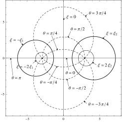
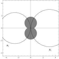
Figure 2.1: Bipolar coordinate system for $r_{1}=2.5,r_{2}=3$. The distance $\epsilon$ between disks are 2 in the left and 0.1 in the right figure; $(\xi_{1},\xi_{2})$ is $(0.99927,0.86602)$ and $(0.21021,0.17557)$ in the left and right figure, respectively. As $\epsilon$ decreases, so do $\xi_{1}$ and $\xi_{2}$ in the order of $\sqrt{\epsilon}$, see (2.7). In the left figure, solid lines are the coordinate curves of $\xi$-variable and the dotted ones are that of $\theta$. The shadow region in the right figure is $\{-\pi+\epsilon^{1/4}\leq\theta\leq\pi-\epsilon^{1/4}\}$. All points outside the shadow region have the bipolar coordinate $\theta$ close to $\pm\pi$.

Since $\partial B_{j}\mbox{ is the coordinate curve }\{\xi=(-1)^{j}\xi_{j}\}$ for $\xi_{j}$ defined as (1.13), we have

$$\xi_{j}=\sinh^{-1}\left(\frac{\alpha}{r_{j}}\right)\mbox{ and }\mathbf{c}_{j}=\alpha\bigr{(}(-1)^{j}\coth\xi_{j},0\bigr{)},\quad\mbox{for }j=1,2.$$ (2.7)

Hence $\xi_{j}={\alpha}/{r_{j}}+O(\epsilon\sqrt{\epsilon})$, $j=1,2$, and

$$\frac{\alpha}{\xi_{1}+\xi_{2}} =\frac{r_{*}^{2}}{2}+O({\epsilon}).$$ (2.8)

From (2.6), the outward unit normal $\nu$ to the circle $\xi=c$ for nonzero $c$ is

$$\nu_{\xi=c}=\frac{\nabla f_{\xi}}{|\nabla f_{\xi}|}=\mbox{sgn}(c)\left(\frac{-1-\cos\theta\cosh c}{\cosh c+\cos\theta},\ \frac{-\sin\theta\sinh c}{\cosh c+\cos\theta}\right),$$

where sgn$(c)$ takes the value of 1 or -1 as $c$ is positive or negative, respectively. We define the tangential vector $T$ as the rotation of $\nu$ by $\pi/2$-radians. One can see that

$$\nu_{\xi=c}=-\mbox{sgn}(c)\hat{\mathbf{e}}_{\xi},\ T_{\xi=c}=-\mbox{sgn}(c)\hat{\mathbf{e}}_{\theta},$$

where unit orthogonal basis vectors $\{\hat{\mathbf{e}}_{\xi},\hat{\mathbf{e}}_{\theta}\}$ are defined as

$$\hat{\mathbf{e}}_{\xi}:=\frac{\partial\mathbf{x}/\partial\xi}{|\partial\mathbf{x}/\partial\xi|}\quad\mbox{and}\quad\hat{\mathbf{e}}_{\theta}:=\frac{\partial\mathbf{x}/\partial\theta}{|\partial\mathbf{x}/\partial\theta|}.$$

It can be easily shown that the gradient of any scalar valued function $g$ is written in the following form:

$$\nabla g=\frac{\cosh\xi+\cos\theta}{\alpha}\left(\frac{\partial g}{\partial\xi}\hat{\mathbf{e}}_{\xi}+\frac{\partial g}{\partial\theta}\hat{\mathbf{e}}_{\theta}\right).$$ (2.9)

Hence the normal- and tangential derivatives of a function $u$ in bipolar coordinates are

$$\frac{\partial u}{\partial\nu}\Bigr{|}_{\xi=c} =\nabla u\cdot v_{\xi=c}=-\mbox{sgn}(c)\left(\frac{\cosh c+\cos\theta}{\alpha}\right)\frac{\partial u}{\partial\xi}\Bigr{|}_{\xi=c}$$ (2.10)

$$\frac{\partial u}{\partial T}\Bigr{|}_{\xi=c} =-\mbox{sgn}(c)\left(\frac{\cosh c+\cos\theta}{\alpha}\right)\frac{\partial u}{\partial\theta}\Bigr{|}_{\xi=c}.$$ (2.11)

The bipolar coordinate system is an orthogonal coordinate system and admits a general separation of variables solution to the harmonic function $f$ as follows:

$$f(\xi,\theta) =a_{0}+b_{0}\xi+c_{0}\theta+\sum_{n=1}^{\infty}\bigr{[}(a_{n}e^{n\xi}+b_{n}e^{-n\xi})\cos n\theta+\bigr{(}c_{n}e^{n\xi}+d_{n}e^{-n\xi})\sin n\theta\bigr{]},$$

where $a_{n}$, $b_{n}$, $c_{n}$ and $d_{n}$ are constants. Especially, the two linear functions $x$ and $y$ can be expanded as the following. For $\xi>0$, we have

$$\frac{\sinh\xi-i\sin\theta}{\cosh\xi-\cos\theta} =\frac{e^{\zeta}+e^{-\zeta}}{e^{\zeta}-e^{-\zeta}}=1+2\sum_{n=1}^{\infty}e^{-n\xi}(\cos n\theta-i\sin n\theta),$$ (2.12)

with $\zeta=\frac{\xi+i\theta}{2}$. Plugging $(\theta+\pi)$ instead of $\theta$ and using (2.3),

$$\displaystyle x =\mbox{sgn}({\xi})\alpha\bigr{[}1+2\sum_{n=1}^{\infty}(-1)^{n}e^{-n|\xi|}\cos n\theta\bigr{]},$$

$$\displaystyle y =-2\alpha\sum_{n=1}^{\infty}(-1)^{n}e^{-n|\xi|}\sin n\theta.$$

2.2 The Lerch transcendent function

The Lerch transcendent function $\Phi$ is defined as

$$\Phi(z,s,\beta):=\sum_{n=0}^{\infty}\frac{z^{n}}{(n+\beta)^{s}}\quad\mbox{ for }s\in\mathbb{C},|z|<1\mbox{ and }\beta\neq 0,-1,-2,....$$ (2.13)

The Lerch transcendent function has an integral representation

$$\Phi(z,1,\beta)=\int_{0}^{1}\frac{t^{\beta-1}}{1-zt}\ dt$$

since we have

$$\Phi(z,1,\beta) =\sum_{n=0}^{\infty}z^{n}\int_{0}^{1}t^{n+\beta-1}dt=\int_{0}^{1}t^{\beta-1}\sum_{n=0}^{\infty}\big{(}zt\big{)}^{n}dt.$$

Here, interchanging the integral and series is possible due to uniform convergence of the series for $|z|<1$. Applying the change of variables,

$$\Phi(z,1,\beta)=\int_{0}^{\infty}\frac{e^{-\beta t}}{1-ze^{-t}}\ dt.$$ (2.14)

One can easily show that

$$L(z;\beta)=-z\Phi(-z,1,\beta+1)$$

and, from (1.18),

$$P(z;\beta)=\frac{z}{1+z}-\beta z\Phi(-z,1,\beta+1).$$ (2.15)

The function $P$ is crucial to understand the blow-up feature of $\nabla u$. To understand better, let us replace the summation in $P$ by an integral in terms of the function

$$p_{\theta}(t):=\frac{1}{1+e^{-t+i\theta}}\quad\mbox{ defined for }t>0,\ \theta\in(-\pi,\pi].$$

Using (2.14), we can express $P$ as

$$P(e^{-s+i\theta};\beta)=-p_{\theta}(s)+\beta\int_{0}^{\infty}e^{-\beta t}p_{\theta}(t+s)dt,\quad s>0.$$ (2.16)

Applying the integration by parts, it becomes

$$P(e^{-s+i\theta};\beta)=\int_{0}^{\infty}e^{-\beta t}{p_{\theta}^{\prime}{}}(t+s)dt.$$ (2.17)

2.3 Properties of $P$

Recall that

$$p_{\theta}(t)=\frac{e^{t}+\cos\theta-i\sin\theta}{2(\cosh t+\cos\theta)}=\frac{1}{2}+\frac{\sinh t-i\sin\theta}{2(\cosh t+\cos\theta)},$$ (2.18)

and the derivative of $p_{\theta}$ satisfies

$$p_{\theta}^{\prime}(t)=\frac{e^{-t+i\theta}}{(1+e^{-t+i\theta})^{2}}=\frac{1+\cosh t\cos\theta+i\sinh t\sin\theta}{2(\cosh t+\cos\theta)^{2}}.$$ (2.19)

Since $\left|1+e^{-t+i\theta}\right|=\sqrt{2e^{-t}(\cosh t+\cos\theta)}$, we have

$$\displaystyle|p_{\theta}(t)| \leq\begin{cases}\displaystyle\frac{2}{\sqrt{\cosh s+\cos\theta}},\quad&\mbox{for }0<s\leq t<1\\[5.69054pt] \displaystyle 2,&\mbox{for }t\geq 1,\end{cases}$$ (2.20)

$$|p_{\theta}^{\prime}(t)| =\frac{1}{{2(\cosh t+\cos\theta)}},\quad t>0.$$ (2.21)

Lemma 2.1

Set $\beta,s,s_{1},s_{2}>0$ and $s_{1}<s_{2}$. For all $\theta\in(-\pi,\pi]$,

$$\left|P(e^{-s+i\theta};\beta)\right|\leq\frac{1}{2\beta(\cosh s+\cos\theta)},$$ (2.22)

$$\left|P(e^{-s+i\theta};\beta)\right|\leq 4+\frac{4}{\sqrt{\cosh s+\cos\theta}},$$ (2.23)

$$\left|P(e^{-s_{2}+i\theta};\beta)-P(e^{-s_{1}+i\theta};\beta)\right|\leq\frac{s_{2}-s_{1}}{\cosh s_{1}+\cos\theta}.$$ (2.24)

Proof.  If $s>1$, then we have $|P(\theta;s,\beta)|\leq 4$ from (2.20). Set $s<1$, then

$$|p_{\theta}(t)|\leq\frac{2}{\sqrt{\cosh s+\cos\theta}}\qquad\qquad\mbox{for }s\leq t<1.$$

Applying (2.16), it becomes

$$\left|P(e^{-s+i\theta};\beta)\right| \leq\frac{2}{\sqrt{\cosh s+\cos\theta}}\left(1+\beta\int_{0}^{1-s}e^{-\beta t}\ dt\right)+\beta\int_{1-s}^{\infty}e^{-\beta t}2dt$$

$$\leq\frac{4}{\sqrt{\cosh s+\cos\theta}}+2.$$

It proves (2.23). Moreover, from (2.17) and (2.21), we prove (2.22).

Let $t\geq 0$. From the mean value property,

$$p_{\theta}(t+s_{2})-p_{\theta}(t+s_{1}) =(s_{2}-s_{1})p_{\theta}^{\prime}(c)\quad\mbox{for some }c\in(t+s_{1},t+s_{2}).$$

Applying (2.21),

$$\left|p_{\theta}(t+s_{2})-p_{\theta}(t+s_{1})\right|\leq\frac{s_{2}-s_{1}}{2(\cosh s_{1}+\cos\theta)}.$$

Therefore we have

$$\left|p_{\theta}(s_{2})-p_{\theta}(s_{1})\right|\leq\frac{s_{2}-s_{1}}{2(\cosh s_{1}+\cos\theta)},$$

$$\left|\beta\int_{0}^{\infty}e^{-\beta t}p_{\theta}(t+s_{2})\ dt-\beta\int_{0}^{\infty}e^{-\beta t}p_{\theta}(t+s_{1})dt\right| \leq\beta\int_{0}^{\infty}e^{-\beta t}\frac{s_{2}-s_{1}}{2(\cosh s_{1}+\cos\theta)}dt.$$

This proves (2.24). $\Box$

Lemma 2.2

Let $\beta,\xi>0$. For all $\theta\in(-\pi,\pi]$, we have

$$\Bigr{|}(\cosh\xi+\cos\theta)\ P(e^{-\xi+i\theta};\beta)\Bigr{|}\leq\frac{e^{\xi}}{2(\beta+1)},$$ (2.25)

$$\frac{1}{4(\beta+1)}\leq\Re\{P(e^{-\xi};\beta)\}\leq\frac{1}{\beta+1},\quad\mbox{at }\theta=0.$$ (2.26)

Proof.  When $\theta=0$, from (2.19) and (2.17),

$$\frac{1}{4}\int_{0}^{\infty}e^{-(\beta+1)t}dt\leq\Re\{P(e^{-\xi};\beta)\}\leq\int_{0}^{\infty}e^{-(\beta+1)t}dt=\frac{1}{\beta+1}.$$

From (2.16) and (2.18),

$$\Re\{P(e^{-\xi+i\theta};\beta)\}=-\frac{\sinh\xi}{2(\cosh\xi+\cos\theta)}+\beta\int_{0}^{\infty}e^{-\beta t}\frac{\sinh(t+\xi)}{2(\cosh(t+\xi)+\cos\theta)}dt.$$

Hence

$$0 <(\cosh\xi+\cos\theta)\ \Re\{P(e^{-\xi+i\theta};\beta)\}+\frac{\sinh\xi}{2}=\beta\int_{0}^{\infty}e^{-\beta t}\frac{(\cosh\xi+\cos\theta)\sinh(t+\xi)}{2(\cosh(t+\xi)+\cos\theta)}dt$$

$$\leq\beta\int_{0}^{\infty}e^{-\beta t}\frac{(\cosh\xi+1)\sinh(t+\xi)}{2(\cosh(t+\xi)+1)}\ dt=(\cosh\xi+1)\ \Re\{P(e^{-\xi};\beta)\}+\frac{\sinh\xi}{2}.$$

$\Box$

2.4 Summation formula

In this section we prove a lemma which is essential to prove the main results in this paper.

Lemma 2.3

Fix a $a_{0}>0$. For $a<a_{0}$, $0<\tau<1$ and $\theta\in(-\pi,\pi]$, we have

$$\left|a_{0}\sum_{m=1}^{\infty}\tau^{m-1}\frac{e^{-ma_{0}+a+i\theta}}{(1+e^{-ma_{0}+a+i\theta})^{2}}-P(e^{-(a_{0}-a)+i\theta};-(\ln\tau)/a_{0})\right|\leq\frac{4a_{0}}{\cosh(a_{0}-a)+\cos\theta}.$$

Proof.  Fix a $\theta$. Thanks to (2.19),

$$a_{0}\sum_{m=1}^{\infty}\tau^{m-1}\frac{e^{-ma_{0}+a+i\theta}}{(1+e^{-ma_{0}+a+i\theta})^{2}}=a_{0}\sum_{m=0}^{\infty}\tau^{m}p_{\theta}^{\prime}(ma_{0}+s_{0}),\quad s_{0}=a_{0}-a>0.$$ (2.27)

To rewrite the right-hand side of (2.27), we consider $f(t):=\tau^{t}p_{\theta}^{\prime}(a_{0}t+s_{0})$. From (2.21) and the fact that $\tau\in(0,1)$,

$$\left|\tau^{t}p_{\theta}^{\prime}(a_{0}t+s_{0})\right|\leq\frac{1}{2(\cosh s_{0}+\cos\theta)},\quad t\geq 0,$$ (2.28)

and the derivative of $f$ is as follows:

$$\frac{d}{dt}\Bigr{(}\tau^{t}p_{\theta}^{\prime}(a_{0}t+s_{0})\Bigr{)}=\tau^{t}\Bigr{(}(\ln\tau)p_{\theta}^{\prime}(a_{0}t+s_{0})+sp_{\theta}^{\prime\prime}(a_{0}t+s_{0})\Bigr{)}.$$ (2.29)

Note that, from (2.19), the real and imaginary part of $e^{2(a_{0}t+s_{0})}\Bigr{(}(\ln\tau)p_{\theta}^{\prime}(a_{0}t+s_{0})+a_{0}p_{\theta}^{\prime\prime}(a_{0}t+s_{0})\Bigr{)}$ are quadratic polynomials of $e^{a_{0}t+s_{0}}$. Hence the real and imaginary part of $\frac{d}{dt}\Bigr{(}\tau^{t}p_{\theta}^{\prime}(a_{0}t+s_{0})\Bigr{)}$ changes the sign at most 4 times on $(0,\infty)$. Therefore, from (2.21),

$$\left|a_{0}\sum_{m=0}^{\infty}\tau^{m}p_{\theta}^{\prime}(ma_{0}+s_{0})-a_{0}\int_{0}^{\infty}\tau^{t}p_{\theta}^{\prime}(a_{0}t+s_{0})dt\right|\leq 8\sup_{t\geq 0}|p_{\theta}^{\prime}(t)|\leq\frac{4a_{0}}{{\cosh s_{0}+\cos\theta}}.$$

By a change of variables, we get

$$\displaystyle a_{0}\int_{0}^{\infty}\tau^{t}p_{\theta}^{\prime}(a_{0}t+s_{0})dt =\int_{0}^{\infty}e^{-bt}p_{\theta}^{\prime}(t+s_{0})dt=-p_{\theta}(s_{0})+b\int_{0}^{\infty}e^{-bt}p_{\theta}(t+s_{0})\ dt$$

with $b=\frac{-\log\tau}{a_{0}}$. This proves the lemma. $\Box$

3 Expansion of $u$ in terms of the bipolar system

From (1.5), we only need to consider linear functions for $H$. We can also assume $B_{1}$ and $B_{2}$ satisfy (2.2) without loss of generality. Define the bipolar system $(\xi,\theta)$ and $\xi_{j}$, $j=1,2$, as in section 2.1. So $\xi=-\xi_{1}$ and $\xi=\xi_{2}$ represents $\partial B_{1}$ and $\partial B_{2}$, respectively. Set

$$\xi_{M}:=\max(\xi_{1},\xi_{2})\mbox{ and }\xi_{s}:=\min(\xi_{1},\xi_{2}),$$

then

$$\begin{cases}-\xi-2\xi_{1},\xi-2\xi_{2}\in(-2\xi_{M}-\xi_{s},-\xi_{s}),\ &\mathbf{x}\in\mathbb{R}^{2}\setminus\overline{B_{1}\cup B_{2}}\\ \xi\in(-\infty,-\xi_{1}),&\mathbf{x}\in B_{1}\\ \xi\in(\xi_{2},\infty),&\mathbf{x}\in B_{2}.\end{cases}$$ (3.1)

Lemma 3.1

Define a complex valued function

$$U(x,y):=C+\begin{cases}\displaystyle\sum_{n=1}^{\infty}\left(A_{n}e^{n(\xi+i\theta)}+B_{n}e^{-n(\xi+i\theta)}\right),\quad&x\in\mathbb{R}^{2}\setminus(B_{1}\cup B_{2})\\ \displaystyle\sum_{n=1}^{\infty}\left(A_{n}e^{n(\xi+i\theta)}+B_{n}e^{n(2\xi_{1}+\xi-i\theta)}\right),&x\in B_{1}\\ \displaystyle\sum_{n=1}^{\infty}\left(A_{n}e^{n(2\xi_{2}-\xi+i\theta)}+B_{n}e^{-n(\xi+i\theta)}\right),&x\in B_{2}\end{cases}$$ (3.2)

where $C=-\sum_{n=1}^{\infty}(A_{n}+B_{n})\cos n\pi$ and

$$\displaystyle A_{n} =\frac{2\alpha(-1)^{n}}{\tau^{-1}e^{2n(\xi_{1}+\xi_{2})}-1}\left(-\frac{1}{\tau_{1}}e^{2n\xi_{1}}-1\right),\ \displaystyle B_{n}=\frac{2\alpha(-1)^{n}}{\tau^{-1}e^{2n(\xi_{1}+\xi_{2})}-1}\left(1+\frac{1}{\tau_{2}}e^{2n\xi_{2}}\right).$$

Then $(x+\Re\{U\})$ is the solution to (1.2) for $H(x,y)=x$, and $(y+\Im\{U\})$ is the solution for $H(x,y)=y$ with $1/k_{j}$ in the place of $k_{j}$, $j=1,2$.

We prove the lemma after the following one.

Lemma 3.2

Suppose $\tau\geq 0.5$. There is a constant $C$ depending only on $r_{1},r_{2}$ such that

$$\left|\frac{\partial U}{\partial\xi}(\mathbf{x})-r_{*}^{2}\frac{\partial}{\partial\xi}q(\mathbf{x};\beta,\tau_{1},\tau_{2})\right|\leq\frac{C}{\cosh\xi_{s}+\cos\theta},\quad\mathbf{x}\in\mathbb{R}^{2},$$

where $q$ is defined as (1.14). We have the same equation for the partial derivative in $\theta$ variable.

Proof.  Note that $A_{n}$ and $B_{n}$ can be represented as

$$A_{n} =2\alpha(-1)^{n}\sum_{m=1}^{\infty}\tau^{m}\left(-\frac{1}{\tau_{1}}\ e^{2n\xi_{1}}-1\right)e^{-2nm(\xi_{1}+\xi_{2})},$$

$$B_{n} =2\alpha(-1)^{n}\sum_{m=1}^{\infty}\tau^{m}\left(1+\frac{1}{\tau_{2}}\ e^{2n\xi_{2}}\right)e^{-2nm(\xi_{1}+\xi_{2})}.$$

Firstly, set $-\xi_{1}\leq\xi\leq\xi_{2}$. By interchanging the order of summation, which is possible due to the absolute convergence, we have

$$\sum_{n=1}^{\infty}n\left(A_{n}e^{n(\xi+i\theta)}-B_{n}e^{-n(\xi+i\theta)}\right)$$

$$=-2\alpha\sum_{m=1}^{\infty}\tau^{m}\Bigg{[}\ \frac{1}{\tau_{1}}\displaystyle\sum_{n=1}^{\infty}n\left(-e^{-2m(\xi_{1}+\xi_{2})+2\xi_{1}+\xi+i\theta}\right)^{n}+\sum_{n=1}^{\infty}n\left(-e^{-2m(\xi_{1}+\xi_{2})+\xi+i\theta}\right)^{n}$$

$$\quad\quad\displaystyle+\frac{1}{\tau_{2}}\sum_{n=1}^{\infty}n\left(-e^{-2m(\xi_{1}+\xi_{2})+2\xi_{2}-\xi-i\theta}\right)^{n}+\sum_{n=1}^{\infty}n\left(-e^{-2m(\xi_{1}+\xi_{2})-\xi-i\theta}\right)^{n}\Bigg{]}.$$ (3.3)

Using the following formula $\sum_{n=1}^{\infty}nz^{n}=\frac{z}{(1-z)^{2}},\mbox{ for }|z|<1,\ z\in\mathbb{C},$ we have

$$\sum_{n=1}^{\infty}n\left(A_{n}e^{n(\xi+i\theta)}-B_{n}e^{-n(\xi+i\theta)}\right)$$

$$=2\alpha\tau\sum_{m=1}^{\infty}\tau^{m-1}\Bigg{[}\frac{1}{\tau_{1}}\frac{e^{-2m(\xi_{1}+\xi_{2})+2\xi_{1}+\xi+i\theta}}{(1+e^{-2m(\xi_{1}+\xi_{2})+2\xi_{1}+\xi+i\theta})^{2}}+\frac{e^{-2m(\xi_{1}+\xi_{2})+\xi+i\theta}}{(1+e^{-2m(\xi_{1}+\xi_{2})+\xi+i\theta})^{2}}$$

$$\quad\quad+\frac{1}{\tau_{2}}\frac{e^{-2m(\xi_{1}+\xi_{2})+2\xi_{2}-\xi-i\theta}}{(1+e^{-2m(\xi_{1}+\xi_{2})+2\xi_{2}-\xi-i\theta})^{2}}+\frac{e^{-2m(\xi_{1}+\xi_{2})-\xi-i\theta}}{(1+e^{-2m(\xi_{1}+\xi_{2})-\xi-i\theta})^{2}}\Bigg{]}.$$ (3.4)

We apply Lemma 2.3 to this series with $a=2(\xi_{1}+\xi_{2})$. From (3.3), (3.4), Lemma 2.3, and Lemma 2.1,

$$\sum_{n=1}^{\infty}n\left(A_{n}e^{n(\xi+i\theta)}-B_{n}e^{-n(\xi+i\theta)}\right)$$

$$=\frac{{r_{*}^{2}}}{2}\Bigg{[}\tau_{2}P(e^{-2\xi_{2}+\xi+i\theta};b)+\tau P(e^{-2(\xi_{1}+\xi_{2})+\xi+i\theta};b)+\tau_{1}P(e^{-2\xi_{1}-\xi-i\theta};b)$$

$$\qquad\qquad+\tau P(e^{-2(\xi_{1}+\xi_{2})-\xi-i\theta};b)\Bigg{]}+\frac{r_{*}^{2}(\tau_{1}+\tau_{2}+2\tau_{1}\tau_{2})}{2}\frac{O(\sqrt{\epsilon})}{\cosh\xi_{s}+\cos\theta},$$

where

$$b=\frac{-\ln\tau}{2(\xi_{1}+\xi_{2})}.$$

Note that $b=\beta+O(\sqrt{\epsilon})$ where $\beta$ is defined as (1.15). Since $b,\beta>0$, applying the mean value property for a fixed $t>0$, we have

$$be^{-bt}=\beta e^{-\beta t}+(b-\beta)(1-st)e^{-st},\quad\mbox{for a }s\in(\min(b,\beta),\ \max(b,\beta)).$$ (3.5)

Hence

$$be^{-bt}-\beta e^{-\beta t}=\begin{cases}(b-\beta)O(1),\quad&\mbox{for }t>0,\\ (b-\beta)O(t)e^{-\min(b,\beta)t},\quad&\mbox{for }t\geq 1.\end{cases}$$ (3.6)

Therefore, using (2.20) as well,

$$\left|b\int_{0}^{\infty}e^{-bt}p_{\theta}(t+\xi_{s})dt-\beta\int_{0}^{\infty}e^{-\beta t}p_{\theta}(t+\xi_{s})dt\right|$$

$$\leq|b-\beta|\int_{0}^{1}O(1)\frac{1}{\sqrt{\cosh\xi_{s}+\cos\theta}}\ dt+|b-\beta|\int_{1}^{\infty}e^{-\min{(b,\beta)}t}O(t)dt$$

$$\displaystyle\leq C\sqrt{\epsilon}\frac{1}{\cosh\xi_{s}+\cos\theta}+O(\sqrt{\epsilon}).$$

Here the remainder term $O(\sqrt{\epsilon})$ is uniform with respect to $k_{1},k_{2},{\xi}$ and $\theta$. Therefore we can replace $b$ by $\beta$. Using (2.8), we prove the lemma for $-\xi_{1}\leq\xi\leq\xi_{2}$.

Similarly, for $\xi\leq-\xi_{1}$, we can derive that

$$\displaystyle\sum_{n=1}^{\infty}n\left(A_{n}e^{n(\xi+i\theta)}\pm B_{n}e^{2n\xi_{1}}e^{n(\xi-i\theta)}\right)$$

$$=\frac{{r_{*}^{2}}}{2}\Bigg{[}(\tau_{2}+\tau)P(e^{\xi+i\theta-2\xi_{2}};\beta)\mp(\tau_{1}+\tau)P(e^{\xi-i\theta};\beta)\Bigg{]}+\frac{O(\sqrt{\epsilon})}{\cosh\xi_{s}+\cos\theta},$$

and, for $\xi\geq\xi_{2}$,

$$\displaystyle\sum_{n=1}^{\infty}n\left(\mp A_{n}e^{2\xi_{2}}e^{-n(\xi-i\theta)}-B_{n}e^{-n(\xi+i\theta)}\right)$$

$$=\frac{{r_{*}^{2}}}{2}\Bigg{[}\mp(\tau_{2}+\tau)P(e^{-\xi+i\theta};\beta)+(\tau_{1}+\tau)P(e^{-\xi-i\theta-2\xi_{1}};\beta)\Bigg{]}+\frac{O(\sqrt{\epsilon})}{\cosh\xi_{s}+\cos\theta}.$$

This proves the lemma for $\xi\leq-\xi_{1}$ and for $\xi\geq\xi_{2}$. $\Box$

Proof of Lemma 3.1 It can be easily shown that the function $u$ defined as (3.2) satisfies the transmission condition of (1.3). Hence it is only need to show that there is a positive constant $M$ such that

$$\limsup_{|\mathbf{x}|\rightarrow\infty}|\mathbf{x}||(u-H)(\mathbf{x})|\leq M.$$ (3.7)

From (2.5), it is enough to show that

$$\limsup_{(\xi,\theta)\rightarrow(0,\pi)}\frac{|(u-H)(\mathbf{x})|}{\sqrt{\cosh\xi+\cos\theta}}\leq M$$

when the distance $\epsilon$ is fixed.

Plugging $\xi=0$ and $\theta=\pi$ into (3.3), it becomes

$$\sum_{n=1}^{\infty}\bigr{[}(A_{n}+B_{n})\cos n\pi\bigr{]} =2\alpha\tau\sum_{m=1}^{\infty}\tau^{m-1}\Bigg{[}\frac{1}{\tau_{1}}\frac{-e^{-2m(\xi_{1}+\xi_{2})+2\xi_{2}}}{1-e^{-2m(\xi_{1}+\xi_{2})+2\xi_{2}}}+\frac{-e^{-2m(\xi_{1}+\xi_{2})}}{1-e^{-2m(\xi_{1}+\xi_{2})}}$$

$$\qquad\qquad\quad\quad-\frac{1}{\tau_{2}}\frac{-e^{-2m(\xi_{1}+\xi_{2})+2\xi_{1}}}{1-e^{-2m(\xi_{1}+\xi_{2})+2\xi_{1}}}-\frac{-e^{-2m(\xi_{1}+\xi_{2})}}{1-e^{-2m(\xi_{1}+\xi_{2})}}\Bigg{]}.$$

Note that for $\tilde{\xi}=0,2\xi_{1},2\xi_{2}$ and $|\xi|\leq\xi_{s}$. Hence we have

$$\left|\frac{e^{-2m(\xi_{1}+\xi_{2})+\tilde{\xi}+\xi+i\theta}}{1+e^{-2m(\xi_{1}+\xi_{2})+\tilde{\xi}+\xi+i\theta}}-\frac{-e^{-2m(\xi_{1}+\xi_{2})+\tilde{\xi}}}{1-e^{-2m(\xi_{1}+\xi_{2})+\tilde{\xi}}}\right| =\left|\frac{(e^{\xi+i\theta}+1)e^{-2m(\xi_{1}+\xi_{2})+\tilde{\xi}}}{(1+e^{-2m(\xi_{1}+\xi_{2})+\tilde{\xi}+\xi+i\theta})(1-e^{-2m(\xi_{1}+\xi_{2})+\tilde{\xi}})}\right|$$

$$\leq\frac{e^{-2m(\xi_{1}+\xi_{2})+\tilde{\xi}+\xi_{s}}}{(1-e^{-2m(\xi_{1}+\xi_{2})+\tilde{\xi}+\xi_{s}})^{2}}|e^{\xi+i\theta}+1|.$$

Let us define a constant

$$S :=2\alpha\tau\sum_{m=1}^{\infty}\tau^{m-1}\Bigg{[}\left(\frac{1}{\tau_{1}}\right)\frac{e^{-2m(\xi_{1}+\xi_{2})+2\xi_{2}+\xi_{s}}}{(1-e^{-2m(\xi_{1}+\xi_{2})+2\xi_{2}+\xi_{s}})^{2}}+\frac{e^{-2m(\xi_{1}+\xi_{2})+\xi_{s}}}{(1-e^{-2m(\xi_{1}+\xi_{2})+\xi_{s}})^{2}}$$

$$\qquad\qquad\quad\quad+\left(\frac{1}{\tau_{2}}\right)\frac{e^{-2m(\xi_{1}+\xi_{2})+2\xi_{1}+\xi_{s}}}{(1-e^{-2m(\xi_{1}+\xi_{2})+2\xi_{1}+\xi_{s}})^{2}}+\frac{e^{-2m(\xi_{1}+\xi_{2})+\xi_{s}}}{(1-e^{2m(\xi_{1}+\xi_{2})+\xi_{s}})^{2}}\Bigg{]}.$$

Applying the same procedure as in the proof of Lemma 3.2 , we have

$$|(u-H)(\mathbf{x})| =\left|\sum_{n=1}^{\infty}\bigr{[}(A_{n}e^{n\xi}+B_{n}e^{-n\xi})\cos n\theta-(A_{n}+B_{n})\cos n\pi\bigr{]}\right|$$

$$\leq S|e^{\xi+i\theta}+1|.$$

Hence $\left|(u-H)(\mathbf{x})\right|\leq C|\xi+i(\theta-\pi)|,\mbox{ as }(\xi,\theta)\rightarrow(0,\pi),$ with a constant $C$ independent of $\xi$ and $\theta$. $\Box$

Lemma 3.3

The singular function $q$ in (1.14) satisfies

$$q(\mathbf{x};\beta,\tau_{1},\tau_{2})-C_{q}=O(|\mathbf{x}|^{-1}),\quad\mbox{as }|\mathbf{x}|\rightarrow\infty,$$

Where $C_{q}$ is a constant defined as $C_{q}=\frac{1}{2}\Bigr{\{}(\tau_{1}+\tau)L(-e^{-2\xi_{1}};\beta)-(\tau_{2}+\tau)L(-e^{-2\xi_{2}};\beta)\Bigr{\}}.$

Proof.  From the definition of $L$, we have

$$\displaystyle\left|L(e^{-(\xi+i\theta)-2\xi_{1}};\beta)-L(e^{-2\xi_{1}};\beta)\right|\displaystyle \leq\int_{0}^{1}t^{\beta}\left|\frac{e^{-(\xi+i\theta)-2\xi_{1}}}{1+te^{-(\xi+i\theta)-2\xi_{1}}}-\frac{-e^{-2\xi_{1}}}{1-te^{-2\xi_{1}}}\right|dt$$

$$=\int_{0}^{1}t^{\beta}\left|\frac{(e^{-(\xi+i\theta)}+1)te^{-2\xi_{1}}}{(1+te^{-(\xi+i\theta)-2\xi_{1}})(1-te^{-2\xi_{1}})}\right|dt$$

$$=\left|e^{-(\xi+i\theta)}+1\right|\int_{0}^{1}t^{\beta}\left|\frac{te^{-2\xi_{1}}}{(1-te^{-2\xi_{1}})^{2}}\right|dt$$

$$\leq C|\xi+i(\theta-\pi)|,\quad\mbox{as }(\xi,\theta)\rightarrow(0,\pi),$$

where a constant $C$ is independent of $\xi$ and $\theta$. Therefore, we have

$$L(e^{-(\xi+i\theta)-2\xi_{1}};\beta)-L(e^{-2\xi_{1}};\beta)=O(|\mathbf{x}|^{-1}),\quad\mbox{as }|\mathbf{x}|\rightarrow\infty.$$

Similarly, we prove the deacay property of $L(e^{(\xi+i\theta)-2\xi_{2}};\beta)-L(e^{-2\xi_{2}};\beta)$. $\Box$

4 Asymptotic Estimates for $\nabla u$

4.1 Estimates of the gradient of the singular function $q$

The main term of $u$ in both Theorem 1.1 and Theorem 1.2 is expressed in terms of $q(\mathbf{x};\beta,\tau_{1},\tau_{2})$ with positive $\tau_{1}$ and $\tau_{2}$. We assume that $\tau_{1}$ and $\tau_{2}$ are positive in this section.

For notational sake, the normal- and the tangential derivatives at $(c,\theta)$ mean (2.10) and (2.11), respectively, on the coordinate level curve $\{\xi=c\}$. From (1.14) and (1.18), the derivative of $q(\mathbf{x};\beta,\tau_{1},\tau_{2})$ satisfies

$$\frac{\partial q}{\partial\xi}=\frac{1}{2}\begin{cases}\displaystyle(\tau_{1}+\tau)P\bigr{(}e^{-(\xi+i\theta)-2\xi_{1}};\beta\bigr{)}+(\tau_{2}+\tau)P\bigr{(}e^{(\xi+i\theta)-2\xi_{2}};\beta\bigr{)}\ &\mbox{in }\mathbb{R}^{2}\setminus\overline{(B_{1}\cup B_{2})},\\[2.84526pt] \displaystyle-(\tau_{1}+\tau)P\big{(}e^{\xi-i\theta};\beta\big{)}+(\tau_{2}+\tau)P\big{(}e^{\xi+i\theta-2\xi_{2}};\beta\big{)}\quad&\mbox{in }B_{1},\\[2.84526pt] \displaystyle(\tau_{1}+\tau)P\big{(}e^{-\xi-i\theta-2\xi_{1}};\beta\big{)}-(\tau_{2}+\tau)P\big{(}e^{-\xi+i\theta};\beta\big{)}\quad&\mbox{in }B_{2},\\[5.69054pt] \end{cases}$$ (4.1)

$$\frac{\partial q}{\partial\theta}=\frac{i}{2}\begin{cases}\displaystyle(\tau_{1}+\tau)P\bigr{(}e^{-(\xi+i\theta)-2\xi_{1}};\beta\bigr{)}+(\tau_{2}+\tau)P\bigr{(}e^{(\xi+i\theta)-2\xi_{2}};\beta\bigr{)}\ &\mbox{in }\mathbb{R}^{2}\setminus\overline{(B_{1}\cup B_{2})},\\[2.84526pt] \displaystyle(\tau_{1}+\tau)P\big{(}e^{\xi-i\theta};\beta\big{)}+(\tau_{2}+\tau)P\big{(}e^{\xi+i\theta-2\xi_{2}};\beta\big{)}\quad&\mbox{in }B_{1},\\[2.84526pt] \displaystyle(\tau_{1}+\tau)P\big{(}e^{-\xi-i\theta-2\xi_{1}};\beta\big{)}+(\tau_{2}+\tau)P\big{(}e^{-\xi+i\theta};\beta\big{)}\quad&\mbox{in }B_{2},\end{cases}$$

where $P$ is defined as (1.18). From (2.10), (2.11), (2.23) and (2.8)

$$(\nabla q\cdot\hat{\mathbf{e}}_{\xi})\bigr{|}_{\xi=c} =\frac{\cosh c+\cos\theta}{r_{*}\sqrt{\epsilon}}\frac{\partial q}{\partial\xi}\Bigr{|}_{\xi=c}+O(1),$$ (4.2)

$$(\nabla q\cdot\hat{\mathbf{e}}_{\theta})\bigr{|}_{\xi=c} =\frac{\cosh c+\cos\theta}{r_{*}\sqrt{\epsilon}}\frac{\partial q}{\partial\theta}\Bigr{|}_{\xi=c}+O(1).$$ (4.3)

Lemma 4.1

There is a constant $C$ independent of $\epsilon$, $k_{1}$, and $k_{2}$ such that

$$\|\nabla q\|_{L^{\infty}(\mathbb{R}^{2})}\leq C\mbox{ if }\tau<\frac{1}{2}.$$

Proof.  Applying (3.1) to (2.23) for $\mathbf{x}\in B_{1}\cup B_{2}$ and (2.25) for $\mathbf{x}\in\mathbb{R}^{2}\setminus\overline{B_{1}\cup B_{2}}$, we can prove than there is a $C$ independent of $\epsilon$, $k_{1}$ and $k_{2}$ such that

$$\left|(\nabla q\cdot\hat{\mathbf{e}}_{\xi})\right|,\left|(\nabla q\cdot\hat{\mathbf{e}}_{\theta})\right|\leq C\frac{1}{-\ln\tau},$$ (4.4)

for $c\neq-\xi_{1},\xi_{2}$. At $c=(-1)^{j}\xi_{j}$, $j=1,2$, (4.4) is satisfied for either outward or inward derivatives. $\Box$

Proposition 4.2

Suppose $\tau_{1},\tau_{2}>0$. The tangential derivative of $\Re\{q(\mathbf{x};\beta,\tau_{1},\tau_{2})\}$ is remain bounded regardless of $\epsilon$ for all $\mathbf{x}\in\mathbb{R}^{2}$. The normal derivative of $\Re\{q(\mathbf{x};\beta,\tau_{1},\tau_{2})\}$ is bounded in $B_{1}\cup B_{2}$. For $\mathbf{x}\notin\overline{B_{1}\cup B_{2}}$,

$$\frac{\partial\Re\{q\}}{\partial\nu}\bigg{|}_{\xi=c}=-\mbox{sgn}(c)\left(\tau_{1}+\tau_{2}+2\tau\right)\frac{\cosh\xi_{s}+\cos\theta}{2r_{*}\sqrt{\epsilon}}\Re\left\{P\bigr{(}e^{-(\xi_{s}+i\theta)};\beta\bigr{)}\right\}+O(1).$$ (4.5)

Proof.  From the definition of $P$,

$$P(\overline{z};\beta)=\overline{P(z;\beta)},\quad\mbox{for all }z\in\mathbb{C},|z|<1.$$ (4.6)

Hence

$$\Re\{P(\overline{z})\}=\Re\{P(z)\}\mbox{ and }\Im\{P(\overline{z})\}=-\Im\{P(z)\}.$$ (4.7)

From (4.1), (4.7), (2.24) and (4.2), we have

$$\displaystyle\frac{\partial\Re\{q\}}{\partial\nu}\bigg{|}_{\xi=c}=-\mbox{sgn}(c)\begin{cases}\displaystyle\frac{\cosh\xi_{s}+\cos\theta}{2r_{*}\sqrt{\epsilon}}\left(\tau_{1}+\tau_{2}+2\tau\right)\Re\left\{P\bigr{(}e^{-\xi_{s}+i\theta};\beta\bigr{)}\right\}+O(1),\quad&\mathbf{x}\in\mathbb{R}^{2}\setminus\overline{B_{1}\cup B_{2}}\\[5.69054pt] \displaystyle\frac{\cosh\xi+\cos\theta}{2r_{*}\sqrt{\epsilon}}\left(\tau_{2}-\tau_{1}\right)\Re\left\{P\bigr{(}e^{\xi+i\theta};\beta\bigr{)}\right\}+O(1),\quad&\mathbf{x}\in B_{1}\\[5.69054pt] \displaystyle\frac{\cosh\xi+\cos\theta}{2r_{*}\sqrt{\epsilon}}\left(\tau_{1}-\tau_{2}\right)\Re\left\{P\bigr{(}e^{-\xi+i\theta};\beta\bigr{)}\right\}+O(1),\quad&\mathbf{x}\in B_{2},\end{cases}$$

$$\displaystyle\frac{\partial\Re\{q\}}{\partial T}\bigg{|}_{\xi=c}=-\mbox{sgn}(c)\frac{\cosh c+\cos\theta}{2r_{*}\sqrt{\epsilon}}\left(\tau_{1}-\tau_{2}\right)\Re\left\{P\bigr{(}e^{-\max(\xi_{s},|c|)-i\theta};\beta\bigr{)}\right\}+O,\quad\mathbf{x}\in\mathbb{R}^{2}.$$

Let us prove the boundedness part in the corollary. From (2.22), we have

$$\left|\frac{\partial}{\partial\nu}\Re\{q(\mathbf{x};\beta,\tau_{1},\tau_{2})\}\Bigr{|}^{-}_{\partial B_{j}}\right|\leq C|\tau_{1}-\tau_{2}|\frac{1}{\sqrt{\epsilon}}\frac{1}{2\beta}O(1)+O(1).$$

Since $|t-1|\leq-\log t\mbox{ for all }0<t<1$,

$$\frac{\left|\tau_{1}-\tau_{2}\right|}{-\log\tau}\leq\frac{\left|\tau_{1}-1\right|+\left|1-\tau_{|}\right|}{-\log\tau_{1}-\log\tau_{2}}\leq 2.$$

Hence the normal derivative inside $B_{1}$ and $B_{2}$ is bounded. Similarly, we prove the tangential derivative is bounded. $\Box$

Following the proof of Proposition 4.2, it can be easily shown the following.

Proposition 4.3

Suppose $\tau_{1},\tau_{2}>0$. The normal derivative of $\Im\{q(\mathbf{x};\beta,\tau_{1},\tau_{2})\}$ is remain bounded regardless of $\epsilon$ for $\mathbf{x}\in\mathbb{R}^{2}\setminus\overline{B_{1}\cup B_{2}}$. For $\mathbf{x}\in B_{1}\cup B_{2}$,

$$\displaystyle\frac{\partial\Im\{q\}}{\partial\nu}\bigg{|}_{\xi=c}=\frac{\cosh c+\cos\theta}{2r_{*}\sqrt{\epsilon}}\left(\tau_{1}+\tau_{2}+2\tau\right)\Re\left\{P\bigr{(}e^{-|c|+i\theta};\beta\bigr{)}\right\}+O(1).$$

The tangential derivative satisfies

$$\frac{\partial\Im\{q\}}{\partial T}\bigg{|}_{\xi=c}=-\mbox{sgn}(c)\left(\tau_{1}+\tau_{2}+2\tau\right)\frac{\cosh c+\cos\theta}{2r_{*}\sqrt{\epsilon}}\Re\left\{P\bigr{(}e^{-\max(\xi_{s},|c|)-i\theta)};\beta\bigr{)}\right\}+O(1),\quad\mathbf{x}\in\mathbb{R}^{2}.$$ (4.8)

Corollary 4.4

Suppose $k_{1},k_{2}>1$ From Theorem 1.1, Theorem 1.2, Proposition 4.2 and Proposition 4.3, we have

$$\bigr{|}\nabla(u-H)\bigr{|}^{+}(\mathbf{x})=|c_{\mathbf{n}}|\left(|\tau_{1}|+|\tau_{2}|+2\tau\right)\frac{\cosh\xi_{j}+\cos\theta}{2r_{*}\sqrt{\epsilon}}\left|\Re\{P\bigr{(}e^{-(\xi_{j}+i\theta)};\beta\bigr{)}\}\right|+O(1)$$

on $\partial B_{j}$, $j=1,2$. Especially at $\mathbf{x}_{j}$, which is the point on $\partial B_{j}$ closest to the other disk, we have $\theta=0$ and

$$\bigr{|}\nabla(u-H)\bigr{|}^{+}(\mathbf{x}_{j})=|c_{\mathbf{n}}|\left(|\tau_{1}|+|\tau_{2}|+2\tau\right)\frac{\cosh\xi_{j}+1}{2r_{*}\sqrt{\epsilon}}\left|\Re\{P\bigr{(}e^{-\xi_{j}};\beta\bigr{)}\}\right|+O(1).$$

The above asymptotic equations are still valid for $0<k_{1},k_{2}<1$ if $\mathbf{n}$ is replaced by $\mathbf{t}$.

Remark 4.5

Applying Lemma 2.2, it follows that there is a constant $C_{1}$ and $C_{2}$ such that

$$\left|\nabla u\right|_{+}(\mathbf{x}_{j}) \geq\frac{C_{1}r_{*}(\nabla H(\mathbf{p})\cdot\mathbf{n})}{\sqrt{\epsilon}(\beta+1)},\quad j=1,2,$$ (4.9)

$$\left\|\nabla u\right\|_{L^{\infty}(\partial B_{j})} \leq\frac{C_{2}r_{*}(\nabla H(\mathbf{p})\cdot\mathbf{n})}{\sqrt{\epsilon}(\beta+1)},$$ (4.10)

where $\mathbf{p}$ is the middle point of the shortest line segment connecting $\partial B_{1}$ and $\partial B_{2}$. Since $\beta=\frac{r_{*}}{4\sqrt{\epsilon}}(1-\tau+O((1-\tau)^{2})$,

$$\frac{r_{*}}{\sqrt{\epsilon}(\beta+1)}\approx\frac{4}{1-\tau+\frac{4}{r_{*}}\sqrt{\epsilon}}.$$

Recall that ${r_{*}}/\mbox{max}(r_{1},r_{2})\leq{1}/{r_{*}}\leq{r_{*}}/{\mbox{min}(r_{1},r_{2})}.$ Hence (4.9) and (4.10) are in accordance with the upper and lower bounds (1.6) and (1.7).

4.2 Extreme cases for $\beta$

In this section we let us consider the case when $\beta$ is extremely small or large. Recall that $\beta$ in (1.15) can be an arbitrary positive number even when $\ln\tau$ is very small because the denominator is small parameter. For example, $\beta=\frac{r_{*}}{4\sqrt{\epsilon}}(1-\tau+O((1-\tau)^{2})\approx{\epsilon}^{1/4}$ if $k_{j}\approx\epsilon^{-3/4}$, and $\beta\approx\epsilon^{-1/4}$ if $k_{j}\approx\epsilon^{-1/4}$.

From the definition $P$ in (2.15), it can be written as

$$P(z;\beta)=-\frac{1}{z+1}+\beta\Phi(-z,1,\beta).$$

Set $|z|<1$, namely, $z=-e^{-\xi+i\theta}$ with $\xi>0$. For $\beta\ll 1$,

$$\displaystyle\Phi(z,1,\beta) =\frac{1}{\beta}+\sum_{k=0}^{\infty}\frac{z^{k}}{k}-\beta\sum_{k=1}^{\infty}\frac{z^{k}}{k^{2}(1+\frac{\beta}{k})}=\frac{1}{\beta}-\log(1-z)+O(\beta)$$ (4.11)

and

$$\Re\{\Phi(z,1,\beta)\}=\frac{1}{\beta}-\ln\sqrt{2e^{-\xi}(\cosh\xi+\cos\theta)}+O(\beta).$$

If $\beta\gg 1$, applying the integration by parts twice on (2.14), we have

$$\Phi(z,1,\beta)=\frac{1}{\beta}\frac{1}{1-z}+\frac{1}{\beta^{2}}\frac{-z}{(1-z)^{2}}+\frac{1}{\beta^{3}}\frac{r(z,\beta)}{(\cosh\xi+\cos\theta)^{\frac{3}{2}}},$$ (4.12)

with $|r(z,\beta)|\leq 32.$ It is worth to mention that there are more complete results on the asymptotic expansions of $\Phi(z,s,\beta)$ for large and small $\beta$ done by Ferreira and Lopéz [11].

Applying the asymptotic of the Lerch transcendent in (4.11) and (4.12), we have

$$\Re\{P(e^{-\xi_{j}-i\theta};\beta)\} =\frac{1}{2}-\frac{\sinh\xi_{j}}{2(\cosh\xi_{j}+\cos\theta)}-\beta\ln|1+e^{-\xi_{j}-i\theta}|+O(\sqrt{\epsilon})$$

$$=\frac{1}{2}\Bigr{(}1-\beta\ln[2(\cosh\xi_{j}+\cos\theta)]\Bigr{)}+\frac{O(\sqrt{\epsilon})}{\cosh\xi_{j}+\cos\theta},\quad\mbox{for }\beta=O(\epsilon^{1/4}),$$ (4.13)

and

$$\Re\{P(e^{-\xi_{j}-i\theta};\beta)\} =\frac{1}{\beta}\frac{e^{-\xi_{j}-i\theta}}{(e^{-\xi_{j}-i\theta}+1)^{2}}+\frac{O(\sqrt{\epsilon})}{(\cosh\xi_{j}+\cos\theta)^{\frac{3}{2}}}$$

$$=\frac{1}{\beta}\frac{1+\cosh\xi_{j}\cos\theta}{2(\cosh\xi_{j}+\cos\theta)^{2}}+\frac{O(\sqrt{\epsilon})}{(\cosh\xi_{j}+\cos\theta)^{\frac{3}{2}}},\quad\mbox{for }\beta=O(\epsilon^{-1/4}).$$

One can easily show that there is a constant $C$ independent of $\epsilon$ such that

$$|\nabla(u-H)(\mathbf{x})|\leq C,\quad\mbox{for }\mathbf{x}\in\mathbb{R}^{2}\setminus(B_{1}\cup B_{2})\mbox{ satisfying }\{|\theta|>\pi-\sqrt{\epsilon}\}.$$ (4.14)

Note that $\{|\theta|>\pi-\sqrt{\epsilon}\}$ is a region whose distance from the touching point is bigger than a positive constant independent of $\epsilon$. Here $\sqrt{\epsilon}$ is not the optimal rate for the region where the gradient $\nabla(u-H)$ is bounded independently of $\epsilon$. For the case of $\beta=O(\epsilon^{1/4})$ we can prove the following lemma.

Lemma 4.6

For $\epsilon,k_{1},k_{2}$ satisfying $\beta=O(\epsilon^{1/4})$, there is a constant $C$ independent of $C$ such that

$$|\nabla(u-H)(\mathbf{x})|\leq C,\quad\mbox{for }\mathbf{x}\in\mathbb{R}^{2}\setminus(B_{1}\cup B_{2})\mbox{ satisfying }\{|\theta|>\pi-\epsilon^{1/4}\}.$$

Proof.  If $|\theta|>\pi-\epsilon^{1/4}$, then $1+\cos\theta=O(\sqrt{\epsilon})$. Hence $({\cosh\xi_{s}+\cos\theta})/{\alpha}=O(1).$ From (4.13), we prove the lemma. $\Box$

4.3 Non-uniform Convergence of $u_{k}$ to $u_{\infty}$

For the perfectly conducting case, $k_{1}=k_{2}=\infty$, the conductivity problem becomes

$$\quad\left\{\begin{array}[]{ll}\displaystyle\Delta u=0&\mbox{in }\mathbb{R}^{2}\setminus\overline{B_{1}\cup B_{2}},\\ \displaystyle u=\mbox{constant}&\mbox{on }\partial B_{j},j=1,2,\\ \vskip 3.0pt plus 1.0pt minus 1.0pt\cr\displaystyle\int_{\partial B_{j}}\frac{\partial u}{\partial\nu^{(j)}}\leavevmode\nobreak\ ds=0,&j=1,2,\\ \displaystyle u(\mathbf{x})-H(\mathbf{x})=O(|\mathbf{x}|^{-1})&\mbox{as }|\mathbf{x}|\to\infty,\end{array}\right.$$ (4.15)

where $\nu^{(j)}$ is outward normal to $\partial B_{j}$. For this case, we can represent $q(\beta;0,1,1)$ in terms of linear combination of $\xi$ and $\theta$. Using (2.7) and (2.2), we have

$$q(\mathbf{x};0,1,1) =-\log\left(1+e^{-2\xi_{1}-(\xi+i\theta)}\right)+\log\left(1+e^{-2\xi_{2}+(\xi+i\theta)}\right)$$

$$=-\log\left(1+e^{-2\xi_{1}}\frac{\alpha-z}{\alpha+z}\right)+\log\left(1+e^{-2\xi_{2}}\frac{\alpha+z}{\alpha-z}\right).$$

Hence

$$q(\mathbf{x};0,1,1) =-\log\left(\frac{(1-e^{-2\xi_{1}})(z+\alpha\coth{\xi_{1}})}{\alpha+z}\right)+\log\left(\frac{(1-e^{-2\xi_{2}})(z+\alpha\coth{\xi_{2}})}{\alpha-z}\right)$$

$$=\log\left(\frac{\alpha+z}{\alpha-z}\right)+\log\left(\frac{z+\tilde{\mathbf{c}}_{2}}{z-\tilde{\mathbf{c}}_{1}}\right)+\log\frac{1-e^{2\xi_{2}}}{1-e^{-2\xi_{1}}}$$

$$=\xi+i\theta+b,$$ (4.16)

where $(\Re\{\tilde{\mathbf{c}}_{j}\},\Im\{\tilde{\mathbf{c}}_{j}\})=\mathbf{c}_{j}$, $j=1.2$, and $\nabla b$ is uniformly bounded independently of $\epsilon$.

Let us denote $u_{k}$ the solution to (1.2) with $k_{1}=k_{2}=k$ and $u_{\infty}$ to (4.15). In Appendix of [6], it was shown the weak $H^{1}$-convergence of $u_{k}$ to $u_{\infty}$ for fixed $\epsilon$ when the background domain is bounded and inclusions are of strictly convex shape. For circular inclusions we have the follows.

Lemma 4.7

Let $H(\mathbf{x})=x$ and $u_{\infty}$ be the solution to (4.15). Then, for fixed $\epsilon>0$, we have

$$u_{k}\rightarrow u_{\infty}\quad\mbox{in }W^{1,\infty}(\mathbb{R}^{2}),\quad\mbox{as }k\rightarrow\infty.$$

Proof.  For $H(\mathbf{x})=x$, as in the same way in the proof of Lemma 3.1, one can see that $u_{\infty}=x+\Re\{U^{\prime}\}$ where $U^{\prime}$ is defined as the following:

$$U^{\prime}(x,y)=C^{\prime}+\begin{cases}\displaystyle\sum_{n=1}^{\infty}\left(A^{\prime}_{n}e^{n(\xi+i\theta)}+B^{\prime}_{n}e^{-n(\xi+i\theta)}\right),\quad&x\in\mathbb{R}^{2}\setminus(B_{1}\cup B_{2})\\ \displaystyle\sum_{n=1}^{\infty}\left(A^{\prime}_{n}e^{n(\xi+i\theta)}+B^{\prime}_{n}e^{n(2\xi_{1}+\xi-i\theta)}\right),&x\in B_{1}\\ \displaystyle\sum_{n=1}^{\infty}\left(A^{\prime}_{n}e^{n(2\xi_{2}-\xi+i\theta)}+B^{\prime}_{n}e^{-n(\xi+i\theta)}\right),&x\in B_{2}\\ \end{cases}$$

where $C^{\prime}=-\sum_{n=1}^{\infty}(A_{n}^{\prime}+B_{n}^{\prime})\cos n\pi$,

$$\displaystyle A^{\prime}_{n} =\frac{2\alpha(-1)^{n}}{e^{2n(\xi_{1}+\xi_{2})}-1}\left(-e^{2n\xi_{1}}-1\right),\mbox{ and }\displaystyle B^{\prime}_{n}=\frac{2\alpha(-1)^{n}}{e^{2n(\xi_{1}+\xi_{2})}-1}\left(1+e^{2n\xi_{2}}\right).$$

By the maximum principle, without loss of generality, it is enough to consider $\mathbf{x}\in\partial B_{1}\cup\partial B_{2}$. Moreover, we may consider only $\mathbf{x}\in\partial B_{1}$. To estimate $\|u_{k}-u_{\infty}\|_{L^{\infty}(\partial B_{1})}$ for $k$ goes to infinity, we need to do the following quantities:

$$\sum_{n=1}^{\infty}(A_{n}-A^{\prime}_{n})e^{-n\xi_{1}}\cos n\theta,\quad\sum_{n=1}^{\infty}(B_{n}-B^{\prime}_{n})e^{n\xi_{1}}\cos n\theta,\quad\mbox{and}\quad(C-C^{\prime}).$$

We compute

$$|A_{n}-A^{\prime}_{n}| =\left|\frac{\tau_{1}^{-1}{e^{2n\xi_{1}}}+1}{\tau^{-1}e^{2n(\xi_{1}+\xi_{2})}-1}-\frac{e^{2n\xi_{1}}+1}{e^{2n(\xi_{1}+\xi_{2})}-1}\right|$$

$$\leq M\left(|\tau_{1}^{-1}-\tau^{-1}|+|1-\tau_{1}^{-1}|+|1-\tau^{-1}|\right)\frac{e^{2n(2\xi_{1}+\xi_{2})}}{(e^{2n(\xi_{1}+\xi_{2})}-1)^{2}}$$

$$\leq M\frac{1}{k}\frac{e^{2n(2\xi_{1}+\xi_{2})}}{(e^{2n(\xi_{1}+\xi_{2})}-1)^{2}}.$$ (4.17)

Therefore we have $|\sum_{n=1}^{\infty}(A_{n}-A^{\prime}_{n})e^{-n\xi_{1}}\cos n\theta|\leq{M}/{k}.$ Similarly, we can prove the convergence for $\sum_{n=1}^{\infty}(B_{n}-B^{\prime}_{n})e^{n\xi_{1}}\cos n\theta$ and $(C-C^{\prime})$.

Let us now consider $\|\nabla(u-u_{\infty})\|_{L^{\infty}(\partial B_{1})}$. For $\mathbf{x}\in\partial B_{1}$, we have

$$|\nabla(u_{k}-u_{\infty})(\mathbf{x})| \leq C\sum_{n=1}^{\infty}n\left(|A_{n}-A^{\prime}_{n}|e^{-n\xi_{1}}+|B_{n}-B^{\prime}_{n}|e^{n\xi_{1}}\right)\leq\frac{M}{k}.$$

This completes the proof. $\Box$

Lemma 4.8

Suppose $1/k=O(\epsilon^{\frac{3}{4}})$ and $1/k\gg\epsilon$. There is a positive constant $C$ independent of $\epsilon$ such that

$$\|\nabla(u_{k}-u_{\infty})(\mathbf{x}_{j})\|\geq\frac{C}{k\epsilon},\ j=1,2,$$

where $H(\mathbf{x})=x$ and $\mathbf{x}_{j}$ is the point on $\partial B_{j}$ closest to the other disk.

Proof.  From the definition, $\beta=O(\epsilon^{1/4})$. Applying Lemma 4.7, (4.13) and (1.11),

$$\frac{\partial}{\partial\nu}(u_{k}-u_{\infty})\Bigr{|}^{+}_{\partial B_{j}}=c_{\mathbf{n}}\frac{\cosh\xi_{j}+\cos\theta}{r_{*}\sqrt{\epsilon}}\beta\ln[2(\cosh\xi_{j}+\cos\theta)]+O(1).$$ (4.18)

At $\mathbf{x}_{j}$, where $\theta=0$, $\frac{\partial}{\partial\nu}(u_{k}-u_{\infty})$ is order of magnitude $1/(k\epsilon)$. $\Box$

The above lemma says that the convergence in Lemma 4.7 is not uniform in terms of $\epsilon$. There is a practical implication of it in computing the electric field. The perfectly conducting boundary condition gives a good approximation if $\epsilon$ is bigger than $1/k$, where $|\nabla u_{k}|$ in the proximity of objects is as big as $\epsilon^{-1/2}$ and $|\nabla(u_{k}-u_{\infty})|$ is bounded. However, as $\epsilon\ll 1/k$, $|\nabla(u_{k}-u_{\infty})|$ becomes as big as $1/(k\epsilon)$ while $|\nabla u_{k}|$ is still of magnitude $\epsilon^{-1/2}$. Hence the $L^{\infty}$-error in the computation of electric field can be arbitrary large.

Let us visualize the non-uniform convergence with an example. We set $H(\mathbf{x})=x$, $r_{1}=2,r_{2}=3$ and $k_{1}=k_{2}=\epsilon^{-3/4}$. The centers of inclusions are located such that (2.2) is satisfied. In the first of Figure 4.1, we plot the singular term of $\partial(u_{k}-u_{\infty})/\partial\nu\bigr{|}^{+}_{\partial B_{1}}$ in (4.18) for $\epsilon=10^{-5}$ and $k_{1}=k_{2}=\epsilon^{-3/4}\approx 5623$. Figure 4.1 clearly shows that the difference diverges as $\epsilon$ decreases.

Figure 4.1: The left figure is the graph of $\partial(u_{k}-u_{\infty})/\partial\nu\bigr{|}^{+}_{\partial B_{1}}$ when $k_{1}=k_{2}=\epsilon^{-3/4}$ and $\epsilon=10^{-5}$. The normal derivative of $u_{\infty}$ is approximately 800. The right is the graph of $\partial(u_{k}-u_{\infty})/\partial\nu\bigr{|}^{+}_{\partial B_{1}}$ at $\mathbf{x}_{1}$ in terms of $\epsilon$.

Since the harmonic conjugate of the solution $u$ of (1.2) is the solution to (1.2) with $k_{j}$ replaced by $1/k_{j}$, $j=1,2$, we have the similar non-uniform convergence of the gradient of $u$ for the almost insulating case.

5 Boundary Value Problem

Let $\Omega$ be a bounded domain in $\mathbb{R}^{2}$ with $\mathcal{C}^{2}$-boundary containing two circular conducting inclusions $B_{1}$ and $B_{2}$. We assume that the inclusions are located away from $\partial\Omega$ and the distance between them is $\epsilon$. We consider the following boundary value problem:

$$\quad\left\{\begin{array}[]{ll}\displaystyle\nabla\cdot\sigma\nabla u=0&\mbox{in }\Omega,\\ \displaystyle\frac{\partial u}{\partial\nu}\Bigr{|}_{\partial\Omega}=g&(g\in L^{2}_{0}(\Omega)),\end{array}\right.$$ (5.1)

where $\nu$ is the outward unit normal to $\partial\Omega$.

For a bounded domain $B$ with $\mathcal{C}^{2}$ boundary, define the single- and double layer potentials as

$$\mathcal{S}_{B}[\varphi](\mathbf{x}) =\frac{1}{2\pi}\int_{\partial B}\ln|\mathbf{x}-\mathbf{y}|\varphi(\mathbf{y})d\sigma(\mathbf{x}),\quad\mathbf{x}\in\mathbb{R}^{2},$$

$$\mathcal{D}_{B}[\varphi](\mathbf{x}) =-\frac{1}{2\pi}\int_{\partial B}\frac{\langle\mathbf{x}-\mathbf{y},\nu(\mathbf{y})}{|\mathbf{x}-\mathbf{y}|^{2}}\varphi(\mathbf{y})d\sigma(\mathbf{y}),\quad\mathbf{x}\in\mathbb{R}^{2}\setminus\partial B.$$

Following the same procedure as in the section 3 of [12] to approximate $u$ by series of solutions to the free space solution, we get the following theorem.

Theorem 5.1

Suppose $k_{1},k_{2}>1$. The solution $u$ to (5.1) satisfies

$$u(\mathbf{x})=c_{\mathbf{n}}\Re\{q(\mathbf{x};\beta,\tau_{1},\tau_{2})\}+u_{r}(\mathbf{x}),$$

where $c_{\mathbf{n}}$ is defined with

$$H(\mathbf{x})=-\mathcal{S}_{\Omega}[g](\mathbf{x})+\mathcal{D}_{\Omega}[u|_{\partial\Omega}](\mathbf{x}),\quad\mathbf{x}\in\Omega$$ (5.2)

and $|\nabla u_{r}(\mathbf{x})|$ is uniformly bounded for $\epsilon$ .

Theorem 5.2

Suppose $0<k_{1},k_{2}<1$. The solution $u$ to (5.1) satisfies

$$u(\mathbf{x})=c_{\mathbf{t}}\Im\{q(\mathbf{x};\beta,-\tau_{1},-\tau_{2})\}+u_{r}(\mathbf{x}),$$

where $c_{\mathbf{t}}$ is defined with $H$ in (5.2) and $|\nabla u_{r}(\mathbf{x})|$ is uniformly bounded for $\epsilon$ .

The characterization of the singular term of $u$ finds a very good application in the computation of electric fields. Computation of the gradient $\nabla u$ (or $u$) in the presence of adjacent inclusions with large or small conductivity value is a challenging problem due to the blow-up feature of the electric field. Modifying the algorithm in [12], where the electric field in the presence of inclusions with extreme conductivities (perfectly conducting or insulating) was computed using $h$, to use $q$ in the place of $h$, one can accurately compute $u$ for the inclusions of arbitrary constant conductivity.

6 Numerical Illustration

In this section we demonstrate the main results for some examples. We compare the gradient of the solution $u$ to (1.2) with that of the singular term which is derived in Theorem 1.1 and Theorem 1.2. For notational convenience, let us denote the singular terms in Proposition 4.5 and Proposition 4.8 as follows:

$$Q_{\partial B_{1}}(\theta) =r_{*}\left(|\tau_{1}|+|\tau_{2}|+2\tau\right)\frac{\cosh\xi_{1}+\cos\theta}{2\sqrt{\epsilon}}\Re\left\{P\bigr{(}e^{-(\xi_{1}+i\theta)};\beta\bigr{)}\right\}.$$

Outside inclusions, only the normal derivative of $u$ blows-up in case of highly conducting inclusions while the tangential derivative does in case of almost insulating case.

For all examples, $r_{1}=3$, $r_{2}=2$, and the centers of them are located satisfying (2.2). Since the graph shows the similar behavior either on $\partial B_{1}$ or on $\partial B_{2}$, we plot graphs only on $\partial B_{1}$.

Data Acquisition To compute $u$, we use the series expansion in Lemma 3.1. Using (2.10) and (2.11), both the normal and the tangential derivative of $u$ can be represented as series as well as $u$. It is worth to remark the difficulty in these computation for small $\epsilon$. Note that $e^{-2n(\xi_{1}+\xi_{2})}$ term is involved in Lemma 3.1 and, hence, the cost in numerical computation becomes very high for small $\epsilon>0$. For instance, in Example 1, we evaluate the summation for $n\leq 5*10^{3}$ to compute within a tolerance $10^{-8}$. If we change $\epsilon$ to $10^{-6}$, then $10$-times more summation is required for the same tolerance.

The singular function $Q_{\partial B_{1}}$ can be represented in terms of Lerch transcendent function $\Phi$. Using its analytic properties (such as integral representation), very efficient numerical algorithms are already implemented in many commercial softwares. In this paper, it is used ’LerchPhi’ built-in function in Mathematica. Moreover, for the case of extremely small and large $\beta$, the Lerch transcendent $\Phi$ can be approximated in terms of elementary functions. Therefore the computational cost of computing the singular terms in $\nabla u$ (or in $u$) becomes much smaller than the one based on its series representation.

Example 1. In Figure 6.1, we show the numerical illustration for normal derivative for highly conducting case ($\nabla u$ of almost insulating case with $H(\mathbf{x})=y$ haves the same feature). Fixing the conductivities of inclusions ($k_{1}=1500$ and $k_{2}=1200$), we change $\epsilon$ ($\epsilon=0.5,0.01,0.0001$). The background potential is $H(\mathbf{x})=x$. We plot the graph of the normal derivative $\partial(u-H)/\partial\nu\bigr{|}^{+}_{\partial B_{1}}$ and $Q_{\partial B_{1}}$ in gray and black, respectively. It shows that the difference between two terms are remained almost unchanged while the magnitude of them increases as $\epsilon$ decreases.

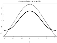
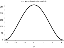
Figure 6.1: Highly conducting case. $k_{1}=1500,k_{2}=1200$, and $\epsilon$ is $0.5,0.01,0.0001$ from left to right. The dashed gray line represents $\partial(u-H)/\partial\nu\bigr{|}^{+}_{\partial B_{1}}$ while the black line does $Q_{\partial B_{1}}$.

Example 2. In this example, we set $\epsilon=0.01$ and $H(\mathbf{x})=x$. The conductivities are $(k_{1},k_{2})=(7,5),(70,50),(7000,5000)$. In Figure 6.2, we plot $\partial(u-H)/\partial\nu\bigr{|}^{+}_{\partial B_{1}}$ and $Q_{\partial B_{1}}$ in gray and black, respectively. The difference between two terms are remained almost unchanged.

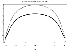
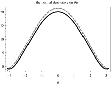
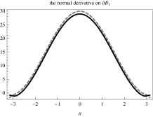
Figure 6.2: The distance $\epsilon$ is fixed to be 0.01, and conductivities are $(k_{1},k_{2})$ is $(7,5),(70,50),(7000,5000)$ from left to right.

Example 3. In this example, we draw the equipotential lines for the singular term in $u$ and $|\nabla u|$ outside inclusions when the circular inclusions are highly conducting or almost insulating. More precisely, we set $(k_{1},k_{2})=(100,200),(0.03,0.02)$ and fix $\epsilon=0.1$. The background potential $H(\mathbf{x})$ is $x$ for highly conducting inclusions and $y$ for almost insulating ones.

In Figure 6.3, we show contour plot of $\Re\{q\}$ and $\bigr{|}\Re\{\nabla q\}\bigr{|}$ which are singular terms of $u$ and $|\nabla u|$, respectively. For both cases, in the narrow region between the inclusions, $|\nabla u|$ changes fast in $y$-direction but slowly in $x$-direction which is in accordance with Proposition 4.2. Away from the touching region, $|\nabla u|$ changes slowly, see Lemma 4.6. The contour of $|\nabla u|$ is continuous across the boundary of inclusions for almost insulating case while it is discontinuous for highly conducting, and $|\nabla u|$ blows-up inside inclusions for almost insulating case while it is bounded for highly conducting case as $\epsilon$ goes to zero.

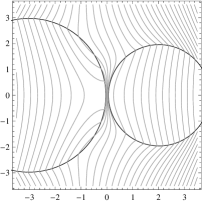
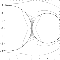
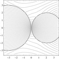
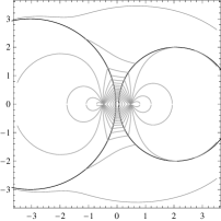
Figure 6.3: Contour plot of the singular term of $u$, the first column, and of $|\nabla u|$, the second column. Inclusions are either highly conducting, the first row, or almost insulating, the second row.

References

- [1] H. Ammari, G. Ciraolo, H. Kang, H. Lee, and K. Yun, Spectral analysis of the Neumann-Poincaré operator and characterization of the stress blow-up in anti-plane elasticity. Archive on Rational Mechanics and Analysis, 208 (2013), 275-304.
- [2] H. Ammari, H. Kang, H. Lee, J. Lee and M. Lim, Optimal bounds on the gradient of solutions to conductivity problems, J. Math. Pures Appl. 88 (2007), 307–324.
- [3] H. Ammari, H. Kang, H. Lee, M. Lim and H. Zribi, Decomposition theorems and fine estimates for electrical fields in the presence of closely located circular inclusions, Jour. Diff. Equa., 247 (2009), 2897-2912.
- [4] H. Ammari, H. Kang and M. Lim, Gradient estimates for solutions to the conductivity problem, Math. Ann. 332(2) (2005), 277-286.
- [5] I. Babus̆ka, B. Andersson, P. Smith and K. Levin, Damage analysis of fiber composites. I. Statistical analysis on fiber scale, Comput. Methods Appl. Mech. Engrg. 172 (1999), 27–77.
- [6] E.S. Bao, Y.Y. Li, B. Yin, Gradient estimates for the perfect conductivity problem, Arch. Ration. Mech. Anal. 193 (2009), 195-226.
- [7] E.S. Bao, Y.Y. Li and B. Yin, Gradient estimates for the perfect and insulated conductivity problems with multiple inclusions, Comm. Part. Diff. Equa. 35 (2010), 1982–2006.
- [8] E. Bonnetier and F. Triki, Pointwise bounds on the gradient and the spectrum of the Neumann-Poincaré operator: The case of 2 discs, Contemporary Mathematics 577 (2012), 81-91.
- [9] E. Bonnetier and M. Vogelius, An elliptic regularity result for a composite medium with “touching” fibers of circular cross-section, SIAM Jour. Math. Anal. 31 No 3 (2000), 651–677.
- [10] B. Budiansky and G. F. Carrier, High shear stresses in stiff fiber composites, Jour. Appl. Mech. 51 (1984), 733-735.
- [11] Chelo Ferreira, José L. López, Asymptotic Expansions of the Hurwitz-Lerch Zeta Function, Jour. Math. Anal. Appl. 298 (2004), 210-224
- [12] H. Kang, M. Lim and K. Yun, Asymptotics and computation of the solution to the conductivity equation in the presence of adjacent inclusions with extreme conductivities, Jour. Math. Pure Appl. 99 (2013) 234-249.
- [13] H. Kang, M. Lim and K. Yun, Characterization of the electric field concentration between two adjacent spherical perfect conductors, arXiv: 1305.0921
- [14] J.B. Keller, Conductivity of a medium containing a dense array of perfectly conducting spheres or cylinders or nonconducting cylinders, J. Appl. Phys., 34:4 (1963), 991–993.
- [15] Y.Y. Li and L. Nirenberg, Estimates for elliptic system from composite material, Comm. Pure Appl. Math., LVI (2003), 892–925.
- [16] Y.Y. Li and M. Vogelius, Gradient estimates for solution to divergence form elliptic equation with discontinuous coefficients, Arch. Rat. Mech. Anal. 153 (2000), 91–151.
- [17] M. Lim and K. Yun, Blow-up of electric fields between closely spaced spherical perfect conductors, Comm. Part. Diff. Equa. 34 (2009), 1287–1315.
- [18] M. Lim and K. Yun, Strong influence of a small fiber on shear stress in fiber-reinforced composites, Jour. Diff. Equa. 250 (2011), 2402–2439.
- [19] P.M. Morse and H. Feshbach, Methods of Theoretical Physics Parts 2, McGraw Hill, 1953.
- [20] K. Yun, Estimates for electric fields blown up between closely adjacent conductors with arbitrary shape, SIAM Jour. Appl. Math. 67 No 3 (2007), 714–730.
- [21] K. Yun, Optimal bound on high stresses occurring between stiff fibers with arbitrary shaped cross sections, Jour. Math. Anal. Appl. 350 (2009), 306-312.