Quantum statistics of light transmitted through an intracavity Rydberg medium

Abstract

We theoretically investigate the quantum statistical properties of light transmitted through an atomic medium with strong optical non-linearity induced by Rydberg-Rydberg van der Waals interactions. In our setup, atoms are located in a cavity and non-resonantly driven on a two-photon transition from their ground state to a Rydberg level via an intermediate state by the combination of the weak signal field and a strong control beam. To characterize the transmitted light we compute the second-order correlation function $g^{\left(2\right)}\left(\tau\right)$. The simulations we obtained on the specific case of rubidium atoms suggest that the bunched or antibunched nature of the outgoing beam can be chosen at will by appropriately tuning the physical parameters.

I Introduction

In an optically non-linear atomic medium, dispersion and absorption of a classical light beam depend on powers of its amplitude B08 . At the quantum level, dispersive optical non-linearities translate into effective interactions between photons. The ability to achieve such strong quantum optical non-linearities is of prominent importance in quantum communication and computation for it would allow to implement photonic conditional two-qubit gates. The standard Kerr dispersive non linearities obtained in non-interacting atomic ensembles, either in off-resonant two-level or resonant three-level configurations involving Electromagnetically Induced Transparency (EIT), are too small to allow for quantum non-linear optical manipulations. To further enhance such non-linearities, EIT protocols were put forward in which the upper level of the ladder is a Rydberg level. In such schemes, the strong van der Waals interactions between Rydberg atoms result in a cooperative Rybderg blockade phenomenon LFC01 ; SWM10 ; CP10 , where each Rydberg atom prevents the excitation of its neighbors inside a "blockade sphere". This Rydberg blockade deeply changes the EIT profile and leads to magnified non-linear susceptibilities PMG10 ; DK12 ; PFL12 ; MSB13 . In particular, giant dispersive non-linear effects were experimentally obtained in an off-resonant Rydberg-EIT scheme using cold rubidium atoms placed in an optical cavity PBS12 ; SPB13 . In this paper, we theoretically investigate the quantum statistical properties of the light generated in the latter protocol. Note that, contrary to other theoretical works, e.g. GOF11 ; GNP13 , here, we are interested in the dispersive regime. Moreover, since we place the atoms in a cavity rather than in free-space, the theoretical framework and calculations we perform also differ from GOF11 ; GNP13 . In particular, a technical benefit of our approach is that we are not restricted to considering only photon pairs but could, in principle, investigate higher-order correlations.

We first write the dynamical equations for the system of interacting three-level atoms coupled to the strong control field and the non-resonant cavity mode, fed by the probe beam. We show that, under some assumptions, the system effectively behaves as a large spin coupled to the cavity mode GBE10 . We then compute the steady-state second-order correlation function to characterize the emission of photons out of the cavity. Our numerical simulations suggest that the bunched or antibunched nature of the outgoing light as well as its coherence time may be controlled through adjusting the detuning between the cavity mode and probe field frequencies.

The paper is structured as follows. In Sec. II, we present our setup and the assumptions we make to compute its dynamics. We also explain the analytical and numerical methods we employ to calculate the second-order $g^{\left(2\right)}$ correlation function of the outgoing light beam. In Sec. III, we present and interpret the results of the simulations we obtained for $g^{\left(2\right)}\left(0\right)$ and $g^{\left(2\right)}\left(\tau>0\right)$ on the specific experimental case considered in PBS12 . Finally, we conclude in Sec. IV by evoking open questions and perspectives of our work. Appendices address supplementary technical details which are omitted in the text for readability.

II Model and methods

The system we consider comprises $N$ atoms which present a three-level ladder structure with a ground $\left|g\right\rangle$, intermediate $\left|e\right\rangle$ and Rydberg states $\left|r\right\rangle$ (see Fig. II.1). The energy of the atomic level $\left|k=g,e,r\right\rangle$ is denoted by $\hbar\omega_{k}$ (by convention $\omega_{g}=0$) and the dipole decay rates from the intermediate and Rydberg states are denoted by $\gamma_{e}$ and $\gamma_{r}$, respectively. The transitions $\left|g\right\rangle\leftrightarrow\left|e\right\rangle$ and $\left|e\right\rangle\leftrightarrow\left|r\right\rangle$ are respectively driven by a weak probe field of frequency $\omega_{p}$ and a strong control field of frequency $\omega_{cf}$. To limit absorption, both fields are off-resonant, the respective detunings are given by $\Delta_{e}\equiv\left(\omega_{p}-\omega_{e}\right)$ and $\Delta_{r}\equiv\left(\omega_{p}+\omega_{cf}-\omega_{r}\right)$. Moreover, to enhance dispersive effects while keeping a high input-output coupling efficiency, the atoms are placed in an optical low-finesse cavity. The transition $\left|g\right\rangle\leftrightarrow\left|e\right\rangle$ is supposed in the neighbourhood of a cavity resonance. The frequency and annihilation operator of the corresponding mode are denoted by $\omega_{c}$ and $a$, respectively ; the detuning of this mode with the probe laser is defined by $\Delta_{c}\equiv\left(\omega_{p}-\omega_{c}\right)$ and $\alpha$ denotes the feeding rate of the cavity mode with the probe field, which is supposed real for simplicity. Finally, we introduce $g$ and $\Omega_{cf}$ which are the single-atom coupling constant of the transition $\left|g\right\rangle\leftrightarrow\left|e\right\rangle$ with the cavity mode and the Rabi frequency of the control field on the transition $\left|e\right\rangle\leftrightarrow\left|r\right\rangle$, respectively. In the following paragraphs, we study the dynamics of the system which, under some assumptions, is equivalent to a damped harmonic oscillator, i.e. the cavity mode, coupled to an assembly of spins $\frac{1}{2}$, i.e. the Rydberg bubbles corresponding to the "super-atoms" delimited by the Rydberg blockade spheres.

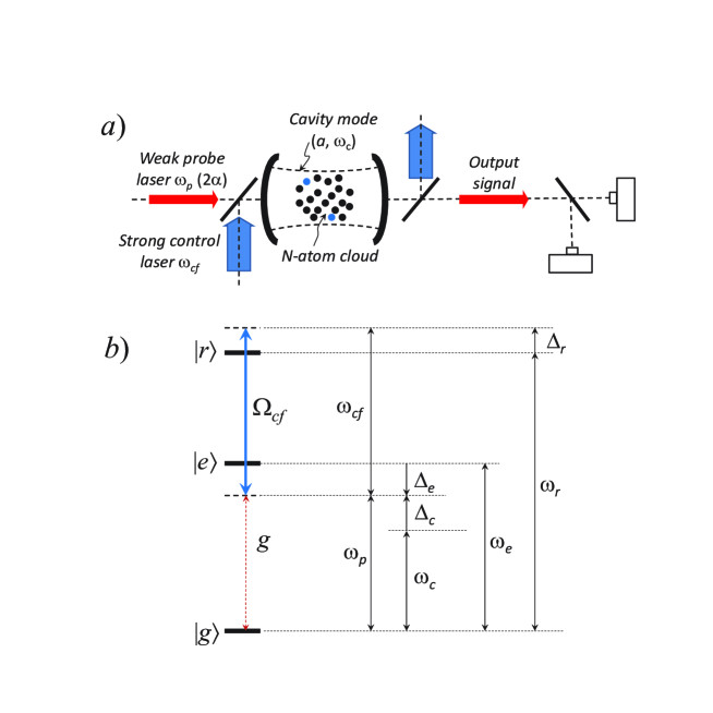
Figure II.1: a) The setup consists of $N$ cold atoms placed in an optical cavity which is fed by a weak (classical) laser beam of frequency $\omega_{p}$ and a strong control laser field of frequency $\omega_{cf}$. b) The atoms present a three-level ladder structure $\left\{\left|g\right\rangle,\left|e\right\rangle,\left|r\right\rangle\right\}$. The transitions $\left|g\right\rangle\leftrightarrow\left|e\right\rangle$ and $\left|e\right\rangle\leftrightarrow\left|r\right\rangle$ are non-resonantly driven by the injected probe and control laser fields, respectively, with the respective coupling strength and Rabi frequency $g$ and $\Omega_{cf}$ (see the text for the definitions of the different detunings represented here).

Starting from the full Hamiltonian, we perform the Rotating Wave Approximation and adiabatically eliminate the intermediate state $\left|e\right\rangle$ as described in Appendix A. Note that the result we obtain coincides with the lowest-order of EIT model – the non-linearity of the three-level atoms is neglected, and the leading non-linear effect comes from the Rydberg-Rydberg collisional effects. The system therefore consists of $N$ effective two-level atoms $\left\{\left|g\right\rangle,\left|r\right\rangle\right\}$, with an effective power-broadened dipole decay rate from the Rydberg level

$$\widetilde{\gamma}_{r}=\left(\gamma_{r}+\frac{\Omega_{cf}^{2}\gamma_{e}}{4\left(\Delta_{e}^{2}+\gamma_{e}^{2}\right)}\right),$$

coupled to the cavity mode of effective decay rate

$$\widetilde{\gamma}_{c}=\left(\gamma_{c}+\frac{g^{2}N\gamma_{e}}{\Delta_{e}^{2}+\gamma_{e}^{2}}\right)$$

increased by the coupling to the atomic ensemble. The Hamiltonian reads

$$\tilde{H} = -\hbar\tilde{\Delta}_{r}\left(\sum_{n=1}^{N}\sigma_{rr}^{\left(n\right)}\right)+\sum_{m<n=1}^{N}\hbar\kappa_{mn}\sigma_{rr}^{\left(m\right)}\sigma_{rr}^{\left(n\right)}$$

$$-\hbar\tilde{\Delta}_{c}a^{\dagger}a+\hbar\alpha\left(a+a^{\dagger}\right)+\hbar g_{\mathrm{eff}}\left\{a\left(\sum_{n=1}^{N}\sigma_{rg}^{\left(n\right)}\right)+h.c.\right\}$$

In this expression, we introduced the atomic operators $\sigma_{kl}^{\left(n\right)}\equiv\mathbb{I}^{\left(1\right)}\otimes\ldots\otimes\mathbb{I}^{\left(n-1\right)}\otimes\left|k\right\rangle\left\langle l\right|\otimes\mathbb{I}^{\left(n+1\right)}\otimes\ldots\otimes\mathbb{I}^{\left(N\right)}$ for $\left(k,l\right)=g,e,r$ as well as the effective detunings

$$\tilde{\Delta}_{r}\equiv\Delta_{r}-\frac{\Omega_{cf}^{2}\Delta_{e}}{4\left(\Delta_{e}^{2}+\gamma_{e}^{2}\right)}$$

and

$$\tilde{\Delta}_{c}\equiv\Delta_{c}-\frac{g^{2}N\Delta_{e}}{\Delta_{e}^{2}+\gamma_{e}^{2}}$$

respectively shifted from $\Delta_{r}$ and $\Delta_{c}$ by the AC Stark shift of the control beam and by the linear atomic susceptibility. The quantity $\kappa_{mn}\equiv C_{6}/\left\|\vec{r}_{m}-\vec{r}_{n}\right\|^{6}$ is the van der Waals interaction between atoms $\left(m,n\right)$ in their Rydberg level – when atoms are in the ground or intermediate states, their interactions are neglected, while

$$g_{\mathrm{eff}}=\frac{g\Omega_{cf}}{2\Delta_{e}}$$

is the effective coupling strength of the two-photon transition $\left|g\right\rangle\rightarrow\left|r\right\rangle$ driven by the cavity mode and the control laser.

At this point, following GBE10 , we introduce the Rydberg bubble approximation. In this approach, the strong Rydberg interactions are assumed to effectively split the sample into ${\cal N}_{b}$ bubbles $\left\{\mathcal{B}_{\alpha=1,\ldots,\mathcal{N}_{b}}\right\}$ each of which contains $n_{b}=\left(\frac{N}{\mathcal{N}_{b}}\right)$ atoms but can only accomodate a single Rydberg excitation, delocalized over the bubble. Note that the number of atoms per bubble $n_{b}$ is approximately given by PBS12

$$n_{b}=\frac{2\pi^{2}\rho_{\mathrm{at}}}{3}\sqrt{\frac{\left|C_{6}\right|}{\Delta_{r}-\Omega_{cf}^{2}/(4\Delta_{e})}}$$

where $\rho_{\mathrm{at}}$ is the atomic density. Each bubble can therefore be viewed as an effective spin $\frac{1}{2}$ whose Hilbert space is spanned by

$$\left|-_{\alpha}\right\rangle=\left|G_{\alpha}\right\rangle \equiv \bigotimes_{i_{\alpha}\in\mathcal{B}_{\alpha}}\left|g_{i_{\alpha}}\right\rangle$$

$$\left|+_{\alpha}\right\rangle=\left|R_{\alpha}\right\rangle \equiv \frac{1}{\sqrt{n_{b}}}\left\{\left|rg\ldots g\right\rangle+\ldots+\left|g\ldots gr\right\rangle\right\}$$

the ground state of the bubble $\mathcal{B}_{\alpha}$ and its symmetric singly Rydberg excited state, respectively. Introducing the bubble spin-$\frac{1}{2}$ operators $\mathrm{s}_{-}^{\left(\alpha\right)}=\hbar\left|-_{\alpha}\right\rangle\left\langle+_{\alpha}\right|$ – the operator $\mathrm{s}_{-}^{\left(\alpha\right)}$ corresponds to the lowering operator of the spin and the annihilation of a Rydberg excitation, one can write the Hamiltonian under the approximate form (see Appendix A)

$$\tilde{H} \approx -\hbar\tilde{\Delta}_{c}a^{\dagger}a+\hbar\alpha\left(a+a^{\dagger}\right)$$

$$-\hbar\tilde{\Delta}_{r}\left(\frac{\mathcal{N}_{b}}{2}+\frac{\mathrm{J}_{z}}{\hbar}\right)$$

$$+g_{\mathrm{eff}}\sqrt{n_{b}}\left(a\mathrm{J}_{+}+a^{\dagger}\mathrm{J}_{-}\right)$$

where we introduced the collective angular momentum $\mathrm{J}_{-}\equiv\sum_{\alpha=1}^{\mathcal{N}_{b}}\mathrm{s}_{-}^{\left(\alpha\right)}$. The system is therefore equivalent to a large spin, i.e. the assembly of spin-$\frac{1}{2}$ Rydberg bubbles, coupled to a harmonic oscillator. Its density matrix satisfies the master equation

$$\partial_{t}\tilde{\rho} = \mathcal{L}\tilde{\rho}$$

$$= \frac{1}{\mathrm{i}\hbar}\left[\tilde{H},\tilde{\rho}\right]+\widetilde{\gamma}_{c}\left\{2a\tilde{\rho}a^{\dagger}-a^{\dagger}a\tilde{\rho}-\tilde{\rho}a^{\dagger}a\right\}$$

$$+\widetilde{\gamma}_{r}\sum_{\alpha=1}^{\mathcal{N}_{b}}\left\{2\mathrm{s}_{-}^{\left(\alpha\right)}\tilde{\rho}\mathrm{s}_{+}^{\left(\alpha\right)}-\mathrm{s}_{+}^{\left(\alpha\right)}\mathrm{s}_{-}^{\left(\alpha\right)}\tilde{\rho}-\tilde{\rho}\mathrm{s}_{+}^{\left(\alpha\right)}\mathrm{s}_{-}^{\left(\alpha\right)}\right\}$$

One can also write the Heisenberg-Langevin equations for the time-dependent operators $a\left(t\right),\mathrm{J}_{-}\left(t\right)$

$$\partial_{t}a = \left(\mathrm{i}\tilde{\Delta}_{c}-\tilde{\gamma}_{c}\right)a-\mathrm{i}\alpha+\mathrm{i}g\mathrm{{}_{eff}}\sqrt{n_{b}}\frac{\mathrm{J}_{-}}{\hbar}+\tilde{a}_{in}$$ (II.2)

$$\partial_{t}\mathrm{J}_{-} = \left(\mathrm{i}\tilde{\Delta}_{r}-\tilde{\gamma}_{r}\right)\mathrm{J}_{-}+\mathrm{i}\hbar g\mathrm{{}_{eff}}\sqrt{N\mathcal{N}_{b}}a+\tilde{\mathrm{J}}_{in}$$ (II.3)

where $\tilde{a}_{in},\tilde{\mathrm{J}}_{in}\equiv\sum_{n=1}^{N}\tilde{F}_{gr}^{\left(n\right)}$ are the Langevin forces associated to $a$ and $\mathrm{J}_{-}$, respectively. Note that we neglected the effect of extra dephasing due to, e.g., collisions or laser fluctuations.

To study the quantum properties of the light transmitted through the cavity, we shall compute the function $g_{\mathrm{out}}^{\left(2\right)}$, which characterizes the two-photon correlations. In the input-output formalism Walls , one shows that this function simply equals the function $g^{\left(2\right)}$ for the intra-cavity field (see Appendix B for details) given by

$$g^{\left(2\right)}\left(\tau\right)=\frac{\mathrm{Tr}\left\{a^{\dagger}ae^{\mathcal{L}\tau}\left[a\rho_{ss}a^{\dagger}\right]\right\}}{\mathrm{Tr}\left[a^{\dagger}a\rho_{ss}\right]^{2}}$$ (II.4)

where $\rho_{ss}$ denotes the steady state of the system defined by $\mathcal{L}\rho_{ss}=0$, see Eq. (II).

In the regime of small feeding parameter $\alpha$, one can compute $\rho_{ss}$ numerically by propagating in time the initial state $\rho_{0}\equiv\left|N_{r}=0\right\rangle\left\langle N_{r}=0\right|\otimes\left|n_{c}=0\right\rangle\left\langle n_{c}=0\right|$ (here $\left|N_{r}=0,1,\ldots,\mathcal{N}_{b}\right\rangle$ represents the symmetric state in which $N_{r}\equiv\left(\frac{\mathcal{N}_{b}}{2}+\frac{\mathrm{J}_{z}}{\hbar}\right)$ bubbles are excited, and $\left|n_{c}=0,1,\ldots\right\rangle$ are the Fock states of the cavity mode). To this end, one applies the Liouvillian evolution operator $e^{\mathcal{L}t}$ in a truncated basis, restricted to states of low numbers of excitations (typically with $n_{c}+N_{r}\leq 6$). The steady state is reached in the limit of large times – ideally when $t\rightarrow\infty$. The denominator of the ratio Eq.(II.4) is directly obtained from $\rho_{ss}$. To compute its numerator, one first propagates in time $a\rho_{ss}a^{\dagger}$ from $t=0$ to $\tau$, using the same procedure as above, then applies the operator $a^{\dagger}a$ and takes the trace.

In the regime of weak feeding, it is also possible to get a perturbative expression for $g^{\left(2\right)}\left(0\right)$ by computing the expansion of $\left\langle a^{\dagger}a^{\dagger}aa\right\rangle_{ss}$ and $\left\langle a^{\dagger}a\right\rangle_{ss}$ in powers of $\alpha$. To this end, one uses the Heisenberg equations of the system Eqs.(II.2,II.3) to derive the hierarchy of equations relating the different mean values and correlations $\left\langle\ldots\right\rangle_{ss}$ up to the fourth order in $\alpha$. After straightforward though lengthy algebra, one gets an expression for $g^{\left(2\right)}\left(0\right)$ which is too cumbersome to be reproduced here but allows for faster calculations than the numerical approach. Such a fully analytical treatment, however, cannot, to our knowledge, be extended to $g^{\left(2\right)}\left(\tau>0\right)$; for $\tau>0$ we therefore entirely rely on numerical simulations.

To conclude this section, we consider the regime of large number of bubbles and low number of excitations, i.e. $\mathcal{N}_{b}\gg 1$ and $\frac{\mathrm{J}_{z}}{\hbar}\ll\mathcal{N}_{b}$. As shown in Appendix A, the operator $b\equiv\frac{J_{-}}{\hbar\sqrt{\mathcal{N}_{b}}}$ is then approximately bosonic, and the term $\left(\frac{\mathcal{N}_{b}}{2}+\frac{\mathrm{J}_{z}}{\hbar}\right)$ can be put under the form

$$\left(\frac{\mathcal{N}_{b}}{2}+\frac{\mathrm{J}_{z}}{\hbar}\right) \approx \frac{\mathrm{J}_{+}\mathrm{J}_{-}}{\hbar^{2}\left(\mathcal{N}_{b}+1\right)}+\frac{\left(\mathrm{J}_{+}\mathrm{J}_{-}\right)^{2}}{\hbar^{4}\left(\mathcal{N}_{b}+1\right)^{3}}$$

$$\approx \frac{\mathcal{N}_{b}}{\left(\mathcal{N}_{b}+1\right)}b^{\dagger}b+\frac{\mathcal{N}_{b}^{2}}{\left(\mathcal{N}_{b}+1\right)^{3}}b^{\dagger}bb^{\dagger}b$$

$$\approx b^{\dagger}b+\frac{1}{\mathcal{N}_{b}}b^{\dagger}b^{\dagger}bb$$

Finally, we get the following approximate expression for the effective Hamiltonian

$$\tilde{H} \approx -\hbar\tilde{\Delta}_{c}a^{\dagger}a+\hbar\alpha\left(a+a^{\dagger}\right)-\hbar\tilde{\Delta}_{r}b^{\dagger}b-\frac{\hbar\bar{\kappa}}{2}b^{\dagger}b^{\dagger}bb+\hbar g_{\mathrm{eff}}\sqrt{N}\left(ab^{\dagger}+a^{\dagger}b\right)$$

where $\bar{\kappa}\equiv 2\tilde{\Delta}_{r}/\mathcal{N}_{b}$. In this regime, the system therefore behaves as two coupled oscillators: one is harmonic, the cavity field, the other is anharmonic, the Rydberg bubble field.

In the following section, we present and discuss the results we obtained with the specific system used in PBS12 . It appears that one can choose the bunched or antibunched behaviour of the light transmitted through the cavity by adjusting the detuning $\Delta_{c}$. We also show that the time behaviour of the function $g^{\left(2\right)}\left(\tau\right)$ depends on the regime considered, and can be roughly understood as resulting from the damped exchange of a single excitation between atoms and field.

III Numerical results and discussion

We consider the physical setup presented in PBS12 , i.e. an ensemble of ⁸⁷Rb atoms, whose state space is restricted to the levels $\left|g\right\rangle=\left|5s_{\frac{1}{2}};F=2\right\rangle$, $\left|e\right\rangle=\left|5p_{\frac{3}{2}};F=3\right\rangle$ and $\left|r\right\rangle=\left|95d_{\frac{5}{2}};F=4\right\rangle$ with the decay rates $\gamma_{e}=2\pi\times 3$ MHz, and $\gamma_{r}=2\pi\times 0.03$ MHz. The other physical parameters must be designed so that strong non-linearities may be observed at the single-photon level. In the specific system considered here, we find this is achieved for a cavity decay rate $\gamma_{c}=2\pi\times 1$ MHz, a volume of the sample $V=40\pi\times 15\times 15\mu$m³, a sample density $n_{at}=0.4\mu$m^-3, a control laser Rabi frequency $\Omega_{cf}=10\gamma_{e}$, a cooperativity $C=1000$, a detuning of the intermediate level $\Delta_{e}=-35\gamma_{e}$, a detuning of the Rydberg level $\Delta_{r}=0.4\gamma_{e}$, a cavity feeding rate $\alpha=0.01\gamma_{e}$. For these parameters, the cavity detuning $\Delta_{c}^{\left(0\right)}=-6.1\gamma_{e}$ corresponds to the maximal average number of photons in the cavity. Note that these physical parameters are experimentally realistic and feasible.

Let us first focus on the second-order correlation function at zero time $g^{\left(2\right)}\left(0\right)$, represented on Fig. III.1 a) as a function of the reduced detuning $\theta\equiv\left(\Delta_{c}-\Delta_{c}^{\left(0\right)}\right)/\gamma_{e}$. The numerical and theoretical curves are in such a good agreement for the regime considered that the corresponding curves cannot be distinguished. One notes a strong bunching peak (B) $\theta_{B}=-4.9$ and a deep antibunching area centered on (A) $\theta_{A}=0$. This suggests that around (A), photons are preferably emitted one by one, while around (B) they are preferably emitted by pairs. Note, however, that, as a ratio, $g^{\left(2\right)}\left(0\right)$ gives only information on the relative importance of pair and single-photon emissions. Its peaks therefore do not correspond to maxima of photon pair emission, but to the best compromises between $\left\langle a^{\dagger}a^{\dagger}aa\right\rangle_{ss}$ and $\left\langle a^{\dagger}a\right\rangle_{ss}^{2}$, as can be checked by comparison of Fig. III.1 a) and b). Hence, pair emission might dominate in a regime where the number of photons coming out from the cavity is actually very small.

Figure III.1: a) Second-order correlation function at zero time $g^{\left(2\right)}\left(0\right)$ (numerical and analytical plots coincide), as a function of the reduced detuning $\theta\equiv\left(\Delta_{c}-\Delta_{c}^{\left(0\right)}\right)/\gamma_{e}$. In the neighbourhood of the minimum (A) $\theta_{A}=0$, a strong antibunching region is observed (see inset); a strong bunching area is obtained around the peak (B) $\theta_{B}=-4.9$. b) Average number of pairs $\left\langle a^{\dagger}a^{\dagger}aa\right\rangle_{ss}=\left\langle n\left(n-1\right)\right\rangle_{ss}$ (thin line) and square of the average number of photons $\left\langle a^{\dagger}a\right\rangle_{ss}^{2}=\left\langle n\right\rangle_{ss}^{2}$ in the steady state (thick line). The position of the peak of the correlation function $g^{\left(2\right)}\left(0\right)$ is signaled by a vertical line.

Figure III.2: Temporal behaviour of $g^{\left(2\right)}\left(\tau\right)$ for a) $\theta_{B}=-4.9$ and b) $\theta_{A}=0$ . Note that we chose a dimensionless “time”-variable $\tau\times\gamma_{e}$ on the $x$-axis.

We now investigate the behaviour of $g^{\left(2\right)}\left(\tau>0\right)$ for two different values of the detuning, i.e. $\theta_{B}=-4.9$ and $\theta_{A}=0$ which respectively correspond to the peak (B) and minimum (A) of $g^{\left(2\right)}\left(0\right)$. The numerical simulations we obtained are given in Fig. III.2. The plot relative to (B) exhibits damped oscillations, alternatively showing a bunched $\left(g^{\left(2\right)}\left(\tau\right)>1\right)$ or antibunched $\left(g^{\left(2\right)}\left(\tau\right)<1\right)$ behaviour. The plot corresponding to (A) always remains on the antibunched side, though asymptotically tending to $1$.

The features observed can be understood and satisfactorily accounted for by a simple three-level model. Indeed, due to the weakness of $\alpha$, the system, in its steady state, is expected to contain at most two excitations (either photonic or atomic). After a photon detection at $t=0$, it contains at most one excitation which can be exchanged between the cavity field and atoms, as it has been known for long BOR95 ; BSM96 . In other words, the operator $a\rho_{ss}a^{\dagger}$ can be expanded in the space restricted to the three states $\left\{\left|00\right\rangle\equiv\left|N_{r}=0,n_{c}=0\right\rangle,\left|01\right\rangle\equiv\left|N_{r}=0,n_{c}=1\right\rangle,\left|10\right\rangle\equiv\left|N_{r}=1,n_{c}=0\right\rangle\right\}$ and the effective non-Hermitian Hamiltonian for the system, in this subspace, takes the following form:

$$\mathrm{H}_{3}=\hbar\left[\begin{array}[]{ccc}0&\alpha&0\\ \alpha&-\tilde{\Delta}_{c}-\mathrm{i}\tilde{\gamma}_{c}&g_{\mathrm{eff}}\sqrt{N}\\ 0&g_{\mathrm{eff}}\sqrt{N}&-\tilde{\Delta}_{r}-\mathrm{i}\tilde{\gamma}_{r}\end{array}\right]$$

The oscillatory dynamical behaviour observed for $g^{\left(2\right)}(t)$ in the specific cases (A,B) is correctly recovered by this Hamiltonian, which validates the schematic model we used and suggests it comprises the main physical processes at work.

To conclude this section, it is worth mentioning that the two-boson approximation, though strictly speaking not applicable here – the parameters considered in this section indeed correspond to a number of bubbles $\mathcal{N}_{b}\simeq 2$, yields, however, the qualitative behaviour for $g^{\left(2\right)}\left(0\right)$. The minimum is correctly located, though slightly higher than in the spin model; the antibunching peak is slightly shifted towards positive detunings and is weaker than in the previous treatment. These discrepancies result from too low a value of the non-linearity parameter $\bar{\kappa}$ ; they can be corrected through replacing $\bar{\kappa}=2\tilde{\Delta}/\mathcal{N}_{b}$ by $\bar{\kappa}^{\prime}=2\tilde{\Delta}/\left(\mathcal{N}_{b}-1\right)$ in the two-boson Hamiltonian. We first note that $\bar{\kappa}$ and $\bar{\kappa}^{\prime}$ coincide in the regime of large number of bubbles. Moreover, $\bar{\kappa}^{\prime}$ makes sense in the regime of low number of bubbles: in particular, when $\mathcal{N}_{b}\rightarrow 1$, i.e. when only one bubble is available, the non-linearity, proportional to $\bar{\kappa}^{\prime}$, diverges accordingly, therefore forbidding the boson field to contain more than one excitation. Finally, let us mention that $\bar{\kappa}^{\prime}$ can also be recovered via a perturbative treatment of the full model which will be presented in a future paper.

IV Conclusion

In this work, we studied how the strong Rydberg-Rydberg van der Waals interactions in an atomic medium may affect the quantum statistical properties of an incoming light beam. In our model, atoms are located in a low finesse cavity and subject to a weak signal beam and a strong control field. These two fields non-resonantly drive the transition from the ground to a Rydberg level. The system was shown to effectively behave as a large spin coupled to a damped harmonic oscillator, i.e. the assembly of Rydberg bubbles and the cavity mode, respectively. The strong anharmonicity of the atomic spin affects the quantum statistics of the outgoing light beam. To demonstrate this effect, we performed analytical and numerical calculations of the second-order correlation function $g^{\left(2\right)}\left(\tau\geq 0\right)$. The results we obtained on a specific physical example with rubidium atoms show indeed that the transmitted light presents either bunched or antibunched characters, depending on the detuning between the cavity mode and the probe field. This suggests that, in such a setup, one could design light of arbitrary quantum statistics through appropriately adjusting the physical parameters.

In this work, we performed the Rydberg bubble approximation, which allowed us to derive a tractable effective Hamiltonian. This scheme is, however, questionable: interactions between bubbles are indeed neglected, and the different spatial arrangements of the bubbles in the sample are not considered. Though challenging, it would be interesting to run full simulations of the system, rejecting those states which are too far off-resonant due to Rydberg-Rydberg interactions. Besides validating the assumption of the present work, this would indeed enable us to consider other regimes, such as, for instance, the case of resonant transition towards the Rydberg level. We also implicitly made the assumption that the cavity mode and control beam were homogeneous. Spatial variations should be included in the model and their potential influence studied in a future work. Finally, due to the very weak probe field regime considered in this paper, we only presented results on the function $g^{\left(2\right)}\left(\tau\right)$: the production of $n=3,4,\ldots$ correlated photons is indeed very unlikely. In principle, we can, however, numerically compute $g^{\left(n\right)}\left(\tau\right)$ for any $n>2$, which might be relevant in a future work, if addressing stronger probe fields.

Appendix A Derivation of the effective Hamiltonian

A.1 Rotating Wave Approximation

The full Hamiltonian of the system can be written under the form

$$H = H_{a}+H_{c}+V_{a-c}$$

$$H_{a} = \hbar\omega_{e}\sum_{n=1}^{N}\sigma_{ee}^{\left(n\right)}+\hbar\omega_{r}\sum_{n=1}^{N}\sigma_{rr}^{\left(n\right)}$$

$$+\hbar\Omega_{cf}\cos\left(\omega_{cf}t\right)\sum_{n=1}^{N}\left(\sigma_{re}^{\left(n\right)}+\sigma_{er}^{\left(n\right)}\right)$$

$$+\sum_{m<n=1}^{N}\hbar\kappa_{mn}\sigma_{rr}^{\left(m\right)}\sigma_{rr}^{\left(n\right)}$$

$$H_{c} = \hbar\left[\omega_{c}a^{\dagger}a+2\alpha\cos\left(\omega_{p}t\right)\left(a+a^{\dagger}\right)\right]$$

$$V_{a-c} = \sum_{n=1}^{N}\hbar g\left(a+a^{\dagger}\right)\left(\sigma_{eg}^{\left(n\right)}+\sigma_{ge}^{\left(n\right)}\right)$$

where $\sigma_{\alpha\beta}^{\left(n\right)}\equiv\mathbb{I}^{\left(1\right)}\otimes\ldots\otimes\mathbb{I}^{\left(n-1\right)}\otimes\left|\alpha\right\rangle\left\langle\beta\right|\otimes\mathbb{I}^{\left(n+1\right)}\otimes\ldots\otimes\mathbb{I}^{\left(N\right)}$, $\hbar\omega_{\alpha}$ is the energy of the atomic level $\left|\alpha\right\rangle$ for $\alpha=e,r$ (with the convention $\omega_{g}=0$), and $\kappa_{mn}\equiv\frac{C_{6}}{\left\|\vec{r}_{m}-\vec{r}_{n}\right\|^{6}}$ denotes the van der Waals interaction between atoms in the Rydberg level – when atoms are in the ground or intermediate states, their interactions are neglected.

We switch to the rotating frame defined by $\left|\psi\right\rangle\rightarrow\left|\tilde{\psi}\right\rangle=\exp\left(-\frac{\mathrm{i}t}{\hbar}H_{0}\right)$ where

$$H_{0}\equiv\hbar\omega_{p}a^{\dagger}a+\hbar\omega_{p}\sum_{n=1}^{N}\sigma_{ee}^{\left(n\right)}+\hbar\left(\omega_{p}+\omega_{cf}\right)\sigma_{rr}^{\left(n\right)}$$

and perform the Rotating Wave Approximation to get the new Hamiltonian $\tilde{H}=\tilde{H}_{a}+\tilde{H}_{c}+\tilde{V}_{a-c}$, where

$$\tilde{H}_{a} = -\hbar\Delta_{e}\sum_{n=1}^{N}\sigma_{ee}^{\left(n\right)}-\hbar\Delta_{r}\sum_{n=1}^{N}\sigma_{rr}^{\left(n\right)}$$

$$+\frac{\hbar\Omega_{cf}}{2}\sum_{n=1}^{N}\left(\sigma_{re}^{\left(n\right)}+\sigma_{er}^{\left(n\right)}\right)+\sum_{m<n=1}^{N}\hbar\kappa_{mn}\sigma_{rr}^{\left(m\right)}\sigma_{rr}^{\left(n\right)}$$

$$\tilde{H}_{c} = -\hbar\Delta_{c}a^{\dagger}a+\hbar\alpha\left(a+a^{\dagger}\right)$$

$$\tilde{V}_{a-c} = \sum_{n=1}^{N}\hbar g\left(a\sigma_{eg}^{\left(n\right)}+a^{\dagger}\sigma_{ge}^{\left(n\right)}\right)$$

with the detunings $\Delta_{c}\equiv\left(\omega_{p}-\omega_{c}\right)$, $\Delta_{e}\equiv\left(\omega_{p}-\omega_{e}\right)$, and $\Delta_{r}\equiv\left(\omega_{p}+\omega_{cf}-\omega_{r}\right)$.

The corresponding Heisenberg-Langevin equations are:

$$\frac{d}{dt}a = \left(\mathrm{i}\Delta_{c}-\gamma_{c}\right)a-\mathrm{i}\alpha-\mathrm{i}g\sum_{i}^{N}\sigma_{ge}^{\left(i\right)}+a_{in}$$ (A.1)

$$\frac{d}{dt}\sigma_{ge}^{\left(i\right)} = \left(\mathrm{i}\Delta_{e}-\gamma_{e}\right)\sigma_{ge}^{\left(i\right)}-\mathrm{i}\frac{\Omega_{cf}}{2}\sigma_{gr}^{\left(i\right)}+\mathrm{i}ga\left(\sigma_{ee}^{\left(i\right)}-\sigma_{gg}^{\left(i\right)}\right)+F_{ge}^{\left(i\right)}$$ (A.2)

$$\frac{d}{dt}\sigma_{gr}^{\left(i\right)} = \left(\mathrm{i}\Delta_{r}-\gamma_{r}\right)\sigma_{gr}^{\left(i\right)}-\mathrm{i}\frac{\Omega_{cf}}{2}\sigma_{ge}^{\left(i\right)}+\mathrm{i}ga\sigma_{er}^{\left(i\right)}$$

$$-\mathrm{i}\sigma_{gr}^{\left(i\right)}\sum_{j\neq i}^{N}\kappa_{ij}\sigma_{rr}^{\left(j\right)}+F_{gr}^{\left(i\right)}$$

$$\frac{d}{dt}\sigma_{er}^{\left(i\right)} = \left\{\mathrm{i}\left(\Delta_{r}-\Delta_{e}\right)-\gamma_{er}\right\}\sigma_{er}^{\left(i\right)}+\mathrm{i}\frac{\Omega_{cf}}{2}\left(\sigma_{rr}^{\left(i\right)}-\sigma_{ee}^{\left(i\right)}\right)$$

$$+\mathrm{i}ga^{\dagger}\sigma_{gr}^{\left(i\right)}-\,\mathrm{i}\sigma_{er}^{\left(i\right)}\sum_{j\neq i}^{N}\kappa_{ij}\sigma_{rr}^{\left(j\right)}+F_{er}^{\left(i\right)}$$

where $a_{in}$ and $F_{\alpha\beta}^{\left(i\right)}$ denote Langevin forces.

A.2 Elimination of the intermediate state

Let us now simplify the system. First, one deduces from Eq.(A.1) that $\sigma_{er}$ is of second order in the small feeding constant $\alpha$. The term $a\sigma_{er}^{\left(i\right)}$ can therefore be neglected in Eq.(A.1). Moreover, since the ground state population remains dominant during the evolution of the system we can write $\sigma_{ee}^{\left(i\right)}-\sigma_{gg}^{\left(i\right)}\simeq-\mathbb{I}$ ; from Eq.(A.2), the steady-state solution for $\sigma_{ge}^{\left(i\right)}$ in the far detuned regime is therefore

$$\sigma_{ge}^{\left(i\right)}\simeq\frac{\Omega_{cf}}{2\left(\Delta_{e}+\mathrm{i}\gamma_{e}\right)}\sigma_{gr}^{\left(i\right)}+\frac{g}{\left(\Delta_{e}+\mathrm{i}\gamma_{e}\right)}a+\frac{\mathrm{i}}{\left(\Delta_{e}+\mathrm{i}\gamma_{e}\right)}F_{ge}^{\left(i\right)}$$

Finally, substituting this relation into Eqs.(A.1,A.1) one gets

$$\frac{d}{dt}a = \left(\mathrm{i}\tilde{\Delta}_{c}-\tilde{\gamma}_{c}\right)a-\mathrm{i}\alpha+\mathrm{i}g\mathrm{{}_{eff}}\left(\sum_{i}\sigma_{gr}^{\left(i\right)}\right)+\tilde{a}_{in}$$ (A.5)

$$\frac{d}{dt}\sigma_{gr}^{\left(i\right)} = \left(\mathrm{i}\tilde{\Delta}_{r}-\tilde{\gamma}_{r}\right)\sigma_{gr}^{\left(i\right)}+\mathrm{i}g\mathrm{{}_{eff}}a-\mathrm{i}\sigma_{gr}^{\left(i\right)}\left(\sum_{j\neq i}^{N}\kappa_{ij}\sigma_{rr}^{\left(j\right)}\right)+\tilde{F}_{gr}^{\left(i\right)}$$ (A.6)

where

$$\tilde{\Delta}_{c} = \Delta_{c}-\Delta_{e}\frac{g^{2}N}{\left(\Delta_{e}^{2}+\gamma_{e}^{2}\right)}$$

$$\tilde{\gamma}_{c} = \gamma_{c}+\gamma_{e}\frac{g^{2}N}{\left(\Delta_{e}^{2}+\gamma_{e}^{2}\right)}$$

$$\tilde{\Delta}_{r} = \Delta_{r}-\Delta_{e}\frac{\Omega_{cf}^{2}}{4\left(\Delta_{e}^{2}+\gamma_{e}^{2}\right)}$$

$$\tilde{\gamma}_{r} = \gamma_{r}+\gamma_{e}\frac{\Omega_{cf}^{2}}{4\left(\Delta_{e}^{2}+\gamma_{e}^{2}\right)}$$

$$g\mathrm{{}_{eff}} = \frac{g\Omega_{cf}}{2\left(\Delta_{e}+\mathrm{i}\gamma_{e}\right)}\approx\frac{g\Omega_{cf}}{2\Delta_{e}}$$

are the parameters for the effective two-level model and $\tilde{a}_{in},\tilde{F}_{gr}^{\left(i\right)}$ are the modified Langevin noise operators

$$\tilde{a}_{in} = a_{in}+\frac{g}{\left(\Delta_{e}+\mathrm{i}\gamma_{e}\right)}\sum_{i}F_{ge}^{\left(i\right)}\approx a_{in}+\frac{g}{\Delta_{e}}\sum_{i}F_{ge}^{\left(i\right)}$$

$$\tilde{F}_{gr}^{\left(i\right)} = F_{gr}^{\left(i\right)}+\frac{\Omega_{cf}}{2\left(\Delta_{e}+\mathrm{i}\gamma_{e}\right)}F_{ge}^{\left(i\right)}\approx F_{gr}^{\left(i\right)}+\frac{\Omega_{cf}}{2\Delta_{e}}F_{ge}^{\left(i\right)}$$

Note that, in the absence of collisional terms, one simply recovers the standard three-level EIT susceptibility in the far-detuned regime

$$\frac{da}{dt}=\left(\mathrm{i}\Delta_{c}-\gamma_{c}-\frac{g^{2}N}{\frac{\Omega_{cf}^{2}}{4(\gamma_{r}-\mathrm{i}\Delta_{r})}-\mathrm{i}\Delta_{e}}\right)a-\mathrm{i}\alpha+\tilde{a}_{in}$$

Finally, we get the effective Hamiltonian

$$\tilde{H} = -\hbar\tilde{\Delta}_{r}\left(\sum_{n=1}^{N}\sigma_{rr}^{\left(n\right)}\right)+\sum_{m<n=1}^{N}\hbar\kappa_{mn}\sigma_{rr}^{\left(m\right)}\sigma_{rr}^{\left(n\right)}$$

$$-\hbar\tilde{\Delta}_{c}a^{\dagger}a+\hbar\alpha\left(a+a^{\dagger}\right)+\hbar g_{\mathrm{eff}}\left\{a\left(\sum_{n=1}^{N}\sigma_{rg}^{\left(n\right)}\right)+h.c.\right\}$$

A.3 Rybderg bubble approximation

As described in the main text, we introduce the Rydberg bubble approximation. In this approach, the strong Rydberg interactions are assumed to effectively split the sample into ${\cal N}_{b}$ bubbles $\left\{\mathcal{B}_{\alpha=1,\ldots,\mathcal{N}_{b}}\right\}$ each of which contains $n_{b}=\left(\frac{N}{\mathcal{N}_{b}}\right)$ atoms but can only accomodate a single Rydberg excitation, delocalized over the bubble. Note that the number of atoms per bubble $n_{b}$ is approximately given by PBS12

$$n_{b}=\frac{2\pi^{2}\rho_{\mathrm{at}}}{3}\sqrt{\frac{\left|C_{6}\right|}{\Delta_{r}-\Omega_{cf}^{2}/(4\Delta_{e})}}$$

where $\rho_{\mathrm{at}}$ is the atomic density. Each bubble can therefore be viewed as an effective spin $\frac{1}{2}$ whose Hilbert space is spanned by

$$\left|-_{\alpha}\right\rangle=\left|G_{\alpha}\right\rangle \equiv \bigotimes_{i_{\alpha}\in\mathcal{B}_{\alpha}}\left|g_{i_{\alpha}}\right\rangle$$

$$\left|+_{\alpha}\right\rangle=\left|R_{\alpha}\right\rangle \equiv \frac{1}{\sqrt{n_{b}}}\left\{\left|rg\ldots g\right\rangle+\ldots+\left|g\ldots gr\right\rangle\right\}$$

the ground state of the bubble $\mathcal{B}_{\alpha}$ and its symmetric singly Rydberg excited state, respectively. Introducing the bubble Pauli operators $\mathrm{s}_{-}^{\left(\alpha\right)}=\hbar\left|-_{\alpha}\right\rangle\left\langle+_{\alpha}\right|$ – the operator $\mathrm{s}_{-}^{\left(\alpha\right)}$ corresponds to the lowering operator of the spin and the annihilation of a Rydberg excitation, one can write

$$\sum_{n=1}^{N}\sigma_{gr}^{\left(n\right)} = \sum_{\alpha=1}^{\mathcal{N}_{b}}\sum_{i_{\alpha}\in\mathcal{B}_{\alpha}}\sigma_{gr}^{\left(i_{\alpha}\right)}$$

$$\approx \sum_{\alpha=1}^{\mathcal{N}_{b}}\frac{\mathrm{s}_{-}^{\left(\alpha\right)}}{\hbar}\left\langle-_{\alpha}\left|\sum_{i_{\alpha}\in\mathcal{B}_{\alpha}}\sigma_{gr}^{\left(i_{\alpha}\right)}\right|+_{\alpha}\right\rangle$$

$$\approx \sqrt{n_{b}}\sum_{\alpha=1}^{\mathcal{N}_{b}}\frac{\mathrm{s}_{-}^{\left(\alpha\right)}}{\hbar}$$

$$= \sqrt{n_{b}}\frac{\mathrm{J}_{-}}{\hbar}$$

where we introduced the collective angular momentum $\mathrm{J}_{-}\equiv\sum_{\alpha=1}^{\mathcal{N}_{b}}\mathrm{s}_{-}^{\left(\alpha\right)}$. In the same way,

$$\sum_{n=1}^{N}\sigma_{rr}^{\left(n\right)} = \sum_{\alpha=1}^{\mathcal{N}_{b}}\sum_{i_{\alpha}\in\mathcal{B}_{\alpha}}\sigma_{rr}^{\left(i_{\alpha}\right)}$$

$$\approx \sum_{\alpha=1}^{\mathcal{N}_{b}}\left|+_{\alpha}\right\rangle\left\langle+_{\alpha}\right|\left\langle+_{\alpha}\left|\sum_{i_{\alpha}\in\mathcal{B}_{\alpha}}\sigma_{rr}^{\left(i_{\alpha}\right)}\right|+_{\alpha}\right\rangle$$

$$\approx \sum_{\alpha=1}^{\mathcal{N}_{b}}\left(\frac{1}{2}+\frac{\mathrm{s}_{z}^{\left(\alpha\right)}}{\hbar}\right)$$

$$\approx \left(\frac{\mathcal{N}_{b}}{2}+\frac{\mathrm{J}_{z}}{\hbar}\right)$$

where we used $\left|+_{\alpha}\right\rangle\left\langle+_{\alpha}\right|\equiv\left(\frac{1}{2}+\frac{\mathrm{s}_{z}^{\left(\alpha\right)}}{\hbar}\right)$. Finally, the Hamiltonian of the system takes the approximate form

$$\tilde{H} \approx -\hbar\tilde{\Delta}_{c}a^{\dagger}a+\hbar\alpha\left(a+a^{\dagger}\right)$$

$$-\hbar\tilde{\Delta}_{r}\left(\frac{\mathcal{N}_{b}}{2}+\frac{\mathrm{J}_{z}}{\hbar}\right)$$

$$+g_{\mathrm{eff}}\sqrt{\mathcal{N}_{b}}\left(a\mathrm{J}_{+}+a^{\dagger}\mathrm{J}_{-}\right)$$

which represents the interaction of the large spin $\mathrm{J}_{-}$ with the cavity mode $a$.

A.4 Regime of large number of bubbles and low number of excitations

From the well-known relation $\mathrm{J}_{+}\mathrm{J}_{-}=\vec{\mathrm{J}}^{2}-\mathrm{J}_{z}^{2}+\hbar\mathrm{J}_{z}$ we deduce the second-order operator equation

$$\mathrm{J}_{z}^{2}-\hbar\mathrm{J}_{z}-\hbar^{2}\frac{\mathcal{N}_{b}}{2}\left(\frac{\mathcal{N}_{b}+2}{2}\right)+\mathrm{J}_{+}\mathrm{J}_{-}=0$$

In the regime of large number of bubbles $\mathcal{N}_{b}\gg 1$ and for low excitation numbers, i.e. eigenstates of the total angular momentum $\left|j=\frac{\mathcal{N}_{b}}{2};m=-\frac{\mathcal{N}_{b}}{2}+k\right\rangle$ with $k\ll\mathcal{N}_{b}$, the solution of this equation is approximately given by

$$\mathrm{J}_{z}\approx\hbar\left\{-\frac{\mathcal{N}_{b}}{2}+\frac{\mathrm{J}_{+}\mathrm{J}_{-}}{\hbar^{2}\left(\mathcal{N}_{b}+1\right)}+\frac{\left(\mathrm{J}_{+}\mathrm{J}_{-}\right)^{2}}{\hbar^{4}\left(\mathcal{N}_{b}+1\right)^{3}}\right\}$$

whence, at the lowest order in the excitation number,

$$\left(\frac{\mathcal{N}_{b}}{2}+\frac{\mathrm{J}_{z}}{\hbar}\right) \approx \frac{\mathrm{J}_{+}\mathrm{J}_{-}}{\hbar^{2}\left(\mathcal{N}_{b}+1\right)}+\frac{\left(\mathrm{J}_{+}\mathrm{J}_{-}\right)^{2}}{\hbar^{4}\left(\mathcal{N}_{b}+1\right)^{3}}$$ (A.7)

$$\left[\mathrm{J}_{+},\mathrm{J}_{-}\right] \approx -\hbar^{2}\mathcal{N}_{b}$$ (A.8)

Injecting Eq.(A.7) into the previous form of the Hamiltonian we get

$$\tilde{H} \approx -\hbar\tilde{\Delta}_{c}a^{\dagger}a+\hbar\alpha\left(a+a^{\dagger}\right)$$

$$-\hbar\tilde{\Delta}_{r}\left(\frac{\mathrm{J}_{+}\mathrm{J}_{-}}{\hbar^{2}\left(\mathcal{N}_{b}+1\right)}+\frac{\left(\mathrm{J}_{+}\mathrm{J}_{-}\right)^{2}}{\hbar^{4}\left(\mathcal{N}_{b}+1\right)^{3}}\right)$$

$$+\hbar g_{\mathrm{eff}}\sqrt{N}\left(a\frac{\mathrm{J}_{+}}{\hbar\sqrt{\mathcal{N}_{b}}}+a^{\dagger}\frac{\mathrm{J}_{-}}{\hbar\sqrt{\mathcal{N}_{b}}}\right)$$

Moreover, from Eq.(A.8) we deduce that the operator $b\equiv\frac{J_{-}}{\hbar\sqrt{\mathcal{N}_{b}}}$ is approximately bosonic and therefore, the Hamiltonian can finally be put under the form

$$\tilde{H} \approx -\hbar\tilde{\Delta}_{c}a^{\dagger}a+\hbar\alpha\left(a+a^{\dagger}\right)-\hbar\tilde{\Delta}_{r}b^{\dagger}b-\frac{\hbar\bar{\kappa}}{2}b^{\dagger}b^{\dagger}bb+\hbar g_{\mathrm{eff}}\sqrt{N}\left(ab^{\dagger}+a^{\dagger}b\right)$$

where $\bar{\kappa}\equiv 2\tilde{\Delta}_{r}/\mathcal{N}_{b}$.

Appendix B Calculation of $g_{\mathrm{out}}^{\left(2\right)}$

By definition, the second-order correlation function for the outgoing field is

$$g_{out}^{\left(2\right)}(t_{1},t_{2})=\frac{\left\langle a_{out}^{\dagger}\left(t_{1}\right)a_{out}^{\dagger}\left(t_{2}\right)a_{out}\left(t_{2}\right)a_{out}\left(t_{1}\right)\right\rangle}{\left\langle a_{out}^{\dagger}\left(t_{2}\right)a_{out}\left(t_{2}\right)\right\rangle\left\langle a_{out}^{\dagger}\left(t_{1}\right)a_{out}\left(t_{1}\right)\right\rangle}$$

Using the relations Walls

$$\left\langle a_{out}^{\dagger}\left(t\right)a_{out}\left(t\right)\right\rangle = 2\gamma_{c}\left\langle a^{\dagger}\left(t\right)a\left(t\right)\right\rangle$$

$$a_{out}\left(t\right) = \sqrt{2\gamma_{c}}a\left(t\right)-a_{in}\left(t\right)$$

and keeping only non-zero terms (all terms like $\left\langle a_{in}^{\dagger}....\right\rangle$ and $\left\langle....a_{in}\right\rangle$ equal zero), one obtains in the numerator four non-zero terms

$$\left\langle a^{\dagger}(t_{1})a^{\dagger}(t_{2})a_{in}(t_{2})a(t_{1})\right\rangle$$

$$\left\langle a^{\dagger}(t_{1})a^{\dagger}(t_{2})a(t_{2})a(t_{1})\right\rangle$$

$$\left\langle a^{\dagger}(t_{1})a_{in}^{\dagger}(t_{2})a(t_{2})a(t_{1})\right\rangle$$

$$\left\langle a^{\dagger}(t_{1})a_{in}^{\dagger}(t_{2})a_{in}(t_{2})a(t_{1})\right\rangle$$

Let us consider the first term. Using the standard commutation relations between $a$ and $a_{in}$ operators we have:

$$\left\langle a^{\dagger}(t_{1})a^{\dagger}(t_{2})a_{in}(t_{2})a(t_{1})\right\rangle = \left\langle a^{\dagger}(t_{1})a^{\dagger}(t_{2})a(t_{1})a_{in}(t_{2})\right\rangle$$

$$+\left\langle a^{\dagger}(t_{1})a^{\dagger}(t_{2})\left[a_{in}(t_{2}),a(t_{1})\right]\right\rangle$$

$$= \sqrt{2\gamma_{c}}\theta(t_{1}-t_{2})\left\langle a^{\dagger}(t_{1})a^{\dagger}(t_{2})\left[a(t_{2}),a(t_{1})\right]\right\rangle$$

Here we used the relation

$$\left[X\left(t_{1}\right),a_{in}\left(t_{2}\right)\right]=\sqrt{2\gamma_{c}}\theta\left(t_{1}-t_{2}\right)\left[X,a\right]$$

where $X$ is any system operator Walls and where $\theta\left(\tau\right)$ is the Heaviside step-function (with $\theta\left(0\right)=\frac{1}{2}$).

Evaluating the other terms in the same way one finally obtains

$$g_{out}^{(2)}\left(t_{1},t_{2}\right)=\frac{\left\langle a^{\dagger}\left(t_{m}\right)a^{\dagger}\left(t_{M}\right)a\left(t_{M}\right)a\left(t_{m}\right)\right\rangle}{\left\langle a^{\dagger}\left(t_{1}\right)a\left(t_{1}\right)\right\rangle\left\langle a^{\dagger}\left(t_{2}\right)a\left(t_{2}\right)\right\rangle}$$

where $t_{m}\equiv\mathrm{min}\left(t_{1},t_{2}\right)$ and $t_{M}\equiv\mathrm{max}\left(t_{1},t_{2}\right)$.

References

• (1) Boyd R W 2008 Nonlinear Optics 3rd ed. (Academic Press, USA).
• (2) Lukin M D, Fleischhauer M, Cᅵtᅵ R, Duan L M, Jaksch D, Cirac J I, and Zoller P 2001 Dipole Blockade and Quantum Information Processing in Mesoscopic Atomic Ensembles Phys. Rev. Lett. 87, 037901.
• (3) Saffman M, Walker T G, and Moelmer K 2010 Quantum information with Rydberg atoms Rev. Mod. Phys. 82, 2313.
• (4) Comparat D and Pillet P 2010 Dipole blockade in a cold Rydberg atomic sample J. Opt. Soc. Am. B 27, A208.
• (5) Pritchard J D, Maxwell D, Gauguet A, Weatherill K J, Jones M P A, and Adams C S 2010 Cooperative Atom-Light Interaction in a Blockaded Rydberg Ensemble Phys. Rev. Lett. 105, 193603
• (6) Dudin Y O and Kuzmich A 2012 Strongly Interacting Rydberg Excitations of a Cold Atomic Gas Science 336, 887
• (7) Peyronel T, Firstenberg O, Liang Q Y, Hofferberth S, Gorshkov A V, Pohl T, Lukin M D and Vuletic V 2012 Quantum nonlinear optics with single photons enabled by strongly interacting atoms Nature 488, 57
• (8) Maxwell D, Szwer D J, Barato D P, Busche H, Pritchard J D, Gauguet A, Weatherill K J, Jones M P A, and Adams C S 2013 Storage and Control of Optical Photons Using Rydberg Polaritons Phys. Rev. Lett. 110, 103001
• (9) Parigi V, Bimbard E, Stanojevic J, Hilliard A J, Nogrette F, Tualle-Brouri R, Ourjoumtsev A, and Grangier P 2012 Observation and Measurement of Interaction-Induced Dispersive Optical Nonlinearities in an Ensemble of Cold Rydberg Atoms Phys. Rev. Lett. 109, 233602
• (10) Stanojevic J, Parigi V, Bimbard E, Ourjoumtsev A, and Grangier P 2013 Dispersive optical nonlinearities in an EIT-Rydberg medium Preprint arXiv:1303.4927
• (11) Gorshkov A V, Otterbach J, Fleischhauer M, Pohl T, and Lukin M D 2011 Photon-Photon Interactions via Rydberg Blockade Phys. Rev. Lett. 107, 133602
• (12) Gorshkov A V, Nath R, and Pohl T 2013 Dissipative Many-Body Quantum Optics in Rydberg Media Phys. Rev. Lett. 110, 153601
• (13) Guerlin C, Brion E, Esslinger T, and Moelmer K 2010 Cavity quantum electrodynamics with a Rydberg-blocked atomic ensemble Phys. Rev. A 82, 053832
• (14) Walls D F and Milburn G J 2008 Quantum Optics 2nd ed. (Springer-Verlag Berlin Heidelberg)
• (15) Brecha R J, Orozco L A, Raizen M G, Xiao M, and Kimble H J 1995 Observation of oscillatory energy exchange in a coupled atom cavity system J. Opt. Soc. Am. B 12, 2329
• (16) Brune M, Schmidt-Kaler F, Maali A, Dreyer J, Hagley E, Raimond J M, and Haroche S 1996 Quantum Rabi Oscillation: A Direct Test of Field Quantization in a Cavity Phys. Rev. Lett. 76, 1800