The GPDs of the photon

Abstract:

We report on a recent calculation of the generalized parton distributions (GPDs) of the photon when the momentum transfer in the transverse direction is non-zero. We use an overlap representation of the photon GPDs in terms of the photon light-front wave functions. We calculate the GPDs at leading order in electromagnetic coupling $\alpha$ and zeroth order in strong coupling $\alpha_{s}$. We consider also the case when the helicity of the photon is flipped. Fourier transform of the GPDs with respect to the transverse momentum transfer gives the parton distributions of the photon in impact parameter space.

1 Introduction

The partonic substructure of the photon play an important role in high energy scattering experiments where the virtuality of the photon involved is very large. The pointlike component of the photon structure function, which is relevant in processes like $e^{+}e^{-}$ annihilation and photoproduction, can be calculated perturbatively. A striking feature of the photon parton distribution is that they have logarithmic scale dependence already at zeroth order of the strong coupling constant unlike the parton distributions of the nucleon. The photon structure functions are now well known both theoretically and experimentally. In [1] the authors have considered deeply virtual Compton scattering on a photon target $\gamma^{*}\gamma\to\gamma\gamma$ in the kinematical region of large center-of-mass energy, large virtuality $(Q^{2})$ but small squared momentum transfer $(-t)$ from the initial to final photon. They interpreted the results in terms of the generalized parton distributions (GPDs) of the photon at leading logarithmic order, in analogy with the GPDs of the proton. At leading order in $\alpha$ and zeroth order in $\alpha_{s}$ the GPDs of the photon depend on the scale logarithmically. These can be calculated perturbatively, unlike the proton GPDs, and they can act as theoretical laboratories to understand the basic properties of GPDs like polynomiality and positivity. In [2] the GPDs of the photon have been used to investigate the analyticity properties of DVCS amplitudes and related sum rules of the GPDs. Recently we have investigated the GPDs of the photon using overlaps of light-front wave functions (LFWFs) of the photon. We extended the study in [1] to a more general kinematics when the momentum transfer between the initial and the final photon also has a transverse component. We have shown that in this kinematics Fourier transform of the photon GPDs give impact parameter dependent parton distribution of the photon in transverse position space. As is known in the DVCS process involving a proton, the helicity of the proton may or may not flip. When the helicity of the proton is flipped, the DVCS amplitude is given in terms of the GPD $E$. The flip needs non-zero orbital angular momentum (OAM) of the overlapping LFWFs of the proton, and is not possible unless there is non-zero momentum transfer in the transverse direction. When the nucleon is transversely polarized, this results in a distortion in the parton distributions in the impact parameter space. We have shown that the photon GPDs where the helicity of the photon is flipped are related to a similar distortion of the parton distributions of the photon in the transverse impact parameter space which is due to the non-vanishing OAM of the partonic constituents of the photon.

2 GPDs of the photon without helicity flip

The GPDs for the photon can be written as the following off-forward matrix elements [1]:

$$F^{q}=\int{dy^{-}\over 8\pi}e^{-iP^{+}y^{-}\over 2}\langle\gamma(P^{\prime},\lambda^{\prime})\mid{\bar{\psi}}(0)\gamma^{+}\psi(y^{-})\mid\gamma(P,\lambda)\rangle;$$

$$\tilde{F}^{q}=\int{dy^{-}\over 8\pi}e^{-iP^{+}y^{-}\over 2}\langle\gamma(P^{\prime},\lambda^{\prime})\mid{\bar{\psi}}(0)\gamma^{+}\gamma^{5}\psi(y^{-})\mid\gamma(P,\lambda)\rangle.$$ (1)

$F^{q}$ contributes when the photon is unpolarized and $\tilde{F}^{q}$ is the contribution from the polarized photon. We have chosen the light-front gauge $A^{+}=0$ and used light-front coordinates. In this section, we take $\lambda^{\prime}=\lambda$ so that there is no helicity flip of the photon. We use the Fock space expansion of a real photon of momentum $P$ and helicity $\lambda$, which can be written as,

$$\mid\gamma(P,\lambda)\rangle = \Big{[}a^{\dagger}(P,\lambda)\mid 0\rangle+\sum_{\sigma_{1},\sigma_{2}}\int\{dk_{1}\}\int\{dk_{2}\}\sqrt{2{(2\pi)}^{3}P^{+}}\delta^{3}(P-k_{1}-k_{2})$$ (2)

$$~{}~{}~{}~{}\phi_{2}(k_{1},k_{2},\sigma_{1},\sigma_{2})b^{\dagger}(k_{1},\sigma_{1})d^{\dagger}(k_{2},\sigma_{2})\mid 0\rangle\Big{]}$$

$\{dk\}=\int{dk^{+}d^{2}k^{\perp}\over\sqrt{2{(2\Pi)}^{3}k^{+}}}$, $\phi_{2}$ is the two-particle ($q\bar{q}$) light-front wave function (LFWF) and $\sigma_{1}$ and $\sigma_{2}$ are the helicities of the quark and antiquark. The wave function can be expressed in terms of Jacobi momenta $x_{i}={k_{i}^{+}\over P^{+}}$ and $q_{i}^{\perp}=k_{i}^{\perp}-x_{i}P^{\perp}$. These obey the relations $\sum_{i}x_{i}=1,\sum_{i}q_{i}^{\perp}=0$. The boost invariant photon LFWFs are given by ${\psi_{2}(x_{i},q_{i}^{\perp})=\phi_{2}\sqrt{P^{+}}}$. $\psi_{2}(x_{i},q_{i}^{\perp})$ can be calculated order by order in perturbation theory [3]. The above off-forward matrix elements can be calculated analytically using these LFWFs [4] and can be written as:

$$F^{q} = \sum_{q}{\alpha e_{q}^{2}\over 4{\pi}^{2}}\Big{[}((1-x)^{2}+x^{2})(I_{1}+I_{2}+LI_{3})+2m^{2}I_{3}\big{]}\theta(x)\theta(1-x)$$ (3)

$$~{}~{}-\sum_{q}{\alpha e_{q}^{2}\over 4{\pi}^{2}}\Big{[}((1+x)^{2}+x^{2})(I^{\prime}_{1}+I^{\prime}_{2}+L^{\prime}I^{\prime}_{3})+2m^{2}I^{\prime}_{3}\Big{]}\theta(-x)\theta(1+x)$$

Here the sum indicates sum over different quark flavors; $L=-2m^{2}+2m^{2}x(1-x)-{(\Delta^{\perp})}^{2}(1-x)^{2}$, $L^{\prime}=-2m^{2}-2m^{2}x(1+x)-{(\Delta^{\perp})}^{2}(1+x)^{2}$; the integrals can be written as,

$$I_{1}=\int{d^{2}q^{\perp}\over D}=\pi Log\Big{[}{\Lambda^{2}\over\mu^{2}-m^{2}x(1-x)+m^{2}}\Big{]}=I_{2}$$

$$I_{3}=\int{d^{2}q^{\perp}\over DD^{\prime}}=\int_{0}^{1}d\alpha{\pi\over P(x,\alpha,{(\Delta^{\perp})}^{2})}$$ (4)

where $D={(q^{\perp})}^{2}-m^{2}x(1-x)+m^{2}$ and $D^{\prime}={(q^{\perp})}^{2}+{(\Delta^{\perp})}^{2}(1-x)^{2}-2q^{\perp}\cdot\Delta^{\perp}(1-x)-m^{2}x(1-x)+m^{2}$, and $P(x,\alpha,{(\Delta^{\perp})}^{2})=-m^{2}x(1-x)+m^{2}+\alpha(1-\alpha)(1-x)^{2}{(\Delta^{\perp})}^{2}$. At zeroth order in $\alpha_{s}$ the results depend on the scale logarithmically. $\mu$ is a lower cutoff on the transverse momentum, which can be taken to zero as long as the quark mass is nonzero.

For the antiquark contributions we have similar integrals

$$I^{\prime}_{1}=\int{d^{2}q^{\perp}\over H}=\pi Log\Big{[}{\Lambda^{2}\over\mu^{2}+m^{2}x(1+x)+m^{2}}\Big{]}=I^{\prime}_{2}$$

$$I^{\prime}_{3}=\int{d^{2}q^{\perp}\over HH^{\prime}}=\int_{0}^{1}d\alpha{\pi\over Q(x,\alpha,{(\Delta^{\perp})}^{2})}$$ (5)

where $H={(q^{\perp})}^{2}+m^{2}x(1+x)+m^{2}$ and $H^{\prime}={(q^{\perp})}^{2}+{(\Delta^{\perp})}^{2}(1+x)^{2}+2q^{\perp}\cdot\Delta^{\perp}(1+x)+m^{2}x(1+x)+m^{2}$, and $Q(x,\alpha,{(\Delta^{\perp})}^{2})=m^{2}x(1+x)+m^{2}+\alpha(1-\alpha)(1+x)^{2}{(\Delta^{\perp})}^{2}$.

For polarized photon the GPD $\tilde{F}^{q}$ can be calculated from the terms of the form $\epsilon^{2}_{\lambda}\epsilon^{1*}_{\lambda}-\epsilon^{1}_{\lambda}\epsilon^{2*}_{\lambda}$ [1]. We consider the terms where the photon helicity is not flipped. This can be written as,

$$\tilde{F}^{q} = \sum_{q}{\alpha e_{q}^{2}\over 4{\pi}^{2}}\Big{[}(x^{2}-(1-x)^{2})(I_{1}+I_{2}+LI_{3})+2m^{2}I_{3}\big{]}\theta(x)\theta(1-x)$$ (6)

$$+\sum_{q}{\alpha e_{q}^{2}\over 4{\pi}^{2}}\Big{[}(x^{2}-(1+x)^{2})(I^{\prime}_{1}+I^{\prime}_{2}+L^{\prime}I^{\prime}_{3})+2m^{2}I^{\prime}_{3}\Big{]}\theta(-x)\theta(1+x)$$

In analogy with the impact parameter dependent parton distribution of the proton [5], we introduce the same for the photon. By taking a Fourier transform with respect to the transverse momentum transfer $\Delta^{\perp}$ we get the GPDs in the transverse impact parameter space.

$$q(x,b^{\perp}) = {1\over(2\pi)^{2}}\int d^{2}\Delta^{\perp}e^{-i\Delta^{\perp}\cdot b^{\perp}}F^{q}$$ (7)

$$= {1\over 2\pi}\int\Delta d\Delta J_{0}(\Delta b)F^{q};$$

$$\tilde{q}(x,b^{\perp}) = {1\over(2\pi)^{2}}\int d^{2}\Delta^{\perp}e^{-i\Delta^{\perp}\cdot b^{\perp}}\tilde{F}^{q}$$ (8)

$$= {1\over 2\pi}\int\Delta d\Delta J_{0}(\Delta b)\tilde{F}^{q};$$

where $J_{0}(z)$ is the Bessel function; $\Delta=|\Delta^{\perp}|$ and $b=|b^{\perp}|$. In the numerical calculation, we have introduced a maximum limit $\Delta_{max}$ of the $\Delta$ integration which we restrict to satisfy the kinematics $-t<<Q^{2}$ [6, 7, 8, 9]. $q(x,b^{\perp})$ gives the distribution of partons in this case inside the photon in the transverse plane. Like the proton, this interpretation holds in the infinite momentum frame and there is no relativistic correction to this identification because in light-front formalism, as well as in the infinite momentum frame, the transverse boosts act like non-relativistic Galilean boosts. $q(x,b^{\perp})$ gives simultaneous information about the longitudinal momentum fraction $x$ and the transverse distance $b$ of the parton from the center of the photon and thus gives a new insight to the internal structure of the photon. The impact parameter distribution for a polarized photon is given by $\tilde{q}(x,b^{\perp})$.

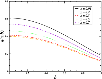
(a) (b)

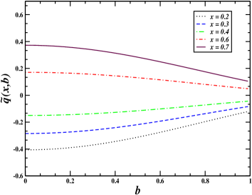
Figure 1: (Color online) Plots of impact parameter dependent pdf $q(x,b)$ and $\tilde{q}(x,b)$ vs $b$ for fixed values of $x$ where we have taken $\Lambda$ = 20 $\mathrm{GeV}$ and $\Delta_{max}$= 3 GeV where $\Delta_{max}$ is the upper limit in the $\Delta$ integration. $b$ is in ${\mathrm{GeV}}^{-1}$ and $q(x,b)$ and $\tilde{q}(x,b)$ are in ${\mathrm{GeV}}^{2}$ .

Figs 1(a) and 1(b) show the impact parameter dependent parton distributions $q(x,b)$ and $\tilde{q}(x,b)$ for unpolarized and polarized photons respectively. We took the momentum transfer to be purely in the transverse direction. We took the quark mass to be non-zero and equal to $m=m_{q}=3.3$ MeV; $\Lambda=Q=20$ GeV; $\mu=0$ and $\Delta_{max}=3.0$ GeV, where $\Delta_{max}$ is the upper limit of the Fourier transform. The smearing in $b^{\perp}$ space reveals the partonic substructure of the photon and its shape in transverse space. In the ideal definition of the Fourier transform the integration over the $\Delta^{\perp}$ should be from zero to infinity. In this case the $\Delta^{\perp}$ independent terms in the integrand would give $\delta^{2}(b^{\perp})$ in the impact parameter space. This means when there is no momentum transfer in the transverse direction, the photon behaves like a point particle in transverse position space. The distribution in transverse space is revealed only when there is non-zero momentum transfer in the transverse direction. The parton distributions for the polarized photon changes sign at $x=1/2$, at this point the GPD and the ipdpdf become zero. These parton distributions for the polarized photon are approximately symmetric about $x=1/2$ in $b$ space. For fixed $x$, $\tilde{q}(x,b)$ becomes broader as a function of $b$ as $x$ increases till $x=1/2$. For larger values of $x$, it changes sign. We have also checked that at larger values of $\Delta_{max}$ the distributions are sharper in $b$ space. The photon GPDs show qualitatively the same behaviour when the momentum transfer has both longitudinal and transverse components [10].

3 Helicity Flip Photon GPDs

In this case $\lambda^{\prime}\neq\lambda$. Our calculations show that at leading order there is only one helicity flip photon GPD. This can be expressed in terms of the two-particle LFWFs of the photon. As the photon has spin one, to flip its helicity, one of the overlapping LFWFs should have orbital angular momentum contribution of two units.

The transverse polarization vector of the photon can be written as :

$$\epsilon^{\perp}_{\pm}=\frac{1}{\sqrt{2}}(\mp 1,-i)$$ (9)

We extract the GPD that involves a helicity flip of the target photon from the non-vanishing coefficient of the combination $(\epsilon^{1}_{+1}\epsilon^{1*}_{-1}+\epsilon^{2}_{+1}\epsilon^{2*}_{-1})$. Using the overlap formula in terms of the LFWFs, the helicity flip photon GPD can be calculated and has the form [11]

$$E_{1}=\frac{\alpha e_{q}^{2}}{2\pi^{2}}x(1-x)\Big{[}I_{1}-(1-x)I_{2}\Big{]}.$$ (10)

The integrals are given by :

$$I_{1}=({(\Delta^{1})}^{2}-{(\Delta^{2})}^{2})\pi(1-x)^{2}\int_{0}^{1}dq\hskip 5.69046pt\frac{(1-q)^{2}}{B(q)};~{}~{}~{}I_{2}=({(\Delta^{1})}^{2}-{(\Delta^{2})}^{2})\pi(1-x)\int_{0}^{1}dq\hskip 5.69046pt\frac{(1-q)}{B(q)};$$ (11)

where

$$B(q)=m^{2}\Big{(}1-x(1-x)\Big{)}+q(1-q)(1-x)^{2}{(\Delta^{\perp})}^{2}.$$ (12)

$\Delta^{1}$ and $\Delta^{2}$ are the $x$ and $y$ components of $\Delta^{\perp}$ respectively.

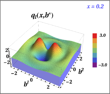
(a)    (b)

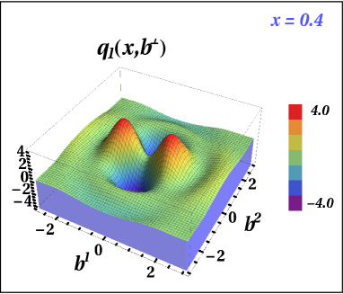
Figure 2: (Color online) Plots of $q_{1}(x,b^{\perp})$ vs $b^{1},b^{2}$ for different values of $x$ and at $\Delta_{max}=4.0$ GeV.

Similar to the GPD $E$ of a spin $1/2$ particle for example a dressed electron/quark [8], the helicity flip photon GPD has no logarithmic scale dependent term. From the expressions above, we define the parton distributions [5] with the helicity flip of the photon in transverse impact parameter space as:

$$q_{1}(x,b^{\perp})={1\over 4\pi^{2}}\int d^{2}\Delta^{\perp}e^{-i\Delta^{\perp}\cdot b^{\perp}}E_{1}(x,\Delta^{\perp});$$ (13)

where $t=-{(\Delta^{\perp})}^{2}$ and $b^{\perp}$ is the transverse impact parameter conjugate to $\Delta^{\perp}$. One obtains :

$$q_{1}(x,b^{\perp})=\frac{1}{4\pi^{2}}\int d^{2}\Delta^{\perp}e^{-ib^{\perp}\cdot\Delta^{\perp}}({(\Delta^{1})}^{2}-{(\Delta^{2})}^{2})f(x)Q(x,t),$$ (14)

where

$$f(x)=\frac{\alpha e_{q}^{2}}{2\pi}x(1-x)^{3}\hskip 14.22636pt,~{}~{}~{}~{}\hskip 14.22636ptQ(x,t)=\int_{0}^{1}\frac{dq}{B(q)}\hskip 5.69046pt((1-q)^{2}-(1-q));$$ (15)

Figs 2(a) and 2(b) show plots of the helicity flip photon GPDs in impact parameter space $q_{1}(x,b)$ vs $b_{1}$ and $b_{2}$ for a fixed value of $\Delta_{max}$ and two different values of $x$. The magnitude of the peak depends on $x$. $q_{1}(x,b)$ has a quadrupole structure, as can be seen in the plots. This structure is expected as to flip the helicity of a spin one object, one needs a LFWF with orbital angular momentum of two units.

4 Conclusion

In this talk, I have reported a recent calculation of the generalized parton distributions of the photon. Extending the calculations of [1], from the kinematics of zero $\Delta^{\perp}$ and non-zero $\zeta$, we calculated the photon GPDs for non-zero $\Delta^{\perp}$, at leading order in $\alpha$ and zeroth order in $\alpha_{s}$. The GPDs where the helicity of the photon is not flipped are logarithmically dependent on the scale. Taking the Fourier transform of the GPDs with respect to $\Delta^{\perp}$ we get the parton distributions of the photon in impact parameter space. The helicity flip photon GPDs show the expected quadrupole structure in impact parameter space.

5 Acknowledgement

This work has been done in collaboration with Sreeraj Nair and Vikash Kumar Ojha. AM thanks the organizers of the ”International Conference on the Structure and the Interactions of the Photon” for the kind invitation.

References

- [1] S. Friot, B. Pire, L. Szymanowski, Phys. Lett. B 645 153 (2007).
- [2] I. R. Gabdrakhmanov, O. V. Teryaev, Phys. Lett. B 716, 417 (2012).
- [3] W. M. Zhang, A. Harindranath, Phys. Rev. D48, 4881 (1993).
- [4] A. Mukherjee, Sreeraj Nair, Phys. Lett. B 706 77 (2011).
- [5] M. Burkardt, Int. J. Mod. Phys. A 18, 173 (2003); M. Burkardt, Phys. Rev. D 62, 071503 (2000), Erratum- ibid, D 66, 119903 (2002); J. P. Ralston and B. Pire, Phys. Rev. D 66, 111501 (2002).
- [6] S. J. Brodsky, D. Chakrabarti, A. Harindranath, A. Mukherjee and J. P. Vary, Phys. Lett. B 641, 440 (2006); Phys. Rev. D 75, 014003 (2007
- [7] D. Chakrabarti, R. Manohar, A. Mukherjee, Phys.Rev. D79, 034006,(2009).
- [8] D. Chakrabarti and A. Mukherjee, Phys.Rev.D72, 034013 (2005); Phys. Rev. D71, 014038 (2005).
- [9] D. Chakrabarti, R. Manohar, A. Mukherjee, Phys. Lett. B 682, 428 (2010); R. Manohar, A. Mukherjee, D. Chakrabarti, Phys.Rev.D83, 014004,(2011).
- [10] A. Mukherjee, Sreeraj Nair, Phys. Lett. B 707 99 (2012).
- [11] A. Mukherjee, Sreeraj Nair, Vikash Kumar Ojha, Phys. Lett. B 721 284 (2013).