Collective excitations in a large-$d$ model for graphene

Abstract

We consider a model of Dirac fermions coupled to flexural phonons to describe a graphene sheet fluctuating in dimension $2+d$. We derive the self-consistent screening equations for the quantum problem, exact in the limit of large $d$. We first treat the membrane alone, and work out the quantum to classical, and harmonic to anharmonic crossover. For the coupled electron-membrane problem we calculate the dressed two-particle propagators of the elastic and electron interactions and find that it exhibits a collective mode which becomes unstable at some wave-vector $q_{\rm c}$ for large enough coupling $g$. The saddle point analysis, exact at large $d$, indicates that this instability corresponds to spontaneous and simultaneous appearance of gaussian curvature and electron puddles. The relevance to ripples in graphene is discussed.

I introduction

Graphene is a one atom thick membrane Novoselov et al. (2004, 2005); Castro Neto et al. (2009) with a high bulk and Young elastic modulii, which can withstand large strains before fracture Lee et al. (2008). Both suspended samples and samples on substrates show corrugations on a variety of scales. In some cases these corrugations are due to inhomogeneities in the substrate Stolyarova et al. (2008); Geringer et al. (2009) (see also Viola Kusminskiy et al. (2011)), or to the mismatch between the graphene and the substrate lattice parameters de Parga et al. (2008). Freely suspended samples also show ripples, whose origin is still undetermined Meyer et al. (2007) (see also Fasolino et al. (2007)). The scale of the observed corrugations can lead to significant modifications in the electronic band structure of graphene Horovitz and  Doussal (2002); Guinea et al. (2008, 2009)).

The flexural modes of graphene are coupled to the in plane phonons, leading to anharmonic effects even in the zero temperature, quantum limit Mariani and  von Oppen (2008). Flexural modes couple to the electrons in graphene, and change the electrical conductivity Mariani and  von Oppen (2008); Castro et al. (2010); Mariani and  von Oppen (2010). Ripples might arise from the coupling between the lattice deformations and the electrons Gazit (2009a); San-Jose et al. (2011). Structural corrugations induce a shift in the electronic chemical potential, which lead to the formation of charge puddles Gibertini et al. (2012). Instabilities at finite momenta in models where the electrons are described as a perfect metal, and the formation of charge inhomogeneities is only prevented by the Coulomb interaction Gazit (2009a). On the other hand, the low density of states in graphene leads to a small quantum capacitance, although, again, a sufficiently large coupling between electrons and lattice deformations can induce instabilities San-Jose et al. (2011).

We study here the nature of the instabilities due to the combination of anharmonic effects Nelson and  Peliti (1987) and electron-phonon coupling at zero and at finite temperature. We extend the model used in San-Jose et al. (2011) by considering a membrane fluctuating in $d$ transverse dimensions and coupled to $N_{\rm f}d$ fermion species. This extension allows for an exact solution at large $d$. We derive the large $d$ equations which provide a generalization of the $1/d$ expansion Aronovitz and  Lubensky (1988); David and  Guitter (1988) and of the Self Consistent Screening Approximation (SCSA) Le Doussal and  Radzihovsky (1992) for the classical membrane to (i) the quantum membrane problem, (ii) the coupled electron-membrane quantum problem. Given the success of the SCSA to describe both classical anharmonic effects in the elastic problem Zakharchenko et al. (2010), and interaction effects in the electron problem alone (see e.g. Gonzalez et al. (1994), and confirming experiments in Elias et al. (2011)), it is indeed tempting to apply it to the coupled problem. Here we solve mainly the $d=\infty$ limit, and discuss some of the $1/d$ corrections, leaving the full study of the SCSA equations to the future. We find that as the electron-phonon coupling increases, the charge excitations become strongly hybridized with flexural phonons, and the frequencies of these excitations decrease, until a threshold is reached where an instability occurs. A saddle-point analysis, exact at large $d$, indicates that this instability corresponds to the spontaneous and simultaneous appearance of gaussian curvature and electron puddles, a hallmark of the ripples. Note that our mechanism is consistent, although different in details from San-Jose et al. (2011), since the instability occurs already for $d=\infty$ hence does not require the renormalization of the bending rigidity of the membrane. While consideration of these additional $1/d$ effects may lead to quantitative changes, it is not expected to radically alter the picture proposed here.

In addition to the coupled problem, the SCSA equations for the quantum membrane alone lead to a new “phase diagram” where we identify regions in the temperature/wave-vector plane where quantum to classical as well as harmonic to anharmonic elasticity crossovers occur, and which should be useful in analyzing experiments.

This article is organized as follows:

In section II, we introduce our model, and compare it to previous studies.

Section III introduces the equations to be solved in the self-consistent-screening method.

In Section IV we first analyze the membrane alone, and study the crossover quantum/classical and harmonic/anharmonic for the flexural modes. Then we study the coupled membrane-electron problem and present our results for the instability in section IV.

In section V, we analyze further the instability by deriving the exact effective action in the large $d$-limit.

Our conclusions are presented in section VI.

Several technical, but important details are presented in the appendices: In appendix A we discuss how to integrate over the in-plane phonons. In appendices B and C we evaluate the most important diagrams, the phonon (flexural) and fermion bubbles.

II Model

II.1 Hamiltonian of flexural phonons coupled to Dirac electrons

To consider a model with a tractable limit, we extend the model for a graphene sheet to a membrane in embedding dimension $d$, interacting with $N_{\rm f}d$ copies of a free Dirac fermion. Here $N_{\rm f}$ is the number of flavors (valleys plus spin). The physical case is recovered by setting $d=1$ and $N_{\rm f}=4$. The parameter $d$ is convenient to consider in the solvable limit $d\to\infty$. The deformation of the sheet with respect to the perfect flat crystal is parameterized by 2 in-plane phonon displacement fields $u_{i}$, $i=1,2$, and $d$ out-of-plane phonon modes $h_{a}$, $a=1,...,d$ (flexural modes). The deformation energy is the sum of curvature and elastic energy,

$$H_{\rm ph} = H_{\rm kin}+H_{\rm elas}$$ (1)

$$H_{\rm elas} = \frac{1}{2}\int\mathrm{d}^{2}x\,\Big{[}\kappa(\nabla^{2}h_{a})^{2}+\lambda u_{ii}^{2}+2\mu u_{ij}^{2}\Big{]}.$$ (2)

It is given in terms of the Lamé coefficients $\lambda,\mu$ and the strain field $u_{ij}:=\frac{1}{2}(\partial_{i}u_{j}+\partial_{j}u_{i}+\partial_{i}h_{a}\partial_{j}h_{a})$. Adding the kinetic energy $H_{\rm kin}$ leads to the quantum action which describes the membrane dynamics (in real time $t$, and with mass density $\rho$),

$${\cal S}_{\rm ph}=\int\mathrm{d}t\,\Big{\{}\mathrm{d}^{2}x\,\frac{\rho}{2}[(\partial_{t}u_{i})^{2}+(\partial_{t}h_{a})^{2}]-H_{\rm elas}\Big{\}}.$$ (3)

We now couple the long-wavelength modes of the membrane to Dirac fermions. Following previous work, we define a scalar potential, which describes a global shift of the chemical potential, and a gauge field, which describes the hopping between the two sublattices which make up graphene Vozmediano et al. (2010). The scalar potential modifies the local chemical potential, and induces charge fluctuations. The change in the electronic energy associated to charge fluctuations is described, in second order perturbation theory, by the charge susceptibility, $\chi_{\rho}(q,\omega)=\sum_{n}\left|\left<0|\hat{\rho}_{q})|n\right>\right|^{2}\delta(\omega-\epsilon_{n}+\epsilon_{0})$ where $\hat{\rho}_{q}$ creates an electron-hole pair of momentum $q$, $\left|0\right>$ and $\left|n\right>$ are the ground and excited states, and $\epsilon_{0}$ and $\epsilon_{n}$ their energies. The gauge potential, on the other hand, couples to the current operator, and it induces current fluctuations. The term which describes the effect of these fluctuations on the total energy is given by the current susceptibility, $\chi_{j}(q,\omega)$, which is related to the charge susceptibility by charge conservation $\chi_{j}(q,\omega)=\omega^{2}/(v_{F}^{2}q^{2})\times\chi_{\rho}(q,\omega)$. As, for flexural modes, $\omega_{\rm fl}(q)\propto q^{2}\ll v_{F}q$ over the entire Brillouin Zone, and we can neglect the contribution of the gauge potential as $q\rightarrow 0$ San-Jose et al. (2011).

In this article we consider the coupling to a scalar potential, modeled by

$$H_{\rm e\text{-}ph} = -g_{0}\int\mathrm{d}^{2}x\,\delta\rho(x)u_{ii}(x)$$ (4)

$$\delta\rho(x) = \rho(x)-\rho_{0}=\frac{1}{d}\sum_{\gamma=1}^{N_{\rm f}d}\bar{\Psi}_{\gamma}1{\rm l}\Psi_{\gamma}-\rho_{0}\quad$$ (5)

which is the standard form of the long-wavelength coupling assuming (i) rotational invariance, i.e. no substrate, (ii) no membrane tension (arising from e.g.  clamping)– it can be added later. Here $\rho_{0}$ is the equilibrium carrier density counted from the neutrality point. Estimations for the value of $g_{0}$ vary over one order of magnitude Ono and  Sugihara (1966); Suzuura and  Ando (2002); Choi et al. (2010), $g_{0}\approx 4-50$ eV.

In previous work Gazit (2009a); San-Jose et al. (2011) the strategy was to first integrate over fermions (within some approximation, see below) and only in a second stage sum over in-plane modes, to obtain an effective (approximate) theory for the flexural modes only. Our present strategy is different. We first integrate over in-plane phonons leading to a coupled theory of flexural modes and electrons. Since the action is quadratic in these modes, the integration can be performed exactly. The calculation is performed in details in Appendix A. Because of the frequency dependence of the in-plane phonon propagator we obtain a more complicated expression than in the standard (i.e. classical) case. It contains new, frequency dependent, terms. Since in this article we focus on frequencies of the order of the Debye frequencies of flexural modes, which are much lower than the one for in-plane phonons, this new frequency dependence can safely be neglected. Hence we arrive at our starting (effective) Hamiltonian for the flexural modes coupled to the free Dirac electrons (we set $\hbar=1$):

$$H=H_{\rm kin} + H_{\rho}+\int\mathrm{d}^{2}x\bigg{\{}\sum_{a=1}^{d}\frac{\kappa}{2}(\nabla^{2}h_{a})^{2}$$ (6)

$$+\frac{K_{0}}{2d}\bigg{[}\frac{1}{2}{\rm P}^{\rm T}_{ij}(\partial)\sum_{a=1}^{d}\partial_{i}h_{a}\partial_{j}h_{a}\bigg{]}^{2}$$

$$-\frac{g}{d}\sum_{\gamma=1}^{N_{\rm f}d}\bar{\Psi}_{\gamma}1{\rm l}\Psi_{\gamma}\bigg{[}\frac{1}{2}{\rm P}^{\rm T}_{ij}(\partial)\sum_{a=1}^{d}\partial_{i}h_{a}\partial_{j}h_{a}\bigg{]}$$

$$+\sum_{\gamma=1}^{N_{\rm f}d}\bar{\Psi}_{\gamma}\big{[}-v_{\rm F}{{\boldsymbol{\sigma}}}\cdot(-i\nabla)\big{]}\Psi_{\gamma}\bigg{\}}.$$

Here $K_{0}=4\mu(\mu+\lambda)/(2\mu+\lambda)d$ is the bare Young modulus, to which should be added the kinetic energy. Note that the resulting coupling becomes

$$g=\frac{2\mu}{2\mu+\lambda}g_{0}.$$ (7)

In graphene, $\lambda/\mu\approx 1/6$, so that $g\approx g_{0}$.

In a second stage (see below) we will add to this model the electron-electron interaction. The energy for the charge fluctuations then take the form:

$$H_{\rm ee}=\frac{1}{2}\int\frac{\mathrm{d}^{2}q}{(2\pi)^{2}}V_{0}(q)|\rho(q)|^{2}.$$ (8)

We consider below the Coulomb interaction $V_{0}(r)=e^{2}/(\epsilon_{0}r)$, i.e. in Fourier $V_{0}(q)=\frac{2\pi e^{2}}{\epsilon_{0}q}$, where $\epsilon_{0}$ is the dielectric constant of the environment. This term $H_{ee}$ will be added to (6).

After integration over the in-plane phonons the interaction becomes

$$V(q)=V_{0}(q)-\frac{g_{0}^{2}}{\lambda+2\mu}.$$ (9)

i.e. it acquires a short-ranged attractive part, as shown in Appendix A. By power counting that part is formally irrelevant and can be neglected at small $q$ compared to the Coulomb repulsion . At higher $q$ however, and especially if a ripple instability develops, it does play a role and may not be neglected. This will be discussed below and in Section IV.2.

Finally, note that in the elastic interaction the uniform mode is excluded, i.e. everywhere in this article the composite field ${\rm P}^{\rm T}_{ij}(\partial)\sum_{a=1}^{d}\partial_{i}h_{a}\partial_{j}h_{a}$ is evaluated only for Fourier components $q\neq 0$ Nelson et al. (1989); Le Doussal and  Radzihovsky (1992); WieseHabil . This field, which plays an important role below, has a nice geometrical interpretation, i.e. it is equal (say for $d=1$), in Fourier, to ${\cal K}(q)/q^{2}$ where ${\cal K}(x)$ is the Gaussian curvature of the membrane.

II.2 Comparison with previous work

Let us contrast again our approach with previous work Gazit (2009a); San-Jose et al. (2011). There one first integrated the coupling term (4) over the electrons using a Gaussian approximation. There the degree of freedom are the charge fluctuations $\delta\rho$, and one replaces the electronic part of the Hamiltonian with:

$$H_{\rm\rho} = \frac{1}{2}\int\mathrm{d}^{2}q\,|\delta\rho(q)|^{2}\left[\frac{1}{\chi_{\rho}(q)}+V_{0}(q)\right]$$ (10)

As the term in eq.(10) is quadratic, it can be combined with eq.(4) and the charge fluctuations can be integrated out leading to an additional term in the elastic energy which could be interpreted as a $q$-dependent shift in the Lame coefficient:

$$\lambda\to\lambda(q)=\lambda-g_{0}^{2}\langle\delta\rho(-q)\delta\rho(q)\rangle.$$ (11)

In this calculation, the electron-density correlation was estimated either from a fluid model for the interacting electrons Gazit (2009a) (a finite-$T$ classical calculation using $H_{\rho}$ without the first term), or from the susceptibility $\chi_{\rho}(q)$ of non-interacting Dirac fermions San-Jose et al. (2011) (a $T=0$ quantum calculation, using $H_{\rho}$ including the first term).

In a second stage one integrated over the in-plane modes, resulting in the usual membrane action, but with a modified, wave-vector dependent, Young’s modulus $K_{0}(q)=\frac{4\mu[\mu+\lambda(q)]}{2\mu+\lambda(q)}$. In the classical fluid estimate Gazit (2009a), one finds $\lambda\to\lambda-g^{2}q/(2\pi e^{2})$ and $K_{0}(q)$ changes sign in some (relatively narrow) region of momenta $\frac{2\pi e^{2}}{g^{2}}(2\mu+\lambda)>q>\frac{2\pi e^{2}}{g^{2}}(\mu+\lambda)$. Using the standard SCSA method for classical membranes to treat the effect of $K_{0}(q)$, this was then argued to lead to a maximum in the normal-normal correlation of the membrane, interpreted as ripples. In San-Jose et al. (2011) the renormalization of the wave-vector dependent bending rigidity $\kappa(q)$, resulting from this dispersive Young modulus was estimated in the quantum $T=0$ limit, and argued to lead to two different regimes. In one regime $\kappa(q)$ softens near a finite $q$, which was argued to lead to ripples at that wave-vector. Note that other proposals, based on buckling, also exist in the literature Guinea et al. (2008); Brey and  Palacios (2008); Gazit (2009b).

While it is tempting to first integrate over the Dirac fermions, it is in practice difficult to do it accurately, beyond the classical-fluid approximation. Even for non-interacting Dirac fermions, an exact calculation leads to a functional determinant and higher non-linearities in $u_{ii}$. In addition, as we will see, it may obscure one piece of the physics, which is that the instability that we seek to describe is a combined instability in flexural modes and electron density. Furthermore, interactions are easily seen to stabilize the system, hence we need to include them for any realistic theory, which makes integration over fermions in a first step even more problematic.

Hence we choose a different route and first integrate over in-plane modes, a step which is well controlled. The resulting theory (6) is quartic in both flexural modes and electrons, and quite non-trivial. We then solve this theory in the large-$d$ limit. The instability occurs in a different manner as in previous work, namely as a pole in the combined 2-particle propagators for phonons and electrons. In particular, we do not need to consider the renormalization of $\kappa$ to obtain a transition. Although the bending rigidity is corrected to higher orders in our $1/d$ expansion, it may change estimates for the numbers, but not the general scenario, which is a phase transition. Note that we can recover in our model $K_{0}(q)$ obtained by the previous methods (see Section IV.2); it does not seem to play an important role.

II.3 The parameters of the model

Before we analyze the model, let us recall the dimensions of the parameters (in units of length $L$ and energy $E$) and provide some estimates. The model is described by the parameters $K_{0}\equiv EL^{-2},\kappa\equiv E,\rho^{-1}=EL^{4},v_{\rm F}\equiv EL,e^{2}\equiv EL,g\equiv E$, and the momentum cutoff $\Lambda\equiv L^{-1}$ (and time $t\sim E^{-1}$). By multiplying the parameters which describe the interactions, $K_{0},e^{2}$ and $g$, with the susceptibilities, three dimensionless coupling constants can be defined

$$\lambda_{\rm anh}:=\frac{K_{0}}{\kappa^{3/2}\rho^{1/2}}\quad,\quad\alpha_{\rm e}:=\frac{e^{2}}{v_{\rm F}}$$ (12)

$$\lambda_{\rm e\text{-}fl}:=\frac{g}{\sqrt{\kappa^{3/2}\rho^{1/2}v_{\rm F}/\Lambda}}.$$

The parameter $\alpha_{\rm e}$ is the fine structure constant of graphene and characterizes the strength of the electron-electron interaction. The coupling $\lambda_{\rm anh}$ characterizes the strength of the anharmonic elasticity. The dependence of $\lambda_{\rm e\text{-}fl}$ on the cutoff $\Lambda$ shows that the electron-flexural phonon coupling is irrelevant at large distance, while the two other couplings are marginal. This analysis applies to the quantum, low temperature, regime. In the classical regime (higher temperatures) there is a single coupling constant (which does not contain $\rho$), given by

$$\lambda_{\rm cl}=\frac{\lambda_{\rm e\text{-}fl}}{\sqrt{\lambda_{\rm anh}}}=\frac{g}{\sqrt{K_{0}v_{\rm F}/\Lambda}}.$$ (13)

It measures the strength of the coupling and is again irrelevant at large scale.

Numerical estimates of the parameters appearing in Eq. (12) are Castro Neto et al. (2009)

$$a=1.4{\rm\AA},\qquad a^{2}K_{0}\approx 20{\rm eV},\qquad\kappa\approx 1{\rm eV}$$

$$\Lambda_{{\rm c},h}\sim\pi/a,\qquad a^{4}\rho=M_{C}a^{2}=1/E_{C}\approx 1/(10^{-3}{\rm eV})$$

$$\omega_{{\rm c},h}\approx\sqrt{\frac{\kappa}{\rho}}\Lambda_{\rm c,h}^{2}\approx\sqrt{10^{-3}}{\rm eV},$$

$$\frac{v_{\rm F}}{a}\approx 5{\rm eV},\qquad\alpha_{\rm e}=\frac{e^{2}}{\epsilon_{0}v_{\rm F}}\approx 2$$ (14)

where $\epsilon_{0}$ is the dielectric constant of the environment. The value above is obtained for suspended samples, $\epsilon_{0}=1$. The parameter $\Lambda_{{\rm c},h}$ gives the UV-cutoff for the $h$ field, and $\omega_{{\rm c,h}}$ is the corresponding frequency.

With these values of the parameters, the dimensionless couplings defined above are all of order unity $\lambda_{\rm anh}\approx 0.6,\alpha_{\rm e}\approx 2$ and $\lambda_{\rm e\text{-}fl}\approx 0.6-7$. The value of the last parameter is subject to a significant uncertainty, since, as mentioned above, estimates for $g_{0}\approx g$ can vary by one order of magnitude. The ensuing probable range for the classical coupling constant is $\lambda_{\rm cl}\approx g/5.6\approx 0.7-8.8$.

At finite temperature the flexural-phonon propagator is modified by the inclusion of the Bose-Einstein distribution, which tends to the Boltzmann distribution at temperatures higher than the phonon frequencies. Fluctuations are enhanced as the temperature increases, making the anharmonic effects discussed here more important. A detailed analysis is carried out in Section IV.1.

III self-consistent screening method

We now give the complete SCSA equations in the Matsubara equilibrium setting. They are much more general than what we will be able to achieve below, but we hope they can stimulate further studies.

III.1 Matsubara partition sum

The equilibrium Matsubara partition sum is $Z=\int{\cal D}[h]{\cal D}[\Psi]{\cal D}[\bar{\Psi}]e^{-S}$ in terms of the imaginary-time Matsubara action $S=S_{0}+S_{\rm int}$ with

$$S_{0} = \int\mathrm{d}^{2}x\int_{0}^{\beta}\mathrm{d}\tau\,\sum_{a=1}^{d}\bigg{[}\frac{\rho}{2}(\partial_{\tau}h_{a})^{2}+\frac{\kappa}{2}(\nabla^{2}h_{a})^{2}\bigg{]}+\frac{1}{\beta}\sum_{\omega^{\prime}_{n}}\int_{q}\sum_{\gamma=1}^{N_{\rm f}d}\bar{\Psi}_{\gamma}(-q,-\omega^{\prime}_{n})\bigg{[}-v_{\rm F}\boldsymbol{\sigma}\cdot(-i\nabla)-(i\omega^{\prime}_{n}+\mu)1{\rm l}\bigg{]}\Psi_{\gamma}(q,\omega^{\prime}_{n})$$

$$S_{\rm int} = \frac{1}{d}\frac{1}{\beta}\sum_{\omega_{n}}\int_{q}\Bigg{\{}\frac{1}{2}\bigg{[}\frac{1}{2}{\rm P}^{\rm T}_{ij}(\partial)\sum_{a=1}^{d}\partial_{i}h_{a}\partial_{j}h_{a}\bigg{]}_{q,\omega_{n}}K_{0}(q,\omega_{n})\bigg{[}\frac{1}{2}{\rm P}^{\rm T}_{ij}(\partial)\sum_{a=1}^{d}\partial_{i}h_{a}\partial_{j}h_{a}\bigg{]}_{-q,-\omega_{n}}$$

$$-\sum_{\gamma=1}^{N_{\rm f}d}[\bar{\Psi}_{\gamma}1{\rm l}\Psi_{\gamma}]_{-q,-\omega_{n}}g(q,\omega_{n})\left[\frac{1}{2}{\rm P}^{\rm T}_{ij}(\partial)\sum_{a=1}^{d}\partial_{i}h_{a}\partial_{j}h_{a}\right]_{q,\omega_{n}}+\frac{1}{2}\sum_{\gamma=1}^{N_{\rm f}d}\left[\bar{\Psi}_{\gamma}1{\rm l}\Psi_{\gamma}\right]_{q,\omega_{n}}V(q,\omega_{n})\sum_{\gamma=1}^{N_{\rm f}d}\left[\bar{\Psi}_{\gamma}1{\rm l}\Psi_{\gamma}\right]_{-q,-\omega_{n}}\Bigg{\}}.$$

We have enlarged the model to frequency and momentum dependent couplings for future convenience. The bare couplings are $K_{0}(q,\omega)=K_{0}$, $g(q,\omega)=g$. The bare electron-electron interaction is $V(q,\omega)=V(q)$. We denote by $\tau$ the imaginary time, and by $\omega_{n}:=2\pi n/\beta$ the bosonic Matsubara frequencies. The fermionic ones are $\omega^{\prime}_{n}:=2\pi(n+\frac{1}{2})/\beta$; we will need them only rarely, since the composite fields $\bar{\Psi}_{a}1{\rm l}\Psi_{a}$, as well as the polarization bubble (denoted $J$ below), contain only bosonic frequencies. We have added a chemical potential $\mu$ for the electrons, but we will set it to zero in the following. We denote $\int_{q}:=\int_{|q|<\Lambda}\frac{\mathrm{d}^{2}q}{(2\pi)^{2}}$ with an implicit UV cutoff $\Lambda$. The Pauli matrices are denoted in bold face, $\boldsymbol{\sigma}_{x}:=\left({0\atop 1}{1\atop 0}\right)$, $\boldsymbol{\sigma}_{y}:=\left({0\atop-i}{i\atop 0}\right)$, to not confuse them with the auxiliary field $\sigma$ to be introduced later. By $q\cdot\boldsymbol{\sigma}$ we denote the matrix $q_{x}\boldsymbol{\sigma}_{x}+q_{y}\boldsymbol{\sigma}_{y}$.

III.2 Bare propagators: Quantum and classical limits

In the absence of interactions, the bare propagators of the flexural phonon and of the free fermions are obtained from $S_{0}$ as

$$\langle h_{a}(-q,-\omega_{n})h_{b}(q,\omega_{n})\rangle_{0}=\delta_{ab}G(q,\omega_{n}),$$ (16)

$$G(q,\omega_{n})=\frac{1}{\kappa q^{4}+\rho\omega_{n}^{2}}$$ (17)

$$\langle\bar{\Psi}_{\gamma}(-q,-\omega^{\prime}_{n})\Psi_{\beta}(q,\omega^{\prime}_{n})\rangle=F_{\gamma\beta}(q,\omega^{\prime}_{n})\qquad$$ (18)

$$F(q,\omega^{\prime}_{n})=(i\omega^{\prime}_{n}1{\rm l}+v_{\rm F}q\cdot{\boldsymbol{\sigma}})^{-1}$$

$$\qquad~{}~{}~{}~{}~{}=-\frac{1}{v_{\rm F}^{2}q^{2}+{\omega^{\prime}_{n}}^{2}}(i\omega^{\prime}_{n}1{\rm l}-v_{\rm F}q\cdot\boldsymbol{\sigma}).$$ (19)

We recall that real-time equilibrium response functions are recovered from these propagators via the analytical continuation $i\omega_{n}\to\omega+i\delta$ and $\delta=0^{+}$. For instance the equal-time equilibrium correlation function in real time is obtained from the fluctuation-dissipation theorem (FDT) as (restoring the $\hbar$ factors)

$$C(q) := \frac{1}{d}\langle h^{a}_{q,t}h^{a}_{q,t}\rangle$$ (20)

$$= \int\frac{\mathrm{d}\,\omega}{2\pi}\hbar\coth\!\left(\frac{\beta\hbar\omega}{2}\right){\rm Im\!}\left(\frac{1}{\kappa q^{4}-\rho\omega^{2}-i\delta\omega}\right)$$

$$= \frac{\hbar\coth\!\big{(}\frac{\beta\hbar\omega_{\rm fl}(q)}{2}\big{)}}{2\rho\omega_{\rm fl}(q)}.$$

Here $\omega_{\rm fl}(q)=q^{2}\sqrt{\kappa/\rho}$ is the frequency of the flexural phonons. Eq. (21) interpolates between $C(q)=\frac{\hbar}{2\rho\omega_{\rm fl}(q)}$ in the quantum (i.e. zero-temperature) limit, to $C(q)=T/\kappa q^{4}$ in the classical (i.e. high-temperature) limit. The same result is obtained from the imaginary-time, equal-time average by performing the Matsubara summation

$$C(q)=\frac{1}{\beta}\sum_{\omega_{n}}G(q,\omega_{n})\stackrel{{\scriptstyle\beta\to 0}}{{\longrightarrow}}\frac{1}{\beta}G(q,\omega_{n}=0)=\frac{T}{\kappa q^{4}}\ .$$ (21)

In the high-temperature limit, $\beta\to 0,$ one can replace $G(q,\omega_{n})\to\delta_{n0}\frac{1}{\kappa q^{4}}$, hence only the mode $\omega_{n}=0$ contributes, and (21) reproduces the classical result. This remark will be important to recover the classical SCSA equations from the quantum ones below.

III.3 SCSA equations

As is well-known from the $O(N)$ model (here $N\equiv d$) for $d=\infty,$ one can calculate exactly the dressed quartic interactions as a geometric sum of the polarization bubbles. In these bubbles one uses the bare propagators, $G$ for the phonons and $F$ for the fermions, which will be mainly what we achieve to do explicitly here. However, one can aim to go further and also calculate the corrections to the self-energies to first order in $1/d$, leading to the dressed propagators denoted $\tilde{G}$ and $\tilde{F}$. The SCSA equations are the coupled Dyson equations which determine both the dressed propagators and the dressed interactions. They provide a self-consistent approximation for any $d$. If one uses the bare propagators in these equations (as done below), they give the dominant order at large $d$ for the interaction and the self-energy. Hence they are exact at large $d$ to dominant order in $1/d$.

One starts by defining the (dressed) phonon bubble and (dressed) fermion loop as

$$I(q,\omega) = \frac{1}{\beta}\sum_{\Omega_{n}}\int_{p}[p\cdot{\rm P}^{\rm T}(q)\cdot p]^{2}\tilde{G}(p,\Omega_{n})$$ (22)

$$\qquad~{}~{}~{}~{}~{}\times\tilde{G}(p+q,\omega+\Omega_{n})$$

$$J(q,\omega) = -\frac{1}{\beta}\sum_{\Omega^{\prime}_{n}}\int_{p}\mathrm{tr}\Big{(}\tilde{F}(p,\Omega^{\prime}_{n})\tilde{F}(p+q,\omega+\Omega^{\prime}_{n})\Big{)}\qquad$$ (23)

They are given in terms of the (dressed) propagators. Everywhere in this Section we work in Matsubara time, hence $\omega$ designates everywhere $\omega_{n}$ (or $\omega^{\prime}_{n}$ for fermions), thus $I(q,\omega)$ and $J(q,\omega)$ are not defined for all $\omega$, but only the quantized, bosonic Matsubara frequencies. The same equations also hold in real time, substituting $\omega\to-i\omega+\delta$.

III.3.1 Decoupled problem: Membrane

In the absence of a coupling between electrons and phonons, we can consider separately the membrane and the electron problem. The flexural propagator, including the correction to the self-energy of the flexural modes due to the quartic interaction, reads

$$\tilde{G}(q,\omega)^{-1} = \kappa q^{4}+\rho\omega^{2}$$ (24)

$$+\frac{1}{d}\frac{1}{\beta}\sum_{\Omega_{n}}\int_{p}[q\cdot{\rm P}^{\rm T}(p)\cdot q]^{2}\tilde{K}_{0}(p,\Omega_{n})$$

$$\qquad~{}~{}~{}~{}~{}~{}~{}~{}\times\tilde{G}(p+q,\omega+\Omega_{n}).$$

It is given in terms of the dressed interaction,

$$\tilde{K}_{0}(q,\omega)=\frac{K_{0}}{1+\frac{1}{2}K_{0}I(q,\omega)}.$$ (25)

Equations (22), (24) and (25) define the (quantum) SCSA equations for the membrane, i.e. for the phonon problem alone.

In the high-temperature limit $\beta\to 0$, as discussed above, $\tilde{G}(q,\omega_{n})=\delta_{n0}\tilde{G}(q)$, $\tilde{K}_{0}(q,\omega_{n})=\delta_{n0}\tilde{K}_{0}(q)$, $I(q,\omega_{n})=\delta_{n0}I(q)$, and the above equations reduce to the classical SCSA equations of Ref.  Le Doussal and  Radzihovsky (1992) (with the correspondence from here to there $K_{0}\to 2b$, $I\to 3I$, $T\to 1$). As is well known, the self-consistent solution of these equations at small $q$ leads to: (i) the softening of the elastic modulii $\tilde{K}_{0}(q)\sim q^{\eta_{u}}$ due to the screening of the elastic interactions by thermally excited out-of-plane modes, (ii) a stiffening of the bending rigidity $\tilde{G}(q)\sim q^{4-\eta}$ (equivalently $\kappa(q)\sim q^{-\eta}$) with $\eta=4/(d+\sqrt{16-2d+d^{2}})$, $\eta_{u}=2-2\eta$, i.e. in $d=1$, $\eta\approx 0.82$, $\eta_{u}\approx 0.36$ in good agreement with first-principle numerical studies of graphene sheets Zakharchenko et al. (2010). While the SCSA provides a reasonable approximation for any $d$, to obtain the direct-expansion result $\eta=2/d+O(1/d^{2})$ and $\eta_{u}=2+O(1/d),$ it is sufficient to use the bare propagator $\tilde{G}(q)\to G(q)$ in all integrals of the SCSA equations. Note that more recently the SCSA has been extended to the next order in $1/d$ Gazit (2009c).

III.3.2 Decoupled problem: Dirac electrons

Consider now the SCSA equations for the electrons alone, in presence of a bare electron-electron interaction $V(q)$. The correction to the self-energy of the electrons due to the quartic electron-electron interaction reads

$$\tilde{F}(q,\omega)^{-1} = v_{\rm F}q\cdot\boldsymbol{\sigma}+i\omega$$ (26)

$$+\frac{1}{d\beta}\sum_{\Omega_{n}}\int_{p}\tilde{V}(p,\Omega_{n})\tilde{F}(p+q,\omega+\Omega_{n}).~{}~{}~{}~{}~{}~{}~{}$$

$\tilde{V}$ is the dressed interaction,

$$\tilde{V}(q,\omega)=\frac{V(q)}{1+N_{\rm f}V(q)J(q,\omega)}.$$ (27)

Equations (23), (26) and (27) are the SCSA equations for the electron problem alone. If the bare propagators are inserted, these equations are called GW and RPA and have been studied Gonzalez et al. (1994) for the Coulomb interactions at $T=0$. They exhibit a logarithmic divergence; thus the corresponding RG flow for $v_{\rm F}$ and the wave-function renormalization $Z$ was obtained, implicitly, to first order in $1/(dN_{\rm f})$. In the infrared $v_{\rm F}$ increases, leading to a downward flow of the dimensionless coupling $\alpha_{\rm e}$ (since $e^{2}$ is not renormalized), which is marginally irrelevant Gonzalez et al. (1994). This effect was observed in experiments Elias et al. (2011).

III.3.3 Coupled problems

Since the SCSA has been so successful to describe separately the membrane and the electron problem, it is tempting to apply it to the coupled problem.

In the presence of an electron-phonon coupling, the bubbles $I$ and $J$ are still defined by (22) and (23), and the equations (24) and (26) are still valid. To express the dressed interactions however, we must now consider 2 by 2 matrices. We define (for each $q$ and $\omega$, which are implicit),

$$\tilde{\cal V} := \left(\begin{array}[]{cc}\tilde{K}_{0}&-\tilde{g}\\ -\tilde{g}&\tilde{V}\end{array}\right),$$ (30)

$${\cal V} := \left(\begin{array}[]{cc}K_{0}&-g\\ -g&V\end{array}\right),$$ (33)

$${\cal J} := \left(\begin{array}[]{cc}\frac{1}{2}I&0\\ 0&N_{\rm f}J\end{array}\right).$$ (36)

The last SCSA equation expresses the dressed interactions as

$$\tilde{\cal V}={\cal V}(1{\rm l}+{\cal J}{\cal V})^{-1}.$$ (37)

The matrix elements are

$$\tilde{K}_{0}(q,\omega) = \frac{K_{0}[1+N_{\rm f}V(q)J(q,\omega)]-g^{2}N_{\rm f}J(q,\omega)}{D(q,\omega)},~{}~{}~{}~{}~{}~{}~{}$$ (38)

$$\tilde{g}(q,\omega) = \frac{g}{D(q,\omega)},$$ (39)

$$\tilde{V}(q,\omega) = \frac{V(q)[1+\frac{1}{2}K_{0}I(q,\omega)]-\frac{1}{2}g^{2}I(q,\omega)}{D(q,\omega)}.$$ (40)

We have defined the determinant

$$D={\rm det}(1{\rm l}+{\cal J}{\cal V}).$$ (41)

More precisely,

$$D(q,\omega) = \Big{[}1+\frac{1}{2}K_{0}I(q,\omega)\Big{]}\Big{[}1+N_{\rm f}V(q)J(q,\omega)\Big{]}$$ (42)

$$-\frac{N_{\rm f}}{2}g^{2}I(q,\omega)J(q,\omega).$$

The closed set of equations (22), (23), (24), (26), and (38)–(42) are the SCSA equations for the coupled electron-phonon problem. Again, they are exact at dominant order for $d\to\infty$ (in which case we can use bare propagators in the integrals). Alternatively, using the dressed propagators, they provide an approximation for any $d$. They also contain the two special cases of the uncoupled systems discussed above.

It is important to note the equivalent formulation in terms of “dressed bubbles”, or dressed two-particle propagators, or susceptibilities as

$$\tilde{\cal J} = (1{\rm l}+{\cal J}{\cal V})^{-1}{\cal J}={\cal J}(1{\rm l}+{\cal V}{\cal J})^{-1},$$ (43)

$$\tilde{\cal J} = \left(\begin{array}[]{cc}\frac{1}{2}\tilde{I}&\tilde{\Pi}\\ ~{}\tilde{\Pi}&N_{\rm f}\tilde{J}\end{array}\right).$$ (46)

It satisfies $\tilde{\cal V}={\cal V}-{\cal V}\tilde{\cal J}{\cal V}$ and $\tilde{\cal J}={\cal J}-{\cal J}{\cal V}\tilde{\cal J}$, more specifically,

$$\tilde{I}(q,\omega) = I(q,\omega)\Big{[}1+N_{\rm f}V(q)J(q,\omega)\Big{]}/D(q,\omega)\qquad$$ (47)

$$\tilde{\Pi}(q,\omega) = \frac{1}{2}gN_{\rm f}I(q,\omega)J(q,\omega)/D(q,\omega)$$ (48)

$$\tilde{J}(q,\omega) = J(q,\omega)\Big{[}1+\frac{1}{2}K_{0}I(q,\omega)\Big{]}/D(q,\omega)$$ (49)

The interest of this approach is that if one calls the composite fields,

$$\Phi(x)=\frac{1}{d}\sum_{a}\frac{1}{2}{\rm P}^{\rm T}_{ij}(\partial)\partial_{i}h^{a}(x)\partial_{j}h^{a}(x)$$ (50)

$$\rho(x)=\frac{1}{d}\sum_{\gamma=1}^{N_{\rm f}d}\bar{\Psi}_{\gamma}(x)1{\rm l}\Psi_{\gamma}(x)-\rho_{0}$$ (51)

Then

$$\tilde{\cal J}=d\left(\begin{array}[]{cc}\langle\Phi(-q,-\omega)\Phi(q,\omega))\rangle&\langle\Phi(-q,-\omega)\rho(q,\omega)\rangle\\ \langle\rho(-q,-\omega)\Phi(q,\omega))\rangle&\langle\rho(-q,-\omega)\rho(q,\omega)\rangle\end{array}\right).$$ (52)

We will not attempt to solve here the self-consistent equations (22), (23), (24), (26), and (38)–(42). Instead we will use them by inserting the bare propagators $\tilde{G}\to G$ and $\tilde{F}\to F$ in all the integrals in the SCSA equations. Then to leading order in $d\to\infty$ we need only (22), (23) and (38)–(42). The additional equations (24), (26) then give the $O(1/d)$ corrections to the propagators. These lead to the renormalizations of $\kappa,\rho,\alpha_{e},v_{\rm F}$ which we will not study in detail here, as they are not needed to leading order at large $d$.

IV Analysis of the results

We start by giving the explicit expression for the bubbles $I$ and $J$, calculated with the bare propagators, hence denoted below $I_{0}$ and $J_{0}$. Then we analyze the consequences first for the membrane alone, and then for the coupled system.

IV.1 Flexural bubble and membrane alone

A general expression for the flexural bubble $I_{0}$ at any temperature is given in Appendix B. An explicit form is obtained in the quantum limit, $T=0,$ and in the classical limit. The result there is given in Matsubara frequency.

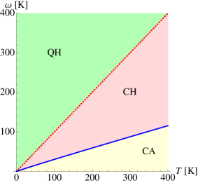
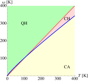
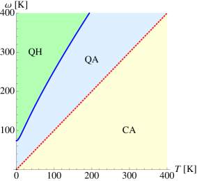
Figure 1: Crossovers in scales: plot of $\omega_{a}(T)$ versus $T$ (both in Kelvin) for $\lambda_{\rm anh}=5,16,35$ (from top left to bottom) corresponding to the three regimes (i-iii) described in the text. The diagonal $\omega_{a}=T$ divides quantum from classical region. Four combined regions are possible, as represented (QH: quantum-harmonic, QA: quantum-anharmonic,CH: classical-harmonic,CA: classical-anharmonic). The vertical axis equivalently measures the wavector squared $q_{\rm anh}^{2}=\frac{\omega_{a}}{100K}\times 0.14$ Å^-2 For simplicity the approximation $g(x)\approx 1/(1+5x)$ is used, which is found to be accurate.

IV.1.1 Zero frequency and zero temperature (quantum) limit:

Let us start with the result at zero frequency (which is the same in real and imaginary time). In the quantum case the momentum integral is UV divergent and depends on the UV cutoff $\Lambda$. At $T=0$ it reads, in dimensionless form,

$$K_{0}I_{0}(q,0) = \frac{3}{64\pi}\lambda_{\rm anh}f(s),$$ (53)

$$f(s) = \frac{2}{3(s+1)}+\frac{1}{2}\log\left(\frac{s+1}{16}\right)+\frac{3}{4},\qquad$$ (54)

$$s = \frac{4\Lambda^{2}}{q^{2}}.$$ (55)

The parameter $\lambda_{\rm anh}$ was defined in (12). The function $f(s)$ is of order unity, and we have given its explicit form for the circular cutoff used, see Appendix B. Let us stress that its details depend on the chosen cutoff. However, $I_{0}(q,0)$ is a log-divergent integral, and its dependence on $\ln\Lambda/(2p)$ is universal, which can be summarized by a RG equation at $T=0$,

$$-\frac{q\partial}{\partial{q}}I_{0}(p,0)=\frac{\Lambda\partial}{\partial\Lambda}I_{0}(q,0)=\frac{3}{64\pi\kappa^{3/2}\sqrt{\rho}},\mbox{ for }q\ll\Lambda.$$ (56)

For $d=\infty$, inserting the form of $I_{0}(q,0)$ in (25), we obtain the effective Young modulus $\tilde{K}_{0}:=\tilde{K}_{0}(q,0)$ at momentum $q$. It satisfies the exact RG equation (valid at all $T$) obtained from (25),

$$-q\partial_{q}\tilde{K}_{0}(q,0)=-\frac{1}{2}\Big{[}-q\partial_{q}I_{0}(q,0)\Big{]}\tilde{K}_{0}^{2}(q,0).$$ (57)

Using (56) it yields the RG equation in the quantum limit $T=0$ as

$$-\frac{q\partial}{\partial{q}}\tilde{K}_{0}(q,0)=-\frac{3}{128\pi\kappa^{3/2}\sqrt{\rho}}\tilde{K}_{0}^{2}(q,0),\ T=0,\ q\ll\Lambda,$$ (58)

recovering the result of Ref. San-Jose et al. (2011).

To estimate the importance of the anharmonic effects, let us write schematically the relative correction to the Young modulus at any $T$ as

$$-\frac{\delta K_{0}}{K_{0}}=-\frac{\tilde{K}(q,0)-K_{0}}{K_{0}}\approx\frac{1}{2}K_{0}I_{0}(q,0),$$ (59)

and define the anharmonic scale by the wave-vector $q_{\rm anh}(T)$ such that

$$\left|\frac{\delta K_{0}}{K_{0}}\right|\approx 1/2\quad,\quad K_{0}I_{0}(q_{\rm anh},0)\approx 1\ .$$ (60)

It means that above this length scale, i.e. for $q<q_{\rm anh}(T)$, the anharmonic effects are important, while for smaller length scales the corrections to the bare elastic energy due to the quartic $h$ vertex can be neglected, a regime which we call “harmonic”.

Our result at $T=0$ is thus:

$$-\frac{\delta K_{0}}{K_{0}}\approx\frac{3\lambda_{\rm anh}}{128\pi}\ln\left(\frac{2e^{3/4}\Lambda}{q}\right)$$ (61)

$$q_{\rm anh}(T=0)\approx\Lambda e^{-\frac{64\pi}{3\lambda_{\rm anh}}}.$$ (62)

This means that the quantum anharmonic scale is very large (i.e. $q_{\rm anh}(T=0)$ is very small), unless $\lambda_{\rm anh}$ is significant. In summary, the quantum anharmonic effects are weak.

IV.1.2 Zero frequency: quantum-classical crossover at finite temperature

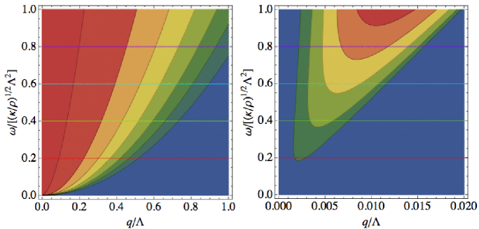
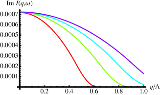
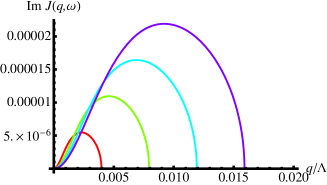
Figure 2: (Color online). Top: Plot of the imaginary part of the propagators $\tilde{I}(q,\omega)$ (left), and $\tilde{J}(q,\omega)$ (right) for $\lambda_{\rm e\text{-}fl}=0$ in the absence of the attractive part of the interaction. Bottom: Cuts of the same functions for for $\omega=0.2\omega_{\rm c},0.4\omega_{\rm c},0.6\omega_{\rm c}{\rm and}\,0.8\omega_{\rm c}$. Colors on the lower plots correspond to colors of the slices in the upper plots. Note that for $\tilde{J}(q,\omega)$, we have restricted the range of $q/\Lambda$ to small values.

We now discuss the flexural bubble $I_{0}(q,0)$ at finite temperature $T>0$, which allows to describe the quantum to classical crossover as a function of temperature. Evaluating $\tilde{K}_{0}(q,0)$ then allows to ascertain the importance of the anharmonic effects as a function of $T$ and wave vector $q$.

(i) classical, high $T$ limit: First we recall that in that limit the flexural bubble is UV convergent and given by (160),

$$I_{0}(q,0)=\frac{3}{16\pi}\frac{T}{\kappa^{2}q^{2}},$$ (63)

a well-known expression. It results in the classical RG equation

$$-q\partial_{q}\tilde{K}_{0}(q,0)=-\frac{3}{16\pi}\frac{T}{\kappa^{2}q^{2}}\tilde{K}_{0}^{2}(q,0),\quad{\rm classical},$$ (64)

which is exact in the $d=\infty$ limit. Comparing with (58) we see that in both cases the Young modulus is reduced at small $q$, but the classical, i.e. thermal, screening is much stronger than the quantum one. The classical anharmonic scale, defined from (60), is

$$q_{\rm anh}^{\rm clas}(T)^{2}=\frac{3}{16\pi}\frac{K_{0}T}{\kappa^{2}},$$ (65)

the well-known scale beyond which the standard SCSA predicts a softening of the elastic moduli of graphene.

(ii) arbitrary $T$: quantum to classical crossover: In Appendix B we obtain that

$$I_{0}(q,0)\simeq\frac{3\log\left(\frac{\Lambda}{2q}e^{3/4}\right)}{64\pi\kappa^{3/2}\sqrt{\rho}}+\frac{3}{16\pi}\frac{T}{\kappa^{2}q^{2}}\,g\!\left(\frac{\omega_{\rm fl}(q)}{8T}\right)$$ (66)

for $q\ll\Lambda$, and we recall the flexural phonon frequency $\omega_{\rm fl}(q)=q^{2}\sqrt{\kappa/\rho}$. The decreasing function $g(x)$, calculated in Appendix B, thus describes the thermal crossover from the classical result (63) with $g(0)=1,$ to the quantum one (53), with $g(\infty)=0$, as the temperature is decreased. The crossover scale extracted from the function $g(x)$ occurs for $q\approx q_{\rm Q}(T)$ with

$$q_{\rm Q}(T)^{2}={\color[rgb]{1.00,0.00,0.00}}T\sqrt{\frac{\rho}{\kappa}}.$$ (67)

i.e. , not surprisingly, the Debye scale. Smaller length scales show quantum behavior, while larger length scales behaves classically. Let us recall that the Debye temperature $T_{\Lambda}$ corresponds to $q_{\rm Q}(T_{\Lambda})=\Lambda,$ beyond which all scales behave classically. For $T$ of the order or larger than $T_{\Lambda}$ the crossover behaves differently (see Appendix B) however this is not relevant for graphene, where $T_{\Lambda}\approx 3400$K.

The structure of our result (66) is interesting: It can be interpreted as a sum of quantum and thermal fluctuations. When $T\gg\omega_{\rm fl}(q)$, i.e. $q<q_{\rm Q}(T)$ one obtains the direct sum of (53) and (63):

$$K_{0}I_{0}(q,0)\simeq\frac{3\lambda_{\rm anh}}{64\pi}\left[4\frac{q_{\rm Q}(T)^{2}}{q^{2}}+\ln\left(\frac{\Lambda}{q}\right)\right].$$ (68)

From now on we approximate $e^{3/4}/2\approx 1$. Note that at any finite $T$ the integral is UV divergent, hence (63) is recovered only when the thermal part overwhelms the quantum part, i.e. for $T>\frac{1}{4}\omega_{\rm fl}(q)\ln(\Lambda/q)$.

By contrast, at low $T$, the leading corrections are $O(T^{2})$ and using the results of Appendix B, we find

$$\!K_{0}I_{0}(q,0)\simeq\lambda_{\rm anh}\bigg{[}\frac{3}{64\pi}\log\left(\frac{\Lambda e^{3/2}}{q}\right)+\frac{3C}{2\pi}\frac{T^{2}}{\omega_{\rm fl}(q)^{2}}\bigg{]},$$ (69)

with $C=0.205617..$.

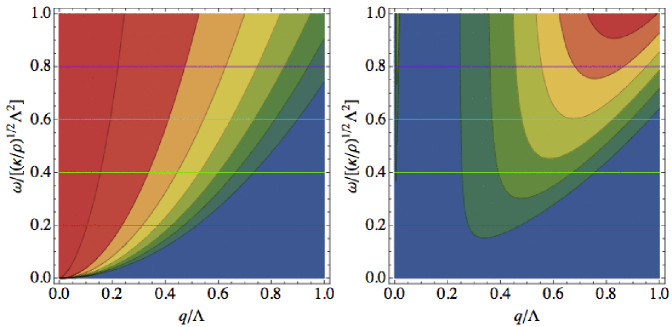
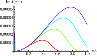
Figure 3: (Color online). Top: Plot of the imaginary part of the propagators $\tilde{I}(q,\omega)$ (left), and $\tilde{J}(q,\omega)$ (right) for $\lambda_{\rm e\text{-}fl}=10$ in the absence of the attractive part of the interaction. Bottom: Cuts of the same functions for for $\omega=0.2\omega_{\rm c},0.4\omega_{\rm c},0.6\omega_{\rm c}{\rm and}\,0.8\omega_{\rm c}$. Colors on the lower plots correspond to colors of the slices in the upper plots.

We now obtain the “phase diagram”, delimiting anharmonic/harmonic and quantum/classical regions in the $T,q$ plane. It is more conveniently expressed in terms of the frequency (i.e. energy) variable

$$\omega_{a}(T)\leftrightarrow q_{\rm anh}(T),\quad\omega_{a}=\omega_{\rm fl}(q_{\rm anh})=q^{2}_{\rm anh}\sqrt{\kappa/\rho}\ ,$$ (70)

which is the root of the equation

$$\frac{1}{8}\ln\frac{T_{\Lambda}}{\omega_{a}}+\frac{T}{\omega_{a}}g\left(\frac{\omega_{a}}{8T}\right)=\frac{16\pi}{3\lambda_{\rm anh}}.$$ (71)

The curve $\omega_{a}(T)$ is represented in Fig 1. There the vertical axis measures $\omega_{a}$ in Kelvin, equivalently wavector squared $q_{\rm anh}^{2}$, with the correspondence $q_{\rm anh}^{2}=\frac{\omega_{a}}{100K}\times 0.14$ Å^-2. Below this curve anharmonic effects are important. We have also plotted the diagonal line $\omega_{a}=T$, which corresponds to the crossover $q^{2}=q^{2}_{Q}(T)$ from quantum (to the left) to classical (to the right). Two important features are:

(i) the curve $\omega_{a}(T)$ crosses the diagonal $\omega_{a}=T$ only if $\lambda_{\rm anh}<\lambda^{*}=\frac{16\pi}{3g(1/8)}\approx 24$.

(ii) the curve $\omega_{a}(T)$ is asymptotic at high $T$ to a straight line with a slope $z$, solution of $\frac{1}{z}g(z/8)=\frac{16\pi}{3\lambda_{\rm anh}}$. Hence at high $T$, $\omega_{a}(T)\simeq zT$ with

$$z\simeq\frac{3\lambda_{\rm anh}}{16\pi}\approx\lambda_{\rm anh}/16.8\ ,\quad\lambda_{\rm anh}\ll\lambda^{*}$$ (72)

$$z\simeq\sqrt{\frac{24C\lambda_{\rm anh}}{16\pi}}\approx\sqrt{\lambda_{\rm anh}/10.5}\ ,\quad\lambda_{\rm anh}\gg\lambda^{*}~{}~{}~{}~{}~{}~{}$$ (73)

and $z=1$ for $\lambda=\lambda^{*}$.

Hence, as a function of $\lambda_{\rm anh}$, we can distinguish three regimes, represented in Fig 1:

(i) small $\lambda_{\rm anh}\ll\lambda^{*}$: The value of $q_{\rm anh}(T=0)$ is immeasurably small, hence $\omega_{a}(T)$ is essentially a straight line lying well below the diagonal. There are three regions QH, CH and CA (from left-up to right-down). Observing the region QA would require gigantic length scales.

(ii) moderate $\lambda_{\rm anh}<\lambda^{*}$: The two curves now cross, hence there are now four regimes, although the region QA remains quite limited.

(iii) $\lambda_{\rm anh}>\lambda^{*}$: $\omega_{a}(T)$ lies above the diagonal. There are three regimes QH, QA and CA.

In summary, we have given here, for completeness, a general discussion of the crossover as a function of the anharmonic coupling $\lambda_{\rm anh}$. In graphene, however, the situation seems to be (i), i.e. small coupling. Note however that there is still some uncertainties on the value of the bare Young modulus since experiments extract a renormalized one. Also, while the present scenario seems robust, the precise values, e.g. of $\lambda^{*}$ will be affected by the renormalisation of $\kappa$, not taken into account here.

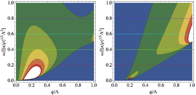
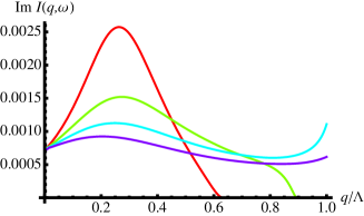
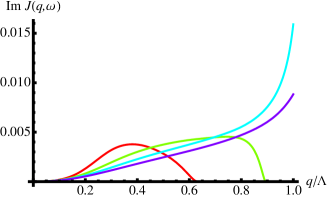
Figure 4: (Color online). Plot of the imaginary part of the propagators $\tilde{I}(q,\omega)$ (left), and $\tilde{J}(q,\omega)$ (right) for $\lambda_{\rm e\text{-}fl}=78$ in the absence of the attractive part of the interaction. Bottom: Cuts of the same functions for for $\omega=0.2\omega_{\rm c},0.4\omega_{\rm c},0.6\omega_{\rm c}{\rm and}\,0.8\omega_{\rm c}$. Colors on the lower plots correspond to colors of the slices in the upper plots.

IV.1.3 Finite frequency

In the quantum problem, the flexural bubble is interpreted as a two-phonon propagator, and it is interesting to work out its frequency dependence. Consider $T=0$. Performing the analytical continuation of the expressions in Appendix B to real time, we obtain in real frequency, the real part, as follows:

$${\rm Re}~{}I_{0}(q,\omega_{n}\to-i\omega+\delta) = \frac{1}{256\pi\kappa^{3/2}\sqrt{\rho}w}$$ (74)

$$\times\bigg{[}w\left(3\log\Big{|}(s-w+1)(s+w+1)\Big{|}-\left(w^{2}+12\right)\log\Big{|}w^{2}-4\Big{|}+\left(w^{2}+9\right)\log\Big{|}w^{2}-1\Big{|}+9\right)$$

$$~{}~{}~{}+4\log\bigg{|}\frac{s+w+1}{s-w+1}\bigg{|}+\left(6w^{2}+4\right)\log\bigg{|}\frac{w+1}{w-1}\bigg{|}-2\left(3w^{2}+4\right)\log\bigg{|}\frac{w+2}{w-2}\bigg{|}\bigg{]}.$$

We used the dimensionless variables

$$w:=\frac{2\sqrt{\rho}\omega}{\sqrt{\kappa}q^{2}}=\frac{2\omega}{\omega_{\rm fl}(q)},\qquad s:=\frac{4\Lambda^{2}}{q^{2}}.$$ (75)

The imaginary part reads

$${\rm Im}~{}I(p,i\omega_{n}\to\omega+i\delta)=\frac{\Theta(|w|<1+s)}{256\kappa^{3/2}\sqrt{\rho}w}\Big{[}(3|w|-4)\Theta(|w|-2)+(4-|w|)(|w|-1)^{2}\Theta(1<|w|<2)\Big{]}.$$ (76)

Hence it exhibits a two-threshold behavior. The lowest one ($w=1$) arises from the minimum energy $\omega=2\sqrt{\kappa/\rho}(\frac{q}{2})^{2}=\frac{1}{2}\omega_{\rm fl}(q)$ of a pair of flexural phonons with total momentum $q$, i.e. each with momentum $q/2$.

IV.2 Membrane coupled to electrons

We now study the coupled system.

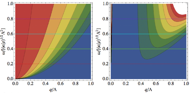
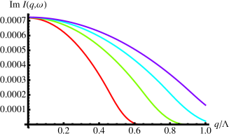
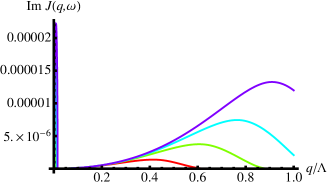
Figure 5: (Color online). Plot of the imaginary part of the propagators $\tilde{I}(q,\omega)$ (left), and $\tilde{J}(q,\omega)$ (right) for $\lambda_{\rm e\text{-}fl}=2.5$ in the presence of the attractive part of the interaction. Bottom: Cuts of the same functions for for $\omega=0.2\omega_{\rm c},0.4\omega_{\rm c},0.6\omega_{\rm c}{\rm and}\,0.8\omega_{\rm c}$. Colors on the lower plots correspond to colors of the slices in the upper plots.

IV.2.1 Qualitative discussion: pole in the two particle propagators

Schematically, the quartic interactions in our bare model are expressed in terms of the matrix ${\cal V}$,

$$\frac{1}{2d}\left(\begin{array}[]{cc}\frac{1}{2}{\rm P}^{\rm T}\partial h\partial h,&\delta\rho\end{array}\right)\left(\begin{array}[]{cc}K_{0}&-g\\ -g&V\end{array}\right)\left(\begin{array}[]{c}\frac{1}{2}{\rm P}^{\rm T}\partial h\partial h\\ \delta\rho\end{array}\right),$$ (77)

where $\delta\rho=\rho-\rho_{0}$ are the deviations from the uniform electron density. One legitimate question is whether the bare interaction matrix ${\cal V}$ is positive definite. In previous work Gazit (2009a); San-Jose et al. (2011) the electron degrees of freedom were integrated over within a Gaussian approximation before integrating over the in-plane phonon modes. It is easy to reproduce these manipulations in our framework. Integrating (77) over $\delta\rho$ assuming a Gaussian distribution schematically leads to

$$\frac{1}{2d}\left(K_{0}-\frac{g^{2}}{V}\right)\left(\frac{1}{2}{\rm P}^{\rm T}\partial h\partial h\right)^{2}.$$ (78)

i.e. a $q$-dependent Young modulus $K_{0}(q)=K_{0}-g^{2}/V(q)$. If one inserts $V(q)=\frac{2\pi e^{2}}{|q|}-\frac{g_{0}^{2}}{\lambda+2\mu}$ and $g=\frac{2\mu}{2\mu+\lambda}g_{0}$ one recovers the expression for the effective, $q$-dependent Young modulus $K_{0}(q)$ displayed in Gazit (2009a); San-Jose et al. (2011); it becomes negative for

$$\frac{\mu+\lambda}{2\mu+\lambda}q_{0}<q<q_{0}\quad,\quad q_{0}=\frac{2\pi e^{2}(2\mu+\lambda)}{g_{0}^{2}}$$ (79)

More generally, without integrating over the electrons, this signals negative modes for the interaction matrix ${\cal V}$, modes which are a mixture of the Gaussian curvature, and the electron density.

The fact that the bare quartic interaction matrix has negative modes does not necessary imply that the system is unstable, since one has to take into account thermal and quantum fluctuations. First, ${\cal V}$ is replaced by $\tilde{\cal V}$ which, in the large-$d$ limit, takes into account the bubbles (which contain the leading fluctuations). One has

$$\det\tilde{\cal V}=\frac{\det{\cal V}}{D},\qquad D=\det(1{\rm l}+{\cal J}{\cal V}),$$ (80)

where $D$ is the determinant defined in Eqs. (41)-(42). For the decoupled system, $D>0$. In this article, we claim that upon increasing the coupling, the true instability occurs not when $\det{\cal V}=0$, but at the critical mode $q_{\rm c}$ where

$$D(q_{\rm c},\omega=0)=0.$$ (81)

Since

$$\det\tilde{\cal J}=\frac{\det{\cal J}}{D}\ ,$$ (82)

this is equivalent to the appearance of a pole in the matrix (52) of the 2-particle propagators, i.e. of the 2-point functions for the composite fields $\frac{1}{2}{\rm P}^{\rm T}\partial h\partial h$ and $\delta\rho$. A coupled soft mode appears for these composite fields at zero frequency, signaling a phase transition. In section V we argue that the instability makes the composite fields acquire a non-zero expectation value in the ordered phase, at the wave vector $q_{\rm c}$, in analogy with a charge-density wave.

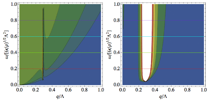
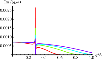
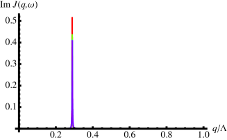
Figure 6: (Color online). Plot of the imaginary part of the propagators $\tilde{I}(q,\omega)$ (left), and $\tilde{J}(q,\omega)$ (right) for $\lambda_{\rm e\text{-}fl}=6$ in the presence of the attractive part of the interaction. Bottom: Cuts of the same functions for for $\omega=0.2\omega_{\rm c},0.4\omega_{\rm c},0.6\omega_{\rm c}{\rm and}\,0.8\omega_{\rm c}$. Colors on the lower plots correspond to colors of the slices in the upper plots.

IV.2.2 Results at finite frequency and collective excitations at $T=0$

Let us start by studying the dependence in (real) frequency and momentum of the dressed 2-particle propagators. In particular, we focus on their imaginary parts ${\rm Im}\tilde{I}(q,\omega)$ and ${\rm Im}\tilde{J}(q,\omega)$ which gives the weights of the collective 2 particle excitations in the phonon and electronic sectors, respectively. These propagators are defined by the equation

$$\left(\begin{array}[]{cc}\frac{1}{2}\tilde{I}(q,\omega)&\Pi(q,\omega)\\ \Pi(q,\omega)&N_{\rm f}\tilde{J}(q,\omega)\end{array}\right)=\left(\begin{array}[]{cc}\frac{1}{2}I_{0}(q,\omega)&0\\ 0&N_{\rm f}J_{0}(q,\omega)\end{array}\right)$$ (87)

$$~{}~{}~{}~{}\times\left[1{\rm l}{+}\left(\begin{array}[]{cc}K_{0}&{-}g\\ {-}g&V(q)\end{array}\right)\left(\begin{array}[]{cc}{\frac{1}{2}}I_{0}(q,\omega)&0\\ 0&{N_{\rm f}}J_{0}(q,\omega)\end{array}\right)\right]^{-1}$$ (92)

The real and imaginary parts of the flexural bubble $I_{0}$ at $T=0$ are given in (74) and (76). The bubble for the Dirac fermions has been calculated in several articles Gonzalez et al. (1994); Castro Neto et al. (2009) and its calculation is recalled in Appendix C. Upon continuation to real time it reads:

$${\rm Re}~{}J_{0}(q,\omega_{n}\to-i\omega+\delta)=\theta(v_{\rm F}q-|\omega|)\frac{q^{2}}{16\sqrt{v_{\rm F}^{2}q^{2}-\omega^{2}}}$$

(93)

$${\rm Im}~{}J_{0}(q,\omega_{n}\to-i\omega+\delta)=$$

$$\qquad~{}~{}~{}~{}~{}~{}~{}~{}{\rm sgn}(\omega)\theta(|\omega|-v_{\rm F}q)\frac{q^{2}}{16\sqrt{\omega^{2}-v_{\rm F}^{2}q^{2}}}.$$ (94)

We plot in figures 2-6 the imaginary parts of the dressed 2-particle propagators ${\rm Im}\tilde{I}(q,\omega)$ and ${\rm Im}\tilde{J}(q,\omega)$.

We first give the results when the electron-electron interaction is purely Coulomb, i.e. for $V(q)=V_{0}(q)$, disregarding the attraction induced by the in-plane phonons in Eq. (9). Results in the absence of the coupling $\lambda_{\rm e\text{-}fl}=0$, are plotted for reference in Fig. 2. This figure and the ones below display the imaginary part of the propagators, which can be interpreted as the density of excitations, which, in the case of flexural phonon pairs, is weighted by a matrix element, involving the transverse projector. These quantities could, in principle, be measured in inelastic scattering experiments. Note that the scale in $q/\Lambda$ of Fig. 2 is much expanded as compared to the following figures, since the peak characteristic of pure fermionic excitations takes place at a small momentum. The results at intermediate coupling, $\lambda_{\rm e\text{-}fl}=10,$ but still below the phase transition, are shown in Fig. 3. One sees the appearance of some structure in ${\rm Im}\tilde{J}$, at momenta well above the $\lambda_{\rm e\text{-}fl}=0$ peak of Fig. 2; the latter however survives (it is hard to see because of the different scales of $q/\Lambda$). Note that in the presence of a membrane-electron coupling, these plots show the total density of excitations projected either on the electronic degrees of freedom, or on the phonon degrees of freedom. One can imagine different experimental setups to measure either of them. Finally, the results for a coupling just above the phase transition, $\lambda_{\rm e\text{-}fl}=78$, (see below) are shown in Fig. 4. The results beyond the transition point should be interpreted with some care, since the calculation does not take into account the existence of a broken symmetry phase, discussed in the next sections. However, it is still informative since the high-energy excitations should remain unaffected by the low-energy changes induced by the phase transition.

Unless explicitly mentioned otherwise, the choice of parameters in plotting all the figures in this paper is the one in (14), with $\lambda_{\rm anh}=0.63$ and $\alpha_{e}=2,$ which corresponds to unscreened graphene. (Screening is examined below).

It appears clearly on these figures that the electron-hole pairs and the flexural phonons become more and more hybridized as the coupling increases, leading to collective excitations of mixed character.

We then give the results taking into account the attraction induced by the in-plane phonons in Eq. 9. As discussed previously, the attractive interaction does not depend on momentum, and it overcomes the repulsive Coulomb interactions for sufficiently large momenta. This affects significantly the instability, which also occurs at a finite momentum. The value of the critical coupling constant is considerably reduced, and the transition is much facilitated and occurs for realistic values of the parameters. The results for a coupling $\lambda_{\rm e\text{-}fl}=2.5$ near but below the phase transition are shown in Fig. 5. The results for a coupling $\lambda_{\rm e\text{-}fl}=6$ above the phase transition are shown in Fig. 6. Again, these low-energy spectra at large $\lambda_{\rm e\text{-}fl}$ beyond the transition cannot be taken at face value since they do not include effects from the phase transition. Note however that the spectral weight is concentrated on the region of momenta where the unstable modes appear.

IV.2.3 Results at zero frequency, phase transition for pure Coulomb interaction

When the coupling increases beyond a critical value, $D$ vanishes and a pole appears in the 2-particle excitations. The phase transition is defined by the appearance of a zero in

$$\!\!\!\!0 =\lim_{\omega\rightarrow 0}D(q,\omega)$$

$$=\lim_{\omega\rightarrow 0}{\rm\det}\!\left(\begin{array}[]{cc}1{+\frac{1}{2}}K_{0}I_{0}(q,\omega)&-g{N_{\rm f}J_{0}(q,\omega)}\\ -\rule{0.0pt}{10.76385pt}{\frac{1}{2}gI_{0}(q,\omega)}&1+V(q)N_{\rm f}J_{0}(q,\omega)\end{array}\right).$$ (97)

In this section we analyze this condition when the electron-electron interaction is purely Coulomb, i.e. for $V(q)=V_{0}(q)=\frac{2\pi e^{2}}{|q|}$, disregarding the attraction induced by the in-plane phonons in Eq. (9).

Let us start with $T=0$. Using the results (and definitions) (53)ff. for the phonon-bubble at zero frequency,

$$J_{0}(q,0)=\frac{|q|}{16v_{\rm F}},$$ (98)

and the dimensionless coupling constants of Eq. (12) we find

$$D(q,0) = \left(1+\frac{\pi N_{\rm f}}{8}\alpha_{\rm e}\right)\left[1+\lambda_{\rm anh}\frac{3}{128\pi}f(s)\right]$$ (99)

$$-\lambda_{\rm e\text{-}fl}^{2}\frac{N_{\rm f}}{16}\frac{3}{64\pi}\frac{1}{\sqrt{s}}f(s).$$

We recall that $s=4\Lambda^{2}/q^{2}$. Since in the present case $\lambda_{\rm anh}\frac{3}{64\pi}\approx 10^{-2}$ a reasonable approximation is to neglect the corresponding term. We note that $\frac{1}{\sqrt{s}}f(s)$ is maximal for $s_{\rm c}=18.5413$ and there equal to $0.205317$. Hence the wave-vector where the effect of the coupling is maximal is $q=q_{\rm c}^{\rm first}=2\Lambda/\sqrt{s_{\rm c}}=0.464472\Lambda$. This wave vector is not particularly small, but is well within the Brillouin zone. This implies that for

$$\lambda_{\rm e\text{-}fl}^{2}\geq 4.87052\frac{64\pi}{3}\left(\frac{16}{N_{\rm f}}+2\pi\alpha_{\rm e}\right),$$ (100)

modes around $q=q_{\rm c}$ become unstable, while $q_{\rm c}$ is the first unstable mode. Taking $N_{\rm f}=4$ and $\alpha_{\rm e}=2,$ we obtain the critical coupling as

$$\lambda_{\rm e\text{-}fl,c}\approx 73.5,$$ (101)

while for non-interacting electrons one would find by setting $\alpha_{e}=0$:

$$\lambda_{\rm e\text{-}fl,c}\approx 36.13.$$ (102)

Hence by screening the electron-electron interaction with a substrate renders the transition easier.

If one increases $\lambda_{\rm e\text{-}fl}$ beyond its critical value, a broader range of wave vectors becomes unstable. Larger wavelengths become available for the ripple instability. For instance, for $\lambda_{\rm e\text{-}fl}=80,$ the minimum instable vector is $q^{\rm min}_{\rm c}=0.217\Lambda$, while for $\lambda_{\rm e\text{-}fl}=100$, this value decreases to $q^{\rm min}_{\rm c}=0.09\Lambda$.

To confirm these results we plot in Fig. 7 the evolution of $D(q,0)$ for various couplings and various effective electron charges $\alpha_{e}$. The analysis of the eigenvectors of the matrix in (97), i.e. $1{\rm l}+{\cal J}{\cal V}$ (whose determinant is $D(q,0)$) at the wavevector $q_{c}$ where the transition occurs (with $D(q_{c},0)=0$) describes the nature of the collective excitation which becomes unstable. A simple numerical calculation using the above formulae, not detailed here, shows that this mode has a mixed electron-pair and flexural phonon pair character, with the amplitudes in either channel of the same order of magnitude.

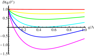
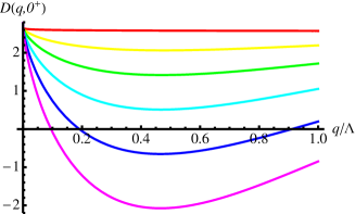
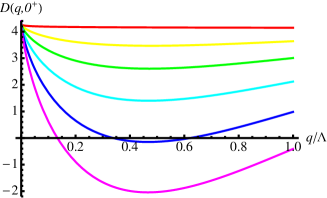
Figure 7: (Color online). Function $D(q,0)$ as defined in Eq. (97), in the absence of the attractive part of the interaction for various dimensionless coupling $\lambda_{\rm e\text{-}fl}$ increasing from top (red) to bottom (violet) Left: $\alpha_{e}=0.5$, for $\lambda_{\rm e\text{-}fl}=0,18,27,36,45,54$, Center: $\alpha_{e}=1$, for $\lambda_{\rm e\text{-}fl}=0,26,39,52,65,78$, Right: $\alpha_{e}=2$, for $\lambda_{\rm e\text{-}fl}=0,30,45,60,75,90$.

From the discussion in Section IV.1.2 we see that thermal effects cannot be neglected at wave-vectors of the order of $q_{\rm c}$. Hence the $T=0$ picture must be modified, whenever

$$T>T_{\Lambda}\frac{q_{\rm c}^{2}}{4\Lambda^{2}}\ln\!\left(\frac{2\Lambda}{q_{\rm c}}\right)\approx\frac{\ln 4}{16}T_{\Lambda}\approx 295\,{\rm K},$$ (103)

$$T_{\Lambda}=\sqrt{\frac{\kappa}{\rho}}\Lambda^{2}=0.31T_{1{\rm eV}}=3400\,{\rm K},$$ (104)

with $T_{1{\rm eV}}=11605\rm\,K$. However, thermal effects may modify it before that. To study the temperature dependence let us assume that $I_{0}(q,0)$ is given by its classical limit, with $\frac{1}{2}K_{0}I_{0}(q,0)=q_{a}^{2}/q^{2}$ and $q_{a}^{2}=\frac{3}{32\pi}\frac{K_{0}T}{\kappa^{2}}$. Then

$$D(q,0)=\left(1+\frac{\pi N_{\rm f}}{8}\alpha_{\rm e}\right)\left(1+\frac{q_{a}^{2}}{q^{2}}\right)-\lambda_{\rm cl}^{2}\frac{N_{\rm f}}{16}\frac{q_{a}^{2}}{\Lambda q}$$ (105)

in terms of the classical dimensionless coupling $\lambda_{\rm cl}=\lambda_{\rm e\text{-}fl}/\sqrt{\lambda_{\rm anh}}$. The transition occurs when

$$\lambda_{\rm cl}^{2}>\frac{4\Lambda}{q_{a}}\left(\frac{8}{N_{\rm f}}+\pi\alpha_{\rm e}\right)$$ (106)

for the wave-vector $q_{\rm c}=q_{a}$. This gives

$$\lambda_{\rm cl,c}=\frac{6.54}{T[\rm eV]},$$ (107)

which is consistent with the above estimates. One should check whether the fermion bubble remains the same until these temperatures, see Appendix C.

IV.2.4 Results at zero frequency, phase transition in presence of an attraction

As we now discuss, the attractive interaction between electrons generated by the integration over the in-plane phonons, i.e.

$$\frac{2\pi e^{2}}{q}\to\frac{2\pi e^{2}}{q}-\frac{2\mu+\lambda}{4\mu^{2}}g^{2},$$ (108)

dramatically lowers the value of the coupling necessary to induce the phase transition. Equation (108) can be rewritten as

$$\frac{2\pi e^{2}}{q}\to\frac{2\pi e^{2}}{q}\left[1-\frac{q}{2\pi\Lambda\alpha_{\rm e}}\left(1+\frac{\lambda}{\mu}\right)\lambda_{\rm cl}^{2}\right].$$ (109)

With these replacements, equation (105) becomes

$$D(q,0) = \left[1+\frac{\pi N_{\rm f}}{8}\alpha_{\rm e}-\frac{N_{\rm f}}{8}\frac{1}{\sqrt{s}}\left(1+\frac{\lambda}{\mu}\right)\lambda_{\rm cl}^{2}\right]$$ (110)

$$\times\left[1+\lambda_{\rm anh}\frac{3}{128\pi}f(s)\right]$$

$$-\lambda_{\rm e\text{-}fl}^{2}\frac{N_{\rm f}}{16}\frac{3}{64\pi}\frac{1}{\sqrt{s}}f(s).$$

If we again neglect the anharmonic corrections, we obtain

$$D(q,0)\approx 1 + \frac{\pi N_{\rm f}}{8}\alpha_{\rm e}$$ (111)

$$- \frac{N_{\rm f}}{8\sqrt{s}}\left[\Big{(}1+\frac{\lambda}{\mu}\Big{)}\lambda_{\rm cl}^{2}+\lambda_{\rm e\text{-}fl}^{2}\frac{3}{128\pi}f(s)\right]\!.~{}~{}~{}~{}~{}~{}~{}$$

Further neglecting the last term, we find that the first instability occurs near the cutoff $s_{\rm c}=4$ when $\lambda_{\rm cl}$ reaches the critical value

$$\lambda_{\rm cl,c}^{2}=\frac{2}{1+\frac{\lambda}{\mu}}\left(\frac{8}{N_{\rm f}}+\pi\alpha_{\rm e}\right),$$ (112)

hence using $N_{f}=4$ and $\alpha_{e}=2$ at

$$\lambda_{\rm cl,c}\approx 3.8\ .$$ (113)

On the other hand, if we use $\lambda_{\rm anh}=0.63$, we find

$$\lambda_{\rm e-fl}\approx 3\ .$$ (114)

As announced, this is a much lower critical value than the typical critical coupling values found above. The first instability however occurs this time for $q_{\rm c}=\Lambda$. This can be seen in Fig. 8 where we have plotted how $D(q,0)$ evolves with the coupling constant for various values of the effective electron charge $\alpha_{\rm e}$. Again, larger values $\lambda_{\rm cl}>\lambda_{\rm cl,c}$ result in smaller wave vectors becoming unstable. Thus, although the criterion for the transition $D(q_{c},0)=0$ is different from the one used in previous articles, we do find that this transition is facilitated by the electronic attraction mediated by the in-plane phonons, an effect which has a counterpart as $K_{0}(q)$ becoming negative at some wave-vector, as discussed in Section IV.2.1.

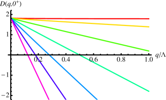
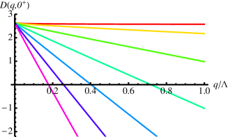
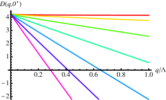
Figure 8: (Color online). Function $D(q,0)$ as defined in Eq. (97), in presence of the attractive part of the interaction for dimensionless coupling $\lambda_{\rm e\text{-}fl}=0,1,2,3,4,5,6$, from top (red) to bottom (violet). Left: $\alpha_{e}=0.5$. Center: $\alpha_{e}=1$. Right: $\alpha_{e}=2$.

V saddle point: beyond the instability

V.1 The saddle-point equations

In this section we study the free energy of the model at $d=\infty$. As is well known from the $O(N)$ model at large $N$ the saddle-point equations allow to determine whether a non-trivial minimum exists, signaling a non-trivial phase with ripples.

To this aim we introduce fluctuating auxiliary fields $\sigma(x,\tau)$ and $\alpha(x,\tau)$ and consider the (e.g.  Matsubara) action

$$S^{\prime} = S_{0}+S^{\prime}_{\rm int}$$ (115)

$$S^{\prime}_{\rm int} = \int_{x\tau}\sigma\left[\frac{1}{2}{\rm P}^{\rm T}_{ij}(\partial)\sum_{a=1}^{d}\partial_{i}h_{a}\partial_{j}h_{a}\right]+\alpha\sum_{\gamma=1}^{dN_{\rm f}}\bar{\Psi}_{\gamma}1{\rm l}\Psi_{\gamma}$$ (121)

$$\!\!\!\!\!\!-\frac{d}{2}\int_{xx^{\prime}\tau}\left(\begin{array}[]{cc}\sigma,&\alpha\end{array}\right)_{x\tau}\left(\begin{array}[]{cc}K_{0}&-g\\ -g&V\end{array}\right)^{-1}_{xx^{\prime}}\left(\begin{array}[]{c}\sigma\\ \alpha\end{array}\right)_{x^{\prime}\tau}.$$

The interaction matrix can be non-local but is assumed to be static (i.e. frequency independent). After integration over auxiliary fields it reproduces the action (III.1). As we show below, at the transition the fields $\sigma$ and $\alpha$ acquire static and space-dependent expectation values, which we denote $\sigma_{0}(x):=\langle\sigma(x,\tau)\rangle$ and $\alpha_{0}(x):=\langle\alpha(x,\tau)\rangle$. Since the theory is Gaussian in the auxiliary fields, we have the exact relations

$$\left(\begin{array}[]{c}\sigma_{0}(x)\\ \alpha_{0}(x)\end{array}\right)=\int_{x^{\prime}}\left(\begin{array}[]{cc}K_{0}&-g\\ -g&V\end{array}\right)_{xx^{\prime}}\left(\begin{array}[]{c}\Phi_{0}(x^{\prime})\\ \delta\rho_{0}(x^{\prime})\end{array}\right).$$ (122)

We have defined the expectation values

$$\frac{1}{d}\left<\sum_{a=1}^{d}{\rm P}^{\rm T}_{ij}(\partial)\partial_{i}h^{a}(x,\tau)\partial_{j}h^{a}(x,\tau)\right>=\Phi_{0}(x)\qquad$$ (123)

$$\frac{1}{d}\left<\sum_{\gamma=1}^{dN_{\rm f}}\bar{\Psi}_{\gamma}(x,\tau)1{\rm l}\Psi_{\gamma}(x,\tau)\right>-\rho_{0}=\delta\rho_{0}(x),$$ (124)

Hence the phase transition is equivalently characterized by these composite fields, the Gaussian curvature and the electronic charge density, acquiring expectation values, which are static and non-uniform in space. Since these order parameters are defined only at a non-zero wave-vector, they obviously vanish for the free action $S_{0}$. They also vanish in the small-$g$ phase. We show below that the pole in the coupled propagator of the composite fields ${\rm P}^{\rm T}\partial h\partial h$ and $\bar{\Psi}\Psi$ corresponds to an instability, allowing $\sigma_{0}(x)$ and $\alpha_{0}(x)$ to become non-zero.

We now derive the effective action for the fields $\sigma$ and $\alpha$. We allow for a breaking of the $O(d)$ symmetry, i.e. the vector field $h_{a}(x,\tau)$ may acquire a non-zero expectation value and pick one direction in the transverse space, denoted $a=1$, with $\langle h_{a}(x,\tau)\rangle=\delta_{a1}h_{1}(x,\tau)\neq 0$. For the physical model $d=1$ this is the Ising symmetry related to the two possible orientations of the normal vector. There are various equivalent ways to implement that breaking, either by integrating over the $d-1$ flexural modes except $h_{1}$, see Zinn-Justin (1989), section 26, or decomposing $h_{a}(x,\tau)=\langle h_{a}(x,\tau)\rangle+\delta h_{a}(x,\tau)$ into an average and a fluctuating part.

Integrating over the fermions and the fluctuating part of the flexural modes, we find that the action reads, in the large-$d$ limit,

$$\frac{S^{\prime}}{d}=\frac{1}{2}\mathrm{tr}\ln\left(-\rho\partial_{\tau}^{2}+\kappa\nabla^{4}-[{\rm P}^{\rm T}_{ij}(\partial)\sigma(x,\tau)]\partial_{i}\partial_{j}\right)$$

$$-\frac{N_{\rm f}}{2}\mathrm{tr}\ln\Big{(}-v_{\rm F}[{\boldsymbol{\sigma}}\cdot(-i\nabla)]+\left[\alpha(x,\tau)-\mu-\partial_{\tau}\right]1{\rm l}\Big{)}$$

$$-\frac{1}{2}\int_{x,x^{\prime},\tau}\left(\begin{array}[]{cc}\sigma,&\alpha\end{array}\right)_{x\tau}\left(\begin{array}[]{cc}K_{0}&-g\\ -g&V\end{array}\right)_{xx^{\prime}}^{-1}\left(\begin{array}[]{c}\sigma\\ \alpha\end{array}\right)_{x^{\prime}\tau}$$ (130)

$$+\frac{1}{d}\int_{x,\tau}\left[\frac{\kappa}{2}(\nabla^{2}h_{1})^{2}+\frac{\rho}{2}(\partial_{\tau}h_{1})^{2}+\sigma\frac{1}{2}{\rm P}^{\rm T}_{ij}(\partial)\partial_{i}h_{1}\partial_{j}h_{1}\right].$$

(131)

We have used that there are several ways to rewrite the term containing the transversal projector,

$$\int_{x\tau}\sigma(x,\tau){\rm P}^{\rm T}_{ij}(\partial)\left[\partial_{i}h(x,\tau)\partial_{j}h(x,\tau)\right]$$

$$=\int_{x\tau}\left[{\rm P}^{\rm T}_{ij}(\partial)\sigma(x,\tau)\right]\partial_{i}h(x,\tau)\partial_{j}h(x,\tau)$$

$$=\int_{p,k,\omega,\omega^{\prime}}\sigma(p,\omega^{\prime}){\rm P}^{\rm T}_{ij}(p)k_{i}k_{j}h(-k,-\omega)h(k-p,\omega-\omega^{\prime})$$

$$=-\int_{x\tau}\left[{\rm P}^{\rm T}_{ij}(\partial)\sigma(x,\tau)\right]h(x,\tau)\partial_{i}\partial_{j}h(x,\tau)$$ (132)

If we suppose that $h_{1}\sim\sqrt{d}$, which is the usual scaling for $O(d)$ breaking, the action is uniformly proportional to $d$ and one can thus look for a saddle point.

We now derive the saddle-point equations. Since we look for a static solution, our ansatz is in terms of time-independent fields. The variation w.r.t. $\sigma(x,\tau)$ yields

$$\frac{1}{d}{\rm P}^{\rm T}_{ij}\partial_{i}h_{1}(x)\partial_{j}h_{1}(x)-\frac{1}{2\beta}\sum_{\omega_{n}}\mathrm{P}^{\rm T}_{ij}(\partial_{x})\partial_{xi}\partial_{xj}\bigg{[}\rho\omega_{n}^{2}+\kappa\nabla_{y}^{4}-[{\rm P}^{\rm T}_{ij}(\partial_{y})\sigma(y)]\partial_{iy}\partial_{jy}\bigg{]}^{-1}_{xx}=\int_{x^{\prime}}\Big{(}1,0\Big{)}\left(\begin{array}[]{cc}K_{0}&-g\\ -g&V\end{array}\right)_{\!xx^{\prime}}^{\!-1}\left({\sigma(x^{\prime})\atop\alpha(x^{\prime})}\right).$$ (133)

The variation w.r.t. $\alpha$ yields, setting the chemical potential $\mu\to 0$,

$$N_{\rm f}\frac{1}{\beta}\sum_{\omega^{\prime}_{n}}(i\omega^{\prime}_{n})[(-\alpha(y)+i\omega^{\prime}_{n})^{2}+\nabla_{y}^{2}]^{-1}_{xx}$$

$$=\int_{x^{\prime}}\Big{(}0,1\Big{)}\left(\begin{array}[]{cc}K_{0}&-g\\ -g&V\end{array}\right)_{xx^{\prime}}^{-1}\left({\sigma(x^{\prime})\atop\alpha(x^{\prime})}\right).$$ (136)

Finally, the variation w.r.t. $h_{1}$ yields

$$\kappa k^{4}h_{1}(k)+\int_{p}\left(k^{2}-\frac{(k\cdot p)^{2}}{p^{2}}\right)\sigma({p)}h_{1}(k-p)=0\ .$$ (137)

Clearly there is always the trivial solution to these equations $\sigma(x)=\alpha(x)=h_{1}(x)=0,$ which corresponds to the weak-coupling phase. Consider now the action $\frac{1}{d}S^{\prime}[\sigma,\alpha,h_{1}]$ in this phase, as a functional of the fields. It is easy to see by expanding Eq. (131) in powers of $\sigma$ and $\alpha$ that

$$\frac{S^{\prime}[\sigma,\alpha,h_{1}=0]}{d} = -\frac{d}{2}\left(\begin{array}[]{cc}\sigma,&\alpha\end{array}\right)({\cal J}+{\cal V}^{-1})\left(\begin{array}[]{c}\sigma\\ \alpha\end{array}\right)$$ (142)

$$+{\cal O}((\sigma,\alpha)^{3}),$$

where ${\cal J}$ is the matrix of bubbles introduced in Eq. (36). Now from the relations given there, one finds that, in terms of the dressed interaction,

$${\cal J}+{\cal V}^{-1}={\cal V}^{-1}(1{\rm l}+{\cal V}{\cal J})=\tilde{\cal V}^{-1}.$$ (143)

The important point is that if $D=\det(1{\rm l}+{\cal V}{\cal J})$ vanishes at $q=q_{c}$, then the quadratic part of the action in $(\sigma,\alpha)$ has a zero mode at $q=q_{c}$, and the solution $\sigma(x)=\alpha(x)=0$ becomes unstable. The same instability can also be seen on the above saddle-point equations expanded to linear order in $(\sigma,\alpha)$. Hence the vanishing of the determinant, demonstrated in Section IV.2 implies a phase transition, and that one must look for a non-trivial solution of the saddle-point equations.

Note, from (142), that we did not need to allow for a non-vanishing $h_{1}$ to find the instability. Indeed, to quadratic order the $(\sigma,\alpha)$ and $h_{1}$ sectors decouple, since the leading coupling is $O(\sigma h_{1}^{2})$. Whether $h_{1}$ acquires or not an expectation value beyond the instability – i.e. whether the rippling and breaking of Ising symmetry (here $O(d)$ symmetry) occur simultaneously or not – remains to be investigated.

Searching for a solution of the above saddle-point equations in the rippled phase is beyond the goal of this article. In Appendix D however, we remark that the magnitude of $\sigma$ fixes a scale for a possible $O(d)$ symmetry breaking.

VI Conclusion

In conclusion, we have studied in this article a model for graphene as an elastic membrane coupled to Dirac electrons. By extending the model to $d$-component flexural phonons and $N_{\rm f}d$-component Dirac fermions, we obtained a solvable limit for large $d$, while retaining a lot of the physics, e.g. screening of non-linearities by thermal and quantum fluctuations. We derived the Self Consistent Screening Approximation (SCSA) equations, which are extensions of the standard classical SCSA equations to (i) the quantum membrane, and (ii) the coupled quantum membrane-electron problem.

By a careful study of the temperature dependence of the flexural bubble we obtained the first controlled description of the quantum to classical, and harmonic to anharmonic crossover for the problem of the membrane alone.

We have analyzed, within the same approximation, the effect on the membrane of the electronic degrees of freedom. We find that the electron excitations, i.e. the electron-hole pairs, mix with the flexural modes, leading to collective excitations of hybrid character. For sufficiently large values of the electron-phonon coupling, new modes appear below the continuum of excitations made up of two flexural phonons. As the coupling is increased, the frequency of these modes goes to zero at a finite value of the momentum $q_{c}$. If the coupling is increased further, the frequency of the modes within a range of finite momenta becomes imaginary, signalling a phase transition and the appearance of a broken symmetry phase.

The instability appears first at momenta comparable with the high-momentum cutoff, of the order of the lattice spacing. As the electron-phonon coupling increases, the range of unstable modes shifts towards lower momenta. The character of these modes changes between mostly phonon-like to electron-like.

We have found that the attractive interaction between electrons mediated by in-plane phonons greatly facilitates the transition which then occurs at lower and quite realistic values of the coupling. In addition, the transition is also found to be facilitated by screening of the Coulomb interaction.

Evidence for this instability was demonstrated in the $d=\infty$ limit. It is different from previous approaches, because it does not involve the renormalization of the bending rigidity San-Jose et al. (2011) and it does not rely on the effective Young modulus becoming negative in some window of wave vectors Gazit (2009a).

It is tempting to associate this transition to the spontaneous and simultaneous formation of ripples coupled to electronic puddles. To make this more precise we have derived the saddle-point equations, exact at $d=\infty$, which allow us to study the transition and in principle to describe the rippled phase. It confirms that the instablility occurs at a finite wave-vector and mixes electronic and flexural degrees of freedom. The study of the coupled non-linear saddle-point equations which describe the rippled phase is however complicated, and left for the future. (It could be done either numerically or in some expansion, e.g. for large coupling.). We have not studied here the renormalization of $\kappa,\rho,g,v_{\rm F}$, which can be added and occurs to next order in $1/d$. Although we do not expect renormalization to qualitatively change the mechanism proposed here, it is likely to change the estimates for the transition.

The results presented here confirm that the coupling between flexural modes and electron-hole pairs significantly changes the structural properties of graphene. The main changes, and the instability for sufficiently large couplings, occur at a finite momentum. Hence, the results reported here should not be modified by the presence of a finite carrier concentration, provided that the square root of the density of carriers is small compared to the wave vector at which the instability takes place. On the other hand, the existence of a gap comparable to the bandwidth or the electronic cutoff will suppress the effects reported here. The two-dimensional material boron nitride is structurally very similar to graphene, but it has a larger gap in the electronic spectrum. It would be interesting to analyze the properties of free standing boron nitride. Other two dimensional systems, like MoS₂ or MoW₂ are semiconductors with a small gap. Their tendency towards ripple formation should be intermediate between that of graphene and of boron nitride.

An interesting extension would be to apply our approach in the presence of a substrate. Indeed it is known that graphene on many metallic substrates, where the Coulomb interaction is screened, has long-ranged height corrugations de Parga et al. (2008). The study of these corrugations requires to add to our model the interaction between graphene and the substrate.

Appendix A Integration over in-plane phonons

We start from the elastic energy (1) plus the coupling term (4), together with their associated Matsubara actions. For notational simplicity we will omit the index $a=1,...,d$, and set $\partial h_{a}\partial h_{a}\to\partial h\partial h$, i.e. in practice we consider only the physical case $d=1$, while the index can easily be restored at the end. We note that the total coupling of the in-plane displacements to the flexural modes and electron density can be written, upon integration by part, as

$$S_{\rm u\text{-}fl,e}=\int\mathrm{d}^{2}x\,\mathrm{d}\tau\,~{}u_{m}[-A_{ijm}(\partial)\partial_{i}h\partial_{j}h+g\partial_{m}\delta\rho].$$ (144)

Hence integrating over in-plane modes $u_{i}$ we find the total effective Matsubara action for the flexural modes,

$$S_{\rm eff,fl}=\frac{1}{8}\int\mathrm{d}^{2}x\,\mathrm{d}\tau\,[\lambda(\partial_{i}h\partial_{i}h)^{2}+2\mu(\partial_{i}h\partial_{j}h)^{2}]-\frac{1}{2}\int_{q,\omega}(\partial_{i}h\partial_{j}h)_{q,\omega}(\partial_{k}h\partial_{l}h)_{-q,-\omega}A_{ijm}(q)A_{klp}(q)\langle u_{m}(q,\omega)u_{p}(-q,\omega)\rangle_{0}.$$ (145)

Here and above we denote $A_{ijm}(q)=\frac{\lambda}{2}\delta_{ij}q_{m}+\frac{\mu}{2}(q_{i}\delta_{jm}+q_{j}\delta_{im})$ and we use the notation $\int_{\omega}\equiv\frac{1}{\beta}\sum_{\omega_{n}}$. Inserting the quadratic bare in-plane phonon propagator gives

$$\langle u_{m}(q)u_{p}(-q)\rangle_{0}=\frac{P_{mp}^{L}(q)}{\rho\omega^{2}+(\lambda+2\mu)q^{2}}+\frac{P_{mp}^{T}(q)}{\rho\omega^{2}+\mu q^{2}}.$$ (146)

We find, after a tedious calculation,

$$S_{\rm eff,fl} = \int_{q,\omega}\frac{(\lambda+\mu)\mu q^{2}}{2(\rho\omega^{2}+\mu q^{2})(\rho\omega^{2}+(\lambda+2\mu)q^{2})}\Big{[}\mu q^{2}\Big{|}({\rm P}^{\rm T}\partial h\partial h)_{q,\omega}\Big{|}^{2}+\rho\omega^{2}({\rm P}^{\rm T}\partial h\partial h)_{q,\omega}(\partial h\partial h)_{-q,-\omega}\Big{]}$$

$$+\frac{(\lambda+2\mu)\rho\omega^{2}}{8(\rho\omega^{2}+(\lambda+2\mu)q^{2})}\Big{|}(\partial h\partial h)_{q,\omega}\Big{|}^{2}+\frac{\mu\rho\omega^{2}}{2(\rho\omega^{2}+\mu q^{2})}\Big{[}(\partial_{1}h\partial_{2}h)_{q,\omega}(\partial_{1}h\partial_{2}h)_{-q,-\omega}-(\partial_{1}h\partial_{1}h)_{q,\omega}(\partial_{2}h\partial_{2}h)_{-q,-\omega}\Big{]}.$$

We have used the notations $({\rm P}^{\rm T}\partial h\partial h)(x,\tau)={\rm P}^{\rm T}_{ij}(\partial)\partial_{i}h(x,\tau)\partial_{j}h(x,\tau)$ and $(\partial h\partial h)(x,\tau)=\partial_{i}h(x,\tau)\partial_{i}h(x,\tau)$ for the bilinears in the gradient of the height field, and their Fourier transforms. We have used that $\int_{q,\omega}(\partial_{1}h\partial_{2}h)_{q,\omega}(\partial_{1}h\partial_{2}h)_{-q,-\omega}=\int_{q,\omega}(\partial_{1}h\partial_{1}h)_{q,\omega}(\partial_{2}h\partial_{2}h)_{-q,-\omega}$ to rewrite some terms. An equivalent more compact form is given by

$$S_{\rm eff,fl} = \int_{q,\omega}\frac{4\mu(\lambda+\mu)q^{2}+\rho\omega^{2}(\lambda+2\mu)}{8((\lambda+2\mu)q^{2}+\rho\omega^{2})}|H^{T}(q,\omega)|^{2}$$ (148)

$$+\frac{1}{2}\rho\omega^{2}\bigg{[}\frac{(\lambda+2\mu)|H^{L}(q,\omega)|^{2}+2\lambda H^{L}(q,\omega)H^{T}(-q,-\omega)}{4((\lambda+2\mu)q^{2}+\rho\omega^{2})}+\frac{\mu|H^{M}(q,\omega)|^{2}}{\mu q^{2}+\rho\omega^{2}}\bigg{]},$$

where we have used the general decomposition of the matrix $H_{ij}=\partial_{i}h\partial_{j}h$,

$$H_{ij}(q,\omega)={\rm P}^{\rm T}_{ij}(q)H^{T}(q,\omega)+{\rm P}^{\rm L}_{ij}(q)H^{L}(q,\omega)+{\rm P}^{\rm M}_{ij}(q)H^{L}(q,\omega).$$ (149)

Here ${\rm P}^{\rm M}_{ij}(q):=(q_{i}q^{T}_{j}+q^{T}_{i}q_{j})/q^{2}$, with $q^{T}_{i}=\epsilon_{ij}q_{j}$, is not a projector but satisfies $({\rm P}^{\rm M})^{2}=1$ and is orthogonal to $\rm P^{T}$ and $\rm P^{L}$. We further define

$$H^{T}(x,\tau)={\rm P}^{\rm T}_{ij}(\partial)\partial_{i}h(x,\tau)\partial_{j}h(x,\tau),$$ (150)

$$H^{L}(x,\tau)={\rm P}^{\rm L}_{ij}(\partial)\partial_{i}h(x,\tau)\partial_{j}h(x,\tau),$$ (151)

$$H^{M}(x,\tau)=\frac{1}{2}{\rm P}^{\rm M}_{ij}(\partial)\partial_{i}h(x,\tau)\partial_{j}h(x,\tau).$$ (152)

We note that (A) and (148) lead to the usual result for $\omega=0$, i.e. in the classical (high $T$) limit, $S_{\rm eff,fl}=\frac{K_{0}}{8}|({\rm P}^{\rm T}\partial h\partial h)_{q,\omega}|^{2}$, with $K_{0}=4\mu(\lambda+\mu)/(\lambda+2\mu)$. The novelty is the appearance of a coupling to the longitudinal part of the tensor $\partial_{i}h\partial_{j}h$ which arises from an incomplete screening due to retardation effects. (This coupling is proportional to $\omega^{2}$).

Integration over in-plane modes also generates a cross-term

$$\delta S_{\rm eff,fl\text{-}e}=\int_{q,\omega}\frac{g}{(\lambda+2\mu)q^{2}+\rho\omega^{2}}q_{m}A_{ijm}(q)(\partial_{i}h\partial_{j}h)_{q,\omega}\delta\rho(-q,-\omega).$$ (153)

It has to be added to the direct coupling (4),

$$S_{\rm fl,e,direct}=-g_{0}\int\mathrm{d}^{2}x\,\mathrm{d}\tau\,\frac{1}{2}(\partial_{i}h\partial_{i}h)\delta\rho\ ,$$ (154)

and produces in total

$$S_{\rm fl,e} = -g_{0}\int_{q,\omega}\frac{2\mu q^{2}(\delta_{ij}-\hat{q}_{i}\hat{q}_{j})+\rho\omega^{2}\delta_{ij}}{(\lambda+2\mu)q^{2}+\rho\omega^{2}}$$ (155)

$$~{}~{}~{}~{}~{}~{}~{}~{}~{}\times\frac{1}{2}(\partial_{i}h\partial_{j}h)_{q,\omega}\delta\rho(-q,-\omega).~{}~{}~{}~{}~{}~{}$$

In the limit where one neglects the $\omega$ dependence (e.g. in the classical limit, as described in the text) it reduces to

$$S_{\rm fl,e}=-g_{0}\frac{2\mu}{\lambda+2\mu}\int\mathrm{d}^{2}x\,\mathrm{d}\tau\,\frac{1}{2}({\rm P}^{\rm T}_{ij}(\partial)\partial_{i}h\partial_{j}h)\delta\rho.$$ (156)

In addition integrating over the in-plane phonons generates a short-ranged attraction between electrons,

$$\delta S=-\frac{1}{2}g^{2}\int_{q,\omega}|\rho_{\rm el}(q,\omega)|^{2}\frac{q^{2}}{(\lambda+2\mu)q^{2}+\rho\omega^{2}}.$$ (157)

In the classical limit, or neglecting the frequency dependence, this gives the result (9) quoted in the text.

Finally, for completeness we should mention that there is also a fluctuation determinant, which gives an additional contribution to the Matsubara action,

$$\frac{1}{2}\mathrm{tr}\ln\!\Big{(}\rho\omega^{2}+(\lambda+2\mu)q^{2}\Big{)}+\frac{1}{2}\mathrm{tr}\ln(\rho\omega^{2}+\mu q^{2}),$$ (158)

a field-independent temperature dependent constant (which contributes to the specific heat) but which does not play an important role in our discussion in the text.

Appendix B Flexural bubble

Consider the flexural bubble

$$I_{0}(p,\omega)=\int_{k}\frac{1}{\beta}\sum_{\omega_{n}}\frac{\left[k^{2}-\frac{(k\cdot p)^{2}}{p^{2}}\right]^{2}}{[\kappa(k+\frac{p}{2})^{4}+\rho(\omega_{n}+\omega)^{2}][{\kappa(k-\frac{p}{2})^{4}+\rho(\omega_{n})^{2}}]},$$ (159)

where the summation is over the Matsubara frequencies $\omega_{n}=2\pi n/\beta$, $n\in\mathbb{Z}$.

First, in the high-temperature limit, zero Matsubara frequencies dominate, and (159) reduces to the classical result

$$I_{0}(p,\omega_{m})=\delta_{m,0}I_{0}(p)\quad,\quad I_{0}(p)=\frac{T}{\kappa^{2}}\int_{k}\frac{\left[k^{2}-\frac{(k\cdot p)^{2}}{p^{2}}\right]^{2}}{(k+\frac{p}{2})^{4}(k-\frac{p}{2})^{4}}=\frac{3}{16\pi}\frac{T}{\kappa^{2}p^{2}}\,,$$ (160)

which is a convergent integral. At finite temperature, where quantum effects are important, one must perform the summation over the Matsubara frequencies $\omega_{n}=2\pi n/\beta$. Using that $\omega=2\pi j/\beta$, with $j\in\mathbb{Z}$, and the symmetry $k\to-k$, one obtains

$$I_{0}(p,\omega)=-\int_{k}\left[k^{2}-\frac{(k\cdot p)^{2}}{p^{2}}\right]^{2}\frac{16\left[\kappa(k\cdot p)\left(4k^{2}+p^{2}\right)-\rho\omega^{2}\right]\coth\left(\frac{\beta\sqrt{\kappa}(2k+p)^{2}}{8\sqrt{\rho}}\right)}{\sqrt{\kappa}\sqrt{\rho}(2k+p)^{2}\left[4\kappa(k\cdot p)^{2}+\rho\omega^{2}\right]\left[\kappa\left(4k^{2}+p^{2}\right)^{2}+4\rho\omega^{2}\right]}.$$ (161)

It simplifies, for $\omega=0,$ into

$$I_{0}(p,\omega=0) = -\frac{1}{(2\pi)^{2}\kappa^{3/2}\sqrt{\rho}}\int_{0}^{\Lambda}\mathrm{d}k\int_{0}^{2\pi}\mathrm{d}\theta\frac{4k^{4}\sin^{3}(\theta)\tan(\theta)\coth\left(\frac{\beta\sqrt{\kappa}\left(4k^{2}+4kp\cos(\theta)+p^{2}\right)}{8\sqrt{\rho}}\right)}{p\left(4k^{2}+p^{2}\right)\left(4k^{2}+4kp\cos(\theta)+p^{2}\right)}$$ (162)

$$= -\int_{0}^{\Lambda/p}\mathrm{d}k\int_{-1}^{1}\mathrm{d}z\,\frac{2k^{4}\left(1-z^{2}\right)^{3/2}\coth\left(\frac{\beta\sqrt{\kappa}p^{2}(4k(k+z)+1)}{8\sqrt{\rho}}\right)}{\pi^{2}\kappa^{3/2}\sqrt{\rho}\left(4k^{2}+1\right)z(4k(k+z)+1)},$$

which one may further symmetrize in $\theta\to\pi+\theta$. Although it looks superficially UV divergent as $O(\Lambda)$, after symmetrization the UV divergence is only logarithmic: As we will see below, the coefficient of the logarithmic divergence is independent of temperature.

In the quantum limit $T=0$ we can set $\coth(...)\to 1$ and we obtain, after symmetrization $k\to-k$,

$$I_{0}(p,\omega)\Big{|}_{{T=0}}=\int_{k}\left[k^{2}-\frac{(k\cdot p)^{2}}{p^{2}}\right]^{2}\frac{16\left(4k^{2}+p^{2}\right)}{\sqrt{\kappa}\sqrt{\rho}\left(4k^{2}-4(k\cdot p)+p^{2}\right)\left(4\left(k^{2}+(k\cdot p)\right)+p^{2}\right)\left(\kappa\left(4k^{2}+p^{2}\right)^{2}+4\rho\omega^{2}\right)}.$$ (163)

Using the same variable transforms as in (162), we can write it after performing the angular integral as

$$I_{0}(p,\omega)\Big{|}_{{T=0}}=-\int_{0}^{\Lambda/p}\mathrm{d}k\frac{kp^{4}\left(64k^{6}-48k^{4}-12k^{2}+1-\left|1-4k^{2}\right|^{3}\right)}{32\pi\sqrt{\kappa}\sqrt{\rho}\left(\kappa\left(4k^{2}+1\right)^{2}p^{4}+4\rho\omega^{2}\right)}\ .$$ (164)

This integral is IR convergent and logarithmically UV divergent,

$$\left.\frac{\Lambda\partial}{\partial\Lambda}I_{0}(p,\omega)\right|_{{T=0}}=\frac{1}{(2\pi)^{2}}\int_{0}^{2\pi}\mathrm{d}\theta\,\frac{\sin^{4}(\theta)}{4\kappa^{3/2}\sqrt{\rho}}=\frac{3}{64\pi\kappa^{3/2}\sqrt{\rho}}.$$ (165)

The integral can be calculated analytically. With $s:=(2k/p)^{2}$ one has

$$I_{0}(p,\omega)\big{|}_{{T=0}} = \int_{0}^{\frac{4\Lambda^{2}}{p^{2}}}\mathrm{d}s\,\frac{p^{4}\left[(s-1)^{2}|1-s|-s^{3}+3s^{2}+3s-1\right]}{256\pi\sqrt{\kappa\rho}\left[\kappa p^{4}(s+1)^{2}+4\rho\omega^{2}\right]}$$ (166)

$$= -\frac{p^{2}\cot^{-1}\left(\frac{2\sqrt{\rho}\omega}{\sqrt{\kappa}\left(4\Lambda^{2}+p^{2}\right)}\right)}{64\pi\kappa\rho\omega}+\frac{\left(\kappa p^{4}-3\rho\omega^{2}\right)\cot^{-1}\left(\frac{\sqrt{\rho}\omega}{\sqrt{\kappa}p^{2}}\right)}{32\pi\kappa^{2}p^{2}\rho\omega}-\frac{\left(\kappa p^{4}-6\rho\omega^{2}\right)\cot^{-1}\left(\frac{2\sqrt{\rho}\omega}{\sqrt{\kappa}p^{2}}\right)}{64\pi\kappa^{2}p^{2}\rho\omega}$$

$$+\frac{\left(9\kappa p^{4}-4\rho\omega^{2}\right)\log\left(\frac{\kappa p^{4}+4\rho\omega^{2}}{4\left(\kappa p^{4}+\rho\omega^{2}\right)}\right)-3\kappa p^{4}\left(\log\left(\frac{4\left(\kappa p^{4}+\rho\omega^{2}\right)}{16\kappa\Lambda^{4}+\kappa p^{4}+8\kappa\Lambda^{2}p^{2}+4\rho\omega^{2}}\right)-3\right)}{256\pi\kappa^{2}p^{4}\sqrt{\kappa\rho}}\ .$$

At $\omega=0$ its value is

$$I_{0}(p,0)\big{|}_{{T=0}}=\frac{6\log\left(\frac{4\Lambda^{2}+p^{2}}{16p^{2}}\right)+\frac{8p^{2}}{4\Lambda^{2}+p^{2}}+9}{256\pi\kappa^{3/2}\sqrt{\rho}},$$ (167)

which leads to (53)ff. in the main text.

Let us now study the crossover as a function of temperature. One can write

$$I_{0}(p,T,\omega=0)=\frac{6\log\left(\frac{4\Lambda^{2}+p^{2}}{16p^{2}}\right)+\frac{8p^{2}}{4\Lambda^{2}+p^{2}}+9}{256\pi\kappa^{3/2}\sqrt{\rho}}+\frac{3}{16\pi}\frac{T}{\kappa^{2}p^{2}}\,g\!\left(\frac{\sqrt{\kappa}p^{2}}{8T\sqrt{\rho}},\frac{\Lambda}{p}\right),$$ (168)

where from (162) we obtain the crossover function

$$g(x,y):=x\int\limits_{0}^{1}\mathrm{d}z\int_{0}^{y}\limits\mathrm{d}k\,\frac{256k^{4}\left(1-z^{2}\right)^{3/2}}{3\pi\left(4k^{2}+1\right)z\left(\left(4k^{2}+1\right)^{2}-16k^{2}z^{2}\right)}$$

$$~{}~{}~{}~{}~{}~{}~{}~{}~{}~{}~{}~{}~{}~{}~{}~{}~{}~{}~{}~{}~{}~{}~{}~{}~{}\times[(4k(k{+}z)+1)\coth(x(4k(k{-}z)+1))+(4k(z{-}k)-1)\coth(x(4k(k{+}z)+1))-8kz].~{}~{}~{}~{}~{}~{}~{}~{}~{}$$ (169)

This expression is suitable for numerical evaluation. Remarkably, the $k$ integration is now UV convergent, thanks to the substraction of the $T=0$ result, hence there is a well-defined limit

$$g(x):=\lim_{\Lambda\to\infty}g\left(x,\frac{\Lambda}{p}\right)=g(x,\infty).$$ (170)

This function $g(x)$ is given by the integral (169) where the upper integration bound on $k$ is set to $\infty$. It is not easy to calculate analytically, hence we evaluated it numerically. It is plotted on figure 9. It satisfies $g(0)=1$.

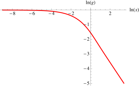
Figure 9: $g(x)$ defined in Eq. (175).

It describes the thermal crossover for $p\ll\Lambda$. More precisely,

$$I_{0}(p,T,\omega=0)=\frac{3\log\left(\frac{\Lambda^{2}}{4p^{2}}\right)+\frac{9}{2}}{128\pi\kappa^{3/2}\sqrt{\rho}}+\frac{3}{16\pi}\frac{T}{\kappa^{2}p^{2}}\,g\!\left(\frac{\omega_{\rm fl}(p)}{8T}\right)+O\Big{(}\frac{p^{2}}{\Lambda^{2}}\Big{)}\quad,\quad\omega_{\rm fl}(p)=p^{2}\sqrt{\kappa/\rho}\ ,$$ (171)

are the first two terms in the expansion in $p/\Lambda$ at fixed $T$. Since this thermal crossover occurs for $p^{2}\sim T\sqrt{\rho/\kappa}$, the formula (171) is useful only for $T\ll T_{\Lambda}=\Lambda^{2}\sqrt{\kappa/\rho}=\omega_{\rm fl}(\Lambda)$, i.e. the Debye temperature for the flexural phonons.

To obtain the small-$T$ behavior we need to expand $g(x)$ at large $x$. For that we note that $4k(k{+}z)+1>1$ in the whole integration domain, hence $\coth(x(4k(k{+}z)+1))$ can be replaced by $1$ at exponential accuracy (i.e. up to $e^{-2x}$) in the the integral (169). By contrast, the term $4k(k{-}z)+1$ in the other argument vanishes for $(z,k)=(1,1/2)$. Expanding around that point and rescaling by defining new variables $z=1-\frac{v}{x}$, $k=\frac{1}{2}+\frac{q}{\sqrt{x}}$, we find at large $x$:

$$g(x)\simeq_{x\to\infty}\frac{C}{x}\quad,\quad C=\int_{0}^{\infty}dv\int_{-\infty}^{\infty}dq\frac{8\sqrt{2}v^{3/2}(\coth(2v+4q^{2})-1)}{3\pi(v+2q^{2})}\approx 0.205617\ .$$ (172)

This yields the low-temperature behavior

$$I_{0}(p,T,\omega=0)=\frac{1}{\kappa^{3/2}\sqrt{\rho}}\bigg{[}\frac{3}{128\pi}\left(\log\left(\frac{\Lambda^{2}}{4p^{2}}\right)+\frac{3}{2}\right)+\frac{3C}{2\pi}\frac{T^{2}}{\omega_{\rm fl}(p)^{2}}+O\left(\frac{p^{2}}{\Lambda^{2}},\frac{T^{3}}{\omega_{\rm fl}(p)^{3}}\right)\bigg{]}.$$ (173)

In the opposite limit of $\omega_{\rm fl}(p)\ll T\ll T_{\Lambda}$, one finds the leading correction to the classical result,

$$I_{0}(p,T,\omega=0)\simeq\frac{3}{16\pi}\frac{T}{\kappa^{2}p^{2}}+\frac{3}{128\pi}\frac{1}{\kappa^{3/2}\sqrt{\rho}}\,\ln\!\left(\frac{\omega_{\rm fl}(p)}{8T}\right),$$ (174)

using that $g(x)\approx_{x\to 0}1+x(\ln x+c)$. Note this is equivalent to the second term in Eq. (171).

For completeness we give the very-high temperature expansion, $T\gg T_{\Lambda}$,

$$I_{0}(p,0)\Big{|}_{\beta\to 0} = \frac{48\Lambda^{4}-p^{4}}{16\beta\pi\kappa^{2}p^{2}(4\Lambda^{2}+p^{2})^{2}}+\frac{\beta^{3}\Lambda^{6}}{23040\pi\rho^{2}}-\frac{\beta^{5}\kappa\Lambda^{6}\left(48\Lambda^{4}+5p^{4}+40\Lambda^{2}p^{2}\right)}{38707200\left(\pi\rho^{3}\right)}$$ (175)

$$+\frac{\beta^{7}\kappa^{2}\Lambda^{6}\left(34560\Lambda^{8}+315p^{8}+5880\Lambda^{2}p^{6}+34608\Lambda^{4}p^{4}+62720\Lambda^{6}p^{2}\right)}{1040449536000\pi\rho^{4}}+O(\beta^{9}).$$

This is not useful for graphene since $T_{\Lambda}=O(3000K)$.

Let us now consider the analytical continuation to real time via $i\omega_{n}\to\omega+i\delta$. The $\omega$-dependent factor in (163) yields the continuation

$${\rm Im}\;\frac{1}{\kappa(4k^{2}+p^{2})^{2}+4\rho\omega_{n}^{2}}\;\to\;\pi\,{\rm sgn}(\omega)\,\delta\!\left(\kappa(4k^{2}+p^{2})^{2}-4\rho\omega^{2}\right)\ .$$ (176)

Calculating the remaining angular integral we obtain

$${\rm Im}\,I_{0}(p,i\omega_{n}\to\omega+i\delta) = \frac{3\rho|\omega|-2p^{2}\sqrt{{\rho}{\kappa}}}{256\kappa^{3/2}\rho^{3/2}\omega}\,\Theta\!\left(\sqrt{\frac{\rho}{\kappa}}|\omega|>p^{2}\right)$$ (177)

$$+\frac{\sqrt{\rho}\left(2|\omega|\sqrt{\frac{\rho}{\kappa}}-p^{2}\right)^{2}\left(2p^{2}-|\omega|\sqrt{\frac{\rho}{\kappa}}\right)}{256\kappa^{5/2}p^{4}\omega\left(\frac{\rho}{\kappa}\right)^{3/2}}\,\Theta\!\left(p^{2}>\sqrt{\frac{\rho}{\kappa}}|\omega|>p^{2}/2\right).$$

This result is presented in the main text in a dimensionless form.

Appendix C Fermion bubble

We recall for completeness the calculation of $J_{0}(p,\omega),$ which is minus the fermion bubble, using free propagators,

$$J_{0}(p,\omega) := -\int\frac{\mathrm{d}^{2}k}{(2\pi)^{2}}\frac{1}{\beta}\sum_{\omega^{\prime}_{n}}\mathrm{tr}\left[\frac{\left(\begin{array}[]{cc}i\omega^{\prime}_{n}+i\omega&-k-p\\ -k^{*}-p^{*}&i\omega^{\prime}_{n}+i\omega\end{array}\right)}{(i\omega^{\prime}_{n}+i\omega)^{2}-|k+p|^{2}}\frac{\left(\begin{array}[]{cc}i\omega^{\prime}_{n}&-k\\ -k^{*}&i\omega^{\prime}_{n}\end{array}\right)}{(i\omega^{\prime}_{n})^{2}-|k|^{2}}\right]$$ (182)

$$= -2\int\frac{\mathrm{d}^{2}k}{(2\pi)^{2}}\frac{1}{\beta}\sum_{\omega^{\prime}_{n}}\frac{k^{2}-\frac{p^{2}}{4}+(i\omega^{\prime}_{n})(i\omega^{\prime}_{n}+i\omega)}{[(i\omega^{\prime}_{n}+i\omega)^{2}-|k+\frac{p}{2}|^{2}][(i\omega^{\prime}_{n})^{2}-|k-\frac{p}{2}|^{2}]}.$$ (183)

Here $\omega\equiv\omega_{m}$ stands for a bosonic Matsubara frequency while $\omega_{n}^{\prime}=\pi(2n+1)/\beta$ is a fermionic one. We have set $v_{\rm F}=1,$ to be restored later. Summing over the $\omega^{\prime}_{n}$ we obtain

$$J_{0}(p,\omega) = -2\int\frac{\mathrm{d}^{2}k}{(2\pi)^{2}}\frac{(k_{-}^{2}-k_{+}^{2})(k_{+}^{2}+k^{2}-\frac{p^{2}}{4})+\omega^{2}(k^{2}-\frac{p^{2}}{4}-k_{+}^{2})}{k_{+}[(k_{+}+k_{-})^{2}+\omega^{2}][(k_{+}-k_{-})^{2}+\omega^{2}]}\tanh\left(\frac{\beta k_{+}}{2}\right)\quad,\quad k_{\pm}=\left|k\pm\frac{p}{2}\right|$$ (184)

$$= \int\frac{\mathrm{d}^{2}k}{(2\pi)^{2}}\frac{2k\cdot p\left(4k^{2}+2k\cdot p+\omega^{2}\right)+p^{2}\omega^{2}}{k_{+}[\omega^{2}\left(4k^{2}+p^{2}+\omega^{2}\right)+4(k\cdot p)^{2}]}\tanh\left(\frac{\beta k_{+}}{2}\right).$$

This can be symmetrized over $p\to-p$. In the limit $T=0$, this reduces to

$$J_{0}(p,\omega)=\int\frac{\mathrm{d}^{2}k}{(2\pi)^{2}}\frac{(k_{+}+k_{-})(k_{+}k_{-}-k^{2}+\frac{p^{2}}{4})}{k_{+}k_{-}[(k_{+}+k_{-})^{2}+\omega^{2}]}\ .$$ (185)

Evaluation of this integral can be done, using distance geometry,

$$\int\frac{\mathrm{d}^{2}k}{(2\pi)^{2}}f(k_{+},k_{-}) = \frac{1}{\pi^{2}}\int\frac{\mathrm{d}k_{+}\,\mathrm{d}k_{-}\,k_{-}k_{+}f(k_{+},k_{-})\Theta(|k_{+}-k_{-}|>p)}{\sqrt{\left(p-k_{-}+k_{+}\right)\left(k_{-}-k_{+}+p\right)\left(k_{-}+k_{+}-p\right)\left(k_{-}+k_{+}+p\right)}}$$ (186)

$$= \frac{1}{4\pi^{2}}\int_{0}^{\infty}\mathrm{d}x\int_{-p/2}^{p/2}\mathrm{d}y\,\frac{(p+x)^{2}-4y^{2}}{\sqrt{x(2p+x)\left(p^{2}-4y^{2}\right)}}f(p+x+y,p+x-y).$$

This gives, restoring the $v_{\rm F}$ factor,

$$J_{0}(p,\omega)=\frac{p^{2}}{16\sqrt{v_{\rm F}^{2}p^{2}+\omega^{2}}}\ .$$ (187)

A similar calculation for arbitrary $\beta$ yields Gazit2

$$J_{0}(p,0)=\frac{T}{\pi v_{\rm F}^{2}}\int_{0}^{1}\mathrm{d}x\,\ln\left(2\cosh\left(\frac{v_{\rm F}\beta p}{2}\sqrt{x(1-x)}\right)\right).$$ (188)

This leads to the classical limit for $v_{\rm F}\beta p\ll 1$,

$$J_{0}(p,0)\simeq\frac{\ln 2}{\pi v_{\rm F}^{2}}T,$$ (189)

and a sharp crossover to $J_{0}(q,0)=p/(16v_{\rm F})$ at $v_{\rm F}\beta p\approx 3$.

Appendix D $O(d)$ symmetry breaking

Although we found in the text that for realistic couplings the instability arises for intermediate wave vectors $q_{c}$, it is still interesting to investigate how an almost uniform order parameter $\sigma(x)\approx\sigma$ and $\alpha(x)\approx\alpha$ could induce a breaking of the $O(d)$ symmetry at a finite $q$ for $h_{1}(x)$.

Smearing out $\sigma(p)$ isotropically around $p=0$, one can replace $\int\sigma(p)P^{\rm T}_{ij}(p)\partial_{i}\partial_{j}\to\left(1-\frac{1}{d}\right)\int\sigma(p)\partial_{i}\partial_{j}.$ Now the saddle-point equation (137) reduces to

$$\kappa k^{4}h_{1}(k)+\frac{k^{2}}{2}\sigma h_{1}(k)=0.$$ (190)

This equation has two solutions, either $h(k)=0$, or the non-trivial solution:

$$h_{1}(k)={\sf h}\delta^{2}(k-k_{0})\ ,$$ (191)

$$\sigma=-2\kappa k_{0}^{2}\ .$$ (192)

This shows that the magnitude of $\sigma(p\approx 0)$ sets a scale for the $O(d)$ symmetry breaking. More investigations are needed to see if a closed solution to the full set of saddle-point equations can be constructed along these lines.

References

- Novoselov et al. (2004) K. S. Novoselov, A. K. Geim, S. V. Morozov, D. Jiang, Y. Zhang, S. V. Dubonos, I. V. Grigorieva, and A. A. Firsov, Science 306, 666 (2004).
- Novoselov et al. (2005) K. S. Novoselov, D. Jiang, F. Schedin, T. J. Booth, V. V. Khotkevich, S. V. Morozov, and A. K. Geim, Proc. Natl. Acad. Sci. U.S.A. 102, 10451 (2005).
- Castro Neto et al. (2009) A. H. Castro Neto, F. Guinea, N. M. R. Peres, K. S. Novoselov, and A. K. Geim, Rev. Mod. Phys. 81, 109 (2009).
- Lee et al. (2008) C. Lee, X. Wei, J. W. Kysar, and J. Hone, Science 321, 5887 (2008).
- Stolyarova et al. (2008) E. Stolyarova, K. T. Rim, S. Ryu, J. Maultzsch, P. Kim, L. E. Brus, T. F. Heinz, M. S. Hybertsen, and G. W. Flynn, Proc. Nat. Ac. Sci. (USA) 104, 9209 (2008).
- Geringer et al. (2009) V. Geringer, M. Liebmann, T. Echtermeyer, S. Runte, M. Schmidt, R. Rückamp, M. C. Lemme, and M. Morgenstern, Phys. Rev. Lett. 102, 076102 (2009).
- Viola Kusminskiy et al. (2011) S. Viola Kusminskiy, D. K. Campbell, A. H. Castro Neto, and F. Guinea, Phys. Rev. B 83, 165405 (2011).
- de Parga et al. (2008) A. L. V. de Parga, F. Calleja, B. Borca, M. C. Passeggi, J. J. Hinarejos, F. Guinea, and R. Miranda, Phys. Rev. Lett. 100, 056807 (2008).
- Meyer et al. (2007) J. C. Meyer, A. K. Geim, M. I. Katsnelson, K. S. Novoselov, T. J. Booth, and S. Roth, Nature 446, 60 (2007).
- Fasolino et al. (2007) A. Fasolino, J. H. Los, and M. I. Katsnelson, Nature Mater. 6, 858 (2007).
- Horovitz and Doussal (2002) B. Horovitz and P. L. Doussal, Phys. Rev. B 65, 125323 (2002).
- Guinea et al. (2008) F. Guinea, B. Horovitz, and P. Le Doussal, Phys. Rev. B 77, 205421 (2008).
- Guinea et al. (2009) F. Guinea, B. Horovitz, and P. Le Doussal, Solid State Communications 149, 1140 (2009).
- Mariani and von Oppen (2008) E. Mariani and F. von Oppen, Phys. Rev. Lett. 100, 076801 (2008).
- Castro et al. (2010) E. V. Castro, H. Ochoa, M. I. Katsnelson, R. V. Gorbachev, D. C. Elias, K. S. Novoselov, A. K. Geim, and F. Guinea, Phys. Rev. Lett. 105, 266601 (2010).
- Mariani and von Oppen (2010) E. Mariani and F. von Oppen, Phys. Rev. B 82, 195403 (2010).
- Gazit (2009a) D. Gazit, Phys. Rev. B 80, 161406 (2009a).
- San-Jose et al. (2011) P. San-Jose, J. González, and F. Guinea, Phys. Rev. Lett. 106, 045502 (2011).
- Gibertini et al. (2012) M. Gibertini, A. Tomadin, F. Guinea, M. I. Katsnelson, and M. Polini, Phys. Rev. B 85, 201405 (2012).
- Nelson and Peliti (1987) D. R. Nelson and L. Peliti, J. Phys. France 48, 1085 (1987).
- Aronovitz and Lubensky (1988) J. A. Aronovitz and T. C. Lubensky, Phys. Rev. Lett. 60, 2634 (1988).
- David and Guitter (1988) F. David and E. Guitter, Europhys. Lett. 5, 709 (1988).
- Le Doussal and Radzihovsky (1992) P. Le Doussal and L. Radzihovsky, Phys. Rev. Lett. 69, 1209 (1992).
- Zakharchenko et al. (2010) K. V. Zakharchenko, R. Roldán, A. Fasolino, and M. I. Katsnelson, Phys. Rev. B 82, 125435 (2010).
- Gonzalez et al. (1994) J. Gonzalez, F. Guinea, and M. A. Vozmediano, Nuclear Physics B 424, 595 (1994).
- Elias et al. (2011) D. C. Elias, R. V. Gorbachev, A. S. Mayorov, S. V. Morozov, A. A. Zhukov, P. Blake, L. A. Ponomarenko, I. V. Grigorieva, K. S. Novoselov, F. Guinea, and A. K. Geim, Nature Physics 7, 701 (2011).
- Vozmediano et al. (2010) M. Vozmediano, M. Katsnelson, and F. Guinea, Physics Reports 496, 109 (2010).
- Ono and Sugihara (1966) S. Ono and K. Sugihara, J. Phys. Soc. Jpn 21, 861 (1966).
- Suzuura and Ando (2002) H. Suzuura and T. Ando, Phys. Rev. B 65, 235412 (2002).
- Choi et al. (2010) S.-M. Choi, S.-H. Jhi, and Y.-W. Son, Phys. Rev. B 81, 081407 (2010).
- Nelson et al. (1989) D. Nelson, T. Piran, and S. W. Eds., Statistical Mechanics of Membranes and Surfaces, Proceedings of the Fifth Jerusalem Winter School for Theoretical Physics (World Scientific, Singapore, 1989).
- (32) K.J. Wiese, in Phase Transitions and Critical Phenomena, C. Domb and J.L. Lebowitz, eds., Acadamic Press London, 1999.
- Wunsch et al. (2006) B. Wunsch, T. Stauber, F. Sols, and F. Guinea, New Journal of Physics 8, 318 (2006).
- Brey and Palacios (2008) L. Brey and J. J. Palacios, Phys. Rev. B 77, 041403 (2008).
- Gazit (2009b) D. Gazit, Phys. Rev. B 79, 113411 (2009b).
- Gazit (2009c) D. Gazit, Phys. Rev. E 80, 041117 (2009c).
- Zinn-Justin (1989) J. Zinn-Justin, Quantum Field Theory and Critical Phenomena (Oxford University Press, Oxford, 1989).
- (38) R. Dillenschneider, Phys. Rev. B 78 115417 (2008)