Composite systems in magnetic field: from hadrons to hydrogen atom

Abstract

We briefly review the recent studies of the behavior of composite systems in magnetic field. The hydrogen atom is chosen to demonstrate the new results which may be experimentally tested. Possible applications to physics of antihydrogen are mentioned.

1 Introduction

We are witnessing an outburst of interest to the behavior of quantum systems in strong magnetic field (MF) [1]. This is probably due to the fact that huge MF up to $eB\sim\Lambda^{2}_{QCD}\sim 10^{19}G$ has become a physical reality. Such field is created (for a short time) in heavy ion collisions at RHIC and LHC [2]. The field about four orders of magnitude less is anticipated to operate in magnetars [3]. It is impossible in a brief presentation to cover the results of intensive studies performed by an impressive number of researches. I concentrate mainly on the work of ITEP group (M. A. Andreichikov B. O. Kerbikov, V. D. Orlovsky, and Yu. A. Simonov). And even more concise on the hydrogen atom in MF problem. The results concerning the quark systems in MF will be merely formulated.

The quantum mechanics of charged particle in magnetic field is presented in textbooks [4]. In a constant MF assumed to be along the $z$ axis the transverse motion is quantized into Landau levels $(\hbar=c=1)$

$$E_{\bot}=\left(n+\frac{1}{2}\right)\omega_{H},~{}~{}n=0,1,2,...,$$ (1)

where $\omega_{H}=\frac{|e|B}{m}$ is the cyclotron frequency. The quantity which in MF takes the role of the mechanical momentum, commutes with the Hamiltonian, and is therefore a constant of motion, is a pseudomomentum [4, 5, 6, 7, 8]

$$\hat{\mbox{\boldmath${\rm K}$}}=\mbox{\boldmath${\rm p}$}-e\mbox{\boldmath${\rm A}$}+e\mbox{\boldmath${\rm B}$}\times\mbox{\boldmath${\rm r}$}=-i\mbox{\boldmath${\rm\nabla}$}-e\mbox{\boldmath${\rm A}$}+e\mbox{\boldmath${\rm B}$}\times\mbox{\boldmath${\rm r}$}.$$ (2)

In the London gauge $\mbox{\boldmath${\rm A}$}(\mbox{\boldmath${\rm r}$})=\frac{1}{2}\mbox{\boldmath${\rm B}$}\times\mbox{\boldmath${\rm r}$}$ the pseudomomentum takes the form

$$\hat{\mbox{\boldmath${\rm K}$}}=\mbox{\boldmath${\rm p}$}+\frac{1}{2}\mbox{\boldmath${\rm B}$}\times\mbox{\boldmath${\rm r}$}.$$ (3)

Mathematically, the conservation of ${\rm K}$ reflects the invariance under the combined action of the spatial translation and the gauge transformation. Physically, ${\rm K}$ is conserved since it takes into account the Lorentz force acting on a particle in MF (motional electric field).

The importance of pseudomomentum becomes clear when we turn to a two-body, or many-body problems in MF.

2 The wave function factorization in MF

The total momentum of $N$ mutually interacting particles with translation invariant interaction is a constant of motion and the center of mass motion can be separated in the Schrodinger equation. For the system with total electric charge $Q=0$ embedded in MF factorization of the wave function can be performed making use of the pseudomomentum operator $\hat{K}$ [5, 6, 7, 8]. As a simple example consider two nonrelativistic particles with masses $m_{1}$ and $m_{2}$, charges $e_{1}=e>0,e_{2}=-e$, and interparticle interaction $V(\mbox{\boldmath${\rm r}$}_{1}-\mbox{\boldmath${\rm r}$}_{2})$. The hydrogen atom is such a system. The Hamiltonian reads

$$\hat{H}=\frac{1}{2m_{1}}(\mbox{\boldmath${\rm p}$}_{1}-e\mbox{\boldmath${\rm A}$}(\mbox{\boldmath${\rm r}$}_{1}))^{2}+\frac{1}{2m_{2}}(\mbox{\boldmath${\rm P}$}_{2}+e\mbox{\boldmath${\rm A}$}(\mbox{\boldmath${\rm r}$}_{2}))^{2}+V(\mbox{\boldmath${\rm r}$}_{1}-\mbox{\boldmath${\rm r}$}_{2}).$$ (4)

Choosing the gauge $\mbox{\boldmath${\rm A}$}=\frac{1}{2}\mbox{\boldmath${\rm B}$}\times\mbox{\boldmath${\rm r}$}$ and introducing

$$M=m_{1}+m_{2},\mu=m_{1}m_{2}(m_{1}+m_{2})^{-1},s=(m_{1}-m_{2})(m_{1}+m_{2})^{-1},$$

$$\mbox{\boldmath${\rm r}$}=\mbox{\boldmath${\rm r}$}_{1}-\mbox{\boldmath${\rm r}$}_{2},\mbox{\boldmath${\rm R}$}=(m_{1}\mbox{\boldmath${\rm r}$}_{1}+m_{2}\mbox{\boldmath${\rm r}$}_{2})M^{-1},\mbox{\boldmath${\rm P}$}=-i\partial/\partial\mbox{\boldmath${\rm R}$},$$

$\mbox{\boldmath${\rm\pi}$}=-i\partial/\partial\mbox{\boldmath${\rm r}$}$, we obtain

$$\hat{H}=\frac{1}{2M}(\mbox{\boldmath${\rm P}$}+\frac{e}{2}\mbox{\boldmath${\rm B}$}\times\mbox{\boldmath${\rm r}$})^{2}+\frac{1}{2\mu}(\mbox{\boldmath${\rm\pi}$}+\frac{e}{2}\mbox{\boldmath${\rm B}$}\times\mbox{\boldmath${\rm R}$}+s\frac{e}{2}\mbox{\boldmath${\rm B}$}\times\mbox{\boldmath${\rm r}$})^{2}.$$ (5)

The two-body pseudomomentum operator is

$$\hat{\mbox{\boldmath${\rm K}$}}=\sum^{2}_{i=1}(\mbox{\boldmath${\rm p}$}_{i}+\frac{1}{2}e_{i}\mbox{\boldmath${\rm B}$}\times\mbox{\boldmath${\rm r}$}_{i})=-i\frac{\partial}{\partial\mbox{\boldmath${\rm R}$}}-\frac{e}{2}\mbox{\boldmath${\rm B}$}\times\mbox{\boldmath${\rm r}$}.$$ (6)

Since $\hat{\mbox{\boldmath${\rm K}$}}$ commutes with $\hat{H},$ the full two-particle wave function $\Psi(\mbox{\boldmath${\rm R}$},\mbox{\boldmath${\rm r}$})$ is the eigenfunction of $\hat{\mbox{\boldmath${\rm K}$}}$ with the eigenvalue ${\rm K}$

$$\hat{\mbox{\boldmath${\rm K}$}}\Psi(\mbox{\boldmath${\rm R}$},\mbox{\boldmath${\rm r}$})=\mbox{\boldmath${\rm K}$}\Psi(\mbox{\boldmath${\rm R}$},\mbox{\boldmath${\rm r}$}),$$ (7)

The wave function which satisfies (7) has the form

$$\psi(\mbox{\boldmath${\rm R}$},\mbox{\boldmath${\rm r}$})=\exp\{(\mbox{\boldmath${\rm K}$}+\frac{e}{2}\mbox{\boldmath${\rm B}$}\times\mbox{\boldmath${\rm r}$})\mbox{\boldmath${\rm R}$}\}\varphi(\mbox{\boldmath${\rm r}$}).$$ (8)

Substitution of the ansatze (8) into $\hat{H}$ leads to the equation

$$\left[\frac{\mbox{\boldmath${\rm K}$}^{2}}{2M}+\frac{e}{M}(\mbox{\boldmath${\rm K}$}\times\mbox{\boldmath${\rm B}$})\mbox{\boldmath${\rm r}$}+\frac{\mbox{\boldmath${\rm\pi}$}^{2}}{2\mu}+\frac{e}{2}\frac{s}{\mu}\mbox{\boldmath${\rm B}$}(\mbox{\boldmath${\rm r}$}\times\mbox{\boldmath${\rm\pi}$})+\frac{e^{2}}{8\mu}(\mbox{\boldmath${\rm B}$}\times\mbox{\boldmath${\rm r}$})^{2}+V(\mbox{\boldmath${\rm r}$})\right]\varphi_{K}(\mbox{\boldmath${\rm r}$})=E\varphi_{K}(\mbox{\boldmath${\rm r}$}).$$ (9)

The subscript $K$ affixed to $E$ reflects the fact that $E$ has a residual dependence on ${\rm K}$ through the second term in (9).

For harmonic interaction $V(\mbox{\boldmath${\rm r}$})=\frac{\sigma^{2}}{m}\mbox{\boldmath${\rm r}$}^{2}$ the problem has an analytical solution and the ground state energy corresponds to $\mbox{\boldmath${\rm K}$}=0$. The simple calculation yields $(m_{1}=m_{2}=m)$

$$E=2\Omega(n_{x}+n_{y}+1)+2\omega(n_{2}+\frac{1}{2})+\frac{1}{4m}\left[\frac{K^{2}_{x}+K_{y}^{2}}{1+\left(\frac{eB}{2\sigma}\right)^{2}}+K^{2}_{z}\right],$$ (10)

$$\Omega=\frac{\sigma}{m}\sqrt{1+\left(\frac{eB}{2\sigma}\right)^{2}},\omega=\frac{\sigma}{m}.$$ (11)

To complete this section, we present examples of the pseudomomentum for three- and four-body systems. Consider a model of the neutron as a system of two $d$-quarks with charges -$e/3$ and masses $m_{d}$, and one $u$-quark with a charge $2e/3$ and a mass $m_{u},M=2m_{d}+m_{u}$. This problem was formulated in Ref. 9 and is now under investigation in relativistic formalism. Following Ref. 9 we introduce the Jacobi coordinates.

$$\mbox{\boldmath${\rm\eta}$}=\frac{\mbox{\boldmath${\rm r}$}_{1}-\mbox{\boldmath${\rm r}$}_{2}}{\sqrt{2}},\mbox{\boldmath${\rm\xi}$}=\sqrt{\frac{m_{u}}{2M}}(\mbox{\boldmath${\rm r}$}_{1}+\mbox{\boldmath${\rm r}$}_{2}-2\mbox{\boldmath${\rm r}$}_{3}),\mbox{\boldmath${\rm R}$}=\frac{1}{M}\sum^{3}_{i=1}m_{i}\mbox{\boldmath${\rm r}$}_{i}.$$ (12)

Then

$$\hat{\mbox{\boldmath${\rm K}$}}=\sum^{3}_{i=1}(\mbox{\boldmath${\rm p}$}_{i}+\frac{1}{2}e_{i}\mbox{\boldmath${\rm B}$}\times\mbox{\boldmath${\rm r}$}_{i})=\mbox{\boldmath${\rm P}$}+\frac{e}{2}\sqrt{\frac{M}{2m_{u}}}\mbox{\boldmath${\rm B}$}\times\mbox{\boldmath${\rm\xi}$}.$$ (13)

As an example of a neutral four-body system consider hydrogen-antihydrogen $H-\bar{H}$ [10]. Let $\mbox{\boldmath${\rm r}$}_{1}$ and $\mbox{\boldmath${\rm r}$}_{2}$ be the coordinates of $p$ and $\bar{p}$, $\mbox{\boldmath${\rm r}$}_{3}$ and $\mbox{\boldmath${\rm r}$}_{4}$ be the coordinates of $e^{-}$ and $e^{+}$. Then

$$\hat{\mbox{\boldmath${\rm K}$}}=\mbox{\boldmath${\rm P}$}+\frac{e}{2}\mbox{\boldmath${\rm B}$}\times\{(\mbox{\boldmath${\rm r}$}_{1}-\mbox{\boldmath${\rm r}$}_{2})+(\mbox{\boldmath${\rm r}$}_{4}-\mbox{\boldmath${\rm r}$}_{3})\}=\mbox{\boldmath${\rm P}$}+\frac{e}{2}\mbox{\boldmath${\rm B}$}\times\{(\mbox{\boldmath${\rm r}$}_{1}-\mbox{\boldmath${\rm r}$}_{3})+(\mbox{\boldmath${\rm r}$}_{2}-\mbox{\boldmath${\rm r}$}_{4})\}.$$ (14)

This obvious result corresponds to the two possible configurations of the system: a)$p\bar{p}+e^{+}e^{-},~{}~{}$ b)$H-\bar{H}.$ Transitions between these two configurations in MF as a Landau–Zener effect will be a subject of a forthcoming publication.

We have reminded the essential formalism needed to treat the composite system under MF. Now we turn to some physical problems.

3 The Hierarchy of MF

The present interest to the effects induced by MF was triggered by the realization of the fact that MF generated in heavy ion collisions reaches the value $eB\sim 10^{19}G\sim\Lambda^{2}_{QCD}$. The highest MF which can be generated now in the laboratory is about $10^{6}G$. From the physical point of view there are two characteristic values of MF strength. The Schwinger one is $B_{cr}=m^{2}_{e}/e=4.414\cdot 10^{13}G$. At $B=B_{cr}$ the distance between the lowest Landau level (LLL) of the electron and the next one is equal to $m_{e}$. This can be seen from (1), or from the relativistic dispersion relation

$$\omega_{n,\sigma}(p_{z})=[p^{2}_{z}+m^{2}+qB(2n+1+\sigma)]^{1/2}.$$ (15)

Here MF is pointing along the $z$-axis, $m$ is the particle mass, $q$ is the absolute value of its electric charge, $\sigma=\pm 1$ depending on the spin projection. The LLL corresponds to $n=0$, $\sigma=-1$. The second important benchmark is the atomic field $B_{a}=m_{e}^{2}e^{3}=2.35\cdot 10^{9}G$. At $B=B_{a}$ the Bohr radius $a_{B}=(\alpha m)^{-1}$ becomes equal to the magnetic, or Landau, radius $l_{H}=(eB)^{-1/2}$, the oscillator energy $eB/2m_{e}$ becomes equal to Rydberg energy $Ry=m_{e}\alpha^{2}/2$. We use the system of units $\hbar=c=1,\alpha=e^{2}=1/137$, dimensionless MF is defined as $H=B/B_{a}$. In this system of units GeV${}^{2}=1.45\cdot 10^{19}G$. The energy to change the electron spin from antiparallel to parallel to B is equal to 2H in units of Rydberg. In terms of $H$ MF is classified [11] as low $(H<10^{-3})$, intermediate, also called strong $(10^{-3}<H<1)$, and intense ($1<H<\infty)$. It seems natural to call MF $eB\sim\Lambda^{2}_{QCD}$ super-intense, and to say that in this region “QED meets QCD” [1].

4 Quarks in super-intense MF: a compendium of the results

A number of papers published on this subject in recent years is of the order of a hundred. Here we present in a very concise form the results of ITEP group (M.A.Andreichikov, B.O.Kerbikov, V.D.Orlovsky and Yu.A.Simonov) [12]. Consider meson or baryon made of quarks embedded in strong MF. There are two parameters defining the transition to the regime when the mass and the geometrical shape of the hadron undergo important changes. The first one is the hadron size $r_{h}\simeq(0.6-0.8)$ fm. The strength of MF corresponding to it is defined by $l_{h}\simeq r_{h}$ which yields $B_{h}\simeq 10^{18}G$. Another related parameter is the string tension $\sigma\simeq 0.18$ GeV² responsible for the confinement. From the condition $eB/\sigma\simeq 1$ we obtain $B_{\sigma}\simeq 10^{19}G$. It is therefore clear that the problem of hadron properties in MF of the order of $(10^{18}-10^{19})G$ has to be formulated and solved at the quark level. The main questions is whether in super-strong MF the hadron mass, e.g., that of the $\rho$- meson, falls down to zero. For the quark system the question is whether MF induces the “fall to the center” phenomenon. It was shown by ITEP group that the answers to both questions are negative.

The relativistic few-body problem is hindered by well-known difficulties. Maybe the most efficient method to solve the problem is the Field-Correlator Method leading to the relativistic Hamiltonian [12]. To elucidate this formalism is beyond the scope of this presentation. The method includes the following steps:

a)

Fock-Feynman-Schwinger proper time representation of the Green’s function.

b)

Derivation of the confinement and OGE (color Coulomb) interactions using minimal surface Wilson loop.

c)

Introduction of the quark dynamical masses (einbein formalism).

d)

Inclusion of the spin-dependent interactions ${\rm\sigma}$${\rm B}$ and hyperfine.

e)

Derivation of the relativistic Hamiltonian $\hat{H}$ as the end-result of a)-d).

f)

Determination of the hadron mass and wave function

At step b) one obtains the confinement interaction in the form $\sigma|\mbox{\boldmath${\rm r}$}_{i}-\mbox{\boldmath${\rm r}$}_{j}|$ with $\sigma$ being the string tension. In order to obtain analytical and physically transparent results we replaced the linear potential according to

$$V_{conf}=\sigma r\to\frac{\sigma}{2}\left(\frac{r^{2}}{\gamma}+\gamma\right),$$ (16)

where $\gamma$ is a variational parameter. Minimizing (16) with respect to it, one retrieves the original form of $V_{conf}$. As was shown by the numerical calculations, the accuracy of this procedure is $\mathrel{\mathchoice{\lower 3.6pt\vbox{\halign{$\mathsurround=0pt\displaystyle\hfil#\hfil$\cr<\crcr\sim\crcr}}}{\lower 3.6pt\vbox{\halign{$\mathsurround=0pt\textstyle\hfil#\hfil$\cr<\crcr\sim\crcr}}}{\lower 3.6pt\vbox{\halign{$\mathsurround=0pt\scriptstyle\hfil#\hfil$\cr<\crcr\sim\crcr}}}{\lower 3.6pt\vbox{\halign{$\mathsurround=0pt\scriptscriptstyle\hfil#\hfil$\cr<\crcr\sim\crcr}}}}5\%$. With the account of MF and confinement, but without spin-dependent terms, the hamiltonian has the form

$$\hat{H}_{q\bar{q}}=\frac{1}{\omega}\left(-\frac{\partial^{2}}{\partial\mbox{\boldmath${\rm r}$}^{2}}+\frac{e^{2}}{4}(\mbox{\boldmath${\rm B}$}\times\mbox{\boldmath${\rm r}$})^{2}\right)+\frac{\sigma}{2}\left(\frac{r^{2}}{\gamma}+\gamma\right).$$ (17)

This is a two-oscillator problem similar to (10)-(11). We are focusing on the ground state, hence the pseudomomentum can be taken equal to zero (see (11)), and it does not enter into (17). We note in passing that in the relativistic Hamiltonian approach we evade a subtle problem of the center-of-mass of the relativistic system. The mass eigenvalue $M(\omega)$ and the dynamical mass $\omega$ are determined from a set of equations.

$$\hat{H}\psi=M(\omega)\psi,~{}~{}\frac{\partial M(\omega)}{\partial\omega}=0.$$ (18)

The wave function which is a solution of (18) with the Hamiltonian (17) is

$$\Psi(\mbox{\boldmath${\rm r}$})=\frac{1}{\sqrt{\pi^{3/2}a^{2}_{\bot}a_{z}}}\exp\left(-\frac{r^{2}_{\bot}}{2a^{2}_{\bot}}-\frac{r^{2}_{z}}{2a^{2}_{z}}\right),$$ (19)

where at $eB\gg\sigma$ one has $a_{\bot}\simeq\sqrt{\frac{2}{eB}},~{}~{}a_{z}\simeq\frac{1}{\sqrt{\sigma}}$. With MF increasing the $q\bar{q}$ system acquires the form of an elongated ellipsoid, see Fig. 1.

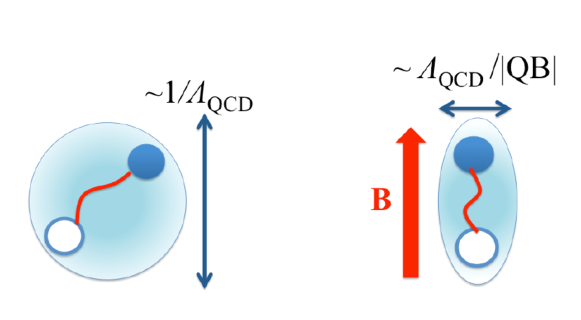
Figure 1: A sketch of MF influence on the meson wave function (from Ref. 13).

A similar behavior was observed before for the hydrogen atom in strong MF [14]. The difference is that the longitudinal size of the $q\bar{q}$-meson is bounded by $a_{z}\sim 1/\sqrt{\sigma}$ in contrast to the hydrogen atom which in a strong MF takes the needlelike form with $a_{z}\sim(\ln H)^{-1}$.

The contribution of $V_{OGE}$ (color Coulomb) was calculated as the average value of $V_{OGE}$ over the wave function (19) with quark and gluon loop corrections taken into account. Hyperfine (hf) spin-spin interaction was treated in a similar way. Here a special care should be devoted to the $\delta$-function. Taken literally, it would lead to a divergent $\psi^{2}(0)\sim eB$ factor (see the next section). Therefore the $\delta$-function was smeared over the radius $\sim 0.2$ fm.

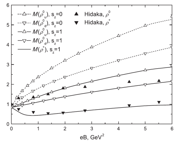
Figure 2: The results of the calculations of the $\rho$- meson mass as a function of MF strength together with the lattice data [15].

In Fig. 2 the results for the $\rho$-meson mass as a function of MF strength ar presented together with the lattice data [15]. We remind that MF violates both spin and isospin symmetries. In order to minimize the Zeeman energy the lowest state of $u\bar{u}$ (or $d\bar{d}$) in strong MF becomes spin polarized $|u\uparrow\bar{u}\downarrow\rangle$. In our somewhat oversimplified picture this state is a mixture of $\rho^{0}$ and $\pi^{0}$. The conclusion is that the mass of the quark-antiquark state does not reach zero no matter now strong MF is. The same result is true for the neutron made of three quarks.

Here we covered only few results of ITEP group on quarks in MF — see Ref. 12.

5 The new results on Zeeman levels in hydrogen

The spectrum of hydrogen atom (HA) in MF is a classical problem described textbooks [4]. The present wave of interest to superstrong MF inspired the reexamination of this problem [16, 17, 18, 19]. Surprisingly enough, the new important results were obtained. It was shown that in superstrong MF radiative corrections screen the Coulomb potential thus leading to the freezing of the ground state energy at the value $E_{0}=-1.7$ keV [18, 19].

Here we discuss the new correction to hyperfine (hf) splitting in HA [14]. In HA the dramatic changes of the ground state binding energy and the wave function geometry occurs starting from $H\simeq 1$. In this region magnetic confinement in the plane perpendicular to MF dominates the Coulomb binding to the proton. With MF strength growing, the binding energy rises [16, 17, 18, 19]. The wave function squeezes and takes the needlelike form. The probability to find the electron near the proton increases. This means that the value of the wave function at the origin $|\psi(0)|^{2}$ depends on MF and in the limit $H\gg 1$ one has $|\psi(0)|^{2}\sim H\ln H$ [14]. This phenomenon may be called “Magnetic Focusing of Hyperfine Interaction in Hydrogen”. In addition, the deviation of the HA ground state wave function from the spherical symmetry results in the appearance of the tensor forces. These two MF induced effects result in corrections to the standard picture (see Fig. 3) of the Zeeman splitting. The energies of the splitted levels are found by the diagonalization of the following Hamiltonian [14]

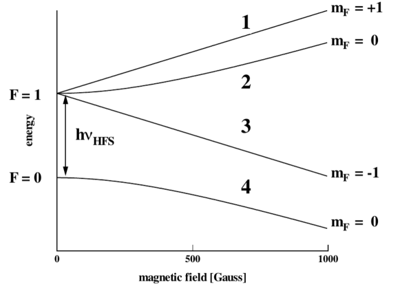
Figure 3: Hydrogen hf structure. Transition $|2\rangle\to|4\rangle$ at $B=0$ corresponds to the $\lambda=21$ cm (1420 MHz) line.

$$\hat{H}_{hf}=\frac{8\pi}{3}g\mu_{B}\mu_{N}|\psi_{B}(0)|^{2}\mbox{\boldmath${\rm\sigma}$}_{e}\mbox{\boldmath${\rm\sigma}$}_{p}+\frac{8\pi}{3}\delta\psi_{B}(0)\sigma_{ez}\sigma_{pz}+\mu_{B}(\mbox{\boldmath${\rm\sigma}$}_{e}\mbox{\boldmath${\rm B}$})-g\mu_{N}(\mbox{\boldmath${\rm\sigma}$}_{p}\mbox{\boldmath${\rm B}$}).$$ (20)

Here $g=2.79,g\mu_{n}$ is the proton magnetic moment, $\mu_{B}$ is the Bohr magneton, index $B$ affixed to $\psi_{B}$ and $\delta\psi_{B}$ indicates the dependence on MF. At $B=0$ one retrieves the standard expression with $|\psi_{B}(0)|^{2}=m^{3}\alpha^{3}/\pi$ and $\delta\psi_{B}(0)=0$. We do not discuss the corrections to the $\Delta E_{hf}=1420MHz$ line due to relativistic effects, QED, and nuclear structure. This subject is thoroughly elucidated in the literature [20, 21]. For the frequency of the $\Delta F=1,\Delta m_{F}=0~{}~{}|2>\to|4>$ transition diagonalization of the Hamiltonian (19) yields

$$\nu=E_{2}-E_{4}=\Delta E_{hf}\sqrt{\gamma^{2}+\left(\frac{2\mu_{B}B}{\Delta E_{hf}}\right)^{2}\left(1+g\frac{m_{e}}{m_{p}}\right)^{2}}.$$ (21)

Here $\gamma^{2}$ is a new MF dependent parameter with the following asymptotic behavior [14].

$$\gamma\to 1+\left(1-\frac{a^{2}_{\bot}}{a^{2}_{z}}\right),~{}~{}H\ll\alpha^{2}\frac{m_{e}}{m_{p}}\simeq 10^{-7},$$ (22)

$$\gamma\to H\ln H,~{}~{}H\gg 1,$$ (23)

$$\gamma\gg\frac{2\mu_{B}B}{\Delta E_{nf}},~{}~{}\ln H\gg 10^{7}.$$ (24)

In the standard picture without magnetic focusing $\gamma\equiv 1$.

The question is whether magnetic focusing in HA can be experimentally detected in the laboratory conditions. A very preliminary positive answer relies on extremely accurate experiments in search of Zeeman frequency variation using the hydrogen maser [22]. It typically operates with constant MF of the order of $\sim 1$ mG. In this regime the frequencies of the $F=1,\Delta m_{F}=\pm 1$ Zeeman transitions were measured with a precision of $\sim 1$ mHz [22]. This subject deserves a detailed discussion to be presented in another publication.

This presentation is based on the work of the ITEP team: M. A. Andreichikov, B. K., V. D. Orlovsky and Yu. A. Simonov.

The author gratefully acknowledges the encouraging discussions with M. I. Vysotsky, S. I. Godunov, V. S. Popov, B. M. Karnakov, A. E. Shabad and A. Yu. Voronin.

References

- [1] D. E. Kharzeev, K. Landsteiner, A. Schmitt, and H.-U. Yee, Lect. Notes Phys. 871, 1 (2013).
- [2] D. E. Kharzeev, L. D. McLerran and H. J. Warringa, Nucl. Phys.A 803, 227 (2008); V. Skokov, A. Illarionov and V. Toneev, Int. J. Mod. Phys.A 24, 5925 (2009).
- [3] A. Y. Potekhin, Phys. Usp. 53, 1235 (2010); A. K. Harding and Dong Lai, Rept. Prog. Phys. 69, 2631 (2006).
- [4] L. D. Landau and E. M. Lifshitz, Quantum mechanics. Course of Theoretical Physics, vol. 3, Pergamon Press, Oxford (1978).
- [5] W. E. Lamb, Phys. Rev. 85, 259 (1952); L. P. Gor’kov and I. E. Dzyaloshinskii, Soviet Physics JETP, 26, 449 (1968); J. E. Avron, I. W. Herbst, and B. Simon, Ann. Phys. (NY), 114, 431 (1978); H. Grotsch and R. A. Hegstrom, Phys. Rev. A 4, 59 (1971).
- [6] H. Herold, H. Ruder, and G. Wunner, J. of Phys. B 14, 751 (1981).
- [7] Dong Lai, Rev. Mod. Phys. 73, 629 (2001).
- [8] J. Alford and M. Strickland, Phys. Rev. D 88, 105017 (2013).
- [9] Yu. A. Simonov, Phys. Lett. B 719, 464 (2012).
- [10] A. Yu. Voronin and P. Froelich, Phys. Rev. A 77, 022505 (2008).
- [11] M. D. Jones, G. Ortiz, and D. M. Ceperley, Phys. Rev. A 54, 219 (1996).
- [12] M. A. Andreichikov, B. O. Kerbikov, V. D. Orlovsky, and Yu. A. Simonov, Phys. Rev. D 87, 094029 (2013); M. A. Andreichikov, V. D. Orlovsky, and Yu. A. Simonov, Phys. Rev. Lett. 110, 162002 (2013); V. D. Orlovsky and Yu. A. Simonov, JHEP 1309, 136 (2013), arXiv:1306.2232 [hep-ph]; Yu. A. Simonov, Phys. Rev. D 88, 025028 (2013), arXiv:1303.4952 [hep-ph]; M. A. Andreichikov, B. O. Kerbikov, Yu. A. Simonov, arXiv:1304.2516 [hep-ph];Yu. A. Simonov, arXiv:1308.5553 [hep-ph]; Yu. A. Simonov, Phys. Rev. D 88, 053004 (2013).
- [13] Toru Kojo and Nan Su, The quark mass gap in a magnetic field, arXiv:1211.7318 [hep-ph].
- [14] M. A. Andreichikov, B. O. Kerbikov, and Yu. A. Simonov, Magnetic field focussing of hyperfine interaction in hydrogen, arXiv:1304.2516 [hep-ph].
- [15] Y. Hidaka and A. Yamamoto, Phys. Rev. D 87, 094502 (2013).
- [16] B. M. Karnakov, V. S. Popov, J. Exp. Theor. Phys. 114, 1 (2012); Physics uspekhi, accepted for publication.
- [17] A. E. Shabad and V. V. Usov, Phys. Rev. Lett. 98, 180403 (2007); Phys. Rev. D 77, 025001 (2008).
- [18] B. Machet and M. I. Vysotsky, Phys. Rev. D 83, 025022 (2011).
- [19] S. I. Godunov, B. Machet, M. I. Vysotsky, Phys. Rev. D 85, 044058 (2012).
- [20] S. G. Karshenboim, Phys. Rept., 422, 1 (2005).
- [21] M. I. Eides, H. Grotch, and V. A. Shelyuto, Phys. Rept., 342, 63 (2001).
- [22] D. F. Phillips et al., Phys. Rev. D 63, 111101 (2001); M. A. Humphrey et al., Phys. Rev. A 68, 063807 (2003).