A new angular momentum method for
computing wave maps into spheres

Abstract.

In this paper, we present and analyze a new finite difference method for computing three dimensional wave maps into spheres. By introducing the angular momentum as an auxiliary variable, we recast the governing equation as a first order system. For this new system, we propose a discretization that conserves both the energy and the length constraint. The new method is also fast requiring only $N\log N$ operations at each time step. Our main result is that the method converges to a weak solution as discretization parameters go to zero. The paper is concluded by numerical experiments demonstrating convergence of the method and its ability to predict finite time blow-up.

1. Introduction

The purpose of this paper is to develop a new numerical method for computing wave maps. By wave maps, we here mean vectors $d=[d_{1},d_{2},d_{3}]^{T}$ satisfying the following constrained wave equation:

$$\begin{split}d_{tt}-\Delta d&=\gamma d,\quad|d|=1,\quad\text{ in $(0,\infty)\times\Omega$}.\end{split}$$ (1.1)

Here, $\Omega\subset\mathbb{R}^{n}$, $n=2,3$, is either assumed to be the unit box $\Omega=[0,1]^{n}$ or it is assumed that $\Omega=\mathbb{T}^{n}$, where $\mathbb{T}^{n}$ is the n-dimensional torus. In the first case, (1.1) is augmented with homogenous Neumann boundary conditions.

The $\gamma$ appearing in (1.1) is a Lagrange multiplier enforcing the constraint $|d|=1$. In particular, by dotting (1.1) with $d$ and using that $|d|=1$, one finds that

$$\gamma=|\nabla d|^{2}-|d_{t}|^{2}.$$

Thus, (1.1) is in this sense highly nonlinear which in turn obscures the task of developing conservative numerical methods. Moreover, in three spatial dimensions, it is known that solutions of (1.1) may blow-up [5]. Specifically, there is initial data for which the gradient $\nabla d$ develops singularities in finite time. Thus, solutions of the wave map equation are not smooth. We will return to the issue of blow-up in the numerical section (Section 5).

The literature on numerical methods for (1.1) seems to be confined to a handful of results. In the papers [1, 3, 4], the authors develops convergent splitting and relaxation methods. With these methods, (1.1) is either solved iteratively, using one evolution step and one projection step onto the sphere, or the constraint $|d|=1$ is relaxed altogether. In the paper [2], the wave map equation (1.1) is computed using an approximate Lagrange multiplier $\gamma_{h}$. The approximate $\gamma_{h}$ is then designed such that the constraint $|d|=1$ holds. Clearly, this leads to a $\gamma_{h}$ which depends nonlinearly and implicit on the unknown $d$ and hence leads to a rather unpractical method.

The method we will develop in this paper differs significantly from the previously proposed methods. The key observation allowing us to deduce an energy and constraint preserving method is a new formulation of (1.1). Specifically, by introducing the angular momentum:

$$w=d_{t}\times d.$$

the wave map equation (1.1) can be recast in the form

$$d_{t} =d\times w,$$ (1.2)

$$w_{t} =\Delta d\times d.$$ (1.3)

In this formulation, the constraint $|d|=1$ is inherit and hence there is no need for the Lagrange multiplier $\gamma$. Constraint preserving time integration for this system is easily derived. Here, we will use the first order integration:

$$\begin{split}\frac{d^{m+1}-d^{m}}{\Delta t}&=w^{m+1/2}\times d^{m+1/2}\\ \frac{w^{m+1}-w^{m}}{\Delta t}&=\Delta d^{m+1/2}\times d^{m+1/2},\end{split}$$ (1.4)

where $d^{m+1/2}=\frac{1}{2}(d^{m}+d^{m+1})$ and similarly $w^{m+1/2}=\frac{1}{2}(w^{m}+w^{m+1})$. This integration method satisfies $|d^{m+1}|=|d^{m}|$. Moreover, by dotting the second equation with $w^{m+1/2}$ and adding the first equation dotted with $\Delta d^{m+1/2}$, one obtains

$$\int_{\Omega}|w^{m+1}|^{2}+|\nabla d^{m+1}|^{2}~{}dx=\int_{\Omega}|w^{m}|^{2}+|\nabla d^{m}|^{2}~{}dx,$$

and hence the method also conserves the energy. To discretize (1.4) in space, we will use a standard central difference approximation of the Laplace operator on a regular grid.

The only potential downside of using the discretization (1.4) is that it is nonlinear and implicit and hence requires implementing a fixed point solver. Moreover, this fixed point solver should be such that at least the length constraint is conserved at every iteration. In Section 4, we will give the details on how such a solver may be constructed and prove that a fixed point may be computed (up to any tolerance in energy norm) using only $N\log N$ operations, where $N$ is the number of degrees of freedom of $d$. In practice, finding a solution with tolerance $N^{-2}$ requires only around $5-10$ iterations depending on the regularity of the underlying solution, but not on $N$. Note that there is not much point in decreasing the tolerance beyond $N^{-2}$ as the discretization error of (1.4) will then dominate the error.

Our main theoretical result in this paper is that the new angular momentum method converges to a weak solution as discretization parameters go to zero. The proof of this fact will follow directly using energy arguments together with the observation that

$$\Delta d\times d=\operatorname{div}(A(d)\nabla d),$$

for some matrix $A$.

The remaining parts of this paper are structured as follows: In the upcoming section, we will properly define the new method and prove some basic properties. Then, in Section 3, we will prove that the method converges to a weak solution as discretization parameters go to zero. In Section 4, we will provide a way to compute the needed fixed point through an iterative procedure and prove that a fixed point may be obtained using only $N\log N$ operations. In Section 5, the paper is concluded by a series of numerical experiments illuminating some of the properties of the new method.

2. The angular momentum method

Given a number of degrees of freedom $N$, we set $M=N^{\frac{1}{n}}$, where $n=2$, $3$ is the spatial dimension, and assume that $M$ is an integer. Next, we let $h=1/M$ and set the time step $\Delta t=\kappa h$, where $\kappa$ is some constant. The domain $\Omega$ is then discretized in terms of the $N$ points

$$x_{i,j,k}=(ih,jh,kh),\quad i,j,k=0,\ldots,M.$$

To simplify notation, we introduce the multiindex $\underline{i}\in\mathcal{I}_{N}:=\{0,\dots,M\}^{3}$ such that we can write

$$x_{\underline{i}}=x_{i,j,k}.$$

We will approximate $d$ at these points. Specifically,

$$d^{m}_{\underline{i}}\approx d(m\Delta t,x_{\underline{i}}).$$

Next, let $\mathbb{1}:=(1,0,0)$, $\mathbb{2}:=(0,1,0)$, and $\mathbb{3}:=(0,0,1)$. Using these vectors, we then define the forward and backward difference operators

$$D^{+}_{j}d_{\underline{i}}=\frac{d_{\underline{i}+\mathbbm{j}}-d_{\underline{i}}}{h},\qquad D^{-}_{j}d_{\underline{i}}=D^{+}_{j}d_{\underline{i}-\mathbbm{j}}$$

respectively, for $j=1,2,3$, and $\underline{i}\in\mathcal{I}_{N}$. The standard central Laplace discretization is then defined as

$$\Delta_{h}d_{\underline{i}}=\sum_{j=1}^{3}D_{j}^{+}D_{j}^{-}d_{\underline{i}}.$$

If we introduce the backward gradient $\nabla_{h}=[D^{-}_{1},D^{-}_{2},D^{-}_{3}]^{T}$ and forward divergence $\operatorname{div}_{h}v=D^{+}_{1}v^{(1)}+D^{+}_{2}v^{(2)}+D^{+}_{3}v^{(3)}$, we have the identity

$$\operatorname{div}_{h}\nabla_{h}=\Delta_{h},$$

which will be convenient in the upcoming analysis.

For time discretization, we will use the notation

$$d^{m+1/2}:=\frac{d^{m}+d^{m+1}}{2},\quad D_{t}d^{m}=\frac{d^{m+1}-d^{m}}{\Delta t}.$$

To approximate the initial conditions, we shall use the operator

$$\Pi[f]_{\underline{i}}=\frac{1}{(h)^{3}}\int_{(i-0.5)h}^{(i+0.5)h}\int_{(j-0.5)h}^{(j+0.5)h}\int_{(k-0.5)h}^{(k+0.5)h}f(y)~{}dy,$$

with the obvious modification if $d=2$.

We are now ready to state the new method.

Definition 2.1.

Given initial data $d^{0}\in H^{1}(\Omega)$, $d^{0}_{t}\in L^{2}(\Omega)$, let $$(d^{0}_{\underline{i}},~{}w^{0}_{\underline{i}})=\left(\Pi[d^{0}]_{\underline{i}},\Pi[d_{t}^{0}\times d^{0}]_{\underline{i}}\right),\quad\forall\underline{i}.$$ Determine sequentially, $$d^{m}_{\underline{i}},w^{m}_{\underline{i}},\qquad\forall\underline{i}\in\mathcal{I}_{N},\quad m=1,\ldots,$$ by solving the nonlinear system $\displaystyle D_{t}d_{\underline{i}}^{m}$ $\displaystyle=d_{\underline{i}}^{m+1/2}\times w_{\underline{i}}^{m+1/2},$ (2.1) $\displaystyle D_{t}w_{\underline{i}}^{m}$ $\displaystyle=\Delta_{h}d_{\underline{i}}^{m+1/2}\times d_{\underline{i}}^{m+1/2}.$ (2.2)

We will now prove some fundamental properties of the new method.

Lemma 2.2.

There exists a unique numerical solution to the method posed in Definition 2.1. Moreover, the length is preserved

$$|d_{i}^{m}|=|d_{i}^{0}|=1,\quad\forall i,\quad m=0,\ldots,$$ (2.3)

and the energy is preserved

$$E_{m}=E_{0},\quad m=1,\ldots,$$ (2.4)

where the energy is defined as

$$E_{m}=\frac{1}{2}\int_{\Omega}|\nabla_{h}d^{m}_{h}|^{2}+|w^{m}_{h}|^{2}\,dx.$$ (2.5)

Proof.

The existence of a unique solution will be proved through a constructive iteration in Section 4. The proof can be found in Corollary 4.9.

That the length is conserved, (2.3), follows immediately from (2.1). Indeed, dotting with $d^{m+1/2}_{h}$ yields

$$D_{t}d_{h}^{m}\cdot d_{h}^{m+1/2}=0.$$

Finally, to prove (2.4), we calculate

$$\begin{split}D_{t}E_{m}&=\int_{\Omega}w^{m+1/2}\cdot D_{t}w^{m}-\Delta_{h}d^{m+1/2}\cdot D_{t}d^{m}~{}dx\\ &=\int_{\Omega}\left(\Delta_{h}d^{m+1/2}\times d^{m+1/2}\right)\cdot w^{m+1/2}~{}dx\\ &\qquad-\int_{\Omega}\left(d^{m+1/2}\times w^{m+1/2}\right)\cdot\Delta_{h}d^{m+1/2}~{}dx=0.\end{split}$$

This concludes the proof. ∎

3. The method converges

To prove that the method converges, it will be convenient to extend the numerical solution to all of $\Omega$. For this purpose, we shall use the piecewise constant extension:

$$\begin{split}d^{m}_{h}(x)&=d_{\underline{i}}^{m},\quad x\in E_{\underline{i}},\\ w^{m}_{h}(x)&=w_{\underline{i}}^{m},\quad x\in E_{\underline{i}},\end{split}$$ (3.1)

where $E_{\underline{i}}=[(i-1/2)h,(i+1/2)h)\times[(j-1/2)h,(j+1/2)h)\times[(k-1/2)h,(k+1/2)h)$, $\underline{i}=(i,j,k)\in\mathcal{I}_{N}$. Observe that the numerical method can then be written

$$D_{t}d^{m}_{h} =d^{m+1/2}_{h}\times w_{h}^{m+1/2},$$ (3.2)

$$D_{t}w_{h}^{m} =\Delta_{h}d_{h}^{m+1/2}\times d^{m+1/2}_{h},$$ (3.3)

where $\Delta_{h}$ is derived in the obvious way.

Our main result in this section is the following convergence result:

Theorem 3.1.

Let $\{(d_{h},w_{h})\}_{h>0}$ be a sequence of numerical approximations obtained using Definition 2.1 and (3.1), where $\Delta t=\kappa h$ for some constant $\kappa>0$. Then, as $h\rightarrow 0$, $d_{h}\rightarrow d$ a.e and in $L^{p}((0,\infty)\times\Omega)$ for any $p<\infty$, $w_{h}\overset{\star}{\rightharpoonup}w$ in $L^{\infty}(0,T;L^{2}(\Omega))$, where $(d,w)$ is a weak solution of the wave map equation (1.2)–(1.3). By a weak solution, we mean that $(d,w)$ satisfies

$$\begin{split}\int_{0}^{\infty}\int_{\Omega}d\phi_{t}+(d\times w)\phi~{}dxdt+\int_{\Omega}d^{0}\phi(0,\cdot)\,dx&=0,\\ \int_{0}^{\infty}\int_{\Omega}w\psi_{t}+(d\times\nabla^{T}d):\nabla^{T}\psi~{}dxdt+\int_{\Omega}w^{0}\psi(0,\cdot)\,dx&=0,\end{split}$$ (3.4)

for all $\phi,\psi\in C^{\infty}_{0}([0,\infty)\times\Omega;\mathbb{R}^{n})$, where the supscript $T$ means the transposed gradient matrix.

To prove this theorem, our starting point is Lemma 2.2 yielding the $h$-independent bounds:

$$\begin{split}D_{t}d_{h}&\in_{b}L^{\infty}(0,\infty;L^{2}(\Omega)),\\ \nabla_{h}d_{h}&\in_{b}L^{\infty}(0,\infty;L^{2}(\Omega)),\\ w_{h}&\in_{b}L^{\infty}(0,\infty;L^{2}(\Omega)),\end{split}$$

where the $\in_{b}$ means that the inclusion is independent of $h$. From these bounds, we can assert the existence of functions $d$ and $w$, and a subsequence $h_{j}$, such that

$$\begin{split}w_{h}&\overset{\star}{\rightharpoonup}w\text{ in $L^{\infty}(0,\infty;L^{2}(\Omega))$},\\ D_{t}d_{h}&\overset{\star}{\rightharpoonup}d_{t}\text{ in $L^{\infty}(0,\infty;L^{2}(\Omega))$},\\ \nabla_{h}d_{h}&\overset{\star}{\rightharpoonup}\nabla d\text{ in $L^{\infty}(0,\infty;L^{2}(\Omega))$},\\ d_{h}&\rightarrow d\text{ a.e and in $L^{p}((0,\infty)\times\Omega)$ for $p<\infty$},\end{split}$$ (3.5)

where the limit $d$ also satisfies the constraint

$$|d(t,x)|=1\text{ a.e in $[0,\infty)\times\Omega$}.$$

To show that the limit pair $(d,w)$ is a weak solution of (1.2) – (1.3), we will need a vector identity. It is this identity which allows us to pass to the limit without having higher-order bounds on $d$.

Lemma 3.2.

The following identity holds,

$$\begin{split}d_{h}\times\Delta_{h}d_{h}&=\operatorname{div}_{h}\begin{pmatrix}d_{h}^{(2)}\nabla_{h}^{T}d_{h}^{(3)}-d_{h}^{(3)}\nabla_{h}^{T}d_{h}^{(2)}\\ d_{h}^{(3)}\nabla_{h}^{T}d_{h}^{(1)}-d_{h}^{(1)}\nabla_{h}^{T}d_{h}^{(3)}\\ d_{h}^{(1)}\nabla_{h}^{T}d_{h}^{(2)}-d_{h}^{(2)}\nabla_{h}^{T}d_{h}^{(1)}\end{pmatrix}.\end{split}$$ (3.6)

Proof.

By direct calculation, we see that

$$d^{(k)}_{\underline{i}}\,\Delta_{h}d_{\underline{i}}^{(\ell)}=\operatorname{div}_{h}\left(d^{(k)}_{\underline{i}}\nabla_{h}d_{\underline{i}}^{(\ell)}\right)-\nabla_{h}d_{\underline{i}}^{(\ell)}\cdot\nabla_{h}d_{\underline{i}}^{(k)},$$

for $k,\ell\in\{1,2,3\}$. Hence

$$d^{(k)}_{\underline{i}}\,\Delta_{h}d_{\underline{i}}^{(\ell)}-d^{(\ell)}_{\underline{i}}\,\Delta_{h}d_{\underline{i}}^{(k)}=\operatorname{div}_{h}\left(d^{(k)}_{\underline{i}}\nabla_{h}d^{(\ell)}_{\underline{i}}-d^{(\ell)}_{\underline{i}}\nabla_{h}d^{(k)}_{\underline{i}}\right)$$

and (3.6) follows. ∎

3.1. Proof of Theorem 3.1:

For test functions $\varphi$, $\psi\in C^{1}_{0}([0,\infty)\times\Omega;\mathbb{R}^{n})$, we denote $\varphi^{m}(x):=\varphi(t^{m},x)$, $\psi^{m}(x):=\psi(t^{m},x)$. Then we dot (3.2) and (3.3) with $\varphi^{m},\psi^{m}$, integrate over $\Omega$, and sum over $m$, to discover

$$\Delta t\sum_{m=0}^{\infty}\int_{\Omega}\left(D_{t}d^{m}_{h}-d^{m+1/2}_{h}\times w_{h}^{m+1/2}\right)\cdot\varphi^{m}\,dx =0,$$

$$\Delta t\sum_{m=0}^{\infty}\int_{\Omega}\left(D_{t}w_{h}^{m}+d^{m+1/2}_{h}\times\Delta_{h}d_{h}^{m+1/2}\right)\cdot\psi^{m}\,dx =0.$$

Using Lemma 3.2 and summation by parts, we deduce that

$$\begin{split}\Delta t\sum_{m=0}^{\infty}\int_{\Omega}\left(-d^{m+1}_{h}\cdot D_{t}\varphi^{m}-\left(d^{m+1/2}_{h}\times w_{h}^{m+1/2}\right)\cdot\varphi^{m}\right)dx\quad&\\ -\int_{\Omega}d^{0}_{h}\cdot\varphi^{0}\,dx&=0,\\ \Delta t\sum_{m=0}^{\infty}\int_{\Omega}\left(-w_{h}^{m+1}\cdot D_{t}\psi^{m}-\left(d^{m+1/2}_{h}\times\nabla_{h}^{T}d_{h}^{m+1/2}\right):\nabla_{h}^{T}\psi^{m}\right)dx\quad&\\ -\int_{\Omega}w^{0}_{h}\cdot\psi^{0}\,dx&=0,\end{split}$$ (3.7)

We denote

$$\begin{split}d_{h}(t,x)&=d_{h}^{m}(x),\quad x\in\Omega,\quad t\in(t^{m-1},t^{m}],\\ w_{h}(t,x)&=w_{h}^{m}(x),\quad x\in\Omega,\quad t\in(t^{m-1},t^{m}],\\ \overline{d}_{h}(t,x)&=d_{h}^{m-1/2}(x),\quad x\in\Omega,\quad t\in(t^{m-1},t^{m}],\\ \overline{w}_{h}(t,x)&=w_{h}^{m-1/2}(x),\quad x\in\Omega,\quad t\in(t^{m-1},t^{m}],\\ \end{split}$$

such that (3.7) becomes

$$\begin{split}-\int_{0}^{\infty}\int_{\Omega}\left(d_{h}\cdot D_{t}\varphi+\left(\overline{d}_{h}\times\overline{w}_{h}\right)\cdot\varphi\right)\,dx\,dt-\int_{\Omega}d_{h}^{0}\cdot\varphi(0,\cdot)\,dx&=0,\\ -\int_{0}^{\infty}\int_{\Omega}\left(w_{h}\cdot D_{t}\psi+\left(\overline{d}_{h}\times\nabla_{h}^{T}\overline{d}_{h}\right):\nabla_{h}^{T}\psi\right)\,dx-\int_{\Omega}w_{h}^{0}\cdot\psi(0,\cdot)\,dx&=0.\end{split}$$

Now, since $\nabla_{h}\psi\rightarrow\nabla\psi$ a.e and $(D_{t}\varphi,D_{t}\psi)\rightarrow(\varphi_{t},\psi_{t})$ a.e, there is no problems with applying the convergences (3.5) to discover that the limit $(d,w)$ satisfies (3.4). Hence, $(d,w)$ is a weak solution of (1.2)–(1.3) and the proof of Theorem 3.1 is complete. ∎

4. A solution may be obtained fast

The new angular momentum method (Definition 2.1) is both nonlinear and implicit. Hence, in practice, finding a solution requires solving a fixed point problem at each time step. In this section, we will construct a fixed point iteration scheme and prove that this scheme provides the desired solution using only $N\log N$ operations.

To find a solution of (2.1)–(2.2), we propose the following iterative scheme:

Definition 4.1.

Given $h>0$, $\Delta t=\kappa h$, and functions $(d^{m}_{h},w^{m}_{h})$ satisfying (2.1)–(2.2), we approximate the next time-step $(d^{m+1}_{h},w^{m+1}_{h})$ to a given tolerance $\epsilon>0$ by the following procedure: Set $$(d_{h}^{m,0},w_{h}^{m,0})=(d_{h}^{m},w_{h}^{m}),$$ and iteratively solve $(d_{h}^{m,s+1},w_{h}^{m,s+1})$ satisfying $$\begin{split}\frac{d^{m,s+1}_{h}-d^{m}_{h}}{\Delta t}&=\frac{1}{2}\left(d_{h}^{m}+d_{h}^{m,s+1}\right)\times\frac{1}{2}\left(w^{m}_{h}+w^{m,s}_{h}\right),\\ \frac{w^{m,s+1}_{h}-w^{m}_{h}}{\Delta t}&=\frac{1}{2}\left(\Delta_{h}d_{h}^{m}+\Delta_{h}d_{h}^{m,s+1}\right)\times\frac{1}{2}\left(d_{h}^{m}+d_{h}^{m,s+1}\right),\end{split}$$ (4.1) until the following stopping criteria is met: $$\left\|w_{h}^{m,s+1}-w_{h}^{m,s}\right\|_{L^{2}(\Omega)}+\left\|\nabla d_{h}^{m,s+1}-\nabla d_{h}^{m,s}\right\|_{L^{2}(\Omega)}<\epsilon.$$ (4.2)

Clearly, if the iteration (4.1) yields a fixed point $w_{h}^{m,s+1}=w_{h}^{m,s}$, then $(d^{m+1}_{h},w_{h}^{m+1})=(d_{h}^{m,s+1},w_{h}^{m,s+1})$ is a solution to the nonlinear scheme (2.1)–(2.2). Moreover, the iteration in (4.1) is put up precisely such that the length is preserved at each iteration:

$$|d_{h}^{m,s}|=|d_{h}^{m}|=1\quad\text{in $\Omega$}.$$

Seen from the practical point of view, the remaining questions are whether the iteration converges or not and, if so, how many iterations that are needed to reach the given tolerance $\epsilon$. The following theorem provides an answer to these questions and is our main result in this section.

Theorem 4.2.

Given $h>0$, $\Delta t=\kappa h$ for a sufficiently small $\kappa>0$, and a small tolerance $\epsilon>0$, there is a number of iterations $\bar{s}\in\mathbb{N}_{+}$, $\bar{s}\leq C|\log\epsilon|$, such that (4.2) holds and the error

$$\left\|w_{h}^{m+1}-w_{h}^{m,s}\right\|_{L^{2}(\Omega)}+\left\|\nabla d_{h}^{m+1}-\nabla d_{h}^{m,s}\right\|_{L^{2}(\Omega)}<\epsilon,\quad\forall s\geq\bar{s}.$$ (4.3)

The proof of this theorem will follow as a consequence of the results stated and proved in the remaining parts of this section.

Remark 4.3.

In Theorem 4.2, we need that $\kappa$ is sufficiently small. Upon inspecting the upcoming proof, one can derive that $\kappa\leq\frac{1}{50}$. However, in practice, it is sufficient to have $\kappa\leq\frac{1}{2}$. This is the only instance at which we need to require anything on $\kappa$.

As an immediate corollary of Theorem 4.2, we have that a desired solution may be computed in $N\log N$ operations:

Corollary 4.4.

For a given tolerance $\epsilon=N^{-\alpha}$, the functions $(d_{h}^{m,\bar{s}},w_{h}^{m,\bar{s}})$ in Theorem 4.2 may be computed using only $O(N\log N)$ operations.

Proof.

Since each iteration requires $N$ operations and we need $O(|\log\epsilon|)$ iterations, we get a total of $O(N|\log\epsilon|)$ iterations and the proof follows by inserting $\epsilon=N^{-\alpha}$. ∎

Another consequence of Theorem 4.2 is that the energy at the stopping time $\bar{s}$ is almost conserved:

Corollary 4.5.

Under the conditions of Theorem 4.2,

$$E_{m}^{\bar{s}}:=\frac{1}{2}\left(\left\|w_{h}^{m,\bar{s}}\right\|_{L^{2}(\Omega)}^{2}+\left\|\nabla_{h}d_{h}^{m,\bar{s}}\right\|_{L^{2}(\Omega)}^{2}\right)=E_{0}+\mathcal{O}\left(\epsilon^{2}\right).$$

Proof.

By multiplying the first equation in (4.1) with $-\frac{1}{2}\Delta_{h}(d_{h}^{m,s+1}+d_{h}^{m})$, the second equation with $\frac{1}{2}(w_{h}^{m,s}+w_{h}^{m})$, and integrating by parts, we obtain that

$$\begin{split}&\frac{1}{2}\left(\left\|w_{h}^{m,s+1}\right\|_{L^{2}(\Omega)}^{2}+\left\|\nabla_{h}d_{h}^{m,s+1}\right\|_{L^{2}(\Omega)}^{2}\right)\\ &\qquad=E_{m}+\frac{1}{2}\int_{\Omega}(w_{h}^{m,s+1}-w_{h}^{m})(w_{h}^{m,s+1}-w_{h}^{m,s})~{}dx\\ &\qquad=E_{0}+\frac{1}{2}\int_{\Omega}(w_{h}^{m,s+1}-w_{h}^{m})(w_{h}^{m,s+1}-w_{h}^{m,s})~{}dx,\end{split}$$

where the last inequality follows from Lemma 2.2.

Finally, we assume that $s>\bar{s}$ such that both (4.2) and (4.3) holds. The Cauchy-Schwarts inequality then provides the estimate

$$\begin{split}&\frac{1}{2}\int_{\Omega}(w_{h}^{m,s+1}-w_{h}^{m})(w_{h}^{m,s+1}-w_{h}^{m,s})~{}dx\\ &\leq\frac{1}{2}\|w_{h}^{m,s+1}-w_{h}^{m}\|_{L^{2}(\Omega)}\|w_{h}^{m,s+1}-w_{h}^{m,s}\|_{L^{2}(\Omega)}\leq\frac{\epsilon^{2}}{2},\end{split}$$

which brings the proof to an end. ∎

Remark 4.6.

In practice, the $(d_{h}^{m},w_{h}^{m})$ appearing in the fixed point scheme (4.1) would be the approximation coming from the previous time-step. In this case Corollary 4.5 tell us that the ”error” will be summed and thus

$$E_{m}^{\bar{s}}=E_{0}+\mathcal{O}\left(m\epsilon^{2}\right).$$

4.1. The fixed point map $F_{m}$

To prove Theorem 4.2, it will be convenient to write the fixed point iteration in terms of a map. To define this map, we first notice that (2.1), can be rewritten as

$$d^{m+1}_{\underline{i}}=V(w^{m+1/2}_{\underline{i}})\,d^{m}_{\underline{i}}$$ (4.4)

where $V=V(w)$ is the following matrix

$$V(w) =\frac{1}{1+\frac{\Delta t^{2}}{4}|w|^{2}}\left(\left(1-\frac{\Delta t^{2}}{4}|w|^{2}\right)\mathbb{1}+\frac{\Delta t^{2}}{2}(w\otimes w)+\Delta tQ(w)\right),$$ (4.5)

and $Q(w)$ is defined as

$$Q(w)=\begin{pmatrix}0&w^{(3)}&-w^{(2)}\\ -w^{(3)}&0&w^{(1)}\\ w^{(2)}&-w^{(1)}&0\end{pmatrix}.$$

In particular, $Q(\cdot)$ is such that

$$Q(w)v=v\times w$$

for any vector $v\in\mathbb{R}^{3}$. Note that $V$ is an orthogonal matrix, and therefore, independently of $w$,

$$|V(w)v|^{2}=|v|^{2}$$

for any $v\in\mathbb{R}^{3}$.

To prove the theorem, we will demonstrate that $w^{m+1}_{h}$ is the fixed point of a contractive mapping $F_{m}$ which is defined as follows:

Definition 4.7 (The mapping $F_{m}$).

For a piecewise constant function $u_{h}$ on $\Omega$,

$$u_{h}(x)=u_{\underline{i}},\quad x\in E_{\underline{i}},\,\underline{i}\in\mathcal{I}_{N},$$ (4.6)

for some $\{u_{\underline{i}}\}_{\underline{i}\in\mathcal{I}_{N}}$, we define the piecewise constant function $v_{h}:=F_{m}(u_{h})$ by

$$v_{h}(x)=v_{\underline{i}},\quad x\in E_{\underline{i}},\,\underline{i}\in\mathcal{I}_{N},$$

where $v_{\underline{i}}$, $\underline{i}\in\mathcal{I}_{N}$ is given by

$$\begin{split}v_{\underline{i}}&=w^{m}_{\underline{i}}+\Delta t\bigl{[}\Delta_{h}\left(V(\overline{u}_{\underline{i}})d^{m}_{\underline{i}}\right)\bigr{]}\times\left(V(\overline{u}_{\underline{i}})d^{m}_{\underline{i}}\right)\\ \overline{u}_{\underline{i}}&=\frac{w^{m}_{\underline{i}}+u_{\underline{i}}}{2},\quad\underline{i}\in\mathcal{I}_{N}.\end{split}$$ (4.7)

A fixed point $v_{h}=v^{*}_{h}$ of $F_{m}$, will be a solution to (2.2) and $d^{*}_{h}$ defined as a piecewise constant interpolation of $d^{*}_{\underline{i}}=V(\overline{v}^{*}_{\underline{i}})\,d^{m}_{\underline{i}}$, $\underline{i}\in\mathcal{I}_{N}$, will be a solution to (2.1).

4.2. The map $F_{m}$ is a contraction

We now proceed by proving that the mapping $F_{m}$ is a contraction.

Lemma 4.8.

The mapping $F_{m}$ defined by (4.7) is a contraction in the $L^{2}(\Omega)$-norm if $\Delta t\leq\kappa h$ for a constant $\kappa$ sufficiently small, that is,

$$\|F_{m}(u_{1,h})-F_{m}(u_{2,h})\|_{L^{2}(\Omega)}\leq q\|u_{1,h}-u_{2,h}\|_{L^{2}(\Omega)}$$

for some $q<1$ for any two piecewise constant functions $u_{1,h}$, $u_{2,h}$ on $\Omega$ defined as in (4.6). In particular, by Banach’s fixed point theorem, this implies that the mapping $F_{m}$ has a unique fixed point.

Proof.

For the ease of notation, we will omit the indices $\underline{i}$, $m$ and $h$ and write $w$, $d$, $F$, $u_{1}$, $u_{2}$ for $w^{m}_{h}$, $d^{m}_{h}$, $F_{m}$, $u_{1,h}$, $u_{2,h}$, respectively. Moreover, we denote $y_{1}:=F(u_{1})$ and $y_{2}:=F(u_{2})$ and $\overline{u}_{j}:=(w+u_{j})/2$, $j=1,2$, such that

$$y_{j}=w+\Delta t\operatorname{div}_{h}\bigl{[}\nabla_{h}\left(V\left(\overline{u}_{j}\right)d\right)\times V\left(\overline{u}_{j}\right)d\bigr{]},\quad j=1,2.$$

Then, using the inverse inequality,

$$\begin{split}\|y_{1}-y_{2}\|&=\Delta t\bigl{\|}\operatorname{div}_{h}\bigl{[}\nabla_{h}\left(V(\overline{u}_{1})d\right)\times V(\overline{u}_{1})-\nabla_{h}\left(V(\overline{u}_{2})d\right)\times V(\overline{u}_{2})d\bigr{]}\bigr{\|}_{L^{2}(\Omega)}\\ &\leq C\frac{\Delta t}{h}\bigl{\|}\nabla_{h}\left(V(\overline{u}_{1})d\right)\times V(\overline{u}_{1})-\nabla_{h}\left(V(\overline{u}_{2})d\right)\times V(\overline{u}_{2})d\bigr{\|}_{L^{2}(\Omega)}\\ &\leq C\frac{\Delta t}{h}\Bigl{(}\bigl{\|}\nabla_{h}\left([V(\overline{u}_{1})-V(\overline{u}_{2})]d\right)\times V(\overline{u}_{1})d\bigr{\|}_{L^{2}(\Omega)}\\ &\hphantom{\leq C\frac{\Delta t}{h}\Bigl{(}}+\bigl{\|}\nabla_{h}\left(V(\overline{u}_{2})d\right)\times[V(\overline{u}_{1})-V(\overline{u}_{2})]d\bigr{\|}_{L^{2}(\Omega)}\Bigr{)}\\ &\leq C\frac{\Delta t}{h^{2}}\bigl{\|}[V(\overline{u}_{1})-V(\overline{u}_{2})]d\bigr{\|}_{L^{2}(\Omega)}\end{split}$$ (4.8)

using that $|V(\overline{u}_{j})d|\leq 1$ for the last inequality. We split $\|[V(\overline{u}_{1})-V(\overline{u}_{2})]d\|_{L^{2}(\Omega)}$ using (4.5),

$$\bigl{\|}[V(\overline{u}_{1})-V(\overline{u}_{2})]d\bigr{\|}_{L^{2}(\Omega)}$$

$$\qquad\leq\biggl{\|}\biggl{[}\frac{1-\frac{\Delta t^{2}}{4}|\overline{u}_{1}|^{2}}{1+\frac{\Delta t^{2}}{4}|\overline{u}_{1}|^{2}}-\frac{1-\frac{\Delta t^{2}}{4}|\overline{u}_{2}|^{2}}{1+\frac{\Delta t^{2}}{4}|\overline{u}_{2}|^{2}}\biggr{]}d\biggr{\|}_{L^{2}(\Omega)}$$

$$\qquad\hphantom{\leq}+\biggl{\|}\biggl{[}\frac{\Delta t^{2}}{2+\frac{\Delta t^{2}}{2}|\overline{u}_{1}|^{2}}(\overline{u}_{1}\otimes\overline{u}_{1})-\frac{\Delta t^{2}}{2+\frac{\Delta t^{2}}{2}|\overline{u}_{2}|^{2}}(\overline{u}_{2}\otimes\overline{u}_{2})\biggr{]}d\biggr{\|}_{L^{2}(\Omega)}$$

$$\qquad\hphantom{\leq}+\biggl{\|}\biggl{[}\frac{\Delta t}{1+\frac{\Delta t^{2}}{4}|\overline{u}_{1}|^{2}}Q(\overline{u}_{1})-\frac{\Delta t}{1+\frac{\Delta t^{2}}{4}|\overline{u}_{2}|^{2}}Q(\overline{u}_{2})\biggr{]}d\biggr{\|}_{L^{2}(\Omega)}$$

$$\qquad=:I+II+III.$$

For the $I$ term, we apply the Cauchy-Schwartz inequality to discover that

$$\begin{split}I&=\biggl{\|}\frac{\frac{\Delta t^{2}}{2}\left(|\overline{u}_{1}|^{2}-|\overline{u}_{2}|^{2}\right)}{\left(1+\frac{\Delta t^{2}}{4}|\overline{u}_{1}|^{2}\right)\left(1+\frac{\Delta t^{2}}{4}|\overline{u}_{2}|^{2}\right)}d\biggr{\|}_{L^{2}(\Omega)}\\ &\leq\Delta t\biggl{\|}\frac{1+\frac{\Delta t^{2}}{4}|\overline{u}_{1}|^{2}+\frac{\Delta t^{2}}{4}|\overline{u}_{2}|^{2}}{\left(1+\frac{\Delta t^{2}}{4}|\overline{u}_{1}|^{2}\right)\left(1+\frac{\Delta t^{2}}{4}|\overline{u}_{2}|^{2}\right)}|\overline{u}_{1}-\overline{u}_{2}|d\biggr{\|}_{L^{2}(\Omega)}\\ &\leq\Delta t\|u_{1}-u_{2}\|_{L^{2}(\Omega)}.\end{split}$$ (4.9)

where we have used $|d|=1$ to conclude the last inequality.

To bound the $II$ term, we first see that

$$II =\frac{\Delta t^{2}}{2}\biggl{\|}\frac{\bigl{(}1+\frac{\Delta t^{2}}{4}|\overline{u}_{2}|^{2}\bigr{)}(\overline{u}_{1}\otimes\overline{u}_{1})-\bigl{(}1+\frac{\Delta t^{2}}{4}|\overline{u}_{1}|^{2}\bigr{)}(\overline{u}_{2}\otimes\overline{u}_{2})}{\bigl{(}1+\frac{\Delta t^{2}}{4}|\overline{u}_{1}|^{2}\bigr{)}\bigl{(}1+\frac{\Delta t^{2}}{4}|\overline{u}_{2}|^{2}\bigr{)}}\,d\biggr{\|}_{L^{2}(\Omega)}$$

$$=\frac{\Delta t^{2}}{2}\Biggl{(}\int\!\!\alpha\sum_{i=1}^{3}\biggl{(}\sum_{j=1}^{3}\biggl{[}\Bigl{(}1+\frac{\Delta t^{2}}{4}|\overline{u}_{2}|^{2}\Bigr{)}\overline{u}_{1}^{(i)}\overline{u}_{1}^{(j)}$$

$$\hphantom{\frac{\Delta t^{2}}{2}\Biggl{(}\int\!\!\alpha\sum_{i=1}^{3}\biggl{(}\sum_{j=1}^{3}\biggl{[}\Bigl{(}}-\Bigl{(}1+\frac{\Delta t^{2}}{4}|\overline{u}_{1}|^{2}\Bigr{)}\overline{u}_{2}^{(i)}\overline{u}_{2}^{(j)}\biggr{]}d^{(j)}\biggr{)}^{2}dx\Biggr{)}^{\frac{1}{2}}$$

where

$$\alpha=\frac{1}{\bigl{(}1+\frac{\Delta t^{2}}{4}|\overline{u}_{1}|^{2}\bigr{)}\bigl{(}1+\frac{\Delta t^{2}}{4}|\overline{u}_{2}|^{2}\bigr{)}}.$$

Since $|d^{(j)}|\leq 1$, $j=1,2,3$,

$$II \leq\frac{\Delta t^{2}}{2}\Biggl{(}\int\alpha\sum_{i=1}^{3}\biggl{(}\sum_{j=1}^{3}\bigg{|}\Bigl{(}1+\frac{\Delta t^{2}}{4}|\overline{u}_{2}|^{2}\Bigr{)}\overline{u}_{1}^{(i)}\overline{u}_{1}^{(j)}$$

$$\hphantom{\leq\frac{\Delta t^{2}}{2}\Biggl{(}\int\alpha\sum_{i=1}^{3}\biggl{(}\sum_{j=1}^{3}\bigg{|}\Bigl{(}}-\Bigl{(}1+\frac{\Delta t^{2}}{4}|\overline{u}_{1}|^{2}\Bigr{)}\overline{u}_{2}^{(i)}\overline{u}_{2}^{(j)}\bigg{|}\biggr{)}^{2}\,dx\Biggr{)}^{\frac{1}{2}}$$

$$\leq\frac{3\Delta t^{2}}{2}\sum_{i,j=1}^{3}\biggl{\|}\alpha\biggl{(}\Bigl{(}1+\frac{\Delta t^{2}}{4}|\overline{u}_{2}|^{2}\Bigr{)}\overline{u}_{1}^{(i)}\overline{u}_{1}^{(j)}-\Bigl{(}1+\frac{\Delta t^{2}}{4}|\overline{u}_{1}|^{2}\Bigr{)}\overline{u}_{2}^{(i)}\overline{u}_{2}^{(j)}\biggr{)}\biggr{\|}_{L^{2}(\Omega)}.$$

We consider one of the summands:

$$\biggl{\|}\alpha\biggl{(}\Bigl{(}1+\frac{\Delta t^{2}}{4}|\overline{u}_{2}|^{2}\Bigr{)}\overline{u}_{1}^{(i)}\overline{u}_{1}^{(j)}-\Bigl{(}1+\frac{\Delta t^{2}}{4}|\overline{u}_{1}|^{2}\Bigr{)}\overline{u}_{2}^{(i)}\overline{u}_{2}^{(j)}\biggr{)}\biggr{\|}_{L^{2}(\Omega)}$$

$$\leq\Bigl{\|}\alpha(\overline{u}_{1}^{(i)}\overline{u}_{1}^{(j)}-\overline{u}_{2}^{(i)}\overline{u}_{2}^{(j)})\Bigr{\|}_{L^{2}(\Omega)}+\frac{\Delta t^{2}}{4}\Bigl{\|}\alpha\left(|\overline{u}_{2}|^{2}\overline{u}_{1}^{(i)}\overline{u}_{1}^{(j)}-|\overline{u}_{1}|^{2}\overline{u}_{2}^{(i)}\overline{u}_{2}^{(j)}\right)\Bigr{\|}_{L^{2}(\Omega)}$$

$$=:II_{1}+II_{2}.$$

By adding and subtracting, and applying the Cauchy-Schwartz inequality, we deduce the following bound for the first term,

$$II_{1} =\frac{1}{\Delta t}\bigl{\|}\alpha(\Delta t\,\overline{u}_{1}^{(i)}(u_{1}^{(j)}-u_{2}^{(j)})+(u_{1}^{(i)}-u_{2}^{(i)})\Delta t\,\overline{u}_{2}^{(j)})\bigr{\|}_{L^{2}(\Omega)}$$

$$\leq\frac{1}{\Delta t}\Bigl{\{}\bigl{\|}\alpha\Delta t\overline{u}_{1}^{(i)}(u_{1}^{(j)}-u_{2}^{(j)})\bigr{\|}_{L^{2}(\Omega)}+\bigl{\|}\alpha(u_{1}^{(i)}-u_{2}^{(i)})\Delta t\overline{u}_{2}^{(j)}\bigr{\|}_{L^{2}(\Omega)}\Bigr{\}}$$

$$\leq\frac{1}{2\Delta t}\Bigl{\{}\bigl{\|}\alpha(1+\Delta t^{2}(\overline{u}_{1}^{(i)})^{2})(u_{1}^{(j)}-u_{2}^{(j)})\bigr{\|}_{L^{2}(\Omega)}$$

$$\hphantom{\leq\frac{1}{2\Delta t}\Bigl{\{}\bigl{\|}}+\bigl{\|}\alpha(u_{1}^{(i)}-u_{2}^{(i)})(1+\Delta t^{2}(\overline{u}_{2}^{(j)})^{2})\bigr{\|}_{L^{2}(\Omega)}\Bigr{\}}$$

$$\leq\frac{4}{\Delta t}\|u_{1}-u_{2}\|_{L^{2}(\Omega)},$$ (4.10)

where the last inequality follows by inserting the definition of $\alpha$.

Term $II_{2}$ may be written as

$$II_{2}=\frac{\Delta t^{2}}{4}\biggl{\|}\alpha\sum_{k=1}^{3}\left((\overline{u}_{2}^{(k)})^{2}\overline{u}_{1}^{(i)}\overline{u}_{1}^{(j)}-(\overline{u}_{1}^{(k)})^{2}\overline{u}_{2}^{(i)}\overline{u}_{2}^{(j)}\right)\biggr{\|}_{L^{2}(\Omega)}.$$

We consider one of the terms in the sum. Note that if $i=j$, the term where $i=j=k$ cancels, hence we can assume without loss of generality that $i\neq k$. By adding and subtracting, we rewrite one of the terms in $II_{2}$ as follows

$$\begin{split}&(\overline{u}_{2}^{(k)})^{2}\overline{u}_{1}^{(i)}\overline{u}_{1}^{(j)}-(\overline{u}_{1}^{(k)})^{2}\overline{u}_{2}^{(i)}\overline{u}_{2}^{(j)}\\ &\qquad=\overline{u}_{1}^{(i)}\overline{u}_{1}^{(j)}\overline{u}_{2}^{(k)}(u_{2}^{(k)}-u_{1}^{(k)})+\overline{u}_{1}^{(k)}\overline{u}_{2}^{(k)}\overline{u}_{1}^{(j)}(u_{1}^{(i)}-u_{2}^{(i)})\\ &\qquad\qquad+\overline{u}_{1}^{(k)}\overline{u}_{2}^{(k)}\overline{u}_{2}^{(i)}(u_{1}^{(j)}-u_{2}^{(j)})+\overline{u}_{2}^{(j)}\overline{u}_{2}^{(i)}\overline{u}_{1}^{(k)}(u_{2}^{(k)}-u_{1}^{(k)}).\end{split}$$

Next, we apply Young’s inequality to the previous identity giving

$$\big{|}(\overline{u}_{2}^{(k)})^{2}\overline{u}_{1}^{(i)}\overline{u}_{1}^{(j)}-(\overline{u}_{1}^{(k)})^{2}\overline{u}_{2}^{(i)}\overline{u}_{2}^{(j)}\big{|}$$

$$\quad\leq\frac{1}{\Delta t}\left(|\overline{u}_{1}|^{2}+|\overline{u}_{2}|^{2}+\frac{\Delta t^{2}}{4}|\overline{u}_{1}|^{2}|\overline{u}_{2}|^{2}\right)$$

$$\qquad\qquad\qquad\times\left(|u_{1}^{(i)}-u_{2}^{(i)}|+|u_{1}^{(j)}-u_{2}^{(j)}|+|u_{1}^{(k)}-u_{2}^{(k)}|\right)$$

$$\quad=\frac{4}{(\Delta t)^{3}}\left(\frac{1}{\alpha}-1\right)\times\left(|u_{1}^{(i)}-u_{2}^{(i)}|+|u_{1}^{(j)}-u_{2}^{(j)}|+|u_{1}^{(k)}-u_{2}^{(k)}|\right).$$

As a consequence, we conclude that

$$\begin{split}II_{2}&=\frac{\Delta t^{2}}{4}\biggl{\|}\alpha\sum_{k=1}^{3}\left((\overline{u}_{2}^{(k)})^{2}\overline{u}_{1}^{(i)}\overline{u}_{1}^{(j)}-(\overline{u}_{1}^{(k)})^{2}\overline{u}_{2}^{(i)}\overline{u}_{2}^{(j)}\right)\biggr{\|}_{L^{2}(\Omega)}\\ &\leq\frac{1}{\Delta t}\|\overline{u}_{1}-\overline{u}_{2}\|_{L^{2}(\Omega)}.\end{split}$$ (4.11)

From (4.10) and (4.11), we have that

$$II\leq 25\Delta t\|\overline{u}_{1}-\overline{u}_{2}\|_{L^{2}(\Omega)}.$$ (4.12)

The final term $III$ can be bounded as follows

$$\begin{split}III&=\Delta t\biggl{\|}\frac{\left(1+\frac{\Delta t^{2}}{4}|\overline{u}_{2}|^{2}\right)Q(\overline{u}_{1})-\left(1+\frac{\Delta t^{2}}{4}|\overline{u}_{1}|^{2}\right)Q(\overline{u}_{2})}{\left(1+\frac{\Delta t^{2}}{4}|\overline{u}_{1}|^{2}\right)\left(1+\frac{\Delta t^{2}}{4}|\overline{u}_{2}|^{2}\right)}\,d\biggr{\|}_{L^{2}(\Omega)}\\ &=\Delta t\,\Biggl{\|}\frac{d\times\Bigl{[}\bigl{(}1+\frac{\Delta t^{2}}{4}|\overline{u}_{2}|^{2}\bigr{)}\overline{u}_{1}-\bigl{(}1+\frac{\Delta t^{2}}{4}|\overline{u}_{1}|^{2}\bigr{)}\overline{u}_{2}\Bigr{]}}{\left(1+\frac{\Delta t^{2}}{4}|\overline{u}_{1}|^{2}\right)\left(1+\frac{\Delta t^{2}}{4}|\overline{u}_{2}|^{2}\right)}\Biggr{\|}_{L^{2}(\Omega)}\\ &\leq\Delta t\,\Biggl{\|}\frac{u_{1}-u_{2}+\frac{\Delta t^{2}}{4}\left(|\overline{u}_{2}|^{2}\overline{u}_{1}-|\overline{u}_{1}|^{2}\overline{u}_{2}\right)}{\left(1+\frac{\Delta t^{2}}{4}|\overline{u}_{1}|^{2}\right)\left(1+\frac{\Delta t^{2}}{4}|\overline{u}_{2}|^{2}\right)}\Biggr{\|}_{L^{2}(\Omega)}\\ &\leq\Delta t\,\Biggl{\|}\frac{\bigl{[}1+\frac{\Delta t^{2}}{8}\left(|\overline{u}_{1}|^{2}+|\overline{u}_{2}|^{2}\right)](u_{1}-u_{2})}{\left(1+\frac{\Delta t^{2}}{4}|\overline{u}_{1}|^{2}\right)\left(1+\frac{\Delta t^{2}}{4}|\overline{u}_{2}|^{2}\right)}\\ &\qquad\qquad\qquad+\frac{\frac{\Delta t^{2}}{8}\left(|\overline{u}_{1}+\overline{u}_{2}|^{2}\,|\overline{u}_{1}-\overline{u}_{2}|\right)}{\left(1+\frac{\Delta t^{2}}{4}|\overline{u}_{1}|^{2}\right)\left(1+\frac{\Delta t^{2}}{4}|\overline{u}_{2}|^{2}\right)}\Biggr{\|}_{L^{2}(\Omega)}\\ &\leq 2\Delta t\,\|u_{1}-u_{2}\|_{L^{2}(\Omega)}.\end{split}$$ (4.13)

Summing up (4.8), (4.9), (4.12) and (4.13), we find

$$\|y_{1}-y_{2}\|_{L^{2}(\Omega)}\leq C\frac{\Delta t^{2}}{h^{2}}\|\overline{u}_{1}-\overline{u}_{2}\|_{L^{2}(\Omega)},$$

and hence the map $F_{m}$ is a contraction as long as $\Delta t\leq\kappa h$ for a constant $\kappa>0$ small enough. This concludes the proof. ∎

The previous lemma immediately provides the existence of a unique solution to (2.1)–(2.2).

Corollary 4.9.

Given a previous time-step $(d_{h}^{m},w_{h}^{m})$, there exists a unique numerical solution $(d_{h}^{m+1},w_{h}^{m+1})$ to the numerical method given in Definition 2.1.

4.3. Proof of Theorem 4.2

Using the previous lemma, we can now prove that the fixed point iteration in Definition 4.1 will converge to the correct solution.

Theorem 4.2 is an immediate consequence of the following lemma.

Lemma 4.10.

Given any $\epsilon_{0}>0$, there is a number of iterations $\bar{s}\in\mathbb{N}_{+}$ in Definition 4.1 with $\bar{s}\leq C|\log{\epsilon}_{0}|$ such that (4.2) holds with $\epsilon=\epsilon_{0}$ and

$$\|w_{h}^{m+1}-w_{h}^{m+1,\bar{s}}\|_{L^{2}(\Omega)}+\|\nabla d_{h}^{m+1}-\nabla d^{m+1,\bar{s}}_{h}\|_{L^{2}(\Omega)}\leq\epsilon_{0}.$$ (4.14)

Proof.

We again omit writing the indices $h$ and $\underline{i}$ and denote $w^{m+1,0}:=w^{m}$, $w^{m+1,s}:=F_{m}(w^{m+1,s-1})$ for $s\geq 1$. Now, since $F_{m}$ is a contraction with ‘Lipschitz’ constant $q<1$ and $F_{m}(w^{m+1})=w^{m+1}$,

$$\|w^{m+1}-w^{m+1,s}\|_{L^{2}(\Omega)} =\|F(w^{m+1})-F(w^{m+1,s-1})\|_{L^{2}(\Omega)}$$

$$\leq q\|w^{m+1}-w^{m+1,s-1}\|_{L^{2}(\Omega)}$$

$$\leq q^{s}\|w^{m+1}-w^{m}\|_{L^{2}(\Omega)}.$$

Thus, it follows from the energy estimate,

$$\|w^{m+1}-w^{m+1,s}\|_{L^{2}}\leq 2q^{s}E_{0}.$$ (4.15)

Moreover, we note that it follows by the inverse inequality, (4.4), (4.5) and (4.9), (4.12) and (4.13),

$$\|\nabla_{h}d^{m+1,s}_{h}-\nabla_{h}d^{m+1}_{h}\|_{L^{2}(\Omega)}$$

$$\qquad=\bigl{\|}\nabla_{h}\bigl{[}V((w^{m}_{h}+w_{h}^{m+1,s})/2)-V(w_{h}^{m+1/2})\bigr{]}d_{h}^{m}\bigr{\|}_{L^{2}(\Omega)}$$

$$\qquad\leq\frac{C}{h}\Bigl{\|}\left(V((w^{m}_{h}+w_{h}^{m+1,s})/2)-V(w_{h}^{m+1/2})\right)d_{h}^{m}\Bigr{\|}_{L^{2}(\Omega)}$$

$$\qquad\leq\frac{C\Delta t}{h}\|w^{m+1,s}_{h}-w^{m+1}_{h}\|_{L^{2}(\Omega)}\leq 2\,Cq^{s}E_{0},$$ (4.16)

where the last inequality follows from the cfl condition and (4.15). Hence, by using the triangle inequality,

$$\|w^{m+1,s+1}-w^{m+1,s}\|_{L^{2}(\Omega)}$$

$$\qquad\leq\|w^{m+1,s+1}-w^{m+1}\|_{L^{2}(\Omega)}+\|w^{m+1}-w^{m+1,s}\|_{L^{2}(\Omega)}\leq 4\,q^{s}E_{0},$$

and therefore also

$$\|\nabla_{h}d^{m+1,s+1}-\nabla_{h}d^{m+1,s}\|_{L^{2}(\Omega)}\leq 4\,C\,q^{s}E_{0},$$

which implies that the fixed point iteration converges. That is, the stopping criteria (4.2) is met once $s$ is high enough to satisfy

$$4(C+1)\,q^{s}E_{0}<\epsilon_{0}\quad\Rightarrow\quad s>\frac{\log\left(\frac{4(C+1)E_{0}}{\epsilon_{0}}\right)}{\log\left(\frac{1}{q}\right)}.$$

From (4.15) and (4.3), it is clear that this $s$ also satisfies

$$\left\|w^{m+1}-w^{m+1,s}\right\|_{L^{2}(\Omega)}+\left\|\nabla_{h}d^{m+1,s}_{h}-\nabla_{h}d^{m+1}_{h}\right\|_{L^{2}(\Omega)}<\epsilon_{0}.$$

This concludes the proof. ∎

5. Numerical results

In this final section, we shall report on some numerical experiments with the new angular momentum method. We shall consider two cases. In the first case, we will explore the rate of convergence of the method. In the second case, we will check whether the method predicts blow-up of the gradient for initial data where this is known to be the case.

5.1. Convergence test

It is a non-trivial task to find analytical solutions of the wave map equation (1.1) in $3D$. In $2D$ however, the dynamics of the wave map equation may be totally described by the linear wave equation. Specifically, upon introducing an angle $\vartheta(t,x)$ and writing

$$d(t,x)=\begin{pmatrix}\cos\vartheta\\ \sin\vartheta,\end{pmatrix},$$

one easily derives that $\vartheta$ evolves according to the linear wave equation

$$\vartheta_{tt}-\Delta\vartheta=0.$$ (5.1)

Hence, in the $2D$ case, we can compute analytical solutions using d’Alembert’s formula.

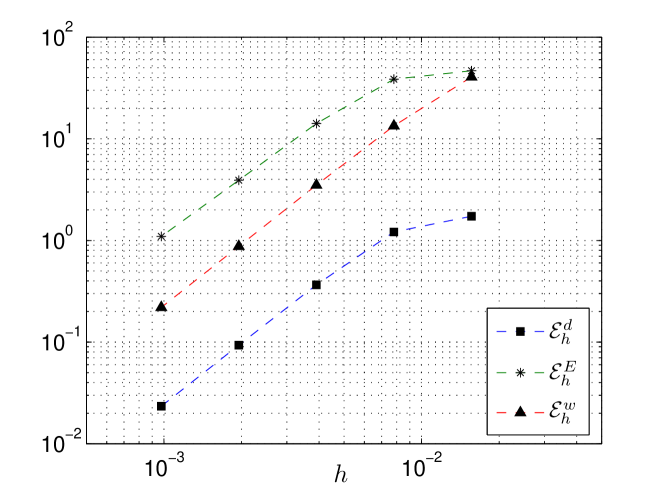
Figure 1. The errors $\mathcal{E}^{d}_{h}$, $\mathcal{E}^{w}_{h}$ and $\mathcal{E}^{E}_{h}$ for the approximations to (1.1) for a solution of the form (5.2) at time $T=20$ for $h=2^{-j}$, $j=6,\dots,10$.

In particular, (5.1) has solutions of the form

$$\begin{split}&\vartheta(t,x,y)\\ &\quad=\sum_{j=-J}^{J}\bigl{\{}a_{j}^{+}\sin(2\pi j(\sqrt{2}t+(x+y)))+a_{j}^{-}\sin(2\pi j(\sqrt{2}t-(x+y)))\\ &\quad\hphantom{=\sum_{j=-J}^{J}\bigl{\{}}+b_{j}^{+}\cos(2\pi j(\sqrt{2}t+(x+y)))+b_{j}^{-}\cos(2\pi j(\sqrt{2}t-(x+y)))\\ &\quad\hphantom{=\sum_{j=-J}^{J}\bigl{\{}}+c_{j}^{+}\sin(2\pi j(\sqrt{2}t+(x-y)))+c_{j}^{-}\sin(2\pi j(\sqrt{2}t-(x-y)))\\ &\quad\hphantom{=\sum_{j=-J}^{J}\bigl{\{}}+d_{j}^{+}\cos(2\pi j(\sqrt{2}t+(x-y)))+d_{j}^{-}\cos(2\pi j(\sqrt{2}t-(x-y)))\bigr{\}},\end{split}$$ (5.2)

for $J\geq 0$.

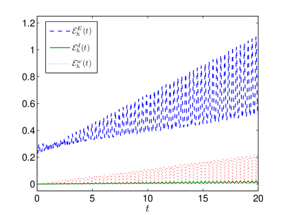
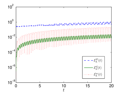
Figure 2. The evolution of the errors $\mathcal{E}^{d}_{h}(t)$, $\mathcal{E}^{w}_{h}(t)$ and $\mathcal{E}^{E}_{h}(t)$ versus time for the approximations to (1.1) for a solution of the form (5.2) for $h=2^{-10}$. Left: Real error, right: Error in log-scale.

In Figure 1, we have plotted the errors between the approximations $d_{h}$ and $d$, $w_{h}$ and $w$ respectively, in the $L^{2}$-norm and in the energy norm, that is

$$\mathcal{E}^{d}_{h} :=\sup_{m}\|d(t^{m},\cdot)-d^{m}_{h}\|_{L^{2}(\Omega)}$$

$$\mathcal{E}^{w}_{h} :=\sup_{m}\|w(t^{m},\cdot)-w^{m}_{h}\|_{L^{2}(\Omega)}$$

$$\mathcal{E}^{E}_{h} :=\sup_{m}\sqrt{\|\nabla d(t^{m},\cdot)-\nabla_{h}d^{m}_{h}\|_{L^{2}(\Omega)}^{2}+\|d_{t}(t^{m},\cdot)-D_{t}d^{m}_{h}\|_{L^{2}(\Omega)}^{2}}$$

for $a_{1}^{+}=a_{1}^{-}=1/4$, $a_{2}^{+}=a_{2}^{-}=1/10$, $b_{1}^{+}=-b_{1}^{-}=-2$, $b_{2}^{+}=-b_{2}^{-}=1/100$, $T=20$, $\Delta t=0.5h$, and $\Omega=\mathbb{T}^{2}$. Moreover, $h_{j}=2^{-j}$, $j=6,\dots,10$ for tolerance $\epsilon_{0}=h^{2}$. We observe a rate of convergence of almost $2$ for $\mathcal{E}^{d}_{h}$ and $\mathcal{E}^{w}_{h}$ and about $1.8$ for $\mathcal{E}^{E}_{h}$ (Table 1). Other choices of $\epsilon_{0}$ such as $h^{3/2}$ or $h^{3}$ gave similar results.

h	$\mathcal{E}_{h}^{d}$	$\mathcal{E}_{h}^{E}$	$\mathcal{E}_{h}^{w}$
$2^{-6}$	1.731	46.78	40.58
$2^{-7}$	1.213	38.64	13.42
$2^{-8}$	0.366	14.15	3.499
$2^{-9}$	0.093	3.915	0.877
$2^{-10}$	0.023	1.096	0.219
Rate	$1.56$	$1.35$	$1.88$

Table 1. Errors for different mesh resolutions for (1.1), (5.2) at time $T=20$, $\Delta t=0.5h$ and average rate for grid sizes $2^{-6}$ to $2^{-10}$.

In Figure 2, the evolution of the errors $\mathcal{E}^{\alpha}_{h}(t)$, $\alpha\in\{d,w,E\}$ , where $\mathcal{E}^{d}_{h}(t):=\|d(t,\cdot)-d_{h}(t,\cdot)\|_{L^{2}(\Omega)}$, and the other two defined in a similar way, for $h=2^{-10}$ versus time is shown. It appears that after an initial exponential increase, the error increases linearly with time.

5.2. Initial data developing singularities

In our second experiment, we compare the approximations computed by (2.1)–(2.2) to those obtained with the algorithms from [3].

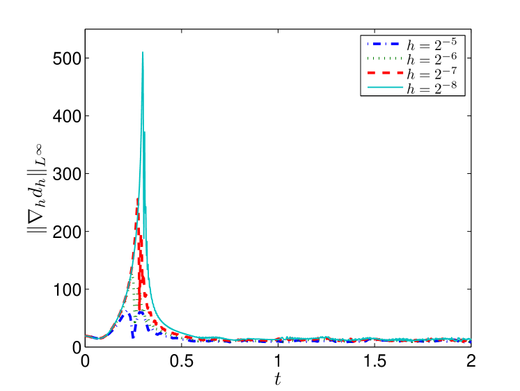
Figure 3. The evolution of $\|\nabla_{h}d_{h}\|_{L^{\infty}(\Omega)}$ versus time for initial data (5.3).

Specifically, we compute approximations for the initial data,

$$d^{0}(x,y)=\begin{cases}(0,0,-1)^{T},&r\geq 1/2,\\ (2xa,2ya,a^{2}-r^{2})^{T}/(a^{2}+r^{2}),&r<1/2,\end{cases},\quad w^{0}(x,y)\equiv 0,$$ (5.3)

on $D=[-0.5,0.5]^{2}$, where $r:=\sqrt{x^{2}+y^{2}}$ and $a(r)=(1-2r)^{4}$ up to time $T=2$, with CFL-condition $\Delta t=0.5h$, $h=2^{-j}$ for $j=5,6,7,8$ and tolerance $\epsilon_{0}=h^{2}$. As in [3], we observe a blow-up of the gradient $\nabla d$ in the $L^{\infty}$-norm around time $T=0.3$, cf. Figure 3.

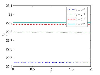
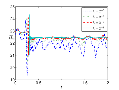
Figure 4. The evolution of $E_{m}$ and $H_{m}$ versus time for initial data (5.3).

The approximation ${E}_{m}^{\overline{s}}$ of the discrete energy (2.5) is close to being preserved, as we see in Figure 4, left hand side. In the same figure, on the right hand side, we have plotted the quantity

$$H_{m}:=\frac{1}{2}\int_{\Omega}|D_{t}d^{m}_{h}|^{2}+|\nabla_{h}d^{m}_{h}|^{2}\,dx,$$

which is not conserved by our scheme, but upper bounded. We observe some larger oscillations around the time of blow-up of $\nabla_{h}d_{h}$ in the $L^{\infty}$-norm.

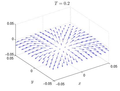
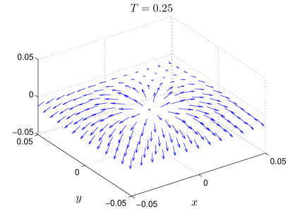
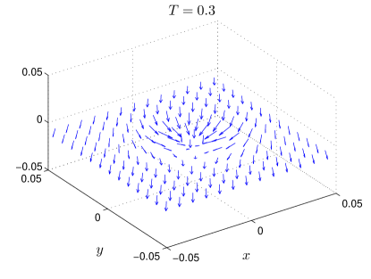
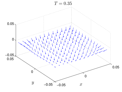
Figure 5. The approximation by (2.1)–(2.2) for initial data (5.3) in a neighborhood of the origin before and after blow-up time on a grid with $h=2^{-7}$.

In Figure 5 the approximation of (1.1), (5.3) in a neighborhood of the origin near blow-up time is shown. We observe that the third component of $d$ first switches sign away from the origin and then closer to it, which seems to cause the blow-up in the gradient of $d$.

References

- [1] L. Banas, A. Prohl, and R. Schatzle, Finite element approximations of harmonic map heat flows and wave maps into spheres of nonconstant radii, Numer. Math., 115, (2010), 395–432.
- [2] S. Bartels, C. Lubich, and A. Prohl, Convergent discretization of heat and wave map flows to spheres using approximate discrete Lagrange multipliers, Math. Comp, 78, (2009), 1269–1292.
- [3] S. Bartels, X. Feng, and A. Prohl, Finite element approximations of wave maps into spheres, SIAM J. Numer. Anal., 46(1), 2008, 61–87.
- [4] S. Bartels, Semi-Implicit Approximation of Wave Maps into Smooth or Convex Surfaces, SIAM J. Numer. Anal., 47(5), 2009, 3486–3506.
- [5] J. Shatah and M. Struwe, Geometric wave equations, Courant Lecture Notes in Mathematics, 2, 1998.