Two-dimensional nonlinear travelling waves
in magnetohydrodynamic channel flow

Abstract

This study is concerned with the stability of a flow of viscous conducting liquid driven by a pressure gradient in the channel between two parallel walls subject to a transverse magnetic field. Although the magnetic field has a strong stabilizing effect, this flow, similarly to its hydrodynamic counterpart – plane Poiseuille flow – is known to become turbulent significantly below the threshold predicted by linear stability theory. We investigate the effect of the magnetic field on two-dimensional nonlinear travelling-wave states which are found at substantially subcritical Reynolds numbers starting from $\textit{Re}{}_{n}=2939$ without the magnetic field and from $\textit{Re}{}_{n}\sim 6.50\times 10^{3}\textit{Ha}$ in a sufficiently strong magnetic field defined by the Hartmann number $\textit{Ha}.$ Although the latter value is by a factor of seven lower than the linear stability threshold $\textit{Re}{}_{l}\sim 4.83\times 10^{4}\textit{Ha},$ it is still more than an order of magnitude higher than the experimentally observed value for the onset of turbulence in the magnetohydrodynamic (MHD) channel flow.

1 Introduction

The flow of viscous incompressible liquid driven by a constant pressure gradient in the channel between two parallel walls, which is generally known as plane Poiseuille or simply channel flow, is one of the simplest and most extensively studied models of hydrodynamic instabilities and transition to turbulence in shear flows (Yaglom, 2012). The development of turbulence in the magnetohydrodynamic (MHD) counterpart of this flow, which is known as Hartmann flow and arises when a conducting liquid flows in the presence of a transverse magnetic field, is currently not so well understood. The MHD channel flow, which was first described theoretically by Hartmann (1937) and then studied experimentally by Hartmann & Lazarus (1937) is still an active subject of research (Hagan & Priede, 2013b; Krasnov et al., 2013).

Linear stability of Hartmann flow was first analysed by Lock (1955), who showed that the magnetic field has a strong stabilizing effect which results in the critical Reynolds number increasing from $\textit{Re}_{l}=5772.2$ without the magnetic field to $\textit{Re}_{l}\sim 50\,000\textit{Ha}$ for Hartmann numbers $\textit{Ha}\gtrsim 20.$ The critical Reynolds number for the linear stability threshold based on the Hartmann layer thickness $R_{l}=\textit{Re}_{l}/\textit{Ha}\approx 50\,000$ is more than two orders of magnitude higher than $R_{t}\approx 225$ at which transition from turbulent to laminar MHD channel flow was experimentally observed by Murgatroyd (1953). This extremely high critical Reynolds number found by Lock (1955), which is typical for exponential velocity profiles (Roberts, 1967; Drazin & Reid, 1981; Pothérat, 2007), has been confirmed by a number of more accurate subsequent studies starting with Likhachev (1976), who found $R_{l}\approx 48\,310,$ which is very close to the highly accurate $R_{l}\approx 48\,311.016$ obtained later by Takashima (1996). Linear stability analysis of a single Hartmann layer has been carried out by Lingwood & Alboussière (1999) using a relatively rough numerical approach which produced $R_{l}\approx 48\,250.$

The result of Murgatroyd (1953) was, in turn, confirmed by Brouillette & Lykoudis (1967) as well as by Branover (1967). A somewhat higher threshold value of $R_{t}\approx 380$ was found in the latest experiment on the transition to turbulence in the Hartmann layer by Moresco & Alboussière (2004). This value was supported by the accompanying numerical study of Krasnov et al. (2004), who reported $R_{t}$ in the range between $350$ and $400$ (for more detailed discussion of these results, see the recent review by Zikanov et al. 2014).

A possible cause of the discrepancy between the theory and experiment was suggested by Lock (1955) himself who conjectured that it may be due to the finite amplitude of the disturbance which is not taken into account by the linear stability analysis. This conjecture was supported by the weakly nonlinear stability analysis of a physically similar asymptotic suction boundary layer, which was found by Hocking (1975) and Likhachev (1976) to be subcritically unstable with respect to small but finite-amplitude disturbances. Moresco & Alboussière (2003) later confirmed the same to be the case also for the Hartmann layer also. The first quantitative results concerning finite-amplitude subcritical travelling waves in Hartmann flow were reported by Lifshits & Shtern (1980). Assuming the perturbation to be in the form of a single harmonic, which is known as the mean-field approximation, they found such two-dimensional (2D) travelling waves to exist down to the local Reynolds number $R_{n}=\textit{Re}_{n}/\textit{Ha}\approx 12\,300.$ The use of this approximation is endorsed by its unexpectedly good performance in the non-magnetic case, where it produces $\textit{Re}_{n}\approx 2825$ (Soibelman & Meiron, 1991), which differs by less than $4\%$ from the accurate result $\textit{Re}_{n}\approx 2939$ (Casas & Jorba, 2012). On the other hand, this approximation is known to be only qualitatively correct even in the weakly nonlinear limit where it overestimates the first Landau coefficient, which determines the evolution of small finite-amplitude disturbances, by about $30\%$ (Reynolds & Potter, 1967).

Alternatively, there have been attempts to explain the transition to turbulence in Hartmann flow by the energy stability and the transient growth theories. Although the former formally applies to arbitrary disturbance amplitudes, it is essentially a linear and amplitude-independent approach because the nonlinear term neither produces nor dissipates the energy and, thus, drops out of the disturbance energy balance. Using this approach Lingwood & Alboussière (1999) found that the Hartmann layer is energetically stable, i.e., all disturbances decay at any time, when the local Reynolds number is below $R_{e}\approx 26,$ which is almost an order of magnitude lower than the experimentally observed threshold. As demonstrated in the numerical study by Krasnov et al. (2004), also the optimal transient growth which has been studied for the Hartmann boundary layer by Gerard-Varet (2002) and for the whole Hartmann flow by Airiau & Castets (2004).

Transition to turbulence is essentially a nonlinear process which is mediated by the equilibrium states that may exist besides the laminar base flow at sufficiently high Reynolds numbers. However, though such equilibrium states are usually unstable, they may have stable manifolds that approach very close to the laminar base flow (Chapman, 2002). Thus, a small finite-amplitude perturbation can easily bring the flow into the stable manifold of such an equilibrium state. First, the initial perturbation is amplified as it is attracted to the equilibrium state along the stable manifold. Second, when the flow gets sufficiently close to the equilibrium state, it is repelled along the unstable manifold leading to another state. This may result in the flow wandering between a number of such unstable equilibrium states which form the so-called ‘skeleton of turbulence’. For the significance of such states in turbulent flows, see the review by Kawahara et al. (2012). It has to be noted that the existence of multiple equilibrium states is inherently a nonlinear effect which has little to do with the non-normality linear problem underlying the transient growth (Waleffe, 1995). Moreover, as the evolution of the flow is determined by its initial state, it is not the transient growth but rather the finite amplitude of the initial perturbation which is required for the flow to get into the basin of attraction of another equilibrium state. Even the so-called optimal perturbations formed by the streamwise rolls, which lie at the heart of the transient growth mechanism, require an additional finite-amplitude perturbation to reach turbulent attractor. The breakdown of the streamwise rolls cannot be explained by their apparent linear instability because because no infinitesimal disturbance can reach finite amplitude required for the transition to turbulence over the finite lifetime of these rolls. The gap between the linear transient growth and the nonlinear dynamical system approach is bridged by the optimisation approach recently reviewed by Kerswell et al. (2014).

The present study, constituting the first step of a fully nonlinear stability analysis, is concerned with finding 2D travelling-wave states in Hartmann flow. Starting from plane Poiseuille flow, we trace such subcritical equilibrium states by gradually increasing the magnetic field. Using an accurate numerical method based on the Chebyshev collocation approximation and a sufficiently large number of harmonics we find that such states extend to the local subcritical Reynolds number $R_{n}\approx 6500$ which is almost a factor of two smaller than that predicted by the mean-field approximation (Lifshits & Shtern, 1980).

The paper is organized as follows. The problem is formulated in $\S$2. In $\S$3 we present theoretical background concerning 2D nonlinear travelling-wave states. The Numerical method and the solution procedure are outlined in $\S$4. In $\S$5 we present and discuss numerical results concerning 2D nonlinear travelling waves and their linear stability with respect to 2D superharmonic disturbances. The paper is concluded with a summary in $\S$6.

2 Formulation of problem

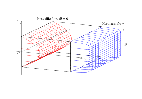
Figure 1: Sketch of the problem showing velocity profiles of Poiseuille and Hartmann flows.

Consider the flow of an incompressible viscous electrically conducting liquid with density $\rho,$ kinematic viscosity $\nu$ and electrical conductivity $\sigma$ driven by a constant gradient of pressure $p$ in a channel of width $2h$ between two parallel walls in the presence of a transverse homogeneous magnetic field $\boldsymbol{\mathit{B}}$. The velocity distribution of the flow $\boldsymbol{\mathit{v}}(\boldsymbol{\mathit{r}},t)$ is governed by the Navier-Stokes equation

$$\partial_{t}\boldsymbol{\mathit{v}}+(\boldsymbol{\mathit{v}}\cdot\boldsymbol{\mathit{\nabla}})\boldsymbol{\mathit{v}}=-\rho^{-1}\boldsymbol{\mathit{\nabla}}p+\nu\boldsymbol{\mathit{\nabla}}^{2}\boldsymbol{\mathit{v}}+\rho^{-1}\boldsymbol{\mathit{f}},$$ (1)

where $\boldsymbol{\mathit{f}}=\boldsymbol{\mathit{j}}\times\boldsymbol{\mathit{B}}$ is the electromagnetic body force containing the induced electric current $\boldsymbol{\mathit{j}},$ which is governed by Ohm’s law for a moving medium

$$\boldsymbol{\mathit{j}}=\sigma(\boldsymbol{\mathit{E}}+\boldsymbol{\mathit{v}}\times\boldsymbol{\mathit{B}}),$$ (2)

where $\boldsymbol{\mathit{E}}$ is the electric field in the stationary frame of reference. The flow is assumed to be sufficiently slow that the induced magnetic field is negligible relative to the imposed one. This supposes a small magnetic Reynolds number $\textit{Rm}=\mu_{0}\sigma v_{0}L\ll 1,$ where $\mu_{0}$ is the permeability of vacuum and $v_{0}$ and $L$ are the characteristic velocity and length scale of the flow, respectively. Using the thickness of the Hartmann layer $L=\delta=B^{-1}\sqrt{\rho\nu/\sigma}$ as the relevant length scale in strong magnetic field, we have $\textit{Rm}\sim R\textit{Pm},$ where $R=\textit{Re}/\textit{Ha}$ is a local Reynolds number based on $\delta$ and Pm is the magnetic Prandtl number. Taking into account that for typical liquid metals $\textit{Pm}\sim 10^{-5},$ the constraint on Rm translates into $R\ll\textit{Pm}^{-1}\sim 10^{5}.$ In addition, we assume that the characteristic time of velocity variation $\tau\sim L/v_{0}$ is much longer than the magnetic diffusion time $\tau_{m}=\mu_{0}\sigma L^{2}.$ This is also satisfied by the constraint on Rm and thus allows us to use the quasi-stationary approximation leading to $\boldsymbol{\mathit{E}}=-\boldsymbol{\mathit{\nabla}}\phi,$ where $\phi$ is the electrostatic potential (Roberts, 1967).

The velocity and current satisfy mass and charge conservation $\boldsymbol{\mathit{\nabla}}\cdot\boldsymbol{\mathit{v}}=\boldsymbol{\mathit{\nabla}}\cdot\boldsymbol{\mathit{j}}=0.$ Applying the latter to Ohm’s law (2) yields

$$\boldsymbol{\mathit{\nabla}}^{2}\phi=\boldsymbol{\mathit{B}}\cdot\boldsymbol{\mathit{\omega}},$$ (3)

where $\boldsymbol{\mathit{\omega}}=\boldsymbol{\mathit{\nabla}}\times\boldsymbol{\mathit{v}}$ is vorticity. At the channel walls $S$, the normal $(n)$ and tangential $(\tau)$ velocity components satisfy the impermeability and no-slip boundary conditions $\left.v_{n}\right|_{s}=0$ and $\left.v_{\tau}\right|_{s}=0.$

We employ right-handed Cartesian coordinates with the origin set at the mid-height of the channel, and the $x$- and the $z$-axes directed, respectively, against the applied pressure gradient $\boldsymbol{\mathit{\nabla}}p_{0}=P\boldsymbol{\mathit{e}}_{x}$ and along the magnetic field $\boldsymbol{\mathit{B}}=B\boldsymbol{\mathit{e}}_{z}$ so that the channel walls are located at $z=\pm h,$ as shown in figure 1, and the velocity is defined as $\boldsymbol{\mathit{v}}=(u,v,w).$ Subsequently, all variables are non-dimensionalized by using $h,$ $h^{2}/\nu$ and $Bh\nu$ as the length, time and electric potential scales, respectively. The velocity is scaled by the viscous diffusion speed $\nu/h,$ which we employ as the characteristic velocity instead of the commonly used centreline velocity.

The problem admits a rectilinear base flow

$$\boldsymbol{\mathit{v}}_{0}(z)=\bar{u}_{0}(z)\boldsymbol{\mathit{e}}_{x}=\textit{Re}\,\bar{u}(z)\boldsymbol{\mathit{e}}_{x}$$ (4)

for which (1) reduces to

$$\bar{u}^{\prime\prime}-\textit{Ha}^{2}\bar{u}=\bar{P},$$ (5)

where $\textit{Re}=Uh/\nu$ is the Reynolds number based on the centreline velocity $U$ of unperturbed flow, $\textit{Ha}=Bh\sqrt{\sigma/\rho\nu}$ is the Hartmann number, and $\bar{P}$ is a dimensionless coefficient which relates $U$ with the applied pressure gradient $P=\bar{P}U\nu\rho/h^{2}$ by satisfying the normalization condition $\bar{u}(0)=1.$ This Reynolds number is convenient for characterizing a flow driven by a fixed pressure gradient. Besides this so-called pressure Reynolds number, one can also use a Reynolds number based on the flow rate, $\textit{Re}_{q},$ which is more suitable for the case of fixed flow rate and will be introduced in $\S$5. Note that the use of either of these two Reynolds numbers is a matter of convenience as long as one remains a time-independent function of the other. Equation (5) defines the well-known Hartmann flow profile

$$\bar{u}(z)=\frac{\cosh(\textit{Ha})-\cosh(z\textit{Ha})}{\cosh(\textit{Ha})-1}$$ (6)

with $\bar{P}=-\frac{\textit{Ha}^{2}\cosh(\textit{Ha})}{\cosh(\textit{Ha})-1},$ which corresponds to a channel with perfectly conducting walls. In a weak magnetic field $(\textit{Ha}\ll 1),$ the Hartmann flow reduces to the classic plane Poiseuille flow $\bar{u}(z)=1-z^{2}.$

Note that electrical conductivity of the walls affects only the relationship between the applied pressure gradient and the centreline velocity but not the profile of the Hartmann flow. Thus, the stability of Hartmann flow with respect to transverse 2D disturbances, which are not affected by the conductivity of the walls, is determined entirely by the centreline velocity. This is the case considered in the present study.

3 Theoretical background

3.1 Linear stability of the base flow

The two-dimensional travelling waves considered in this study are expected to emerge as the result of linear instability of the Hartmann flow (4) with respect to infinitesimal perturbations $\boldsymbol{\mathit{v}}_{1}(\boldsymbol{\mathit{x}},t).$ Owing to the invariance of the base flow in both $t$ and $\boldsymbol{\mathit{x}}=(x,y),$ perturbations are sought as Fourier modes

$$\boldsymbol{\mathit{v}}_{1}(\boldsymbol{\mathit{r}},t)=\boldsymbol{\mathit{\hat{v}}}(z)\mathrm{e}^{\lambda t+\mathrm{i}\boldsymbol{\mathit{k}}\cdot\boldsymbol{\mathit{x}}}+\mbox{c.c.}$$ (7)

defined by the complex amplitude distribution $\boldsymbol{\mathit{\hat{v}}}(z)$, temporal growth rate $\lambda$ and the wave vector $\boldsymbol{\mathit{k}}=(\alpha,\beta).$ The incompressibility constraint, which takes the form $\boldsymbol{\mathit{D}}_{k}\cdot\boldsymbol{\mathit{\hat{v}}}=0,$ where $\boldsymbol{\mathit{D}}_{k}\equiv\boldsymbol{\mathit{e}}_{z}\frac{\mathrm{d}\,}{\mathrm{d}z}+\mathrm{i}\boldsymbol{\mathit{k}}$ is a spectral counterpart of the nabla operator, is satisfied by expressing the component of the velocity perturbation in the direction of the wave vector as $\hat{u}_{\shortparallel}=\boldsymbol{\mathit{e}}_{\shortparallel}\cdot\boldsymbol{\mathit{\hat{v}}}=\mathrm{i}k^{-1}\hat{w}^{\prime},$ where $\boldsymbol{\mathit{e}}_{\shortparallel}=\boldsymbol{\mathit{k}}/k$ and $k=|\boldsymbol{\mathit{k}}|.$ Taking the curl of the linearized counterpart of (1) to eliminate the pressure gradient and then projecting it onto $\boldsymbol{\mathit{e}}_{z}\times\boldsymbol{\mathit{e}}_{\shortparallel},$ after some transformations we obtain a modified Orr-Sommerfeld-type equation which includes a magnetic term

$$\lambda\boldsymbol{\mathit{D}}_{k}^{2}\hat{w}=\left[\boldsymbol{\mathit{D}}_{k}^{4}-\textit{Ha}^{2}(\boldsymbol{\mathit{e}}_{z}\cdot\boldsymbol{\mathit{D}}_{k})^{2}+\mathrm{i}k\textit{Re}(\bar{u}^{\prime\prime}-\bar{u}\boldsymbol{\mathit{D}}_{k}^{2})\right]\hat{w}.$$ (8)

The no-slip and impermeability boundary conditions require

$$\hat{w}=\hat{w}^{\prime}=0\quad\mbox{at}\quad z=\pm 1.$$ (9)

The equation above is written in a non-standard form corresponding to our choice of the characteristic velocity. Note that the Reynolds number appears in this equation as a factor in the convective term rather than its reciprocal in the viscous term as in the standard form. As a result, the growth rate $\lambda$ differs by a factor Re from its standard definition.

Since equation (8) like its non-magnetic counterpart admits Squire’s transformation, in the following we consider only two-dimensional perturbations $(k=\alpha),$ which are the most unstable (Lock, 1955). The problem is solved numerically using the Chebyshev collocation method which is described in detail by Hagan & Priede (2013a).

3.2 2D nonlinear travelling waves

Two-dimensional travelling waves emerge as follows. First, the neutrally stable mode (7) with a purely real frequency $\omega=-\mathrm{i}\lambda$ interacting with itself through the quadratically nonlinear term in (1) produces a steady streamwise-invariant perturbation of the mean flow as well as a second harmonic $\sim\mathrm{e}^{2\mathrm{i}(\omega t+\alpha x)}.$ Further nonlinear interactions produce higher harmonics, which similarly to the fundamental and second harmonic travel with the same phase speed $c=-\omega/\alpha.$ Thus, the solution can be sought in the form

$$\boldsymbol{\mathit{v}}(\boldsymbol{\mathit{r}},t)=\sum_{n=-\infty}^{\infty}E^{n}\boldsymbol{\mathit{\hat{v}}}_{n}(z),$$ (10)

where $E=\mathrm{e}^{\mathrm{i}(\omega t+\alpha x)}$ contains $\omega,$ which needs to determined together $\boldsymbol{\mathit{\hat{v}}}_{n}$ by solving a nonlinear eigenvalue problem (Huerre & Rossi, 1998). The reality of solution requires $\boldsymbol{\mathit{\hat{v}}}_{-n}=\boldsymbol{\mathit{\hat{v}}}_{n}^{*},$ where the asterisk stands for the complex conjugate. The incompressibility constraint applied to the $n$th velocity harmonic results in $\boldsymbol{\mathit{D}}_{\alpha_{n}}\cdot\boldsymbol{\mathit{\hat{v}}}_{n}=0,$ where $\boldsymbol{\mathit{D}}_{\alpha_{n}}\equiv\boldsymbol{\mathit{e}}_{z}\frac{\mathrm{d}\,}{\mathrm{d}z}+\mathrm{i}\boldsymbol{\mathit{e}}_{x}\alpha_{n}$ with $\alpha_{n}=\alpha n$ stands for the spectral counterpart of the nabla operator. This constraint can be satisfied by expressing the streamwise velocity component

$$\hat{u}_{n}=\boldsymbol{\mathit{e}}_{x}\cdot\boldsymbol{\mathit{\hat{v}}}_{n}=\mathrm{i}\alpha_{n}^{-1}\hat{w}_{n}^{\prime}$$ (11)

in terms of the transverse component $\hat{w}_{n}=\boldsymbol{\mathit{e}}_{z}\cdot\boldsymbol{\mathit{\hat{v}}}_{n},$ which we employ instead of the commonly used stream function. Henceforth, the prime is used as a shorthand for $d/dz.$ Note that (11) is not applicable to the zeroth harmonic, for which it yields $\hat{w}_{0}\equiv 0.$ Thus, $\hat{u}_{0}$ needs to be considered separately in this velocity-based formulation.

Taking the curl of (1) to eliminate the pressure gradient and then projecting it onto $\boldsymbol{\mathit{e}}_{y},$ we obtain

$$[\boldsymbol{\mathit{D}}_{\alpha_{n}}^{2}-\mathrm{i}\omega n]\hat{\zeta}_{n}-\textit{Ha}^{2}\hat{u}_{n}^{\prime}=\hat{h}_{n},$$ (12)

where

$$\hat{\zeta}_{n}=\boldsymbol{\mathit{e}}_{y}\cdot\boldsymbol{\mathit{D}}_{\alpha_{n}}\times\boldsymbol{\mathit{\hat{v}}}_{n}=\begin{cases}\mathrm{i}\alpha_{n}^{-1}\boldsymbol{\mathit{D}}_{\alpha_{n}}^{2}\hat{w}_{n},&n\not=0;\\ \hat{u}_{0}^{\prime},&n=0.\end{cases}$$ (13)

and

$$\hat{h}_{n}={\displaystyle\sum_{m}}\boldsymbol{\mathit{\hat{v}}}_{n-m}\cdot\boldsymbol{\mathit{D}}_{\alpha_{m}}\hat{\zeta}_{m}$$ (14)

are the $y$-components of the $n$th harmonic of the vorticity $\boldsymbol{\mathit{\zeta}}=\boldsymbol{\mathit{\nabla}}\times\boldsymbol{\mathit{v}}$ and that of the curl of the nonlinear term $\boldsymbol{\mathit{h}}=\boldsymbol{\mathit{\nabla}}\times(\boldsymbol{\mathit{v}}\cdot\boldsymbol{\mathit{\nabla}})\boldsymbol{\mathit{v}}.$ Henceforth, the omitted summation limits are assumed to be infinite. Separating the terms involving $\hat{u}_{0}$ in (14), it can be rewritten as $\hat{h}_{n}=\mathrm{i}\alpha_{n}^{-1}(\hat{h}_{n}^{w}+\hat{h}_{n}^{u}),$ where

$$\hat{h}_{n}^{w} = n{\displaystyle\sum_{m\not=0}m^{-1}(}\hat{w}_{n-m}\boldsymbol{\mathit{D}}_{\alpha_{m}}^{2}\hat{w}_{m}^{\prime}-\hat{w}_{m}^{\prime}\boldsymbol{\mathit{D}}_{\alpha_{n-m}}^{2}\hat{w}_{n-m}),$$ (15)

$$\hat{h}_{n}^{u} = \mathrm{i}\alpha_{n}[\hat{u}_{0}-\hat{u}_{0}^{\prime\prime}\boldsymbol{\mathit{D}}_{\alpha_{n}}^{2}]\hat{w}_{n}\equiv\mathcal{N}_{n}(\hat{u}_{0})\hat{w}_{n}.$$ (16)

Eventually, using the expressions above, (12) can be written as

$$\mathcal{L}_{n}(\mathrm{i}\omega,\hat{u}_{0})\hat{w}_{n}=\hat{h}_{n}^{w},$$ (17)

with the operator

$$\mathcal{L}_{n}(\mathrm{i}\omega,\hat{u}_{0})=[\boldsymbol{\mathit{D}}_{\alpha_{n}}^{2}-\mathrm{i}\omega n]\boldsymbol{\mathit{D}}_{\alpha_{n}}^{2}-\textit{Ha}^{2}(\boldsymbol{\mathit{e}}_{z}\cdot\boldsymbol{\mathit{D}}_{\alpha_{n}})^{2}-\mathcal{N}_{n}(\hat{u}_{0}).$$ (18)

This equation governs all harmonics except the zeroth one, for which, in accordance with the incompressibility constraint (11), it implies $\hat{w}_{0}\equiv 0$. The zeroth velocity harmonic, which has only the streamwise component $\hat{u}_{0},$ is governed directly by the $x$-component of the Navier–Stokes equation (1):

$$\hat{u}_{0}^{\prime\prime}-\textit{Ha}^{2}\hat{u}_{0}=\hat{P}_{0}+\hat{g}_{0},$$ (19)

where $\hat{P}_{0}=\bar{P}\textit{Re}$ is a dimensionless mean pressure gradient and

$$\hat{g}_{0}=\mathrm{i}\sum_{m\not=0}\alpha_{m}^{-1}(\hat{w}_{m}^{*}\hat{w}_{m}^{\prime})^{\prime}$$ (20)

is the $x$-component of the zeroth harmonic of the nonlinear term $\boldsymbol{\mathit{g}}=(\boldsymbol{\mathit{v}}\cdot\boldsymbol{\mathit{\nabla}})\boldsymbol{\mathit{v}}.$ Velocity harmonics are subject to the usual no-slip and impermeability boundary conditions

$$\hat{w}_{n}=\hat{w}_{n}^{\prime}=\hat{u}_{0}=0\textrm{ at }z=\pm 1.$$ (21)

3.3 Linear stability of 2D travelling waves

Weakly subcritical equilibrium states, which exist in this case (Hagan & Priede, 2013b), are unconditionally unstable (Schmid & Henningson, 2001). This is because the growth rate of subcritical disturbances increases with their amplitude (Hagan & Priede, 2013b). Thus, a disturbance with an amplitude slightly lower or higher than the equilibrium one will respectively decay or grow so diverging from the equilibrium state. The stability of strongly subcritical equilibrium states is not obvious. Orszag & Patera (1983) originally suggested that the subcritical equilibrium state appearing at the linear stability threshold remains linearly unstable down the lowest possible Reynolds number admitting such states. At this limiting Reynolds number, which is the main concern of the present study, the unstable subcritical state disappears by merging with another equilibrium state of a higher amplitude. The latter was thought by Orszag & Patera (1983) to be linearly stable as in the saddle–node bifurcation. This simple picture was amended by Pugh & Saffman (1988) who showed that this is the case when the flow is driven by a fixed flow rate but not by a fixed pressure gradient. Although travelling-wave states at fixed flow rate are physically equivalent to those at fixed pressure gradient (Soibelman & Meiron, 1991), it is not the case in general when the flow rate and the mean pressure gradient depend not only on each other but also on time. First of all, the distinction between flows driven by fixed pressure gradient and fixed flow rate becomes important when the stability of travelling-wave states is considered.

Linear stability of the travelling-wave states, which in contrast to the rectilinear base state are periodic rather than invariant in both the time and the streamwise direction, is described by Floquet theory (Bender & Orsag, 1978; Herbert, 1988) according to which a small-amplitude velocity disturbance can be sought similarly to (10) as

$$\boldsymbol{\mathit{v}}_{1}(\boldsymbol{\mathit{r}},t)=e^{\tilde{\lambda}t}\sum_{n=-\infty}^{\infty}E^{n+\epsilon}\boldsymbol{\mathit{\tilde{v}}}_{n}(z)+\mbox{c.c.},$$ (22)

where $\tilde{\lambda}$ is generally a complex growth rate and $\epsilon$ is a real detuning parameter which defines the sideband wavenumber $\tilde{\alpha}=\epsilon\alpha$ (Huerre & Rossi, 1998), also called the subharmonic wavenumber by Soibelman & Meiron (1991). The case $\epsilon=0$ corresponds to the fundamental mode, which is also called superharmonic (Pugh & Saffman, 1988; Soibelman & Meiron, 1991), whereas $\epsilon=\pm\frac{1}{2}$ correspond to the so-called subharmonic mode. The disturbances with other values of $\epsilon$ are referred to as combination or detuned modes. Note that (22) with $\epsilon\pm 1$ is equivalent to the mode with $\epsilon$ and the index $n$ shifted by one. In addition, as seen from (22) the modes with $\pm\epsilon$ are complex conjugate. Thus, it suffices to consider $0\leq\epsilon<1$ or any other interval of $\epsilon$ of length one. Separating the two modes with opposite $z$-symmetries, as discussed in the next section, this interval can be reduced by half.

Adding disturbance (22) to the travelling-wave base state (10), we obtain a linearized counterpart of (12) for the transverse velocity harmonic $\tilde{w}_{n}:$

$$\left[\boldsymbol{\mathit{D}}_{\tilde{\alpha}_{n}}^{2}-\tilde{\lambda}-\mathrm{i}\omega n\right]\boldsymbol{\mathit{D}}_{\tilde{\alpha}_{n}}^{2}\tilde{w}_{n}-\textit{Ha}^{2}\tilde{w}_{n}^{\prime\prime}=-\mathrm{i}\tilde{\alpha}_{n}\sum_{m}\boldsymbol{\mathit{D}}_{\tilde{\alpha}_{n}}\cdot(\boldsymbol{\mathit{\hat{v}}}_{n-m}\tilde{\zeta}_{m}+\boldsymbol{\mathit{\tilde{v}}}_{m}\hat{\zeta}{}_{n-m}),$$ (23)

where $\tilde{\alpha}_{n}=\alpha_{n}+\tilde{\alpha}=(n+\epsilon)\alpha$ is a detuned wavenumber for the $n$th harmonic, $\tilde{u}_{n}=\boldsymbol{\mathit{e}}_{x}\cdot\boldsymbol{\mathit{\tilde{v}}}_{n}=\mathrm{i}\tilde{\alpha}_{n}^{-1}\tilde{w}_{n}^{\prime}$ is the streamwise velocity and $\tilde{\zeta}_{n}=\mathrm{i}\tilde{\alpha}_{n}^{-1}\boldsymbol{\mathit{D}}_{\tilde{\alpha}_{n}}^{2}\tilde{w}_{n}$ is the spanwise vorticity of the disturbance. The boundary conditions, as usual, are $\tilde{w}_{n}(1)=\tilde{w}_{n}^{\prime}(1)=0.$

Cutting the series (22) off at $n=\pm N,$ we obtain a linear eigenvalue problem represented by $2N+1$ complex equations (23) for the eigenvector consisting of the same number of harmonics $\tilde{w}_{n}$ with the eigenvalue $\tilde{\lambda},$ which depends on the subharmonic wavenumber $\tilde{\alpha}.$ This eigenvalue problem is solved in the same way as that for the linear stability of the rectilinear base flow. To avoid the division by zero in the expressions for $\tilde{u}_{0}$ and $\tilde{\zeta}_{0}$ above, which occurs for $\tilde{\alpha}=0,$ we use the substitution $\tilde{w}_{n}=-\mathrm{i}\tilde{\alpha}_{n}\tilde{\psi}_{n},$ where $\tilde{\psi}_{n}$ is the stream function. This makes superharmonic disturbances treatable in the same way as detuned ones. For the superharmonic disturbances corresponding to $\tilde{\alpha}\rightarrow 0,$ the eigenvalue problem becomes self-adjoint with $\tilde{w}_{-n}=\tilde{w}_{n}^{*},$ which means that eigenvalues are either real or complex conjugate.

Note that the detuned disturbances with $\tilde{\alpha}\not=0$ affect neither the mean pressure gradient nor the flow rate. Both of these quantities are associated with a zero-wavenumber mode, which occurs only for the fundamental disturbances $\epsilon=0$ when the zeroth harmonic of the streamwise velocity perturbation is an odd function of $z,$ i.e., $\tilde{u}_{0}(-z)=-\tilde{u}_{0}(z).$ This is the case for the fundamental modes with $z$-parities opposite to those of the travelling-wave state which are discussed in the next section.

The problem posed by (23) corresponds to the case of fixed flow rate. For $\tilde{\alpha}_{0}=0$ we have $\boldsymbol{\mathit{D}}_{\tilde{\alpha}_{0}}\equiv\boldsymbol{\mathit{e}}_{z}\frac{d\,}{dz}$ and thus for $n=0$ equation (23) can be integrated once. This results in a linearized counterpart of (19) for $\tilde{\psi}^{\prime}_{0}=\tilde{u}_{0}$ containing a constant of integration $\tilde{P}_{0}$ which represents perturbation of the mean pressure gradient:

$$\tilde{u}_{0}^{\prime\prime}-(\tilde{\lambda}+\textit{Ha}^{2})\tilde{u}_{0}=\sum_{m}(\hat{w}_{m}^{*}\tilde{u}_{m}+\hat{u}{}_{m}^{*}\tilde{w}_{m})^{\prime}+\tilde{P}_{0}.$$ (24)

Using this equation with $\tilde{P}_{0}=0$ instead of the original one we obtain a linear stability problem for the travelling waves driven by a fixed mean pressure gradient. Equation (24) can integrated once more leading to an equivalent equation in terms of $\tilde{\psi}{}_{0}$ which can be used instead (24). Alternatively, the integrated equation can be used as an effective but rather complicated boundary condition replacing the fixed flow rate condition $\tilde{\psi}_{0}(1)=0$ in the original equation (23) for $\tilde{\psi}_{0}$ (Soibelman & Meiron, 1991).

4 Numerical method

The problem is solved numerically using a Chebyshev collocation method with the Chebyshev-Lobatto nodes

$$z_{i}=\cos\left(i\pi/2M\right),\quad i=0,\cdots,M,$$ (25)

at which the discretized solution $(\hat{w}_{n},\hat{u}_{0})(z_{i})=(\tilde{w}_{n},\tilde{u}_{0})_{i}$ is sought in the upper half of the channel. The reduction to half the channel is due to the following symmetries implied by (15), which is the nonlinear term of the vorticity equation (12). The $z$-symmetry of this term is the same of as that of $\hat{w}_{n}$ governed by (12), and it is determined by the first derivative of the terms quadratic in $\hat{w}_{n}.$ Note that the first derivative inverts $z$-symmetry and the second derivative conserves it. Since the product of two harmonics with indices $m$ and $n$ produces two harmonics with the same $z$-symmetry and indices $n\pm m,$ which are separated by an even number $2m$, all harmonics with the same parity of indices have the same $z$-symmetry. Harmonics with even indices are produced by the products of harmonics with indices of the same parity, which have the same $z$-symmetry. Thus, these products are always even functions of $z.$ The inversion of the $z$-symmetry by the first derivative in the nonlinear term results in $\hat{w}_{n}$ with even $n$ being an odd function of $z.$ All harmonics with odd indices can have either odd or even $z$-symmetry depending on the symmetry of the fundamental mode $(n=1),$ which is usually determined by the linear stability analysis. This gives rise to two types of possible 2D solutions satisfying $\hat{w}_{n}(-z)=(-1)^{n+1}\hat{w}_{n}(z)$ and $\hat{w}_{n}(-z)=-\hat{w}_{n}(z)$, which are referred to as even or odd depending on the $z$-symmetry of the transverse velocity harmonics with odd indices. In secondary stability analysis, small-amplitude perturbations of each of these two solution branches splits into two further symmetry types. The first type of possible perturbation consists of the harmonics with the same $z$-parities as the travelling-wave solution itself, i.e. $\tilde{w}_{n}(-z)=(-1)^{n+1}\tilde{w}_{n}(z)$ and $\tilde{w}_{n}(-z)=-\tilde{w}_{n}(z)$ for even and odd branches, respectively. The second type of perturbations admitted by (23) consists of harmonics with $z$-symmetries opposite to those of the travelling-wave solution, i.e. $\tilde{w}_{n}(-z)=(-1)^{n}\tilde{w}_{n}(z)$ and $\tilde{w}_{n}(-z)=\tilde{w}_{n}(z)$ for even and odd branches, respectively (Pugh & Saffman, 1988). Note that for the even 2D solution branch, which consists of harmonics with alternating $z$-parities, one type of perturbation is changed into the other by the transformation $\epsilon\rightarrow\epsilon\pm 1$ which effectively shifts the index of harmonics in (22) by one.

Equations are approximated at the internal collocation points $1\leq i\leq M$ by using differentiation matrices which express the derivatives in terms of the collocation variables $(\boldsymbol{\mathsf{w}}_{n},\boldsymbol{\mathsf{u}}_{0})_{i}.$ Odd or even $z$-symmetry of each particular harmonic is taken into account by the reduced-size differentiation matrices based on the collocation points only in one half of the channel. The boundary conditions (9) are imposed at the boundary point $i=0$ (Peyret, 2002). When series (10) are truncated at $n=\pm N,$ (17) reduce to $N\times M$ complex algebraic equations with respect to the same number of complex unknowns $\boldsymbol{\mathsf{w}}_{n}$ for $n=1,2,\ldots,N.$ Note that $\boldsymbol{\mathsf{w}}_{0}\equiv 0$ and $\boldsymbol{\mathsf{w}}_{-n}=\boldsymbol{\mathsf{w}}_{n}^{*}.$ The equations also contain $M$ real unknowns $\tilde{u}_{0},$ which are governed by the same number of real equations resulting from the collocation approximation of (19). The equations are linear and, thus, directly solvable for $\tilde{u}_{0}$ in terms of $\boldsymbol{\mathsf{w}}_{n}$ by inverting the respective matrices. This leads to a system of $N\times M$ nonlinear complex equations for the same number of complex unknowns $\boldsymbol{\mathsf{w}}_{n}.$ Since the equations also contain $\boldsymbol{\mathsf{w}}_{n}^{*},$ the actual unknowns are the real and imaginary parts of $\boldsymbol{\mathsf{w}}_{n},$ which need to be determined by solving the same number, i.e. $2N\times M,$ of real equations represented by the real and imaginary parts of the original complex equations.

However, there is one more unknown: the frequency $\omega,$ which is the eigenvalue of this nonlinear problem, and needs to be determined along with $\boldsymbol{\mathsf{w}}_{n}.$ There are two ways to balance the number of unknowns and equations. First, as the problem is homogeneous, non-trivial solution requires a solvability condition to be satisfied, which provides another equation analogous to the characteristic determinant in the case of a linear eigenvalue problem. The second possibility, which is used here, follows from the fact that owing to the translational invariance of the problem $\boldsymbol{\mathsf{w}}_{n}$ is defined up an arbitrary phase. The phase, which determines the $x$-offset of the wave, can be fixed by imposing the condition $\Im[\boldsymbol{\mathsf{w}}_{1,i}]=0$ at some collocation point $i$ where the solution is not already fixed by boundary or symmetry conditions. This is equivalent to setting $\boldsymbol{\mathsf{w}}_{1,i}=A,$ where $A$ is a real parameter defining the amplitude of the transverse velocity. Thus, the number of unknowns is reduced by one and the system of $2N\times M$ nonlinear algebraic equations can be written in the general form

$$\boldsymbol{\mathsf{F}}(\boldsymbol{\mathsf{w}},A,\omega;\alpha,\textit{Re})\boldsymbol{\mathsf{w}}=\boldsymbol{\mathsf{0}},$$ (26)

where $\boldsymbol{\mathsf{w}}$ are the real and imaginary parts of $\boldsymbol{\mathsf{w}}_{n}$ normalized with the real amplitude $A$ and $\boldsymbol{\mathsf{F}}$ is a real square matrix of size $2N\times M$ depending on the listed parameters. For given $\alpha$ and $\textit{Re},$ this problem can be solved by the Newton-Raphson method with respect to $A,$ $\omega$ and $2N\times M-2$ unknown $\boldsymbol{\mathsf{w}}.$ In some cases, instead of $\textit{Re},$ it is more convenient to fix $A$ and then to solve for Re depending on $A$ and $\alpha.$

The solution is traced using a quadratic extrapolation along the arclength in logarithmic coordinates. For a general function $f(p)$ of an argument $p$ the scale-independent arclength element is defined as $\delta s^{2}=\ln^{2}(1+\frac{\delta f}{f})+\ln^{2}(1+\frac{\delta p}{p}).$ Starting with a reference arclength based on the solution at the first three chosen parameter values, a subsequent parameter value and an initial guess for the Newton-Raphson method are extrapolated from the previous three values. When Newton-Raphson iterations fail, the step size along the arclength is reduced until a solution is recovered, and then gradually increased to its original value as the solution is successfully traced.

5 Results

5.1 Nonlinear 2D travelling waves

$M\times N$	$\textit{Re}_{n}$	$\alpha_{n}$	$c_{n}=-\omega/\textit{Re}_{n}\alpha$	$A_{E}^{2}(\times 10^{3})$	$A=\hat{w}_{1}(0)$
$32\times 1$	$2825.56$	$1.22223$	$0.345828$	$6.14777$	$131.655$
$32\times 2$	$2701.72$	$1.31294$	$0.366290$	$4.92982$	$118.206$
$32\times 3$	$2911.36$	$1.31824$	$0.364025$	$4.33693$	$119.120$
$32\times 4$	$2933.53$	$1.32425$	$0.364470$	$4.50019$	$121.571$
$32\times 6$	$2940.08$	$1.31701$	$0.363147$	$4.26584$	$119.171$
$32\times 8$	$2939.05$	$1.31752$	$0.363251$	$4.28277$	$119.330$
$32\times 10$	$2939.04$	$1.31751$	$0.363250$	$4.28224$	$119.324$
$40\times 10$	$2939.04$	$1.31750$	$0.363249$	$4.28224$	$119.320$

Table 1: Critical parameters for the appearance of 2D travelling waves in plane Poiseuille flow computed with various number of collocation points $M$ and harmonics $N.$

Weakly nonlinear analysis shows that the instability of the Hartmann flow is invariably subcritical regardless of the magnetic field strength (Hagan & Priede, 2013b). In the present study, we determine how far the subcritical equilibrium states, which bifurcate from the Hartmann flow, extend below the linear stability threshold. Let us first validate our method described in Sec. 3.2 by computing the critical Reynolds number for 2D travelling waves in plane Poiseuille flow, which corresponds to $\textit{Ha}=0.$ By solving (26) for Re as a function of $A$ and $\alpha$ and then minimizing the solution over both variables we obtain the critical values which are shown in table 1 for various numbers of collocation points $M$ and harmonics $N.$ The critical parameters for the first three numerical resolutions perfectly agree with those found by Soibelman & Meiron (1991), whereas for the last three resolutions both Re and $\alpha$ agree up to 5 decimal points with the accurate results obtained by Casas & Jorba (2012) using $2M=70$ Chebyshev polynomials and $N=22$ Fourier modes. To characterize the deviation of the velocity distribution (10) from the base state (4), besides the transverse velocity amplitude $A$ introduced in (26), we also use the amplitude associated with the energy of perturbation scaled by the energy of the basic flow:

$$A_{E}^{2}=\int_{0}^{1}\left\langle|\boldsymbol{\mathit{v}}(x,z)-\boldsymbol{\mathit{v}}_{0}(z)|^{2}\right\rangle dz/\int_{0}^{1}|\boldsymbol{\mathit{v}}_{0}(z)|^{2}dz,$$ (27)

where the angle brackets stand for the streamwise average. This quantity slightly differs from that used by Soibelman & Meiron (1991) who neglect the contribution of the mean flow perturbation.

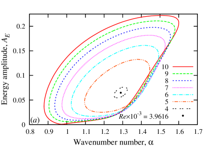
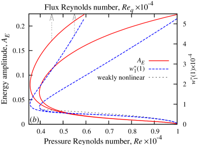
Figure 2: The energy amplitude of equilibrium states of the even mode versus the wavenumber $\alpha$ at various Re (a) and the extrema of the energy amplitude versus pressure Reynolds number Re (bottom axis) and versus the flux Reynolds number (top axis) (b) for $\textit{Ha}=1$ computed with the resolution $M\times N=32\times 8.$

We start with a relatively low Hartmann number $\textit{Ha}=1$ for which the flow becomes linearly unstable at $\textit{Re}_{l}=10016.3$ with respect to a mode with $\alpha_{l}=0.971827$ and even $z$-symmetry as in the non-magnetic case. The energy amplitude of equilibrium states versus the wavenumber is plotted in figure 2(a) for various subcritical values of $\textit{Re}.$ As for the non-magnetic plane Poiseuille flow, equilibrium states form closed contours, which shrink as Re is reduced, and collapse to a point at the critical $\textit{Re}_{n}=3961.36$ below which 2D travelling waves vanish. It means that subcritical perturbations have both a lower and an upper equilibrium amplitude. Both these amplitudes are plotted in figure 2(b) together with the respective value of $\hat{w}_{1}^{\prime\prime}(1),$ which is the quantity predicted by the weakly nonlinear analysis (Hagan & Priede, 2013b), versus the usual pressure Reynolds number on the bottom axis and versus the flux Reynolds number $\textit{Re}_{q}$ on the top axis. The latter is related to the original Reynolds number Re based on the mean pressure gradient:

$$\textit{Re}_{q}=\textit{Re}+\hat{\psi}_{0}(1)/\bar{\psi}(1),$$ (28)

where $\bar{\psi}(1)=\int_{0}^{1}\bar{u}(z)\,dz=(\cosh(\textit{Ha})-\textit{Ha}^{-1}\sinh(\textit{Ha}))/(\cosh(\textit{Ha})-1)$ is half of the flux carried by unperturbed Hartmann flow (6) and $\hat{\psi}_{0}(1)$ is the flow rate perturbation defined by (32) and plotted in figure 6(b) below. As seen, the lower branch of $\hat{w}_{1}^{\prime\prime}(1)$ is predicted well by the weakly nonlinear solution for subcritical Reynolds numbers down to $\textit{Re}\approx 7000.$

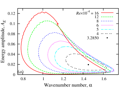
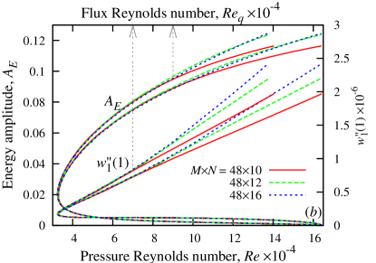
Figure 3: The energy amplitude of equilibrium states of the even mode versus the wavenumber $\alpha$ at various Re (a) and the extrema of the energy amplitude versus Re (b) for $\textit{Ha}=5$ computed with the resolutions $M\times N=48\times 16\cdots 32.$

A similar structure of subcritical equilibrium states is also seen in figure 3 for $\textit{Ha}=5$ when the flow becomes linearly unstable at $\textit{Re}_{l}=164\thinspace 154$ with respect to a perturbation of even $z$-symmetry. At this large Re it becomes difficult to compute accurately the upper equilibrium states which remain wiggly up to the numerical resolution of $48\times 32.$ Strongly subcritical states, which in this case extend down to $\textit{Re}_{n}\approx 32\thinspace 860,$ can reliably be computed with a substantially lower resolution of $48\times 16.$ This structure of the equilibrium states of the even mode is typical in the vicinity of the critical Reynolds number at higher Hartmann numbers also. In the following, we focus on such strongly subcritical Reynolds numbers at which 2D travelling waves emerge. The respective Reynolds number defines the 2D nonlinear stability threshold.

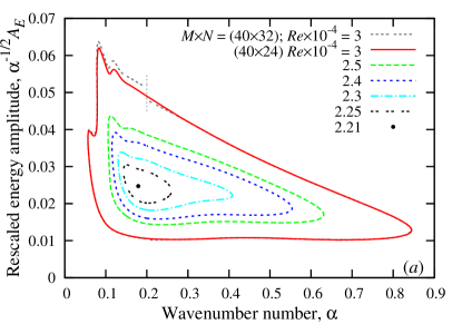
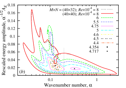
Figure 4: The energy amplitude of equilibrium states of the odd mode rescaled with $\alpha^{-1/2}$ versus the wavenumber $\alpha$ for $\textit{Ha}=5$ (a), $\textit{Ha}=10$ (b) and various Re close to the turning point. The wavenumbers $\alpha<0.2$ for $Re=3\times 10^{4},$ $N=32$ (a) and $Re=8\times 10^{4},$ $N=40$ (b) is rescaled, respectively with factors $32/24$ and $40/32.$

In contrast to Poiseuille flow, which can be linearly unstable only to perturbations of even $z$-symmetry, Hartmann flow can be linearly unstable also to perturbations of odd $z$-symmetry when $Ha\gtrsim 6.5$ (Hagan & Priede, 2013b). Subcritical equilibrium states of the odd mode, whose energy amplitudes are shown in figure 4 versus the wavenumber for $\textit{Ha}=5$ and $\textit{Ha}=10$ at several Reynolds numbers in the vicinity of the critical point, have a significantly different structure. Besides multiple minima and loopy structures, which are seen to form at $\textit{Ha}=10$ in figure 4(b), the main difference from the even mode is the extension of these states towards small wavenumbers. These apparently long-wave states have several numerical peculiarities. First, when the number of harmonics $N$ is increased, the wavelength of these states increases whereas their amplitude decreases. At the same time, the states with sufficiently short wavelength $(\alpha\gtrsim 0.2)$ converge. Although long-wave states do not appear to converge, the pattern of their equilibrium energy amplitude becomes self-similar at sufficiently large $N.$ Both the wavenumber $\alpha$ and the energy (27) for these states decrease inversely with $N.$ This is seen in figure 4(a) where the rescaled energy amplitude $\alpha^{-1/2}A_{E}$ computed for $Re=3\times 10^{4}$ with $N=32$ harmonics overlaps with the respective amplitude computed with $N=24$ harmonics when the range of wavenumbers $\alpha<0.2$ is rescaled with a factor of $\frac{32}{24}$. Note that the same results overlap without rescaling at larger $\alpha.$ Similar behaviour can be seen also in figure 4(b) where a much more complicated equilibrium amplitude distribution for $Re=8\times 10^{4}$ computed with $N=32$ closely overlaps with the respective distribution computed with $N=40$ when $\alpha<0.2$ is rescaled with a factor of $\frac{40}{32}.$ This rescaling has two implications. First, the relevant parameter for these apparently long-wave equilibrium states is not the wavenumber of the first harmonic $\alpha$ but that of the last harmonic given by$\alpha N.$ Second, these states are characterized by the integral perturbation energy over the wavelength $\propto\alpha^{-1}A_{E}^{2}$ rather by its streamwise average (27). These peculiar properties of the long-wave equilibrium states are due their unusual spatial structure which is revealed by the streamlines of the critical perturbation shown for $Ha=10$ in figure 7(b) below. Namely, these states turn out be localized rather than wave-like. Periodicity of these states is enforced by the Fourier series representation (10). The apparent period is determined by the fundamental wavenumber $\alpha$ which decreases inversely with the number of harmonics. At the same time, the actual solution contained in the higher harmonics converges to a definite integral energy as discussed above.

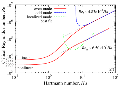
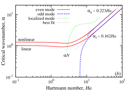
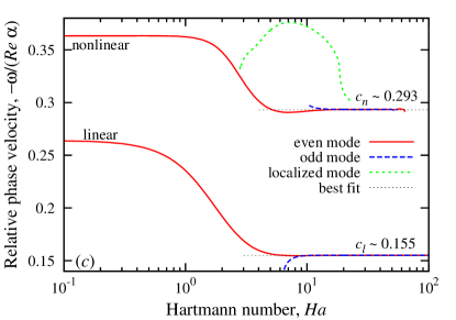
Figure 5: Critical Reynolds number (a), wavenumber (b) and phase speed (c) for even and odd modes of linear and nonlinear instabilities against the Hartmann number. The effective wavenumber of the localized (nonlinear odd) mode shown in figure 7(b) is given by $\alpha N,$ where $N$ is the number harmonics.

The critical Reynolds number and wavenumber for the 2D nonlinear stability threshold are shown in figure 5 together with critical parameters for linear stability versus the Hartmann number (Hagan & Priede, 2013b). At small Hartmann numbers, instability is associated with the even mode for which 2D travelling waves appear at $\textit{Re}_{n}=2939.$ This is the 2D nonlinear stability threshold of plane Poiseuille flow shown in table 1. When the Hartmann number exceeds $\textit{Ha}\approx 2.8,$ which is about half of the respective value for the linear instability, an odd equilibrium mode appears with a large Reynolds number and a small wavenumber. This long-wave odd mode exists only within a limited range of Hartmann numbers up to $\textit{Ha}\approx 20.$ At $\textit{Ha}\approx 10$ another odd mode appears with a slightly higher Reynolds number but much shorter wavelength. At $\textit{Ha}\approx 15$ the Reynolds number of the latter mode becomes smaller than that for the long-wave mode. The characteristics of this short-wave odd mode are seen to be closely approaching those of the original even mode. In a sufficiently strong magnetic field, the critical Reynolds number and wavenumber for both nonlinear modes increase with the Hartmann number similarly to the respective threshold parameters of the linear instability (Hagan & Priede, 2013b). Namely, for $\textit{Ha}\gtrsim 20$ the best fit yields

$$\textit{Re}_{n} \sim 6.50\times 10^{3}\textit{Ha},$$ (29)

$$\alpha_{n} \sim 0.223\textit{Ha},$$ (30)

$$c_{n} \sim 0.293.$$ (31)

It is important to notice that the critical Reynolds number above is almost an order of magnitude lower than that for the linear instability $\textit{Re}{}_{l}\sim 48\,300\textit{Ha}.$ In the mean-field approximation using only one harmonic, we find $\textit{Re}_{n}\sim 12\,300\textit{Ha},$ which is almost a factor of two higher than the accurate result above and coincides with the result reported by Lifshits & Shtern (1980).

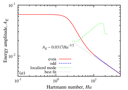
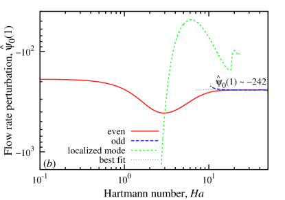
Figure 6: Energy amplitude (a) and the flow rate perturbation (b) at the 2D nonlinear instability threshold for even and odd modes versus the Hartmann number.

Besides the threshold parameters above, the critical 2D travelling wave can also be characterized by its energy amplitude $A_{E}$ and the flow rate perturbation

$$\hat{\psi}_{0}(1)=\int_{0}^{1}(\hat{u}_{0}(z)-\bar{u}_{0}(z))\,dz$$ (32)

which are plotted in figure 6 versus the Hartmann number. At large Ha, the latter is seen to approach $\hat{\psi}_{0}(1)\sim-242,$ which means that the critical flow rate perturbation becomes independent of the magnetic field strength. This is because the flow rate is determined by the product of characteristic length and velocity scales, of which the latter varies inversely with the former. Thus, the Hartmann layer thickness $\delta\sim h/\textit{Ha}$, which defines the characteristic length scale in strong magnetic field, cancels out in the flow rate perturbation. The same arguments also explain the scaling of the energy perturbation (27) inversely with $\textit{Ha},$ which leads to $A_{E}\sim 0.0317\textit{Ha}^{-1/2}$ for the even mode as well as for the odd short-wave mode (see figure 6). The same relation for both instability modes again implies that the perturbations originating in the Hartmann layers at the opposite walls do not affect each other in a sufficiently strong magnetic field (Hagan & Priede, 2013b).

Streamlines of the critical finite-amplitude perturbations of both symmetries are plotted in figure 7 for $\textit{Ha}=10,20.$ Note that the streamlines of the odd mode are mirror-symmetric with respect to the mid-plane $z=0$ whereas those of the even mode posses a central rather than a $z-$reflection symmetry. As discussed in the description of the numerical method, this is because all stream-function harmonics of the odd mode are odd functions of $z$ whereas those of the even mode have alternating $z$ parities. It is interesting to note that the long-wave odd mode at $\textit{Ha}=10$ represents a localized disturbance consisting of a pair of mirror-symmetric vortices. As discussed above, this long-wave equilibrium state disappears at $\textit{Ha}\gtrsim 20.$ The short-wave state, which replaces the former at higher Hartmann numbers, is seen in figure 7 to differ from that of the even mode only by a half-wavelength shift between the top and bottom parts of the channel.

Figure 7: Streamlines of even (a, c) and odd (b, d) critical finite-amplitude perturbations for $\textit{Ha}=10$ (a, b) and $\textit{Ha}=20$ (c, d).

5.2 Linear stability of travelling waves to 2D disturbances

Growth rates of of infinitesimal disturbances of the even travelling-wave mode are plotted in figure 8 for various detuning parameters and $\textit{Ha}=1;5.$ As discussed in Sec. 3.2, the subcritical equilibrium states bifurcating from the base flow are invariably unstable. This is confirmed by the positive growth rate of the fundamental fixed-flow-rate ($Q$) mode , which is seen in figure 8(a) to persist down the lowest Reynolds number $\textit{Re}_{q}$ based on the flow rate. The growth rate of this mode, which is positive and purely real for the unstable lower travelling-wave branch turns negative as the solution passes through the turning point at the critical $\textit{Re}_{q}\approx 3557$ and proceeds to the upper branch. The lower branch can be identified as the one starting from the linear instability threshold at the largest $Re$ while the upper branch as that terminating at $Re_{q}\approx 6000.$ Further this purely negative eigenvalue merges with another similar eigenvalue, which results in two complex-conjugate eigenvalues with negative real part. Note that a purely real growth rate describes disturbances that travel synchronously with the same phase speed as the background wave, whereas the complex growth rate describes asynchronous disturbances which lead to quasi-periodic solutions in the laboratory frame of reference and periodic solutions in the co-moving frame of reference. The change of stability at the lowest value of $\textit{Re}_{q}$ corresponds to a saddle-node bifurcation which occurs at fixed flow rate and gives rise to a stable and unstable branch of travelling-wave states. Owing to the phase invariance of the travelling-wave solution there is always a neutrally stable disturbance corresponding to a small phase shift, i.e. a small shift in $x$ of the original solution.

The growth rate of the fixed-pressure ($P$) mode is plotted in figure 8(a) against the original Reynolds number based on the pressure gradient. This mode is also associated with a saddle-node bifurcation, which in this case occurs at the lowest value $Re.$ As for the $Q$-mode, there is a perturbation with purely real eigenvalue which changes from positive to negative as the travelling-wave solution passes through the turning point at $Re\approx 3962.$ But in contrast to the fixed flow rate, this is not the leading but the second largest eigenvalue. Moreover, conversely to the $Q$-mode, this eigenvalue is negative on the lower branch and positive on the upper branch. At the same time, the leading eigenvalue, which is positive on the lower branch, as for the $Q$-mode, also remains positive after the turning point when the solution passes to the upper branch. Thus, when the flow is driven by fixed pressure gradient, there are two unstable modes with real eigenvalues on the upper travelling-wave branch just after the turning point. At $Re\approx 3972$ these two unstable modes merge forming a pair of modes with complex-conjugate eigenvalues. At $Re\approx 4170$ the real part of the complex-conjugate eigenvalues turns negative and the upper branch of the $P$-mode becomes stable as for the fixed flow rate considered before. These stability characteristic of $Q$- and $P$-modes for $Ha=1$ are not essentially different from those of the non-magnetic Poiseuille flow (Pugh & Saffman, 1988; Soibelman & Meiron, 1991; Casas & Jorba, 2012).

As noted in §3.3, the distinction between fixed-pressure and fixed-flow-rate cases vanishes for detuned modes $(\epsilon\not=0).$ Growth rates of two such modes with $\epsilon=0.25$ and $\epsilon=0.5$ are plotted in figure 8(a). The former is seen to destabilize the lower branch of travelling-wave states only at sufficiently subcritical Reynolds numbers. The latter is a subharmonic disturbance which does the same for the upper branch. Disturbances with $\epsilon=0.75$ and $\epsilon=1$ are found to be stable $(\Re[\tilde{\lambda}]<0)$ and thus not shown here.

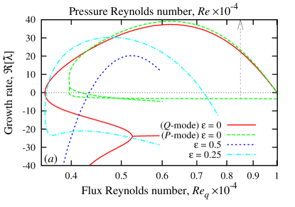
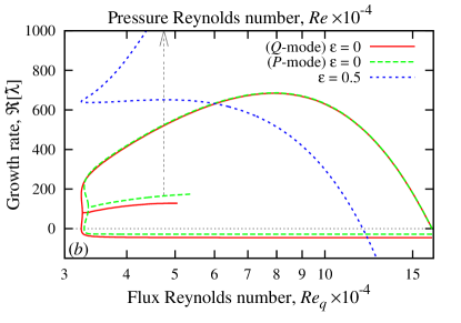
Figure 8: Growth rates of 2D instability modes with various detuning parameters $\epsilon$ versus Reynolds number for $\textit{Ha}=1$ (a) and $\textit{Ha}=5$ (b). All modes except the fixed-pressure $(P)$ mode are plotted against the flux Reynolds number $Re_{q}$ (28). The growth rate of the $P$-mode is plotted against the original Reynolds number based on the mean pressure gradient.

As seen in figure 8(b), the basic features of the $P$-mode at $\textit{Ha}=5$ remain essentially the same as those for $\textit{Ha}=1.$ At the same time, the $Q$-mode changes significantly and closely approaches the $P$-mode. Also, the difference between the pressure and flux Reynolds numbers diminishes with the increase of Hartmann number. As discussed in the previous section, this is due to the localization of perturbations at the walls which results in the reduction of the flow rate perturbation with the increase of Hartman number (see figure 6b). Instability of both solution branches at the turning point implies that additional, possibly quasi-periodic, equilibrium states may exist and also extend towards more subcritical Reynolds numbers as speculated by Barkley (1990) for the non-magnetic case. It is unclear whether such solutions bifurcate from the upper branch as an excessive number of harmonics is required to produce reliable results at higher Reynolds numbers and larger travelling-wave amplitudes.

6 Summary and conclusions

The present study was concerned with 2D nonlinear travelling-wave states in MHD channel flow subject to a transverse magnetic field. Such states are thought to mediate transition to turbulence, which is known to take place in this flow at Reynolds numbers more than two orders of magnitude below the linear stability threshold. Using the Newton-Raphson method, we determined the extension of such 2D nonlinear travelling waves below the linear stability threshold, at which they appear as the result of a subcritical bifurcation. Starting from the non-magnetic plane Poiseuille flow, where these travelling-wave states extend from the linear stability threshold $\textit{Re}{}_{l}=5772$ down to $\textit{Re}{}_{n}=2939,$ and gradually increasing the magnetic field, we found that in a sufficiently strong magnetic field $(Ha\gtrsim 10)$ such states extend down to $\textit{Re}{}_{n}\sim 6.50\times 10^{3}\textit{Ha.}$ Although this Reynolds number is almost an order of magnitude lower than the linear stability threshold of the Hartmann flow, it is still morethan an order of magnitude greater than that at which turbulence is observed in this type of flow.

Besides the solution which evolves from plane Poiseuille flow as the magnetic field is increased, we found another inherently magnetohydrodynamic solution which bifurcates subcritically from the Hartmann flow at $Ha\approx 6.5.$ The two solutions differ by their $z$-symmetries: the harmonics of the transverse velocity are odd functions of $z$ for the latter and they have alternating parities starting with even one for the former. The odd-symmetry solution was found to have two branches. The first branch, which exists in a limited range of the magnetic field strength with $2.8\lesssim Ha\lesssim 20,$ has a relatively long wavelength and consists of a pair of intense localized vortices. The second branch, which emerges at $Ha\approx 10$ with a much shorter wavelength, has very similar characteristics to the original hydrodynamic branch, and becomes practically indistinguishable from the latter when $Ha\gtrsim 20.$ We also showed that the lower-amplitude 2D travelling waves, as in the non-magnetic case, are invariably unstable with respect to 2D infinitesimal superharmonic disturbances down to the limiting value of the Reynolds number based on the flow rate.

Subcritical 2D travelling waves in the Hartmann flow are also likely to be unstable to more general three-dimensional disturbances similar to those considered by Orszag & Patera (1983) in the non-magnetic case. Three-dimensional equilibrium states bifurcating either from 2D travelling waves (Ehrenstein & Koch, 1991) or infinity (Waleffe, 2001), as in plane Poiseuille flow, may extend to significantly lower Reynolds numbers and, thus, provide a more adequate threshold for the onset of turbulence in the Hartmann flow. Such a possibility is supported by the interaction of only two mirror-symmetric oblique waves with the resulting 2D second harmonic considered by Zinovév & Shtern (1987), who found, for the Hartmann layer, $R_{n}\approx 4670.$ As for the 2D waves considered in this study, it is likely that a more adequate three-dimensional model including a sufficient number of higher harmonics could result in a substantially lower $R_{n}.$